Climate Stress Testing - newyorkfed.org

Climate Stress Testing

Hyeyoon Jung | Robert Engle | Richard Berner

NO. 977

SEPTEM BER 2021

Climate Stress Testing

Hyeyoon Jung, Robert Engle, and Richard Berner

Federal Reserve Bank of New York Staff Reports, no. 977

September 2021

JEL classification: Q54, C53, G20

Abstract

Climate change could impose systemic risks upon the financial sector, either via disruptions in economic

activity resulting from the physical impacts of climate change or changes in policies as the economy

transitions to a less carbon-intensive environment. We develop a stress testing procedure to test the

resilience of financial institutions to climate-related risks. Specifically, we introduce a measure called

CRISK, systemic climate risk, which is the expected capital shortfall of a financial institution in a climate

stress scenario. We use the measure to study the climate-related risk exposure of large global banks in the

collapse of fossil-fuel prices in 2020.

Key words: climate risk, financial stability, stress testing

_________________

Jung: Federal Reserve Bank of New York (email: [email protected]). Engle, Berner: Stern

School of Business, New York University (email: [email protected], [email protected].). The

authors thank German Gutierrez, Quirin Fleckenstein, Sebastian Hillenbrand, and participants at the

Volatility and Risk Institute Conference, EBA EAIA Seminar, and Green Swan Conference for their

helpful comments and suggestions. They also thank Georgij Alekseev for excellent research assistance.

This paper presents preliminary findings and is being distributed to economists and other interested

readers solely to stimulate discussion and elicit comments. The views expressed in this paper are those of

the author(s) and do not necessarily reflect the position of the Federal Reserve Bank of New York or the

Federal Reserve System.

To view the authors’ disclosure statements, visit

https://www.newyorkfed.org/research/staff_reports/sr977.html.

1 Introduction

Understanding the impact of climate change on financial systems is an important question

for researchers, central banks, and financial regulators across the world. Krueger et al.

(2020) find that institutional investors believe climate risks have financial implications for

their portfolio firms and that these risks have already begun to materialize. Many central

banks have recently started including climate stress scenarios in their own stress testing

frameworks.1 The Network of Central Banks and Supervisors for Greening the Financial

System (NGFS), which consists of 89 member countries as of March 2021, analyzes the

impact of climate change on macroeconomic and financial stability.2

How does climate change impose systemic risks on the financial sector? Two main chan-

nels are: first, through disruptions of economic activity resulting from the physical impacts

of climate change; second, through the changes in policies as economies transition to a less

carbon-intensive environment. The former are referred to as physical risks and the latter are

referred to as transition risks.3 Physical risks can affect financial institutions through their

exposures to firms and households that experience extreme weather shocks. On the other

hand, transition risks can affect financial institutions through their exposures to firms with

business models not aligned with a low-carbon economy. Fossil fuel firms are a prominent

example: banks that provide financing to fossil fuel firms are expected to suffer when the

default risk of their loan portfolios increases, as economies transition into a lower-carbon

environment. If banks systemically suffer substantial losses following an abrupt rise in the

physical risks or transition risks, climate change poses a considerable risk to the financial

1For example, the central banks and the regulators of Australia, Canada, England, France, and theNetherlands have already begun performing climate stress tests, or have announced their intention to conductsuch tests.

2See https://www.ngfs.net/en for further details on NGFS.3NGFS defines physical risks as financial risks that can be categorized as either acute—if they arise from

climate and weather-related events and acute destruction of the environment—or chronic—if they arise fromprogressive shifts in climate and weather patterns or from the gradual loss of ecosystem services. NGFSdefines transition risks as financial risks which can result from the process of adjustment towards a lower-carbon and more circular economy, prompted, for example, by changes in climate and environmental policy,technology, or market sentiment (NGFS (2020)).

1

https://www.ngfs.net/en

system.

How much systemic risk does climate change impose on the financial system? This

question is at the heart of understanding the impact of climate change on financial systems.

We contribute to answering the question by developing a climate stress testing methodology

to test the resilience of financial institutions to climate-related risks. Specifically, we develop

a measure called CRISK, which is the expected capital shortfall of a financial institution in

a climate stress scenario. The stress testing procedure involves three steps. The first step

is to measure the climate risk factor. While there are many ways to measure the climate

risk factor, we use stranded asset portfolio return as a proxy measure for transition risk.

The second step is to estimate a time-varying climate beta of financial institutions using

the Dynamic Conditional Beta (DCB) model. The third step is to compute CRISK, which

is a function of a given financial firm’s size, leverage, and expected equity loss conditional

on climate stress. This step is based on the same methodology as SRISK of Acharya et

al. (2011), Acharya et al. (2012), and Brownlees and Engle (2017), with the climate factor

added as the second factor.

We apply the methodology to measure the climate risk of 27 large global banks, whose

aggregate oil and gas loan market share exceeds 80%. The stress scenario that we consider

is a 50% drop in the return on stranded asset portfolio over six months. This corresponds to

the first percentile of historical return on stranded asset portfolio. We find that, first, climate

beta varies over time, highlighting the importance of dynamic estimation. Second, climate

betas of banks move together over time, and there was a common spike in climate betas as

well as in CRISKs when energy prices collapsed in 2020. The measured CRISKs for some

of the banks were economically substantial. For instance, Citigroup’s CRISK increased by

73 billion US dollars during the year 2020. In other words, the expected amount of capital

that Citigroup would need to raise under the climate stress scenario to restore a prudential

capital ratio4 increased by 73 billion US dollars in 2020. In a decomposition analysis, we find

4We set prudential capital ratio as 8%.

2

that the increase in CRISK during 2020 is primarily due to decreases in the equity values

of banks, as opposed to decreases in debt values or increases in climate betas. Third, we

find evidence that banks with higher loan exposure to the oil and gas industry tend to have

higher climate betas, corroborating the economic validity of our climate beta estimates.

Related Literature

This paper contributes to several strands of literature. First, it adds to the growing body

of literature on climate finance. Giglio et al. (2020) provide a review on the literature

regarding the pricing of climate risks across different asset classes. Studies including Bolton

and Kacperczyk (2020), Engle et al. (2020), and Ilhan et al. (2020) suggest that climate

risks are priced in the equity market. A few papers also have examined the effects of climate

change on banks’ loan pricing. Chava (2014) finds that banks charge a significantly higher

interest rate on the loans provided to firms with environmental issues. Ginglinger and

Quentin (2019) find consistent evidence that greater climate risk leads to lower leverage

after the Paris Agreement, partly because lenders increase the spreads when lending to firms

with the greatest climate risk. We add to the literature by quantifying the climate-related

risk exposure of financial institutions. Despite the evidence that banks do price climate

risks, our CRISK measures suggest that climate change could lead to a substantial increase

in systemic risks when transition risks rise sharply.

This paper also contributes to the literature on stress testing and systemic risk measure-

ment. In the context of climate-related stress testing, Reinders et al. (2020) use Merton’s

contingent claims model to assess the impact of a carbon tax shock on the value of corpo-

rate debt and residential mortgages in the Dutch banking sector. Compared to other stress

testing methodologies, CRISK methodology inherits the benefits of the SRISK methodology

of Acharya et al. (2011), Acharya et al. (2012), and Brownlees and Engle (2017). First,

CRISK does not require any proprietary information and can be readily computed using

publicly available data on the balance sheet and market information of each financial in-

3

stitution and the return on stranded asset portfolio. Moreover, it can be estimated on a

high-frequency basis. Therefore, it is very easy to estimate and promptly reflects current

market conditions. It is thus a useful monitor that enables regulators to respond in a timely

manner in the case intervention is necessary. Second, CRISK measures the expected capital

shortfall conditional on aggregate stress. That is, we are not measuring how much capital a

bank would need when the bank is under stress in isolation. Third, firm-level CRISK can be

aggregated to country-level CRISK, which provides early warning signals of macroeconomic

distress due to climate change. Fourth, by applying a consistent methodology to different

firms in different countries, the CRISK measure allows comparison across firms and across

countries. Lastly, implementing the CRISK measure offers value incremental to other stress

testing methodologies that are already in place. Previous studies including Acharya et al.

(2014) and Brownlees and Engle (2017) show that regulatory capital shortfalls measured

relative to total assets give similar rankings to SRISK. However, rankings are different when

the regulatory capital shortfalls are measured relative to risk-weighted assets, and they are

also different from those observed in the European stress tests.

Outline of the Paper

The remainder of the paper proceeds as follows: Section 2 describes the data. Section 3

develops our empirical methodology and reports the stress testing results. Section 4 analyzes

the CRISKs of large global banks during 2020. Section 5 tests the economic validity of our

estimates. Section 6 discusses future directions for research, and section 7 concludes.

2 Data

We estimate climate betas and CRISKs of large global banks in the U.S., the U.K., Canada,

Japan, and France for the sample period from 2000 to 2020. We focus on the large global

banks as they hold more than 80% of syndicated loans made to oil and gas industry. The

4

list of top 50 global banks by oil and gas loan exposure is presented in Table 25 in the

Appendix. We use the return on an S&P 500 ETF for the market return. The stock return

and accounting data of banks are from Datastream, and syndicated loan data is from LPC

DealScan and Bloomberg League Table. We use the DealScan-Compustat link from Schwert

(2018).

3 Methodology and Empirical Results

The climate stress testing procedure involves three steps. The first step is to measure the

climate risk factor by using stranded asset portfolio return as a proxy measure for transition

risk. The second step is to estimate the time-varying climate betas of financial institutions

using the DCB model. The third step is to compute CRISK, which is a function of a given

firm’s size, leverage, and expected equity loss conditional on climate stress. This step extends

the SRISK methodology of Acharya et al. (2011), Acharya et al. (2012), and Brownlees and

Engle (2017) by adding the climate factor as the second factor.

3.1 Climate Factor Measurement

There are several ways to measure the climate risk factor, including the climate news index

constructed by Engle et al. (2020). We use Litterman’s ”stranded asset” portfolio return as

a measure of transition risks.5 The stranded asset portfolio consists of a long position in the

stranded asset index comprised of 30% in Energy Select Sector SPDR ETF (XLE) and 70%

in VanEck Vectors Coal ETF (KOL), and a short position in SPDR S&P 500 ETF Trust

(SPY ). We directly use the return on stranded asset portfolio as the climate factor:

CF Str = 0.3XLE + 0.7KOL− SPY

5This acts as a proxy for the World Wildlife Fund stranded assets total return swap. See http://www.

intentionalendowments.org/selling_stranded_assets_profit_protection_and_prosperity for fur-ther details.

5

http://www.intentionalendowments.org/selling_stranded_assets_profit_protection_and_prosperity

http://www.intentionalendowments.org/selling_stranded_assets_profit_protection_and_prosperity

because it can be easily computed on a daily basis, and the portfolio is expected to under-

perform as economies transition to a lower-carbon economy. A short position in the stranded

asset portfolio is a bet on the underperformance of coal and other fossil fuel firms; there-

fore, a lower value of CF Str indicates underperformance of fossil fuel firms and hence higher

transition risk. Since the VanEck Vectors Coal ETF started in 2008 and was liquidated in

2020, the climate factor is computed as:

CF Str = XLE − SPY

for the period outside of 2008–2020. Figure 1 shows that the cumulative return on the

stranded asset portfolio has been falling since 2011.

Figure 1: Stranded Asset Portfolio Cumulative Return

0

1

2

3

4

Cum

ulat

ive

Per

form

ance

01jan2000 01jan2005 01jan2010 01jan2015 01jan2020Date

XLE − SPY 0.3 XLE + 0.7 KOL − SPY

3.2 Climate Beta Estimation

We use the DCB model to estimate the time-varying climate betas. The GARCH-DCC

model of Engle (2002), Engle (2009), and Engle (2016) allows volatility and correlation to

6

be time-varying. Following the standard factor model approach, we model bank i’s stock

return as:

rit = βMktit MKTt + βClimate

it CFt + εit,

where rit is the stock return of bank i, MKT is the market return, and CF is the climate

factor, measured as the return on the stranded asset portfolio. The market beta and climate

beta, in this regression, measure the sensitivity of bank i to market risk and to transition-

related climate risk, respectively. One would expect that banks with large amounts of loans

in the fossil fuel industry will be more sensitive to climate risk on average and will have a

positive climate beta. However, in the case that a bank holds a large amount of loans in the

renewable energy sector, the bank’s climate beta could be negative.

For stock markets with a closing time different from that of the New York market, we take

asynchronous trading into consideration by including the lags of the independent variables:

rit = βMkt1it MKTt + βMkt

2it MKTt−1 + βClimate1it CFt + βClimate

2it CFt−1 + εit

Assuming that returns are serially independent, we estimate the following two specifications

separately and sum the coefficients.

rit = βMkt1it MKTt + βClimate

1it CFt + εit

rit = βMkt2it MKTt−1 + βClimate

2it CFt−1 + εit

The sum, βMkt1it + βMkt

2it , is the estimate of market beta and the sum, βClimate1it + βClimate

2it , is

the estimate of climate beta.

We present the estimated climate betas of large global banks in the U.S., U.K., Canada,

Japan, and France in Figures 2–6. For illustration, we plot the six-month moving averages

of the estimates. We report the non-smoothed climate beta estimates and market beta

estimates in the Appendix.

7

Figure 2: Climate Beta of U.S. Banks

2002 2004 2006 2008 2010 2012 2014 2016 2018 2020-0.6

-0.4

-0.2

0

0.2

0.4

0.6

0.8C

limat

e B

eta

Climate Beta

BAC:USBK:USC:USCOF:USGS:US

JPM:USMS:USPNC:USUSB:USWFC:US

Figure 3: Climate Beta of U.K. Banks

2005 2010 2015 2020-1

-0.8

-0.6

-0.4

-0.2

0

0.2

0.4

0.6

0.8

1

Clim

ate

Bet

a

Climate Beta

BARC:LNHSBA:LNLLOY:LNNWG:LNSTAN:LN

8

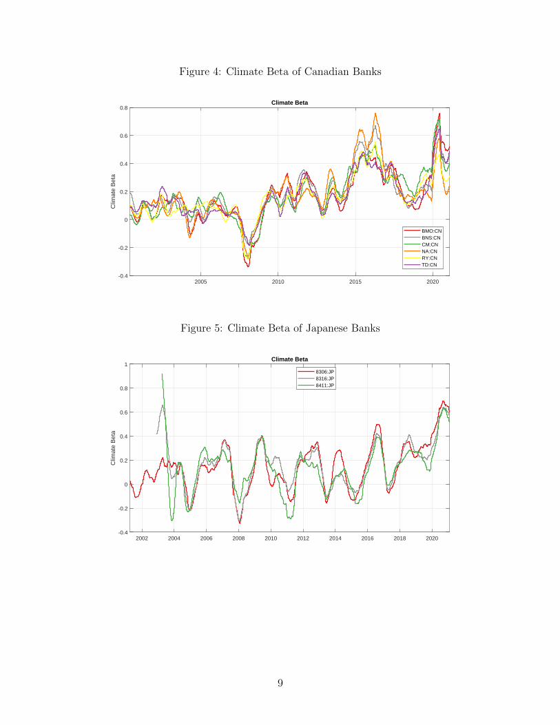
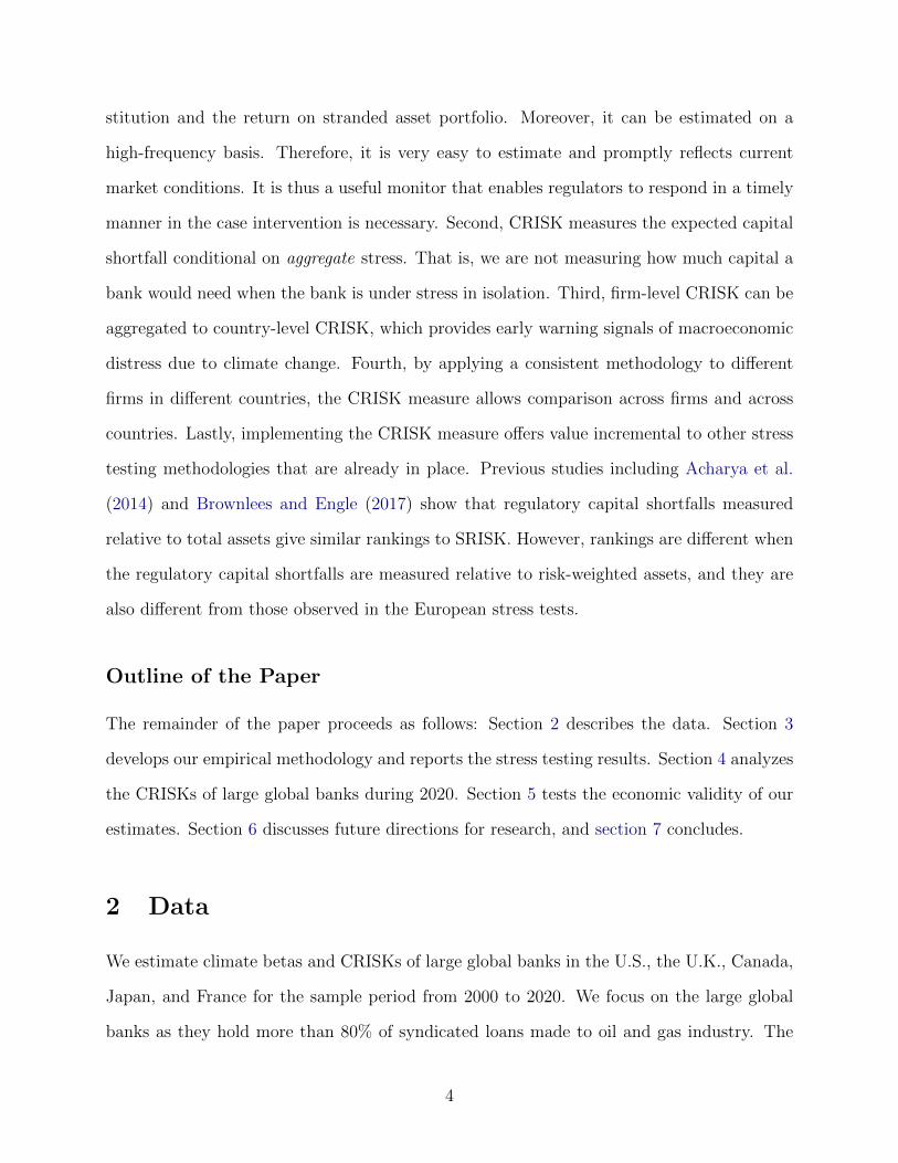
Figure 4: Climate Beta of Canadian Banks

2005 2010 2015 2020-0.4

-0.2

0

0.2

0.4

0.6

0.8C

limat

e B

eta

Climate Beta

BMO:CNBNS:CNCM:CNNA:CNRY:CNTD:CN

Figure 5: Climate Beta of Japanese Banks

2002 2004 2006 2008 2010 2012 2014 2016 2018 2020-0.4

-0.2

0

0.2

0.4

0.6

0.8

1

Clim

ate

Bet

a

Climate Beta

8306:JP8316:JP8411:JP

9

Figure 6: Climate Beta of French Banks

2005 2010 2015 2020-0.6

-0.4

-0.2

0

0.2

0.4

0.6

0.8

1

1.2C

limat

e B

eta

Climate Beta

ACA:FPBNP:FPGLE:FP

Based on the estimation results, we summarize the main findings as follows. First, it is

worth noting that climate beta varies over time, and therefore it is important to estimate

the betas dynamically. Second, we observe a common spike in the year 2020 as banks’

exposures to the transition risk rose substantially due to a collapse in energy prices. Third,

the average level of climate beta is different across countries, and this could be due to

differences in country-specific climate-related regulations, or differences in climate-conscious

investing patterns across countries. In the U.S., the climate beta estimates range from −0.4

to 0.7, and were often not significantly different from zero before 2015. In terms of magnitude,

a climate beta of 0.5 means that a 1% fall in the stranded asset portfolio return is associated

with a 0.5% fall in the bank’s stock return. The climate beta estimates’ proximity to zero

could be related to the non-linearity in climate beta as a function of the return on stranded

asset portfolio. That is, we expect that the values of bank stocks are relatively insensitive to

fluctuations in the stock prices of oil and gas firms as long as they are sufficiently far from

default. On the other hand, the estimates for UK banks were higher on average.

10

3.3 CRISK Estimation

Following SRISK methodology in Acharya et al. (2011), Acharya et al. (2012), Brownlees

and Engle (2017), CRISK for each financial institution is computed as:

CRISKit = k ·DEBTit − (1 − k) · EQUITYit · (1 − LRMESit) (1)

= k ·DEBTit − (1 − k) · EQUITYit · exp(βClimateit log(1 − θ)

)(2)

where βClimateit is the climate beta of bank i, DEBT is book value of debt (book value

of assets less book value of equity), and EQUITY is market capitalization. LRMES is

long-run marginal expected shortfall, the expected stock return conditional on the systemic

climate event. We set the prudential capital fraction k to 8% and the climate stress level

θ to 50%. This corresponds to the first percentile of six-month return (fractional) on the

stranded assets. The summary statistics are included in the Appendix. Figures 7–11 present

the estimated CRISKs of large global banks in the U.S., U.K., Canada, Japan, and France.

The estimated CRISKs are often negative until 2019. As CRISK is the expected capital

shortfall, a negative CRISK indicates that the bank holds a capital surplus. This is likely

related to the non-linear relationship between climate beta and the performance of fossil-fuel

firms. A bank will not have a capital shortfall if its climate beta is small and therefore has a

negative CRISK. In contrast, the CRISKs increased substantially across countries in 2020.

Since CRISK is a function of climate beta, as well as a function of the size and leverage of a

bank, the ranking of CRISKs can differ from that of the climate beta estimates. For instance,

while the climate beta estimates of the U.S. banks were relatively low, their CRISKs were

substantial, as high as 95 billion USD for Citibank in June 2020. To put this into context,

Citibank’s SRISK, the expected capital shortage in a potential future financial crisis, was

125 billion USD in June 2020.6 In contrast, CRISKs of Canadian banks in June 2020 range

from 6 billion to 33 billion USD, despite their high climate betas.

6NYU’s V-lab (https://vlab.stern.nyu.edu/) provides systemic risk analysis.

11

https://vlab.stern.nyu.edu/

Figure 7: CRISK of U.S. Banks

2002 2004 2006 2008 2010 2012 2014 2016 2018 2020-200

-150

-100

-50

0

50

100

150C

RIS

K (

$bio

)

CRISK (US Banks)



Figure 8: CRISK of U.K. Banks

2005 2010 2015 2020-100

-50

0

50

100

150

200

250

300

CR

ISK

($b

io)

CRISK (UK Banks)


12

Figure 9: CRISK Beta of Canadian Banks

2005 2010 2015 2020-30

-20

-10

0

10

20

30

40C

RIS

K (

$bio

)

CRISK (CN)


Figure 10: CRISK Beta of Japanese Banks

2002 2004 2006 2008 2010 2012 2014 2016 2018 2020-50

0

50

100

150

200

CR

ISK

($b

io)

CRISK (JP)

8306:JP8316:JP8411:JP

13

Figure 11: CRISK of French Banks

2005 2010 2015 20200

50

100

150

200

250C

RIS

K (

$bio

)

CRISK (FP)

ACA:FPBNP:FPGLE:FP

4 Discussion

Given that CRISKs increased substantially in 2020, we focus on the first half of 2020 and

analyze CRISKs in relation to banks’ loan exposure to the oil and gas industry. In this

section, we first provide suggestive evidence that our CRISK measure during 2020 roughly

aligns with the size of currently active loans made to the U.S. firms in the oil and gas industry.

Then, we decompose the CRISK estimates into the components due to debt, equity, and risk,

respectively. We find that a decline in the equity component contributes the most to the

overall increase in CRISKs.

U.S. Banks

Figure 12 overlays the CRISK measures of the U.S. banks, and Table 1 tabulates the banks’

exposure to the oil and gas industry. LenderAmt is the sum of all active loans from the bank

to U.S. firms in the oil and gas industry as of April 2020.7

7We appreciate Sascha Steffen for sharing this measure.

14

Figure 12: Climate SRISK, US Large Banks, SPY

Jan Apr Jul Oct Jan2020

0

20

40

60

80

100

120

140

CR

ISK

($b

io)

CRISK in 2020 (US Banks)



Table 1: US Bank Exposure to the Oil & Gas Industry

No Name Ticker LenderAmt1 Wells Fargo WFC 46,9392 JP Morgan JPM 38,7923 BofA BAC 29,7204 Citi C 28,0725 US Bancorp USB 12,0916 PNC Bank PNC 11,8187 Goldman Sachs GS 11,5978 Morgan Stanley MS 10,0249 Capital One Financial Corp COF 9,62110 Bank of New York Mellon BK 1,289

To better understand what drives variation in CRISK, we decompose climate SRISK into

three components based on Equation 1:

dCRISK = k · ∆DEBT︸︷︷︸dDEBT

−(1 − k)(1 − LRMES) · ∆EQUITY︸︷︷︸dEQUITY

+ (1 − k) · EQUITY · ∆LRMES︸︷︷︸dRISK

,

15

where LRMES is the long-run marginal expected shortfall, EQUITY is market capitaliza-

tion, and DEBT is book value of debt. The first component, dDEBT = k ·∆DEBT is the

contribution of the firm’s debt to CRISK. CRISK increases as the firm takes on more debt.

The second component, dEQUITY = −(1 − k)(1 − LRMESt) · ∆EQUITY is the effect of

the firm’s equity position on CRISK. CRISK increases as the firm’s market capitalization

deteriorates. The third component, dRISK = (1 − k) · EQUITYt−1 · ∆LRMES is the

contribution of increase in volatility or correlation to CRISK.

Table 2: CRISK Decomposition

CRISK(t) is the bank’s CRISK at the end of 2020, and CRISK(t − 1) is CRISK at thebeginning of year 2020. dCRISK= CRISK(t)-CRISK(t− 1) is the change in CRISK during2020. dDEBT is the contribution of the firm’s debt to CRISK. dEQUITY is the contributionof the firm’s equity position on CRISK. dRISK is the contribution of increase in volatilityor correlation to CRISK. All amounts are in billions USD.

Bank CRISK(t-1) CRISK(t) dCRISK dDEBT dEQUITY dRISKBAC:US -60.5598 15.0086 75.5684 24.6334 54.9075 -4.4293BK:US -8.6035 4.6776 13.2811 4.1082 9.8573 -0.89512C:US 5.1582 81.9642 76.8061 17.4887 42.0878 15.939COF:US -11.5581 -3.3809 8.1772 3.2452 6.1094 -0.61547GS:US 9.0332 12.748 3.7147 9.8983 -1.0523 -5.3841JPM:US -148.5589 -48.5246 100.0343 38.4204 73.4622 -14.1743MS:US 2.0322 -21.5796 -23.6117 3.65 -23.7485 -3.9269PNC:US -28.33 -12.5543 15.7758 3.8029 13.6699 -1.4535USB:US -39.8808 -10.8763 29.0045 4.131 23.16 1.3047WFC:US -48.1845 62.8932 111.0777 -0.84144 105.7064 5.3232

Table 2 decomposes the change in CRISK during the year 2020 into the three components.

The decomposition suggests that the decline in equity contributes the most to the increase

in CRISK. Put differently, banks were already stressed without the climate stress scenario.

Nevertheless, the difference between CRISK and non-stressed CRISK is sizable for the largest

banks including Bank of America, Citi, and JP Morgan. Figure 13 plots the CRISK and

non-stressed CRISK, which is the CRISK when the climate stress level θ is set to be zero.

16

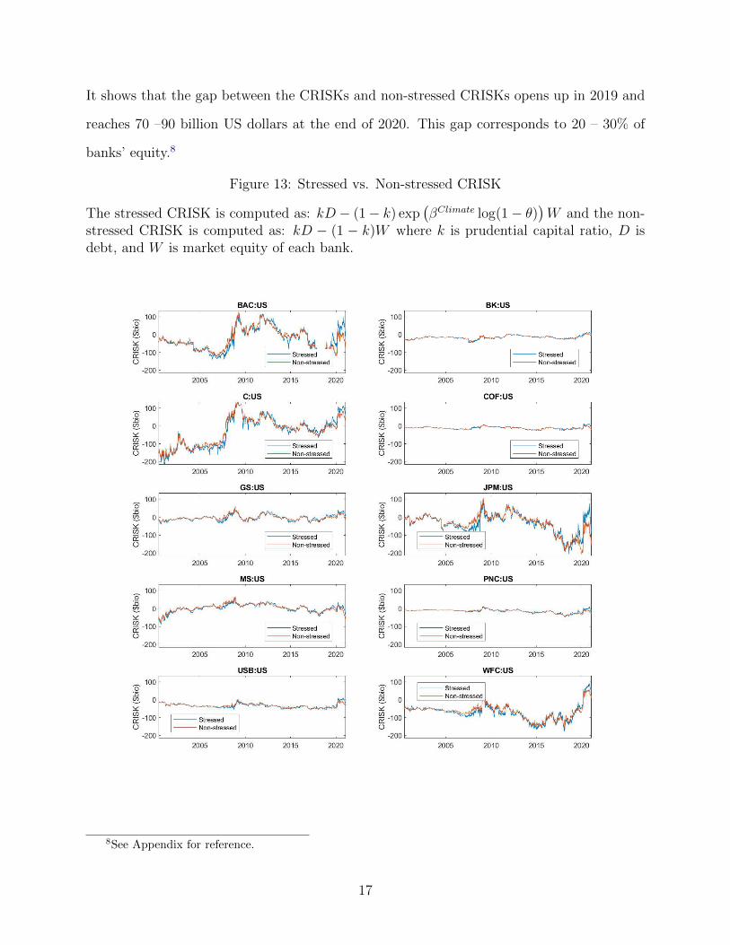
It shows that the gap between the CRISKs and non-stressed CRISKs opens up in 2019 and

reaches 70 –90 billion US dollars at the end of 2020. This gap corresponds to 20 – 30% of

banks’ equity.8

Figure 13: Stressed vs. Non-stressed CRISK

The stressed CRISK is computed as: kD − (1 − k) exp(βClimate log(1 − θ)

)W and the non-

stressed CRISK is computed as: kD − (1 − k)W where k is prudential capital ratio, D isdebt, and W is market equity of each bank.

8See Appendix for reference.

17

U.K. Banks

We document similar findings for the U.K. banks. Figure 14, Table 3 and Table 4 present

the results for the U.K. banks.

Figure 14: Climate SRISK, US Large Banks, SPY

Jan 2020 Apr 2020 Jul 2020 Oct 2020 Jan 2021 Apr 202120

40

60

80

100

120

140

160

180

200

CR

ISK

($b

io)

CRISK in 2020 (UK Banks)


Table 3: UK Bank Exposure to the Oil & Gas Industry

No Name Ticker LenderAmt1 Barclays BARC 19,8932 HSBC Banking Group HSBC 7,5463 Standard Chartered Bank STAN 3,9454 Natwest NWG 1,3615 Lloyds Banking Group LLOY 869

18

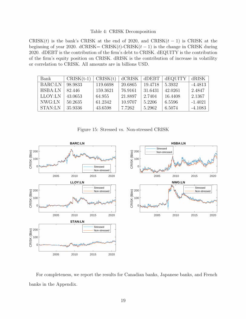
Table 4: CRISK Decomposition

CRISK(t) is the bank’s CRISK at the end of 2020, and CRISK(t − 1) is CRISK at thebeginning of year 2020. dCRISK= CRISK(t)-CRISK(t− 1) is the change in CRISK during2020. dDEBT is the contribution of the firm’s debt to CRISK. dEQUITY is the contributionof the firm’s equity position on CRISK. dRISK is the contribution of increase in volatilityor correlation to CRISK. All amounts are in billions USD.

Bank CRISK(t-1) CRISK(t) dCRISK dDEBT dEQUITY dRISKBARC:LN 98.9833 119.6698 20.6865 19.4718 5.3932 -4.4813HSBA:LN 82.446 159.3621 76.9161 31.6431 42.0261 2.4847LLOY:LN 43.0653 64.955 21.8897 2.7404 16.4408 2.1367NWG:LN 50.2635 61.2342 10.9707 5.2206 6.5596 -1.4021STAN:LN 35.9336 43.6598 7.7262 5.2962 6.5074 -4.1083

Figure 15: Stressed vs. Non-stressed CRISK

2005 2010 2015 2020

0

100

200

CR

ISK

($b

io)

BARC:LN

StressedNon-stressed

2005 2010 2015 2020

0

100

200

CR

ISK

($b

io)

HSBA:LN


2005 2010 2015 2020

0

100

200

CR

ISK

($b

io)

LLOY:LN


2005 2010 2015 2020

0

100

200

CR

ISK

($b

io)

NWG:LN


2005 2010 2015 2020

0

100

200

CR

ISK

($b

io)

STAN:LN


For completeness, we report the results for Canadian banks, Japanese banks, and French

banks in the Appendix.

19

5 Robustness Check

As a robustness check, we first confirm the positive relationship between banks’ climate beta

and their exposure to oil and gas loans. Figure 16 shows that banks with a higher amount

of active syndicated loans had higher climate betas in the second quarter of 2020.

Figure 16: US banks’ climate beta and exposure to oil and gas loans

US banks’ average climate beta and log of active syndicated loans to oil and gas sector inthe second quarter of 2020.9

JPM

C

USB

BAC

WFCPNC

MS

COF

GS.2

.3

.4

.5

.6

Clim

ate

Bet

a

8.5 9 9.5 10 10.5Active GO Loans

To formally test the hypothesis, we use the following specification:

∆βClimateit = a+ b ·GOLoansi,t−1 + εit

where βClimateit is bank i’s time-averaged dynamically-estimated daily climate beta during

quarter t. GOLoansit is bank i’s new syndicated loans to the US oil and gas industry (in

log) in quarter t.10 Standard errors are clustered by banks. Table 26 in Appendix shows

10The syndicated facility amount is equally allocated among the lead banks, and institutional term loans

20

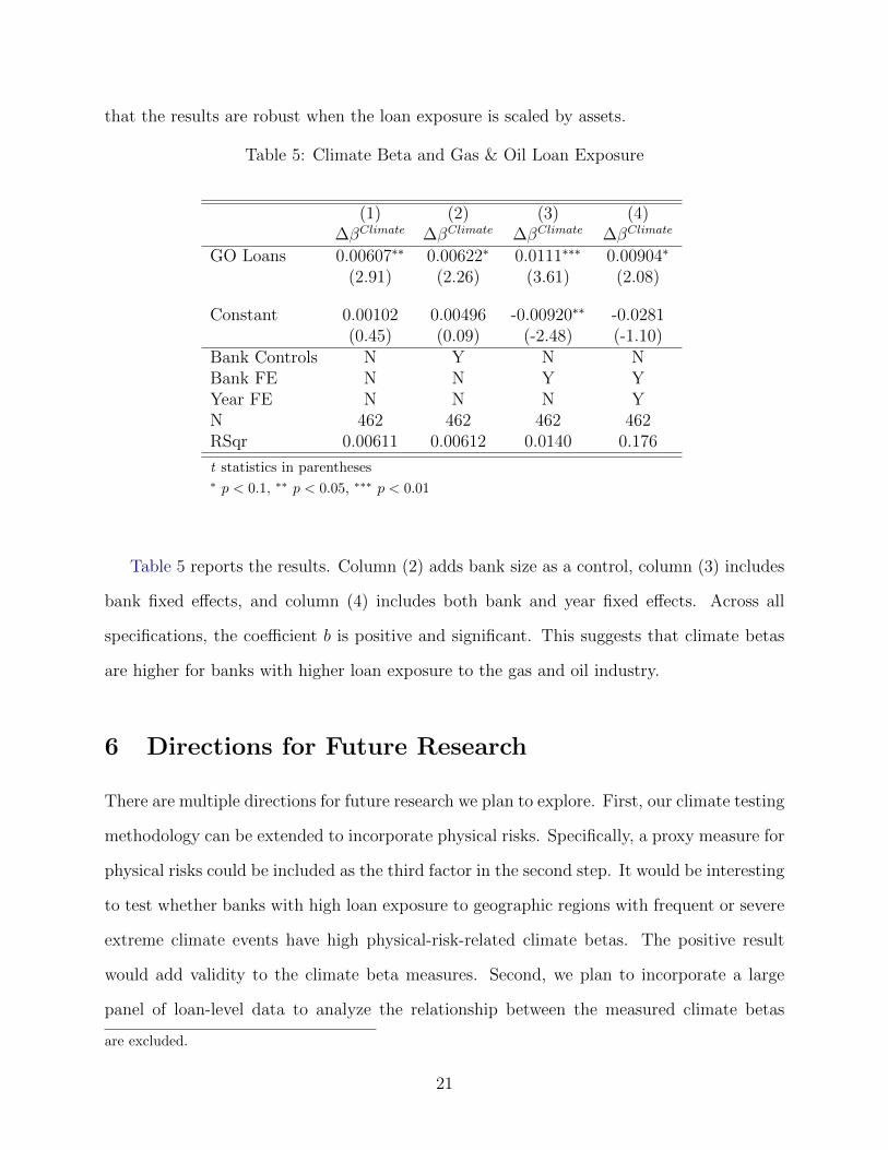
that the results are robust when the loan exposure is scaled by assets.

Table 5: Climate Beta and Gas & Oil Loan Exposure

(1) (2) (3) (4)∆βClimate ∆βClimate ∆βClimate ∆βClimate

GO Loans 0.00607∗∗ 0.00622∗ 0.0111∗∗∗ 0.00904∗

(2.91) (2.26) (3.61) (2.08)

Constant 0.00102 0.00496 -0.00920∗∗ -0.0281(0.45) (0.09) (-2.48) (-1.10)

Bank Controls N Y N NBank FE N N Y YYear FE N N N YN 462 462 462 462RSqr 0.00611 0.00612 0.0140 0.176

t statistics in parentheses∗ p < 0.1, ∗∗ p < 0.05, ∗∗∗ p < 0.01

Table 5 reports the results. Column (2) adds bank size as a control, column (3) includes

bank fixed effects, and column (4) includes both bank and year fixed effects. Across all

specifications, the coefficient b is positive and significant. This suggests that climate betas

are higher for banks with higher loan exposure to the gas and oil industry.

6 Directions for Future Research

There are multiple directions for future research we plan to explore. First, our climate testing

methodology can be extended to incorporate physical risks. Specifically, a proxy measure for

physical risks could be included as the third factor in the second step. It would be interesting

to test whether banks with high loan exposure to geographic regions with frequent or severe

extreme climate events have high physical-risk-related climate betas. The positive result

would add validity to the climate beta measures. Second, we plan to incorporate a large

panel of loan-level data to analyze the relationship between the measured climate betas

are excluded.

21

and the banks’ loan portfolio composition. Third, we could perform the stress test using a

different measure of climate factor. For instance, using records of historical changes in the

climate-related policies across countries would be one useful way to analyze transition risks.

Fourth, we can aggregate bank-level CRISK to country-level CRISK, which can be used as

a warning signal of macroeconomic distress due to climate risks.

7 Conclusion

Climate change could impose systemic risk to the financial sector through either disruptions

of economic activity resulting from the physical impacts of climate change or changes in

policies as the economy transitions to a less carbon-intensive environment. We develop a

stress testing procedure to test the resilience of financial institutions to climate-related risks.

The procedure involves three steps. The first step is to measure the climate risk factor.

We propose using stranded asset portfolio returns as a proxy measure of transition risks.

The second step is to estimate the time-varying climate betas of financial institutions. We

estimate dynamically by using the DCB model to incorporate time-varying volatility and

correlation. The third step is to compute the CRISKs, the capital shortfall of financial

institutions in a climate stress scenario. This step is based on the same methodology as

SRISK, but the climate factor is added as the second factor. We use this procedure to study

the climate risks of large global banks in the U.S., U.K., Canada, Japan, and France in

the collapse in fossil fuel prices in 2020. We document a substantial rise in climate betas

and CRISKs across banks during 2020 when energy prices collapsed. Further, we provide

evidence that banks with a higher exposure to the fossil fuel industry tend to have higher

climate betas, adding validity to our CRISK measure.

22

References

Acharya, Viral, Robert Engle, and Diane Pierret, “Testing macroprudential stresstests: The risk of regulatory risk weights,” Journal of Monetary Economics, 2014, 65, 36– 53.

Acharya, Viral V., Christian T. Brownlees, Farhang Farazmand, and MatthewRichardson, “Measuring Systemic Risk,” Regulating Wall Street: The Dodd-Frank Actand the New Architecture of Global Finance, chapter 4, 2011.

, Robert F. Engle, and Matthew Richardson, “Capital Shortfall: A New Approachto Ranking and Regulating Systemic Risks,” American Economic Review: Papers andProceedings, 2012.

Bolton, Patrick and Marcin T. Kacperczyk, “Do Investors Care about Carbon Risk?,”Journal of Financial Economics, 2020.

Brownlees, Christian T. and Robert F. Engle, “SRISK: A Conditional Capital Short-fall Index for Systemic Risk Measurement,” Review of Financial Studies, 2017.

Chava, Sudheer, “Environmental Externalities and Cost of Capital,” Management Science,2014, 60 (9), 2223–2247.

Engle, Robert F., “Dynamic conditional correlation: A simple class of multivariate gen-eralized autoregressive conditional heteroscedasticity models,” Journal of Business andEconomic Statistics, 2002.

, “Anticipating correlations: A new paradigm for risk management,” Princeton, NJ:Princeton University Press, 2009.

, “Dynamic Conditional Beta,” Journal of Financial Econometrics, 2016.

Engle, Robert F, Stefano Giglio, Bryan Kelly, Heebum Lee, and JohannesStroebel, “Hedging Climate Change News,” The Review of Financial Studies, 02 2020,33 (3), 1184–1216.

Giglio, Stefano, Bryan Kelly, and Johannes Stroebel, “Climate Finance,” AnnualReview of Financial Economics, 2020.

Ginglinger, Edith and Moreau Quentin, “Climate Risk and Capital Structure,” Uni-versit Paris-Dauphine Research Paper No. 3327185, European Corporate Governance In-stitute Finance Working Paper No. 737/2021, 2019.

Ilhan, Emirhan, Zacharias Sautner, and Grigory Vilkov, “Carbon Tail Risk,” TheReview of Financial Studies, 06 2020, 34 (3), 1540–1571.

Krueger, Philipp, Zacharias Sautner, and Laura T Starks, “The Importance ofClimate Risks for Institutional Investors,” The Review of Financial Studies, 02 2020, 33(3), 1067–1111.

23

NGFS, “Guide for Supervisors: Integrating climate-related and environmental risks intoprudential supervision,” Technical Report, Network for Greening the Financial SystemMay 2020.

Reinders, Henk Jan, Dirk Schoenmaker, and Mathijs A Van Dijk, “A FinanceApproach to Climate Stress Testing,” CEPR Discussion Papers 14609, C.E.P.R. DiscussionPapers April 2020.

Schwert, Michael, “Bank Capital and Lending Relationships,” The Journal of Finance,2018, 73 (2), 787–830.

24

Appendices

A Summary Statistics

Table 6: Market Return and Climate Factor

count mean sd min maxret spy 5444 0.0002 0.0124 -0.1277 0.1096ret acwi 5340 0.0002 0.0124 -0.1190 0.1170CF 5444 0.0000 0.0141 -0.1160 0.0964

ret spy ret acwi CFret spy 1ret acwi 0.947 1CF 0.144 0.242 1

Table 7: Stranded Asset Portfolio Return

The top row is fractional return and the bottom row is log return.

count mean sd min p1 maxStrandedRet6M Frac 5399 0.0087 0.2543 -0.5689 -0.4360 2.3183StrandedRet6M Log 5399 -0.0164 0.2173 -0.8415 -0.5727 1.1995

25

Table 8: Return Summary Statistics

Daily return summary statistics during 2008 – 2020:

count mean sd min p1 maxXLE 3252 -0.0001 0.0204 -0.2249 -0.0571 0.1825KOL 3252 -0.0003 0.0243 -0.1979 -0.0880 0.1617SPY 3252 0.0004 0.0132 -0.1159 -0.0430 0.1356.3XLE+.7KOL-SPY 3252 -0.0007 0.0140 -0.1160 -0.0475 0.0964.3XLE+.7KOL 3252 -0.0003 0.0220 -0.1720 -0.0798 0.1351XLE-SPY 3252 -0.0005 0.0124 -0.1436 -0.0352 0.1210

Table 9: Return Correlations

Daily return correlations during 2008 – 2020:

XLE KOL SPY .3XLE+.7KOL-SPY .3XLE+.7KOL XLE-SPYXLE 1KOL 0.764 1SPY 0.807 0.745 1.3XLE+.7KOL-SPY 0.604 0.847 0.314 1.3XLE+.7KOL 0.867 0.984 0.799 0.822 1XLE-SPY 0.778 0.457 0.257 0.654 0.569 1

B Fixed Beta Estimation

For each firm i:rit = α + βiMKTt + γiCFt + εit

The beta and gamma in this regression reflect the sensitivity of bank i to broad marketdeclines and to climate deterioration. One would expect that banks with many loans tothe fossil fuel industry will be more sensitive to CF than average and will have positive γ.MKT is return on market SPY is used. For CF , the return on the stranded asset portfolioCF Str is used. Full sample period is 01/01/2000–01/31/2021 and post-crisis sample period is01/01/2010–01/31/2021. Standard errors are Newey-West adjusted with optimally selectednumber of lags.

U.S. Banks

Focus on top 10 banks by average total assets in year 2019.

26

Table 10: Large Banks, SPY

Bank Ticker CF tstatCF MKT tstatMKT CONS tstatCONS Rsq NBankofAmericaCorp BAC 0.09 1.98 1.54 13.8 −0.0001 −0.34 0.46 5,444CitigroupInc C 0.07 1.63 1.67 16.98 −0.0005 −1.9 0.47 5,444WellsFargoCo WFC 0.05 1.19 1.29 12.42 0 0.06 0.45 5,444BankofNewYorkMellonCorpThe BK 0.04 1.16 1.35 19.22 −0.0001 −0.78 0.51 5,444PNCFinancialServicesGroupIncThe PNC 0.01 0.22 1.25 12.81 0.0001 0.74 0.43 5,444CapitalOneFinancialCorp COF 0 −0.08 1.59 18.33 0 −0.16 0.43 5,444USBancorp USB −0.02 −0.53 1.15 15.25 0.0001 0.57 0.43 5,444GoldmanSachsGroupIncThe GS −0.03 −0.93 1.37 29.19 0 0.16 0.53 5,444MorganStanley MS −0.05 −1.19 1.82 16.61 −0.0002 −0.9 0.55 5,444JPMorganChaseCo JPM −0.05 −1.25 1.47 20 0 0.25 0.56 5,444

Table 11: Large Banks, SPY, Post-crisis

Bank Ticker CF tstatCF MKT tstatMKT CONS tstatCONS Rsq NCitigroupInc C 0.3 5.1 1.53 26.6 −0.0003 −1.16 0.61 2,832BankofAmericaCorp BAC 0.24 4.7 1.47 25.09 −0.0003 −0.86 0.55 2,832MorganStanley MS 0.23 4.89 1.53 26.79 −0.0002 −0.89 0.6 2,832JPMorganChaseCo JPM 0.18 4.01 1.27 35.75 0 0.02 0.62 2,832CapitalOneFinancialCorp COF 0.16 2.7 1.38 18 −0.0002 −0.64 0.52 2,832GoldmanSachsGroupIncThe GS 0.15 3.86 1.25 31.64 −0.0003 −1.23 0.57 2,832BankofNewYorkMellonCorpThe BK 0.14 3.5 1.15 31.74 −0.0003 −1.41 0.55 2,832WellsFargoCo WFC 0.13 2.13 1.27 24 −0.0004 −1.63 0.57 2,832PNCFinancialServicesGroupIncThe PNC 0.11 2.35 1.22 21.27 −0.0001 −0.33 0.58 2,832USBancorp USB 0.09 1.77 1.15 21.62 −0.0002 −1.03 0.58 2,832

U.K. Banks

Focus on top 5 banks by average total assets in year 2019.


Bank Ticker CF tstatCF MKT tstatMKT CONS tstatCONS Rsq NNatwestPLC NWG 0.29 4.74 0.87 11.37 −0.0006 −1.56 0.12 5,145StandardCharteredPLC STAN 0.27 5.34 0.78 15.78 −0.0001 −0.43 0.19 5,145BarclaysPLC BARC 0.25 4.43 0.96 11.72 −0.0003 −0.78 0.18 5,145LloydsBankingGroupPLC LLOY 0.24 4.27 0.83 8.11 −0.0005 −1.47 0.14 5,145HSBCHoldingsPLC HSBA 0.19 5.19 0.65 13.57 −0.0001 −0.35 0.24 5,145

27


Bank Ticker CF tstatCF MKT tstatMKT CONS tstatCONS Rsq NStandardCharteredPLC STAN 0.47 7.48 0.81 15.4 −0.0004 −1.36 0.25 2,768BarclaysPLC BARC 0.46 7.15 1.13 13.62 −0.0004 −1.03 0.28 2,768NatwestPLC NWG 0.41 6.55 0.95 10.34 −0.0004 −0.94 0.2 2,768LloydsBankingGroupPLC LLOY 0.36 6.27 0.98 12.86 −0.0004 −0.92 0.23 2,768HSBCHoldingsPLC HSBA 0.31 6.76 0.66 14.11 −0.0002 −1.06 0.29 2,768

To account for non-synchronous trading, I include a lagged value of each explanatory variable:

rit = α + β1iMKTt + β2iMKTt−1 + γ1iCFt + γ2iCFt−1 + εit

I report the bias-adjusted coefficients β1i + β2i (labeled as MKT), γ1i + γ2i (labeled as CF)and their t-statistics below.


Bank Ticker CF tstatCF MKT tstatMKT CONS tstatCONS Rsq NStandardCharteredPLC STAN 0.26 4.95 1.31 14.46 −0.0002 −1 0.23 5,325BarclaysPLC BARC 0.24 3.68 1.59 15.39 −0.0003 −1.04 0.23 5,325NatwestPLC NWG 0.24 3.27 1.46 13.39 −0.0007 −1.85 0.16 5,325LloydsBankingGroupPLC LLOY 0.18 2.87 1.34 12.73 −0.0005 −1.7 0.17 5,325HSBCHoldingsPLC HSBA 0.14 4.11 0.96 17.65 −0.0001 −0.75 0.26 5,325


Bank Ticker CF tstatCF MKT tstatMKT CONS tstatCONS Rsq NStandardCharteredPLC STAN 0.49 6.97 1.2 17.91 −0.0006 −1.87 0.28 2,766BarclaysPLC BARC 0.47 7.32 1.68 13.39 −0.0007 −1.65 0.32 2,766NatwestPLC NWG 0.38 5.4 1.5 13.46 −0.0007 −1.61 0.24 2,767LloydsBankingGroupPLC LLOY 0.31 4.66 1.48 12.23 −0.0007 −1.55 0.26 2,766HSBCHoldingsPLC HSBA 0.3 5.94 0.88 15.84 −0.0004 −1.5 0.31 2,766

28

Canadian Banks


Bank Ticker CF tstatCF MKT tstatMKT CONS tstatCONS Rsq NBankofNovaScotiaThe BNS 0.2 5.93 0.94 18.65 0.0002 1.5 0.38 5,120RoyalBankofCanada RY 0.18 6.1 0.92 20.3 0.0003 1.9 0.41 5,120NationalBankofCanada NA 0.16 4.59 0.94 12.58 0.0003 1.92 0.34 5,119BankofMontreal BMO 0.15 3.96 0.93 14.62 0.0002 1.22 0.38 5,120Toronto-DominionBankThe TD 0.15 5.53 0.96 22.08 0.0002 1.4 0.42 5,120CanadianImperialBankofCommerceCanada CM 0.14 3.85 1.02 16.64 0.0002 0.93 0.4 5,120


Bank Ticker CF tstatCF MKT tstatMKT CONS tstatCONS Rsq NBankofNovaScotiaThe BNS 0.36 7.6 0.95 12.66 0 −0.24 0.51 2,753NationalBankofCanada NA 0.32 7.32 1.01 7.56 0.0001 0.41 0.46 2,752BankofMontreal BMO 0.31 8.63 0.99 8.57 0 −0.03 0.51 2,753CanadianImperialBankofCommerceCanada CM 0.31 8.08 0.95 8.16 0 −0.06 0.48 2,753Toronto-DominionBankThe TD 0.29 8.64 0.93 13.54 0.0001 0.42 0.53 2,753RoyalBankofCanada RY 0.27 7.93 0.92 19.27 0 0.06 0.51 2,753

Japanese Banks


Bank Ticker CF tstatCF MKT tstatMKT CONS tstatCONS Rsq NSumitomo 8316 0.19 2.79 0.78 12.15 −0.0003 −0.85 0.11 4,345Mizuho 8411 0.17 2.4 0.71 9.4 −0.0001 −0.29 0.09 4,283MUFG 8306 0.13 2.55 0.73 10.96 −0.0003 −0.97 0.1 4,741


Bank Ticker CF tstatCF MKT tstatMKT CONS tstatCONS Rsq NMUFG 8306 0.23 4.32 0.77 12.79 −0.0003 −0.88 0.14 2,657Sumitomo 8316 0.23 4.56 0.73 12.2 −0.0002 −0.65 0.14 2,657Mizuho 8411 0.15 2.94 0.65 11.47 −0.0003 −1.02 0.11 2,657

29

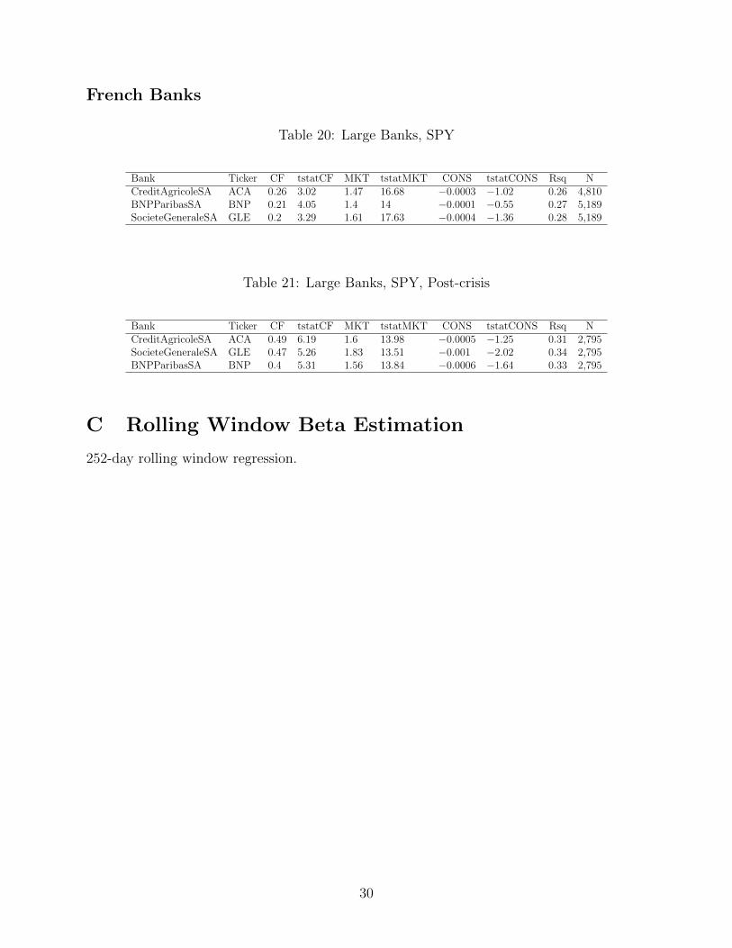
French Banks


Bank Ticker CF tstatCF MKT tstatMKT CONS tstatCONS Rsq NCreditAgricoleSA ACA 0.26 3.02 1.47 16.68 −0.0003 −1.02 0.26 4,810BNPParibasSA BNP 0.21 4.05 1.4 14 −0.0001 −0.55 0.27 5,189SocieteGeneraleSA GLE 0.2 3.29 1.61 17.63 −0.0004 −1.36 0.28 5,189


Bank Ticker CF tstatCF MKT tstatMKT CONS tstatCONS Rsq NCreditAgricoleSA ACA 0.49 6.19 1.6 13.98 −0.0005 −1.25 0.31 2,795SocieteGeneraleSA GLE 0.47 5.26 1.83 13.51 −0.001 −2.02 0.34 2,795BNPParibasSA BNP 0.4 5.31 1.56 13.84 −0.0006 −1.64 0.33 2,795

C Rolling Window Beta Estimation

252-day rolling window regression.

30

U.S. Banks

Figure 17: US Large Banks, SPY

31

Figure 18: US Large Banks, SPY

32

U.K. Banks

Figure 19: UK Large Banks, SPY

2002 2004 2006 2008 2010 2012 2014 2016 2018 2020-2

0

2

CF

Bet

a

BARC:LN

2002 2004 2006 2008 2010 2012 2014 2016 2018 2020-2

0

2

CF

Bet

a

HSBA:LN

2002 2004 2006 2008 2010 2012 2014 2016 2018 2020-2

0

2

CF

Bet

a

LLOY:LN

2002 2004 2006 2008 2010 2012 2014 2016 2018 2020-2

0

2

CF

Bet

a

NWG:LN

2002 2004 2006 2008 2010 2012 2014 2016 2018 2020-2

0

2

CF

Bet

a

STAN:LN

33

Figure 20: UK Large Banks, SPY

2008 2010 2012 2014 2016 2018 20200

0.5

1

1.5

Mar

ket B

eta

000001:CH

2008 2010 2012 2014 2016 2018 2020

0

0.5

1

1.5

Mar

ket B

eta

600000:CH

2008 2010 2012 2014 2016 2018 2020

0

1

2

Mar

ket B

eta

600015:CH

2008 2010 2012 2014 2016 2018 2020

0

0.5

1

1.5

Mar

ket B

eta

600016:CH

2008 2010 2012 2014 2016 2018 2020

0

0.5

1

1.5

Mar

ket B

eta

600036:CH

2010 2012 2014 2016 2018 2020

0

0.5

1

1.5

Mar

ket B

eta

601166:CH

2010 2012 2014 2016 2018 2020

0

0.5

1

Mar

ket B

eta

601169:CH

2012 2013 2014 2015 2016 2017 2018 2019 2020 2021

0

0.5

1

Mar

ket B

eta

601288:CH

2008 2010 2012 2014 2016 2018 2020

0

0.5

1

Mar

ket B

eta

601398:CH

2012 2013 2014 2015 2016 2017 2018 2019 2020 2021

0

0.5

1

1.5

Mar

ket B

eta

601818:CH

34

Canadian Banks

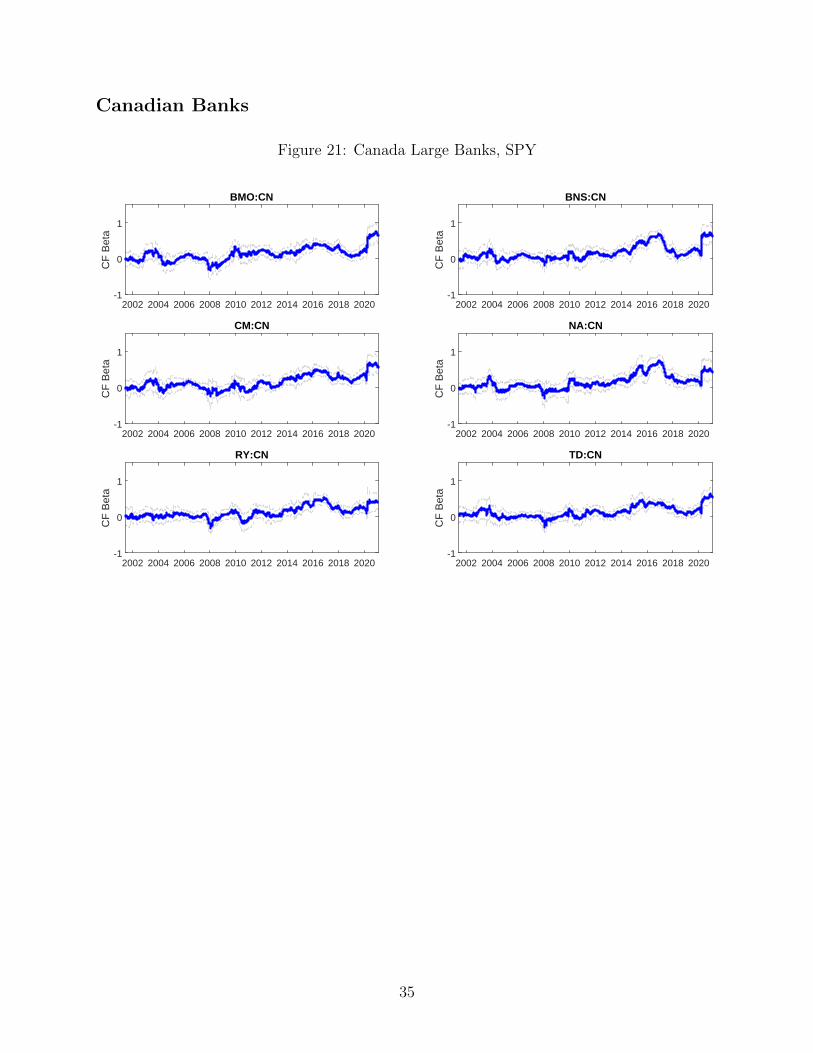
Figure 21: Canada Large Banks, SPY

2002 2004 2006 2008 2010 2012 2014 2016 2018 2020-1

0

1

CF

Bet

a

BMO:CN

2002 2004 2006 2008 2010 2012 2014 2016 2018 2020-1

0

1

CF

Bet

a

BNS:CN

2002 2004 2006 2008 2010 2012 2014 2016 2018 2020-1

0

1

CF

Bet

a

CM:CN

2002 2004 2006 2008 2010 2012 2014 2016 2018 2020-1

0

1

CF

Bet

a

NA:CN

2002 2004 2006 2008 2010 2012 2014 2016 2018 2020-1

0

1

CF

Bet

a

RY:CN

2002 2004 2006 2008 2010 2012 2014 2016 2018 2020-1

0

1

CF

Bet

a

TD:CN

35

Figure 22: Canada Large Banks, SPY

2002 2004 2006 2008 2010 2012 2014 2016 2018 20200

2

4

Mar

ket B

eta

BMO:CN

2002 2004 2006 2008 2010 2012 2014 2016 2018 20200

2

4

Mar

ket B

eta

BNS:CN

2002 2004 2006 2008 2010 2012 2014 2016 2018 20200

2

4

Mar

ket B

eta

CM:CN

2002 2004 2006 2008 2010 2012 2014 2016 2018 20200

2

4

Mar

ket B

eta

NA:CN

2002 2004 2006 2008 2010 2012 2014 2016 2018 20200

2

4

Mar

ket B

eta

RY:CN

2002 2004 2006 2008 2010 2012 2014 2016 2018 20200

2

4

Mar

ket B

eta

TD:CN

Japanese Banks

Figure 23: Japan Large Banks, SPY

2004 2006 2008 2010 2012 2014 2016 2018 2020-1

-0.5

0

0.5

1

1.5

CF

Bet

a

8306:JP

2004 2006 2008 2010 2012 2014 2016 2018 2020-1

-0.5

0

0.5

1

1.5

CF

Bet

a

8316:JP

2006 2008 2010 2012 2014 2016 2018 2020-1

-0.5

0

0.5

1

1.5

CF

Bet

a

8411:JP

36

Figure 24: Japan Large Banks, SPY

2004 2006 2008 2010 2012 2014 2016 2018 20200

1

2

3

4

Mar

ket B

eta

8306:JP

2004 2006 2008 2010 2012 2014 2016 2018 20200

1

2

3

4

Mar

ket B

eta

8316:JP

2006 2008 2010 2012 2014 2016 2018 20200

1

2

3

4

Mar

ket B

eta

8411:JP

French Banks

Figure 25: French Large Banks, SPY

2004 2006 2008 2010 2012 2014 2016 2018 2020-1

-0.5

0

0.5

1

1.5

CF

Bet

a

ACA:FP

2002 2004 2006 2008 2010 2012 2014 2016 2018 2020-1

-0.5

0

0.5

1

1.5

CF

Bet

a

BNP:FP

2002 2004 2006 2008 2010 2012 2014 2016 2018 2020-1

-0.5

0

0.5

1

1.5

CF

Bet

a

GLE:FP

37

Figure 26: French Large Banks, SPY

2004 2006 2008 2010 2012 2014 2016 2018 20200

1

2

3

4

Mar

ket B

eta

ACA:FP

2002 2004 2006 2008 2010 2012 2014 2016 2018 20200

1

2

3

4

Mar

ket B

eta

BNP:FP

2002 2004 2006 2008 2010 2012 2014 2016 2018 20200

1

2

3

4

Mar

ket B

eta

GLE:FP

38

D DCB Model Estimateion

U.S. Banks

Figure 27: Climate Beta of U.S. Banks

39

Figure 28: Market Beta of U.S. Banks

40

U.K. Banks

Figure 29: Climate Beta (γ1it + γ2it), U.K. Banks

2005 2010 2015 2020

-1

0

1

Clim

ate

Bet

a

BARC:LN

2005 2010 2015 2020

-0.5

0

0.5

1

Clim

ate

Bet

a

HSBA:LN

2005 2010 2015 2020-1

0

1

Clim

ate

Bet

a

LLOY:LN

2005 2010 2015 2020

-1

0

1

Clim

ate

Bet

a

NWG:LN

2005 2010 2015 2020

-0.5

0

0.5

1

Clim

ate

Bet

a

STAN:LN

41

Figure 30: Market Beta (β1it + β2it), U.K. Banks

2005 2010 2015 20200

1

2

3

Mar

ket B

eta

BARC:LN

2005 2010 2015 20200

1

2

Mar

ket B

eta

HSBA:LN

2005 2010 2015 20200

1

2

3

Mar

ket B

eta

LLOY:LN

2005 2010 2015 20200

1

2

3

Mar

ket B

eta

NWG:LN

2005 2010 2015 20200

1

2

3

Mar

ket B

eta

STAN:LN

42

Canadian Banks

Figure 31: Climate Beta (γ1it + γ2it), Canadian Banks, SPY

2005 2010 2015 2020

-0.5

0

0.5

1

Clim

ate

Bet

a

BMO:CN

2005 2010 2015 2020

-0.5

0

0.5

1

Clim

ate

Bet

a

BNS:CN

2005 2010 2015 2020

-0.5

0

0.5

1

Clim

ate

Bet

a

CM:CN

2005 2010 2015 2020

-0.5

0

0.5

1

Clim

ate

Bet

a

NA:CN

2005 2010 2015 2020

-0.5

0

0.5

1

Clim

ate

Bet

a

RY:CN

2005 2010 2015 2020

-0.5

0

0.5

1

Clim

ate

Bet

a

TD:CN

43

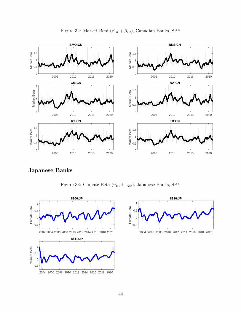
Figure 32: Market Beta (β1it + β2it), Canadian Banks, SPY

2005 2010 2015 20200

0.5

1

1.5

Mar

ket B

eta

BMO:CN

2005 2010 2015 20200

0.5

1

1.5

Mar

ket B

eta

BNS:CN

2005 2010 2015 20200

1

2

Mar

ket B

eta

CM:CN

2005 2010 2015 20200

0.5

1

1.5

Mar

ket B

eta

NA:CN

2005 2010 2015 20200

0.5

1

1.5

Mar

ket B

eta

RY:CN

2005 2010 2015 20200

0.5

1

1.5M

arke

t Bet

a

TD:CN

Japanese Banks

Figure 33: Climate Beta (γ1it + γ2it), Japanese Banks, SPY

2002 2004 2006 2008 2010 2012 2014 2016 2018 2020

-0.5

0

0.5

1

Clim

ate

Bet

a

8306:JP

2004 2006 2008 2010 2012 2014 2016 2018 2020

-0.5

0

0.5

1

Clim

ate

Bet

a

8316:JP

2004 2006 2008 2010 2012 2014 2016 2018 2020

-0.5

0

0.5

1

Clim

ate

Bet

a

8411:JP

44

Figure 34: Market Beta (β1it + β2it), Japanese Large Banks, SPY

2002 2004 2006 2008 2010 2012 2014 2016 2018 20200

0.5

1

1.5

2

Mar

ket B

eta

8306:JP

2004 2006 2008 2010 2012 2014 2016 2018 20200

1

2

Mar

ket B

eta

8316:JP

2004 2006 2008 2010 2012 2014 2016 2018 20200

1

2

Mar

ket B

eta

8411:JP

French Banks

Figure 35: Climate Beta (γ1it + γ2it), French Banks, SPY

2004 2006 2008 2010 2012 2014 2016 2018 2020

-0.5

0

0.5

1

Clim

ate

Bet

a

ACA:FP

2005 2010 2015 2020

-0.5

0

0.5

1

1.5

Clim

ate

Bet

a

BNP:FP

2005 2010 2015 2020

-0.5

0

0.5

1

1.5

Clim

ate

Bet

a

GLE:FP

45

Figure 36: Market Beta (β1it + β2it), Japanese Large Banks, SPY

2004 2006 2008 2010 2012 2014 2016 2018 20200

1

2

3

Mar

ket B

eta

ACA:FP

2005 2010 2015 20200

1

2

3

Mar

ket B

eta

BNP:FP

2005 2010 2015 20200

1

2

3

4

Mar

ket B

eta

GLE:FP

46

E CRISK during the year 2020

Canadian Banks

Figure 37: Climate SRISK, Canadian Large Banks, SPY


10

20

30

40

50

60

70

CR

ISK

($b

io)


Table 22: Climate SRISK Decomposition

SRISK(t) is Climate SRISK at the end of the first half of 2020, and SRISK(t-1) is ClimateSRISK at the beginning of year 2020. dSRISK= SRISK(t)-SRISK(t-1) is the change inClimate SRISK during the first half of 2020. dDEBT is the contribution of the firm’s debtto Climate SRISK. dEQUITY is the contribution of the firm’s equity position on ClimateSRISK. dRISK is the contribution of increase in volatility or correlation to Climate SRISK.

Bank CRISK(t-1) CRISK(t) dCRISK dDEBT dEQUITY dRISKBMO:CN 10.9548 21.3558 10.401 8.4648 2.4641 -0.60693BNS:CN 4.9275 21.8717 16.9442 6.7029 4.3385 5.6732CM:CN 10.7674 18.5225 7.7551 9.1872 -0.50982 -1.1118NA:CN -0.60828 4.2192 4.8275 3.9944 0.19835 0.74084RY:CN -7.1409 14.3521 21.4929 16.5501 1.551 2.6546TD:CN 4.9256 31.6962 26.7706 22.0538 3.0312 0.93249

47

Japanese Banks

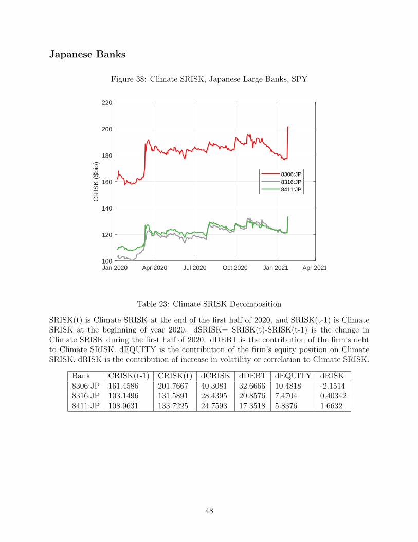
Figure 38: Climate SRISK, Japanese Large Banks, SPY


120

140

160

180

200

220C

RIS

K (

$bio

)

8306:JP8316:JP8411:JP



Bank CRISK(t-1) CRISK(t) dCRISK dDEBT dEQUITY dRISK8306:JP 161.4586 201.7667 40.3081 32.6666 10.4818 -2.15148316:JP 103.1496 131.5891 28.4395 20.8576 7.4704 0.403428411:JP 108.9631 133.7225 24.7593 17.3518 5.8376 1.6632

48

French Banks

Figure 39: Climate SRISK, Japanese Large Banks, SPY


100

120

140

160

180

200

220C

RIS

K (

$bio

)

ACA:FPBNP:FPGLE:FP



Bank CRISK(t-1) CRISK(t) dCRISK dDEBT dEQUITY dRISKACA:FP 118.5924 159.0539 40.4615 28.6049 6.7488 4.5746BNP:FP 123.3387 200.166 76.8273 54.8439 12.2204 9.0397GLE:FP 94.6865 128.1424 33.4559 19.4558 7.8485 5.7192

49

F Stressed vs. Non-stressed CRISK

Difference between CRISK and non-stressed CRISK:

(1 − k)(1 − exp

(βClimate log(1 − θ)

))W

Figure 40: US Banks

2005 2010 2015 20200

50

100

CR

ISK

Diff

($b

io)

BAC:US

2005 2010 2015 20200

50

100

CR

ISK

Diff

($b

io)

BK:US

2005 2010 2015 20200

50

100

CR

ISK

Diff

($b

io)

C:US

2005 2010 2015 20200

50

100C

RIS

K D

iff (

$bio

)

COF:US

2005 2010 2015 20200

50

100

CR

ISK

Diff

($b

io)

GS:US

2005 2010 2015 20200

50

100

CR

ISK

Diff

($b

io)

JPM:US

2005 2010 2015 20200

50

100

CR

ISK

Diff

($b

io)

MS:US

2005 2010 2015 20200

50

100

CR

ISK

Diff

($b

io)

PNC:US

2005 2010 2015 20200

50

100

CR

ISK

Diff

($b

io)

USB:US

2005 2010 2015 20200

50

100

CR

ISK

Diff

($b

io)

WFC:US

50

Difference between CRISK and non-stressed CRISK:

(1 − k)(1 − exp


))W

when the climate factor is 0.3 XLE + 0.7 KOL.

Figure 41: US Banks

2005 2010 2015 20200

50

100

CR

ISK

Diff

($b

io)

BAC:US

2005 2010 2015 20200

50

100

CR

ISK

Diff

($b

io)

BK:US

2005 2010 2015 20200

50

100

CR

ISK

Diff

($b

io)

C:US

2005 2010 2015 20200

50

100

CR

ISK

Diff

($b

io)

COF:US

2005 2010 2015 20200

50

100

CR

ISK

Diff

($b

io)

GS:US

2002 2004 2006 2008 2010 2012 2014 2016 2018 20200

50

100

CR

ISK

Diff

($b

io)

JPM:US

2005 2010 2015 20200

50

100

CR

ISK

Diff

($b

io)

MS:US

2005 2010 2015 20200

50

100

CR

ISK

Diff

($b

io)

PNC:US

2005 2010 2015 20200

50

100

CR

ISK

Diff

($b

io)

USB:US

2005 2010 2015 20200

50

100

CR

ISK

Diff

($b

io)

WFC:US

51

Figure 42: US Banks

Difference between CRISK and non-stressed CRISK scaled by equity:

(1 − k)(1 − exp


))

2005 2010 2015 20200

0.2

0.4

Fra

ctio

n of

Equ

ity

BAC:US

2005 2010 2015 20200

0.1

0.2

0.3

Fra

ctio

n of

Equ

ity

BK:US

2005 2010 2015 20200

0.2

0.4

Fra

ctio

n of

Equ

ity

C:US

2005 2010 2015 20200

0.2

0.4

Fra

ctio

n of

Equ

ity

COF:US

2005 2010 2015 20200

0.1

0.2

Fra

ctio

n of

Equ

ity

GS:US

2005 2010 2015 20200

0.1

0.2

0.3

Fra

ctio

n of

Equ

ity

JPM:US

2005 2010 2015 20200

0.1

0.2

0.3

Fra

ctio

n of

Equ

ity

MS:US

2005 2010 2015 20200

0.1

0.2

0.3

Fra

ctio

n of

Equ

ity

PNC:US

2005 2010 2015 20200

0.2

0.4

Fra

ctio

n of

Equ

ity

USB:US

2005 2010 2015 20200

0.2

0.4

Fra

ctio

n of

Equ

ity

WFC:US

52

Figure 43: Canadian Banks

2005 2010 2015 2020-40

-20

0

20

40

60

CR

ISK

($b

io)

BMO:CN


2005 2010 2015 2020-40

-20

0

20

40

60

CR

ISK

($b

io)

BNS:CN


2005 2010 2015 2020-40

-20

0

20

40

60

CR

ISK

($b

io)

CM:CN


2005 2010 2015 2020-40

-20

0

20

40

60

CR

ISK

($b

io)

NA:CN


2005 2010 2015 2020-40

-20

0

20

40

60

CR

ISK

($b

io)

RY:CN


2005 2010 2015 2020-40

-20

0

20

40

60

CR

ISK

($b

io)

TD:CN


Figure 44: Japanese Banks

2004 2006 2008 2010 2012 2014 2016 2018 2020

0

100

200

CR

ISK

($b

io)

8306:JP


2004 2006 2008 2010 2012 2014 2016 2018 2020

0

100

200

CR

ISK

($b

io)

8316:JP


2004 2006 2008 2010 2012 2014 2016 2018 2020

0

100

200

CR

ISK

($b

io)

8411:JP


53

Figure 45: French Banks

2004 2006 2008 2010 2012 2014 2016 2018 2020

50

100

150

200

CR

ISK

($b

io)

ACA:FP


2005 2010 2015 2020

50

100

150

200

CR

ISK

($b

io)

BNP:FP


2005 2010 2015 2020

50

100

150

200

CR

ISK

($b

io)

GLE:FP


G Global Banks

Figure 46: US and UK Banks Exposure to Oil and Gas

Source: Bloomberg Loan League Table History11

0

5

10

15

20

Loan

US

D b

io

2005q1 2010q1 2015q1 2020q1qdate

Bank of America BarclaysBofA Securities Capital One FinancialCiti Goldman SachsHSBC JP MorganLloyds Bank Morgan StanleyPNC Financial Services Group Inc RBSStandard Chartered Bank US BancorpWells Fargo

54

Table 25: Top 50 Global Banks by Exposure to Oil and Gas

LoanRecent is loan amount in USD billion during Jan 2019 - June 2020.Source: Bloomberg Loan League Table History

bank Country LoanRecent ShrRecent CumShr

1 JP Morgan US 42.588 0.08 0.082 Wells Fargo US 42.168 0.08 0.153 BNP Paribas France 37.926 0.07 0.224 BofA Securities US 32.521 0.06 0.285 Citi US 31.568 0.06 0.346 RBC Capital Markets Canada 25.598 0.05 0.397 TD Securities Canada 24.986 0.05 0.438 Mitsubishi UFJ Financial Group Inc Japan 22.636 0.04 0.479 Mizuho Financial Japan 22.174 0.04 0.5110 Sumitomo Mitsui Financial Japan 20.035 0.04 0.5511 Scotiabank Canada 19.292 0.04 0.5912 BMO Capital Markets Canada 19.2 0.04 0.6213 HSBC UK 18.44 0.03 0.6614 CIBC Canada 15.913 0.03 0.6815 Societe Generale France 13.75 0.03 0.7116 Credit Agricole CIB France 11.76 0.02 0.7317 Barclays UK 11.211 0.02 0.7518 National Bank Financial Inc Canada 8.779 0.02 0.7719 ING Groep Netherlands 7.888 0.01 0.7820 First Abu Dhabi Bank PJSC UAE 7.61 0.01 0.821 Bank of China China 7.293 0.01 0.8122 Natixis France 7.089 0.01 0.8223 Banco Santander Spain 7.083 0.01 0.8324 State Bank of India India 6.222 0.01 0.8525 Goldman Sachs US 5.361 0.01 0.8626 Standard Chartered Bank UK 5.284 0.01 0.8727 UniCredit Italy 5.057 0.01 0.8728 Credit Suisse Switzerland 4.949 0.01 0.8829 United Overseas Bank Singapore 4.813 0.01 0.8930 Deutsche Bank Germany 3.886 0.01 0.931 ANZ Banking Group Australia 3.504 0.01 0.9132 PNC Financial Services Group Inc US 3.212 0.01 0.9133 DBS Group Singapore 3.155 0.01 0.9234 Oversea Chinese Banking Corp Singapore 3.079 0.01 0.9235 Westpac Banking Australia 2.814 0.01 0.9336 DNB ASA Norway 2.473 0.00 0.9337 Jefferies US 2.442 0.00 0.9438 Rabobank Netherlands 2.403 0.00 0.9439 Banco Bilbao Vizcaya Argentaria Spain 1.861 0.00 0.9440 Commerzbank Germany 1.73 0.00 0.9541 African Export Import Bank Egypt 1.656 0.00 0.9542 US Bancorp US 1.651 0.00 0.9543 Industrial Comm Bank of China China 1.62 0.00 0.9644 Nordea Finland 1.534 0.00 0.9645 Citizens Financial Group Inc US 1.512 0.00 0.9646 Lloyds Bank UK 1.4 0.00 0.9747 Commonwealth Bank Australia Australia 1.251 0.00 0.9748 Capital One Financial US 1.247 0.00 0.9749 UBS Switzerland 1.019 0.00 0.9750 National Australia Bank Australia 0.9878754 0.00 0.97

55

Additional Robustness Results

∆βClimateit = a+ b ·GOLoansi,t−1 + εit

where βClimateit is bank i’s time-averaged dynamically-estimated daily climate beta during

quarter t. GOLoansit is bank i’s new syndicated loans to the oil and gas industry (scaledby assets) in quarter t. The full sample includes 14 banks (9 U.S. banks and 5 U.K. banks)from the first quarter of 2008 to the second quarter of 2020. Standard errors are clusteredby banks.

Table 26: Climate Beta and Gas & Oil Loan Exposure

(1) (2) (3) (4)US UK FullSample FullSample

OilGasLoan(Lag) 0.00632∗ 0.0791∗∗∗ 0.0109∗ 0.0105∗

(1.94) (10.34) (1.97) (2.07)

Constant 0.00745∗∗∗ 0.0434∗∗∗ 0.00961∗∗∗ 0.0795∗∗∗

(4.41) (6.03) (4.64) (5.40)YearFE N N N YCtryFE N N N YN 441 245 686 686RSqr 0.00223 0.0115 0.00213 0.0497

t statistics in parentheses∗ p < 0.1, ∗∗ p < 0.05, ∗∗∗ p < 0.01

56

Documents

Climate Stress Testing - newyorkfed.org