Embed Size (px)
Citation preview
Working Paper No. 2018-3May 30, 2018
Who are Driving Electric Vehicles?An analysis of factors that affect EV
adoption in Hawaii
by
Makena Coffman, Scott F. Allen, andSherilyn Wee
UNIVERSITY OF HAWAI‘ I AT MANOA
2424 MAILE WAY, ROOM 540 • HONOLULU, HAWAI‘ I 96822
WWW.UHERO.HAWAII .EDU
WORKING PAPERS ARE PRELIMINARY MATERIALS CIRCULATED TO STIMULATE
DISCUSSION AND CRITICAL COMMENT. THE VIEWS EXPRESSED ARE THOSE OF
THE INDIVIDUAL AUTHORS.
Who are Driving Electric Vehicles? An analysis of factors that affect EV adoption in Hawaii
Makena Coffman* Professor, Urban and Regional Planning
Research Fellow, UHERO University of Hawaii at Manoa [email protected]
(808) 956-2890
Scott Allen MA Candidate
Urban and Regional Planning University of Hawaii at Manoa
Sherilyn Wee PhD, Economics
Affiliate Researcher, UHERO [email protected]
May 29, 2018
*Corresponding Author

2
Acknowledgements We thank the State of Hawaii Division of Consumer Advocacy for their financial support of this project and the University of Hawaii Economic Research Organization for their administrative support.
3
Abstract Electric vehicles (EVs) have the potential to reduce local air pollution as well as greenhouse gas emissions, assuming they are predominantly powered with renewable energy. Upon their reintroduction to the mass vehicle market in 2010, President Obama set a goal of having a million on the road in the U.S. by 2015. Similarly, in Hawaii, the Hawaii Clean Energy Initiative target was to have 10,000 EVs on the road by 2015 and 40,000 by 2020. Despite policy support, actual rates of EV adoption have fallen substantially short of stated goals. By the end of 2017, there were about 770,00 EVs within the U.S., with 6,700 of these in Hawaii. This study uses data on EV registrations by zipcode in Hawaii to analyze a variety of demographic and transportation factors that might affect EV adoption. We find that, after controlling for population and gasoline prices, higher income zipcodes are associated with higher levels of EV adoption – where an increase of $10,000 in median income is associated with an additional 6 EVs within the 2010-2016 study time period (where the average zipcode in our sample had 68 EVs in 2016). When educational attainment is measured, we find that a 1% increase in the number of people with at least a bachelor’s degree increases zipcode EV adoption by about 76. We find some evidence that gender can matter, similar to other studies that find that men are more likely to adopt EVs. The effect of age seems to be more robust, where we find that for every 1-year increase from the average zipcode’s median age, there are 1 to 2 more EVs. Most notably, we find that commute time affects EV adoption in Hawaii – which is somewhat surprising given the relatively limited travel distances of an island geography. We find that a 1% increase in the prevalence of commute times greater than forty-five minutes within a zipcode, likely meaning they are farther from the central business district, is associated with 37 fewer EVs relative to those with a commute time under forty-five minutes. This finding holds even when looking at the island of Oahu alone, which has the majority of the state’s population as well as the majority of EVs. The island is about forty-four miles long, far less distance than the range offered by most EVs. This suggests that there may be strong risk-aversion associated with EV range anxiety as well as prompts further study of the effect of trip-chaining on EV purchase decisions.
4
Introduction Electric vehicles (EVs) have the capability to dramatically increase fuel economy, reduce local air pollution and, depending on how the power is generated, decrease greenhouse gas (GHG) emissions within the transport sector (Coffman et al., 2016a; Onat et al., 2015; Hawkins et al, 2012; Samaras and Meisterling, 2008). Now nearly every major vehicle manufacturer has an electric model. There are policy efforts in Hawaii towards adoption of renewable energy and alternative transportation. The State of Hawaii has an aggressive renewable portfolio standard (RPS) for the power sector, aiming to achieve 40% of net sales of electricity through renewable sources by the year 2030, 70% by 2040 and 100% by 2045. The Hawaii Clean Energy Initiative had set an initial target to have 10,000 EVs on the road by 2015 and 40,000 by 2020. More recently, Hawaii’s four county mayors committed to a shared goal of 100% of ground transportation from renewable fuel by 2045. In response to the emerging EV market and in light of stated goals, the State has made concerted efforts to support EV adoption. In addition to the federal purchase subsidy of up to $2,500 per vehicle, the State of Hawaii offered a vehicle purchase subsidy of $4,500 and a home charger subsidy of $500 to early adopters between 2010 and 2012. EVs are granted a number of in-kind incentives including access to HOV lanes, designated and free parking at public lots and meters. In 2012, the legislature passed a law that mandates parking lots with 100 stalls or more to provide a charging station (Lincoln, 2013). Despite strong policy support, however, EV adoption rates have fallen short. By the end of 2017, there were roughly 6,700 EVs registered in Hawaii (DBEDT, 2018). This study aims to provide understanding of the determinants of EV adoption in the case of Hawaii. We leverage differences in zipcode level demographic and transportation habits to identify differences in EV purchases through 2016. We find that demographic factors like higher income are associated with more EV registrations within a zipcode. In addition, factors related to urban form embodied by duration of commute also matter. We find that households with a commute time greater than 45 minutes are associated with a decrease in EV adoption relative to households with a shorter commute time. Factors that Affect EV Adoption There is a robust and growing literature on the factors that affect EV adoption worldwide. Coffman et al. (2016b) review fifty studies that address the factors that affect EV adoption. They group studies based on papers that discuss factors internal to EVs, like battery performance, and those that discuss factors that are external to EVs, like fuel prices. Important internal characteristics that affect the purchase of EVs include vehicle ownership costs, driving range and charging time (Carley et al. 2013; Dimitropoulos et al., 2013; Graham-Rowe et al., 2012; Hidrue et al., 2011). Important external variables include relative fuel prices, availability of charging stations, consumer characteristics and public visibility/social norms. There is a plethora of simulation-based studies that show the important of relative fuel prices in EV adoption (Al-Alawi and Bradley, 2013; Prud’homme and Koning, 2012; Tseng et al., 2013; Wu et al., 2014). However, the limited empirical work that exists show mixed results. Sierzchula et al. (2014) look at 30 countries vehicle markets in 2012 and find that fuel price is not a significant predictor of EV market share. This is counter to work on hybrid electric vehicles (HEV) that suggest fuel prices are a key driver of HEV adoption (Beresteanu and Li, 2011; Diamond, 2009; Gallagher and Muehlegger, 2011). The availability of charging station infrastructure is shown to be critically important to EV adoption (Bakker et al, 2014; Campbell et al., 2012; Egbue and Long, 2012; Lopes et al., 2014; Schroder and Traber, 2012). However, charging infrastructure is
5
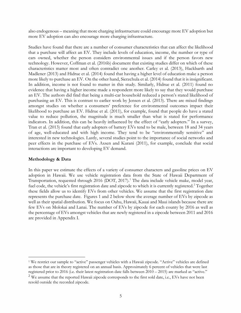
also endogenous – meaning that more charging infrastructure could encourage more EV adoption but more EV adoption can also encourage more charging infrastructure. Studies have found that there are a number of consumer characteristics that can affect the likelihood that a purchase will affect an EV. They include levels of education, income, the number or type of cars owned, whether the person considers environmental issues and if the person favors new technology. However, Coffman et al. (2016b) document that existing studies differ on which of these characteristics matter most and often contradict one another. Carley et al. (2013), Hackbarth and Madlener (2013) and Hidrue et al. (2014) found that having a higher level of education make a person more likely to purchase an EV. On the other hand, Sierzchula et al. (2014) found that it is insignificant. In addition, income is not found to matter in this study. Similarly, Hidrue et al. (2011) found no evidence that having a higher income made a respondent more likely to say that they would purchase an EV. The authors did find that being a multi-car household reduced a person’s stated likelihood of purchasing an EV. This is contrast to earlier work by Jensen et al. (2013). There are mixed findings amongst studies on whether a consumers’ preference for environmental outcomes impact their likelihood to purchase an EV. Hidrue et al. (2011), for example, found that people do have a stated value to reduce pollution, the magnitude is much smaller than what is stated for performance indicators. In addition, this can be heavily influenced by the effect of “early adopters.” In a survey, Tran et al. (2013) found that early adopters of battery EVs tend to be male, between 18 and 34 years of age, well-educated and with high income. They tend to be “environmentally sensitive” and interested in new technologies. Lastly, several studies point to the importance of social networks and peer effects in the purchase of EVs. Axsen and Kurani (2011), for example, conclude that social interactions are important to developing EV demand. Methodology & Data In this paper we estimate the effects of a variety of consumer characters and gasoline prices on EV adoption in Hawaii. We use vehicle registration data from the State of Hawaii Department of Transportation, requested through 2016 (DOT, 2017).1 The data include vehicle make, model year, fuel code, the vehicle’s first registration date and zipcode to which it is currently registered.2 Together these fields allow us to identify EVs from other vehicles. We assume that the first registration date represents the purchase date. Figures 1 and 2 below show the average number of EVs by zipcode as well as their spatial distribution. We focus on Oahu, Hawaii, Kauai and Maui islands because there are few EVs on Molokai and Lanai. The number of EVs by zipcode for each county by 2016 as well as the percentage of EVs amongst vehicles that are newly registered in a zipcode between 2011 and 2016 are provided in Appendix I.
1 We restrict our sample to “active” passenger vehicles with a Hawaii zipcode. “Active” vehicles are defined as those that are in theory registered on an annual basis. Approximately 6 percent of vehicles that were last registered prior to 2016 (i.e. their latest registration date falls between 2010 – 2015) are marked as “active.” 2 We assume that the reported Hawaii zipcode corresponds to the first sold date, i.e., EVs have not been resold outside the recorded zipcode.
6
Figure 1. Average Number of EVs per Hawaii Zipcode, 2011-2016
7
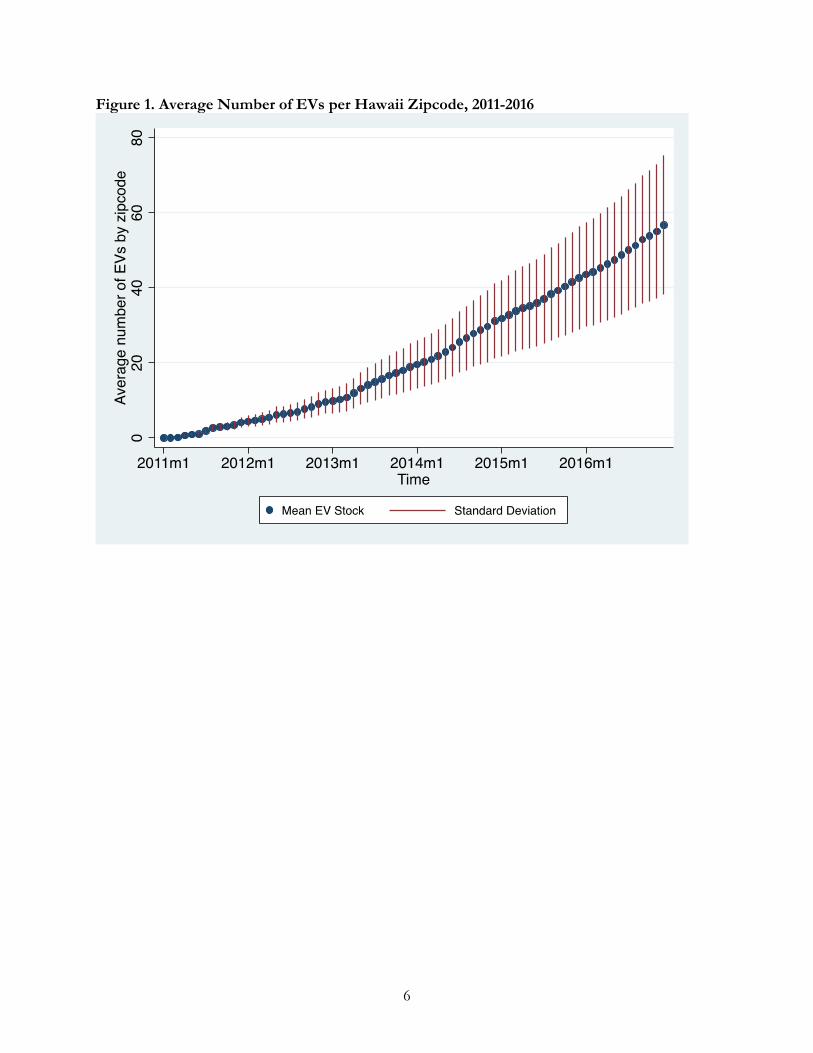
Figure 2. EV Registrations by Zipcode, 2016
By the end of 2016, there are an average of 57 EVs per zipcode, though this is far from equally spatially distributed. The highest number of EVs are on Oahu, where Kailua/Kaneohe and urban Honolulu have the highest levels of adoption. Having the data identified at the zipcode allows us to use zipcode level census data for consumer characteristics. Our approach is to statistically leverage the variation in consumer demographic and travel characteristics to explain the variation in EV registration by zipcodes, accounting for changes in gasoline prices. From the review of the literature coupled with available census data, we identify income, gender, mode and duration of commute, and owning multiple vehicles as the important socio-economic and travel behavior related factors that might affect owning an EV. We also control for zipcode population and county gasoline prices. This is shown in Equation 1 below. We rely on zipcode-level demographic data from the 2010 Census where available, and supplement this with the American Community Survey (ACS). The ACS data at the zipcode-level is only available as 5-year estimates, and therefore coupled with the 2010 Census data, restricts the demographic variables to a single zipcode value throughout our sample period.
8
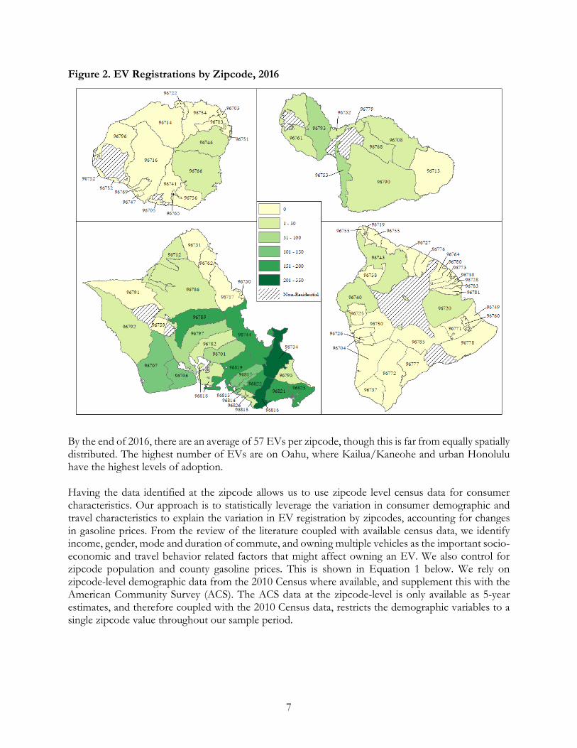
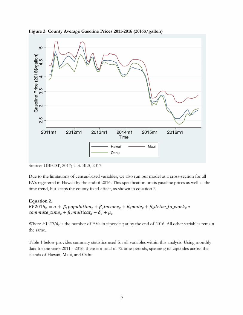
Equation 1. 𝐸𝐸𝐸𝐸𝑧𝑧𝑧𝑧 = 𝛼𝛼 + 𝛽𝛽1𝑝𝑝𝑝𝑝𝑝𝑝𝑝𝑝𝑝𝑝𝑝𝑝𝑝𝑝𝑝𝑝𝑝𝑝𝑝𝑝𝑧𝑧 + 𝛽𝛽2𝑝𝑝𝑝𝑝𝑖𝑖𝑝𝑝𝑖𝑖𝑖𝑖𝑧𝑧 + 𝛽𝛽3𝑖𝑖𝑝𝑝𝑝𝑝𝑖𝑖𝑧𝑧 + 𝛽𝛽4𝑑𝑑𝑟𝑟𝑝𝑝𝑟𝑟𝑖𝑖_𝑝𝑝𝑝𝑝_𝑤𝑤𝑝𝑝𝑟𝑟𝑤𝑤𝑧𝑧 ∗𝑖𝑖𝑝𝑝𝑖𝑖𝑖𝑖𝑝𝑝𝑝𝑝𝑖𝑖_𝑝𝑝𝑝𝑝𝑖𝑖𝑖𝑖𝑧𝑧 + 𝛽𝛽7𝑖𝑖𝑝𝑝𝑝𝑝𝑝𝑝𝑝𝑝𝑖𝑖𝑝𝑝𝑟𝑟𝑧𝑧 + 𝛽𝛽8𝑔𝑔𝑝𝑝𝑔𝑔𝑝𝑝𝑝𝑝𝑝𝑝𝑝𝑝𝑖𝑖𝑐𝑐𝑧𝑧 + 𝛿𝛿𝑐𝑐𝑝𝑝 + 𝜎𝜎𝑧𝑧 + 𝜇𝜇𝑧𝑧𝑧𝑧 EVzt is the number of EVs in zipcode z at time t (end of the month for that year). Populationz is the population within zipcode z (U.S. Census Bureau, 2010). Incomez is the median income (in $10,000s) in zipcode z between 2011 – 2015 (ACS, 2015a). We run a specification without income and instead include educationz, which is the percentage of the population over 25 years of age in zipcode z with a college diploma between 2011 – 2015 (ACS, 2015b). The variables incomez and educationz are highly correlated with a correlation coefficient of 0.51. The variable malez is the percentage of males in zipcode z in 2010 (U.S. Census Bureau, 2010). Drive_to_work is the percentage of people in zipcode z that drive to work, in contrast to the alternatives that include bus/transit, carpooling, biking, walking or working at home (ACS, 2015c). Drive_to_work is interacted with commute_timez, which is the average number of minutes that it takes to commute to work in a private vehicle in zipcode z (ACS, 2015d). Commute_timez is diced into three bins: the percentage of commutes less than 20 minutes, 20-44 minutes, and greater than 45 minutes. We interact these two terms because it is commute times in private vehicles that would affect EV adoption, not commute times by, for example, bus. As a sensitivity analysis, we also run the regression without this interaction and dropping drive_to_work. Multi-carz is the percentage of households within zipcode z that have two or more vehicles (ACS, 2015d). Because this is highly correlated with drive_to_work with a correlation coefficient of 0.66, we run a specification that drops multi-carz. Gasolinect is the price of gasoline in county c at time t (DBEDT, 2017). 𝛿𝛿𝑐𝑐𝑝𝑝 is a county time trend that is intended to pick up county-specific time-varying differences that follow a linear trend, such as the build out of charging infrastructure.3 𝜎𝜎𝑧𝑧 are month-year fixed-effects that control for state-level trends and shocks that may influence EV adoption. 𝜇𝜇𝑧𝑧𝑧𝑧 is the error term (with robust standard errors). Though we know from prior studies that both gasoline and electricity prices are important to a consumer’s decision to purchase an EV, in Hawaii both prices are strongly correlated (correlation coefficient = 0.62) because oil is the main fuel for electricity generation (DBEDT, 2017). Thus, we omit electricity prices and include only gasoline prices at the county level (DBEDT, 2017).4 Gasoline prices are not readily available for Kauai, and this restricts our analysis to the other three islands, as shown in Figure 3.
3 We collected data on the number of charging stations over time in each county. While absolute values differ substantially by county, the cumulative number of charging stations in each follows a linear trend. As such, charging infrastructure can be reasonably captured by a county-specific time trend within the regression specification. This is preferred over modeling charging infrastructure separately due to endogeneity. 4 Prices are adjusted to 2016$ using the Honolulu Consumer Price Index (CPI) (U.S. BLS, 2017).
9
Figure 3. County Average Gasoline Prices 2011-2016 (2016$/gallon)
Source: DBEDT, 2017; U.S. BLS, 2017. Due to the limitations of census-based variables, we also run our model as a cross-section for all EVs registered in Hawaii by the end of 2016. This specification omits gasoline prices as well as the time trend, but keeps the county fixed-effect, as shown in equation 2. Equation 2. 𝐸𝐸𝐸𝐸2016𝑧𝑧 = 𝛼𝛼 + 𝛽𝛽1𝑝𝑝𝑝𝑝𝑝𝑝𝑝𝑝𝑝𝑝𝑝𝑝𝑝𝑝𝑝𝑝𝑝𝑝𝑝𝑝𝑧𝑧 + 𝛽𝛽2𝑝𝑝𝑝𝑝𝑖𝑖𝑝𝑝𝑖𝑖𝑖𝑖𝑧𝑧 + 𝛽𝛽3𝑖𝑖𝑝𝑝𝑝𝑝𝑖𝑖𝑧𝑧 + 𝛽𝛽4𝑑𝑑𝑟𝑟𝑝𝑝𝑟𝑟𝑖𝑖_𝑝𝑝𝑝𝑝_𝑤𝑤𝑝𝑝𝑟𝑟𝑤𝑤𝑧𝑧 ∗𝑖𝑖𝑝𝑝𝑖𝑖𝑖𝑖𝑝𝑝𝑝𝑝𝑖𝑖_𝑝𝑝𝑝𝑝𝑖𝑖𝑖𝑖𝑧𝑧 + 𝛽𝛽7𝑖𝑖𝑝𝑝𝑝𝑝𝑝𝑝𝑝𝑝𝑖𝑖𝑝𝑝𝑟𝑟𝑧𝑧 + 𝛿𝛿𝑐𝑐 + 𝜇𝜇𝑧𝑧 Where EV2016z is the number of EVs in zipcode z at by the end of 2016. All other variables remain the same. Table 1 below provides summary statistics used for all variables within this analysis. Using monthly data for the years 2011 - 2016, there is a total of 72 time-periods, spanning 65 zipcodes across the islands of Hawaii, Maui, and Oahu.
10
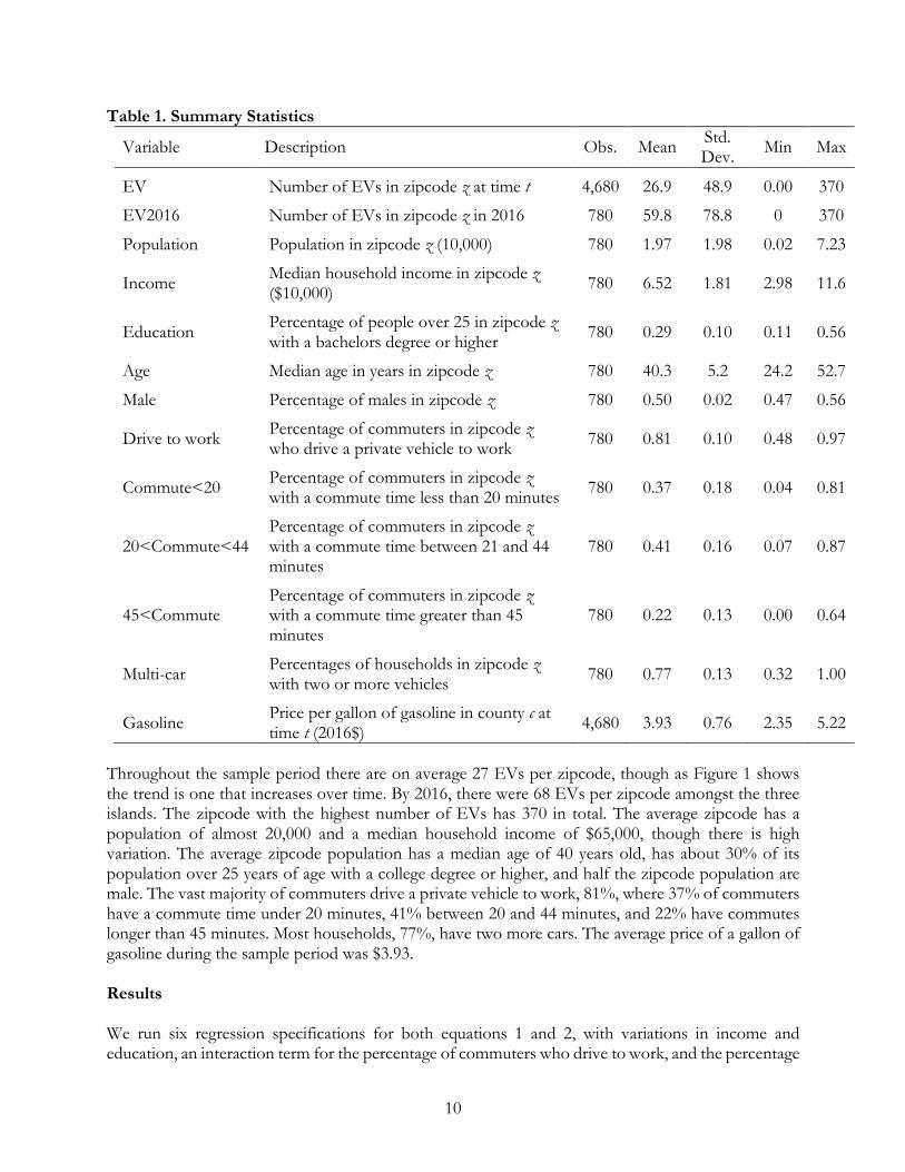
Table 1. Summary Statistics
Variable Description Obs. Mean Std. Dev. Min Max
EV Number of EVs in zipcode z at time t 4,680 26.9 48.9 0.00 370
EV2016 Number of EVs in zipcode z in 2016 780 59.8 78.8 0 370
Population Population in zipcode z (10,000) 780 1.97 1.98 0.02 7.23
Income Median household income in zipcode z ($10,000) 780 6.52 1.81 2.98 11.6
Education Percentage of people over 25 in zipcode z with a bachelors degree or higher 780 0.29 0.10 0.11 0.56
Age Median age in years in zipcode z 780 40.3 5.2 24.2 52.7
Male Percentage of males in zipcode z 780 0.50 0.02 0.47 0.56
Drive to work Percentage of commuters in zipcode z who drive a private vehicle to work 780 0.81 0.10 0.48 0.97
Commute<20 Percentage of commuters in zipcode z with a commute time less than 20 minutes 780 0.37 0.18 0.04 0.81
20<Commute<44 Percentage of commuters in zipcode z with a commute time between 21 and 44 minutes
780 0.41 0.16 0.07 0.87
45<Commute Percentage of commuters in zipcode z with a commute time greater than 45 minutes
780 0.22 0.13 0.00 0.64
Multi-car Percentages of households in zipcode z with two or more vehicles 780 0.77 0.13 0.32 1.00
Gasoline Price per gallon of gasoline in county c at time t (2016$) 4,680 3.93 0.76 2.35 5.22
Throughout the sample period there are on average 27 EVs per zipcode, though as Figure 1 shows the trend is one that increases over time. By 2016, there were 68 EVs per zipcode amongst the three islands. The zipcode with the highest number of EVs has 370 in total. The average zipcode has a population of almost 20,000 and a median household income of $65,000, though there is high variation. The average zipcode population has a median age of 40 years old, has about 30% of its population over 25 years of age with a college degree or higher, and half the zipcode population are male. The vast majority of commuters drive a private vehicle to work, 81%, where 37% of commuters have a commute time under 20 minutes, 41% between 20 and 44 minutes, and 22% have commutes longer than 45 minutes. Most households, 77%, have two more cars. The average price of a gallon of gasoline during the sample period was $3.93. Results We run six regression specifications for both equations 1 and 2, with variations in income and education, an interaction term for the percentage of commuters who drive to work, and the percentage

11
of households that have two or more vehicles. Specification 1 acts as our baseline, where we use income, an interaction term for the percentage of commuters that drive to work and exclude the variable for multi-car households. Specifications 2 and 3 are variations on dropping the relative variable for the bins related to commute time (i.e. dropping <20 minutes in comparison to >45 minutes). Relative to the baseline, specification 4 excludes income and adds education, and specification 5 adds in the variable for multi-car households. However, it is having multiple vehicles is highly correlated with driving to work. Specification 6 retains the variable for multi-car but omits the interaction with the percentage of commuters that drive to work and focuses solely on duration of commute.
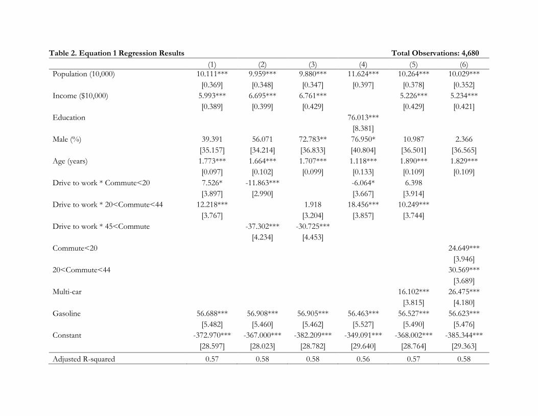
Table 2. Equation 1 Regression Results Total Observations: 4,680 (1) (2) (3) (4) (5) (6) Population (10,000) 10.111*** 9.959*** 9.880*** 11.624*** 10.264*** 10.029***
[0.369] [0.348] [0.347] [0.397] [0.378] [0.352] Income ($10,000) 5.993*** 6.695*** 6.761***
5.226*** 5.234***
[0.389] [0.399] [0.429]
[0.429] [0.421] Education
76.013***
[8.381]
Male (%) 39.391 56.071 72.783** 76.950* 10.987 2.366 [35.157] [34.214] [36.833] [40.804] [36.501] [36.565]
Age (years) 1.773*** 1.664*** 1.707*** 1.118*** 1.890*** 1.829*** [0.097] [0.102] [0.099] [0.133] [0.109] [0.109]
Drive to work * Commute<20 7.526* -11.863***
-6.064* 6.398
[3.897] [2.990]
[3.667] [3.914]
Drive to work * 20<Commute<44 12.218***
1.918 18.456*** 10.249***
[3.767]
[3.204] [3.857] [3.744]
Drive to work * 45<Commute
-37.302*** -30.725***
[4.234] [4.453]
Commute<20
24.649*** [3.946]
20<Commute<44
30.569*** [3.689]
Multi-car
16.102*** 26.475*** [3.815] [4.180]
Gasoline 56.688*** 56.908*** 56.905*** 56.463*** 56.527*** 56.623*** [5.482] [5.460] [5.462] [5.527] [5.490] [5.476]
Constant -372.970*** -367.000*** -382.209*** -349.091*** -368.002*** -385.344*** [28.597] [28.023] [28.782] [29.640] [28.764] [29.363]
Adjusted R-squared 0.57 0.58 0.58 0.56 0.57 0.58
13
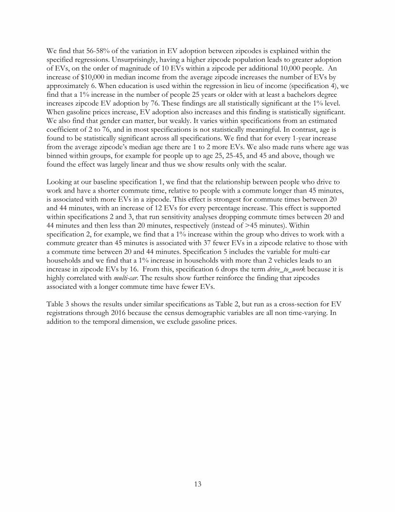
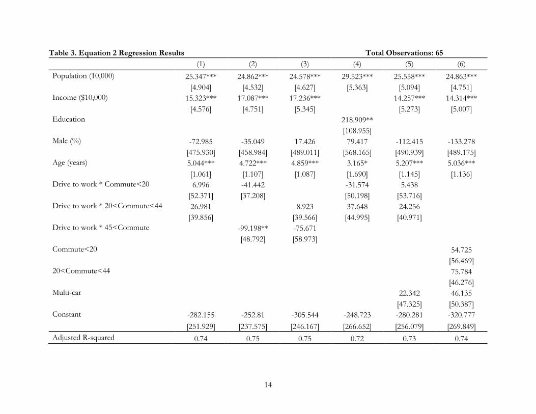
We find that 56-58% of the variation in EV adoption between zipcodes is explained within the specified regressions. Unsurprisingly, having a higher zipcode population leads to greater adoption of EVs, on the order of magnitude of 10 EVs within a zipcode per additional 10,000 people. An increase of $10,000 in median income from the average zipcode increases the number of EVs by approximately 6. When education is used within the regression in lieu of income (specification 4), we find that a 1% increase in the number of people 25 years or older with at least a bachelors degree increases zipcode EV adoption by 76. These findings are all statistically significant at the 1% level. When gasoline prices increase, EV adoption also increases and this finding is statistically significant. We also find that gender can matter, but weakly. It varies within specifications from an estimated coefficient of 2 to 76, and in most specifications is not statistically meaningful. In contrast, age is found to be statistically significant across all specifications. We find that for every 1-year increase from the average zipcode’s median age there are 1 to 2 more EVs. We also made runs where age was binned within groups, for example for people up to age 25, 25-45, and 45 and above, though we found the effect was largely linear and thus we show results only with the scalar. Looking at our baseline specification 1, we find that the relationship between people who drive to work and have a shorter commute time, relative to people with a commute longer than 45 minutes, is associated with more EVs in a zipcode. This effect is strongest for commute times between 20 and 44 minutes, with an increase of 12 EVs for every percentage increase. This effect is supported within specifications 2 and 3, that run sensitivity analyses dropping commute times between 20 and 44 minutes and then less than 20 minutes, respectively (instead of >45 minutes). Within specification 2, for example, we find that a 1% increase within the group who drives to work with a commute greater than 45 minutes is associated with 37 fewer EVs in a zipcode relative to those with a commute time between 20 and 44 minutes. Specification 5 includes the variable for multi-car households and we find that a 1% increase in households with more than 2 vehicles leads to an increase in zipcode EVs by 16. From this, specification 6 drops the term drive_to_work because it is highly correlated with multi-car. The results show further reinforce the finding that zipcodes associated with a longer commute time have fewer EVs. Table 3 shows the results under similar specifications as Table 2, but run as a cross-section for EV registrations through 2016 because the census demographic variables are all non time-varying. In addition to the temporal dimension, we exclude gasoline prices.
14
Table 3. Equation 2 Regression Results Total Observations: 65 (1) (2) (3) (4) (5) (6) Population (10,000) 25.347*** 24.862*** 24.578*** 29.523*** 25.558*** 24.863***
[4.904] [4.532] [4.627] [5.363] [5.094] [4.751] Income ($10,000) 15.323*** 17.087*** 17.236*** 14.257*** 14.314***
[4.576] [4.751] [5.345] [5.273] [5.007] Education 218.909**
[108.955] Male (%) -72.985 -35.049 17.426 79.417 -112.415 -133.278
[475.930] [458.984] [489.011] [568.165] [490.939] [489.175] Age (years) 5.044*** 4.722*** 4.859*** 3.165* 5.207*** 5.036***
[1.061] [1.107] [1.087] [1.690] [1.145] [1.136] Drive to work * Commute<20 6.996 -41.442 -31.574 5.438
[52.371] [37.208] [50.198] [53.716] Drive to work * 20<Commute<44 26.981 8.923 37.648 24.256
[39.856] [39.566] [44.995] [40.971] Drive to work * 45<Commute -99.198** -75.671
[48.792] [58.973] Commute<20 54.725
[56.469] 20<Commute<44 75.784
[46.276] Multi-car 22.342 46.135
[47.325] [50.387] Constant -282.155 -252.81 -305.544 -248.723 -280.281 -320.777 [251.929] [237.575] [246.167] [266.652] [256.079] [269.849] Adjusted R-squared 0.74 0.75 0.75 0.72 0.73 0.74
15
The results of Table 3 are quite similar to those presented in Table 2, in terms of sign and significance. However, we find that the magnitudes are appreciably larger in Table 3 for the estimated coefficients. This is due to the estimation being only for the last time frame where there is a greater number of EVs. The estimated coefficients for which there are other variations is for Male, where it is no longer statistically significant any in of the specifications. In addition, the finding that zipcodes associated with longer than 45 minute commute times are associated with fewer EVs is only statistically significant for specification 2 (although the directionality is similar in specification 3). In addition to the specifications shown in Table 2, we present additional sensitivity tests in Appendix II. The first uses a dependent variable measured as the number of new EVs each month within the zipcode, rather than the accumulation of EVs. The reason for this is because there is likely autocorrelation between dependent variables when shown as a cumulative number, as there are few EVs in many zipcodes. Because a number of zipcodes actually have zero EVs over the time period, particularly for Hawaii and Maui, we also present results for just Oahu. There are notable differences in results for Oahu only, particularly for the role of commute times, gasoline prices, and multi-car households. This is discussed within Appendix II. Future versions of this work will further delve into functional form, given the data limitations. Discussion & Conclusion Much of the literature forecasting EV adoption relies on survey estimates. This study provides an initial baseline of factors affecting EV purchase and registration decisions using empirical data for Hawaii. This study analyzes factors affecting EV adoption by leveraging differences in demographic data by zipcode and gasoline prices by island. We find that both income and education have a positive and statistically significant effect on EV adoption. There is some evidence that being gender and age are also related to additional EV adoption, where men are more likely to purchase an EV. We find interesting results in regard to the role of driving to work and commute times, where having a commute time over 45 minutes is associated with a decrease in EV adoption. This is likely related to what the literature refers to as “range anxiety,” even within an island context. We find that having two or more vehicles statewide is also associated with greater adoption of EVs, but this finding does not hold when looking at Oahu only (see Appendix II). Similarly, higher gasoline prices are associated with greater adoption of EVs statewide, though this relationship becomes negative when looking at Oahu only. This is likely because Oahu has a relatively higher dependence on oil for electricity generation. Integrating new vehicle technologies within the stock of over 1 million registered passenger vehicles (DBEDT, 2018) is by definition a relatively slow process, as approximately one in nine households in Hawaii expect to purchase a new car each year (HEPF, 2010). When considering the wide range of vehicle purchase decisions, EVs comprise a small, yet growing, share of new car purchases. Based on new vehicle registrations at the zipcode level from 2010 to 2016, the highest share of EVs is in zipcode 96821 on Oahu at 4.2% (see Appendix I). Though this analysis and results provide baseline information on early EV adoption, its policy implications are yet unclear. For example, commute times greater than 45 minutes are found to be negatively associated with EV adoption, raising potential implications for charging infrastructure and the network of necessary infrastructure to support additional EV driving distances. The provision of charging infrastructure is highly subjective to vehicle driving range, however, which is generally improving. In addition, charging time has been found to be critically important to consumers perceptions about willingness to purchase an EV

16
(Graham-Rowe et al., 2012), though consumer value for fast charging and driving range are inversely related (Dimitropoulous et al., 2013). Moreover, there must also be consideration for substitution between public charging stations and home charging (Ito et al., 2013). Thus, though we know that longer commute times are likely deterring EV adoption, there is still a need to conduct a more detailed study on public charging infrastructure in the context of improving vehicle characteristics and private access to charging.
17
References American Community Survey (2015a). Median Household Income in the Past 12 Months (in 2015 inflation-adjusted dollars). 2011 – 2015 American Community Survey 5-Year Estimates. B19013. American Community Survey. (2015b). Educational Attainment and Employment Status by Language Spoken at Home for the Population 25 Years and Over. 2011 – 2015 American Community Survey 5-Year Estimates. B16010. American Community Survey (2015c). Means of Transportation to Work. 2011 – 2015 American Community Survey 5-Year Estimates. B08301. American Community Survey (2015d). Means of Transportation to Work by Selected Characteristics. 2011 – 2015 American Community Survey 5-Year Estimates. S0802. Al-Alawi, B. and Bradley, T. (2013a). Total cost of ownership, payback, and consumer preference modeling of plug-in hybrid electric vehicles. Applied Energy, 103, 488-506. Axsen, J. and Kurani, K. (2011). Interpersonal influence in the early plug-in hybrid market: Observing social interactions with an exploratory multi-method approach. Transportation Research Part D, 16(2), 150-159.
Bakker, S., Maat, K., & Wee, B. (2014). Stakeholders interest, expectations, and strategies regarding the development and implementation of electric vehicles: The case of the Netherlands. Transportation Research Part A, 66, 52-64. Beresteanu, A. and Li, S. (2011). Gasoline prices, government support and the demand for hybrid vehicles in the United States. International Economic Review, 52(1), 161-182. Campbell, A., Ryley, T., & Thring, R. (2012). Identifying the early adopters of alternative fuel vehicles: A case study of Birmingham, United Kingdom. Transportation Research Part A: Policy and Practice, 46, 1318-1327. Carley, S., Krause, R., Lane, B., & Graham, J. (2013). Intent to purchase a plug-in electric vehicle: A survey of early impressions in large US cities. Transportation Research Part D, 18, 39-45. Coffman, M., Bernstein, P., & Wee, S. (2016a). Integrating Electric Vehicles and Residential Solar PV. Transport Policy, 53, 30-38. Coffman, M., Bernstein, P., & Wee, S. (2016b). Electric Vehicles Revisited: A Review of Factors that Affect Adoption. Transport Reviews, 37(1), 79-93. Department of Business Economic Development and Tourism (DBEDT) (2018). Data Warehouse, Registered Vehicles, Taxable Passenger and Electric, Passenger. Reported monthly through December 2017. Available at: http://dbedt.hawaii.gov/economic/datawarehouse/
18
Department of Business, Economic Development, and Tourism (DBEDT) (2017). Data Warehouse, Gasoline price-regular and Electricity Retail Prices (Average price per kWh) - residential. Reported monthly through December 2016. Available at: http://dbedt.hawaii.gov/economic/datawarehouse/ Department of Transportation (DOT) (2017). DMV Registration Dataset. Vehicles registered as of 14 February 2017. State of Hawaii. Diamond, D. (2009). The impact of government incentives for hybrid-electric vehicles: Evidence from US states. Energy Policy, 37, 972-983. Dimitropoulos, A., Rietveld, P., & Ommeren, J. (2013). Consumer valuation of changes in driving range: A meta-analysis. Transportation Research Part A, 55, 27-45. Egbue, O. and Long, S. (2012). Barriers to widespread adoption of electric vehicles: An analysis of consumer attitudes and perceptions. Energy Policy, 48, 717-729. Gallagher, K. and Muehlegger, E. (2011). Giving green to get green? Incentives and consumer adoption of hybrid vehicle technology. Journal of Environmental Economics and Management, 61(1), 1-15. Giambelluca, T.W., X. Shuai, M.L. Barnes, R.J. Alliss, R.J. Longman, T. Miura, Q. Chen, A.G. Frazier, R.G. Mudd, L. Cuo, and A.D. Businger. (2014). Evapotranspiration of Hawai‘i. Final report submitted to the U.S. Army Corps of Engineers—Honolulu District, and the Commission on Water Resource Management, State of Hawai‘i. Graham-Rowe, E., Gardner, B., Abraham, C., Skippon, S., Dittmar, H., Hutchins, R., & Stannard, J. (2012). Mainstream consumers driving plug-in battery-electric and plug-in hybrid electric cars: A qualitative analysis of responses and evaluations. Transportation Research Part A, 46, 140-153. Hackbarth, A. and Madlener, R. (2013). Consumer preferences for alternative fuel vehicles: A discrete choice analysis. Transportation Research Part D, 25, 5-17. Hawaiian Electric Companies. (2017). 2016 Renewable Portfolio Standard Status Report. Docket No. 2007-0008. Available at: https://puc.hawaii.gov/wp-content/uploads/2013/07/RPS-HECO-2016.pdf Hawkins, T., Gausen, O., and Strømman, A. (2012). Environmental impacts of hybrid and electric vehicles—a review. International Journal of Life Cycle Assessment, 17, 997-1014. Hawaii Energy Policy Forum (HEPF) (2010). Final Report. Strategies for Energy Efficiencies in Transportation. Available at: http://www.hawaiienergypolicy.hawaii.edu/programs-initiatives/transportation-options-efficiency/_downloads/wg-t-report-statewide.pdf
Hidrue, M., Parsons, G., Kempton, W., & Gardner, M. (2011). Willingness to Pay for Electric Vehicles and their Attributes. Resource and Energy Economics, 33, 686-705.
19
Ito, N., Takeuchi, K., & Managi, S. (2013). Willingness to pay for infrastructure investments for alternative fuel vehicles. Transportation Research Part D, 18, 1-8.
Jensen, A., Cherchi, E., & Mabit, S. (2013). On the stability of preferences and attitudes before and after experiencing an electric vehicle. Transportation Research, 25, 24-32.
Lincoln, M. (2013). Electric Vehicles Charging Station Law Lacks Enforcement. Hawaii News Now. Available at: http://www.hawaiinewsnow.com/story/23098457/electric-vehicle-charging-station-law-lacks-enforcement Lopes, M., Moura, F., & Martinez, L. (2014). A rule-based approach for determining the plausible universe of electric vehicle buyers in the Lisbon metropolitan area. Transportation Research Part A, 59, 22-44. Lutsey, N. (2015). Global milestone: The first million electric vehicles. The International Council on Clean Transportation (ICCT). Blog Post. Retrieved from https://www.theicct.org/blog/staff/global-milestone-first-million-electric-vehicles Onat, N., Kucukvar, M., & Tatari, O. (2015). Conventional, hybrid, plug-in hybrid or electric vehicles? State-based comparatie carbon and energy footprint analysis in the United States. Applied Energy, 150, 36-49. Prud’homme, R., and Koning, M. (2012). Electric vehicles: A tentative economic and environmental evaluation. Transport Policy, 23, 60-69. Samaras, C. and Meisterling, K. (2008). Life Cycle Assessment of Greenhouse Gas Emissions from Plug-In Hybrid Vehicles: Implications for Policy. Environmental Science & Technology, 42(9), 3170-3176. Schroeder, A., and Traber, T. (2012). The economics of fast charging infrastructure for electric vehicles. Energy Policy, 43, 136-144. Stephen, C. and Sullivan, J. (2008). Environmental and Energy Implications of Plug-In Hybrid-Electric Vehicles. Environmental Science & Technology, 42(4), 1185-1190. Sierzchula, W., Bakker, S., Maat, K., & Wee, B. (2014). The influence of financial incentives and other socio-economic factors on electric vehicle adoption. Energy Policy, 68, 183-194. Tran, M., Banister, D., Bishop, J., & McCullogh, M. (2013). Simulating early adoption of alternative fuel vehicles for sustainability. Technological Forecasting & Social Change, 80, 865-875.
Tseng, H., Wu, J., & Liu, X. (2013). Affordability of electric vehicles for a sustainable transport system: An economic and environmental analysis. Energy Policy, 61, 441-447. Tuttle, B. (2015). “So About That Goal of 1 Million Electric Cars by 2015…” Available at: http://time.com/money/3677021/obama-electric-cars-gas/

20
U.S. Census Bureau (2010). Profile of General Population and Housing Characteristics: 2010. 2010 Demographic Profile Data. DP-1. U.S. Bureau of Labor Statistics (BLS). (2017). Honolulu Consumer Price Index. Accessed 4 March 2017. U.S. Department of Labor. Available at: http://data.bls.gov/pdq/SurveyOutputServlet?series_id=CUURA426SA0,CUUSA426SA0 U.S. Energy Information Administration (EIA). (2017). EIA-923 Monthly Generation and Fuel Consumption Time Series File, 2016 Final Revision. Available at: https://www.eia.gov/electricity/data/eia923/ Wu, X., Dong, J., & Lin, Z. (2014). Cost analysis of plug-in electric vehicles using GPS-based longitudinal travel data. Energy Policy, 68, 206-217.
21
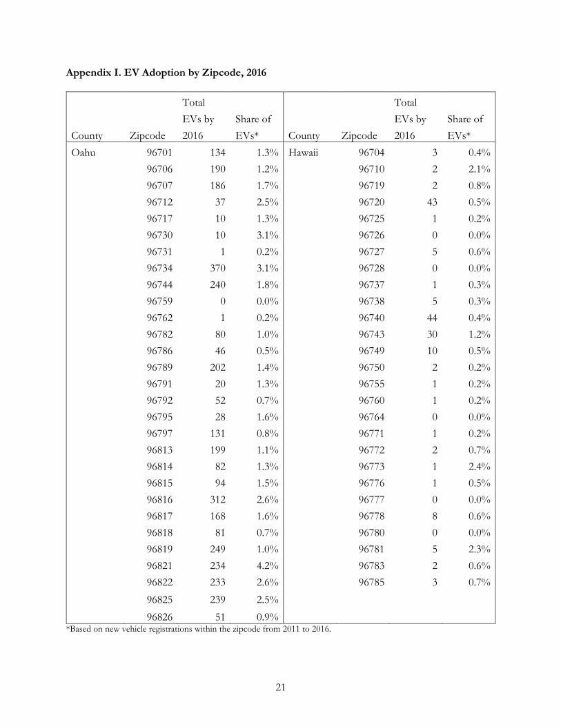
Appendix I. EV Adoption by Zipcode, 2016
County Zipcode
Total EVs by 2016
Share of EVs* County Zipcode
Total EVs by 2016
Share of EVs*
Oahu 96701 134 1.3% Hawaii 96704 3 0.4% 96706 190 1.2% 96710 2 2.1% 96707 186 1.7% 96719 2 0.8% 96712 37 2.5% 96720 43 0.5% 96717 10 1.3% 96725 1 0.2% 96730 10 3.1% 96726 0 0.0% 96731 1 0.2% 96727 5 0.6% 96734 370 3.1% 96728 0 0.0% 96744 240 1.8% 96737 1 0.3% 96759 0 0.0% 96738 5 0.3% 96762 1 0.2% 96740 44 0.4% 96782 80 1.0% 96743 30 1.2% 96786 46 0.5% 96749 10 0.5% 96789 202 1.4% 96750 2 0.2% 96791 20 1.3% 96755 1 0.2% 96792 52 0.7% 96760 1 0.2% 96795 28 1.6% 96764 0 0.0% 96797 131 0.8% 96771 1 0.2% 96813 199 1.1% 96772 2 0.7% 96814 82 1.3% 96773 1 2.4% 96815 94 1.5% 96776 1 0.5% 96816 312 2.6% 96777 0 0.0% 96817 168 1.6% 96778 8 0.6% 96818 81 0.7% 96780 0 0.0% 96819 249 1.0% 96781 5 2.3% 96821 234 4.2% 96783 2 0.6% 96822 233 2.6% 96785 3 0.7%
96825 239 2.5%
96826 51 0.9% *Based on new vehicle registrations within the zipcode from 2011 to 2016.
22
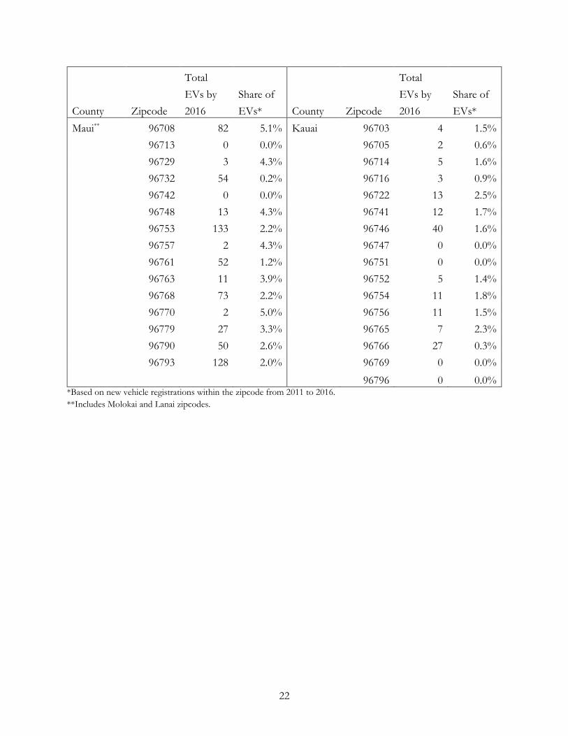
County Zipcode
Total EVs by 2016
Share of EVs* County Zipcode
Total EVs by 2016
Share of EVs*
Maui** 96708 82 5.1% Kauai 96703 4 1.5% 96713 0 0.0% 96705 2 0.6% 96729 3 4.3% 96714 5 1.6% 96732 54 0.2% 96716 3 0.9% 96742 0 0.0% 96722 13 2.5% 96748 13 4.3% 96741 12 1.7% 96753 133 2.2% 96746 40 1.6% 96757 2 4.3% 96747 0 0.0% 96761 52 1.2% 96751 0 0.0% 96763 11 3.9% 96752 5 1.4% 96768 73 2.2% 96754 11 1.8% 96770 2 5.0% 96756 11 1.5% 96779 27 3.3% 96765 7 2.3% 96790 50 2.6% 96766 27 0.3% 96793 128 2.0% 96769 0 0.0%
96796 0 0.0% *Based on new vehicle registrations within the zipcode from 2011 to 2016. **Includes Molokai and Lanai zipcodes.

23
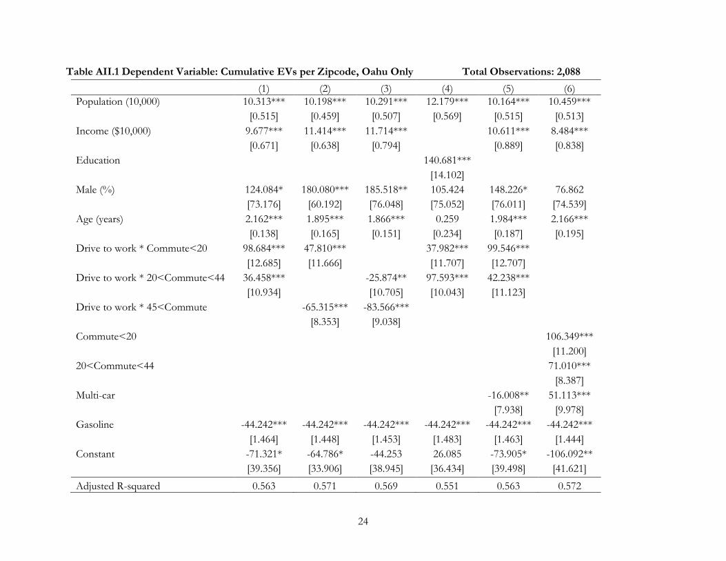
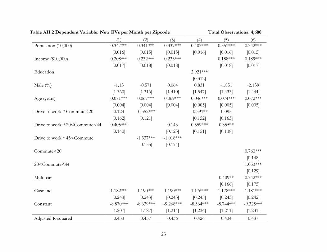
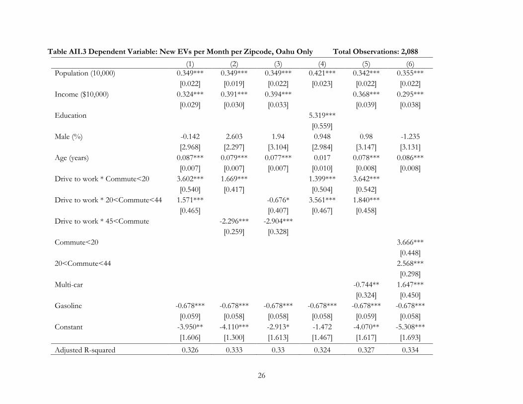
Appendix II. Additional Results from Sensitivity Analysis The following three tables contain results from sensitivity analysis where 1) we redefined the dependent variable as new EVs in a zipcode each month and 2) we look at Oahu only, as it is the island with the most EVs in total and between zipcodes. Table AII.1 shows the results for Oahu only where the dependent variable is still measured as the cumulative number of EVs in the zipcode in a month, comparable to Table 2. Table AII.2 shows the full sample estimated with the dependent variable as the number of new EVs only, and Table AII.3 looks at this alternative measure of the dependent variable for Oahu only. Oahu has a total of 29 zipcodes.
24
Table AII.1 Dependent Variable: Cumulative EVs per Zipcode, Oahu Only Total Observations: 2,088 (1) (2) (3) (4) (5) (6) Population (10,000) 10.313*** 10.198*** 10.291*** 12.179*** 10.164*** 10.459***
[0.515] [0.459] [0.507] [0.569] [0.515] [0.513] Income ($10,000) 9.677*** 11.414*** 11.714***
10.611*** 8.484***
[0.671] [0.638] [0.794]
[0.889] [0.838] Education
140.681***
[14.102]
Male (%) 124.084* 180.080*** 185.518** 105.424 148.226* 76.862 [73.176] [60.192] [76.048] [75.052] [76.011] [74.539]
Age (years) 2.162*** 1.895*** 1.866*** 0.259 1.984*** 2.166*** [0.138] [0.165] [0.151] [0.234] [0.187] [0.195]
Drive to work * Commute<20 98.684*** 47.810***
37.982*** 99.546***
[12.685] [11.666]
[11.707] [12.707]
Drive to work * 20<Commute<44 36.458***
-25.874** 97.593*** 42.238***
[10.934]
[10.705] [10.043] [11.123]
Drive to work * 45<Commute
-65.315*** -83.566***
[8.353] [9.038]
Commute<20
106.349*** [11.200]
20<Commute<44
71.010*** [8.387]
Multi-car
-16.008** 51.113*** [7.938] [9.978]
Gasoline -44.242*** -44.242*** -44.242*** -44.242*** -44.242*** -44.242*** [1.464] [1.448] [1.453] [1.483] [1.463] [1.444]
Constant -71.321* -64.786* -44.253 26.085 -73.905* -106.092** [39.356] [33.906] [38.945] [36.434] [39.498] [41.621]
Adjusted R-squared 0.563 0.571 0.569 0.551 0.563 0.572
25
Table AII.2 Dependent Variable: New EVs per Month per Zipcode Total Observations: 4,680 (1) (2) (3) (4) (5) (6) Population (10,000) 0.347*** 0.341*** 0.337*** 0.403*** 0.351*** 0.342***
[0.016] [0.015] [0.015] [0.016] [0.016] [0.015] Income ($10,000) 0.208*** 0.232*** 0.233***
0.188*** 0.189***
[0.017] [0.018] [0.018]
[0.018] [0.017] Education
2.921***
[0.312]
Male (%) -1.13 -0.571 0.064 0.831 -1.851 -2.139 [1.360] [1.316] [1.410] [1.547] [1.433] [1.444]
Age (years) 0.071*** 0.067*** 0.069*** 0.046*** 0.074*** 0.072*** [0.004] [0.004] [0.004] [0.005] [0.005] [0.005]
Drive to work * Commute<20 0.124 -0.552***
-0.391** 0.095
[0.162] [0.121]
[0.152] [0.163]
Drive to work * 20<Commute<44 0.405***
0.143 0.559*** 0.355**
[0.140]
[0.123] [0.151] [0.138]
Drive to work * 45<Commute
-1.337*** -1.018***
[0.155] [0.174]
Commute<20
0.763*** [0.148]
20<Commute<44
1.053*** [0.129]
Multi-car
0.409** 0.742*** [0.166] [0.175]
Gasoline 1.182*** 1.190*** 1.190*** 1.176*** 1.178*** 1.181*** [0.243] [0.243] [0.243] [0.245] [0.243] [0.242]
Constant -8.870*** -8.639*** -9.268*** -8.364*** -8.744*** -9.325*** [1.207] [1.187] [1.214] [1.236] [1.211] [1.231]
Adjusted R-squared 0.433 0.437 0.436 0.426 0.434 0.437
26
Table AII.3 Dependent Variable: New EVs per Month per Zipcode, Oahu Only Total Observations: 2,088 (1) (2) (3) (4) (5) (6) Population (10,000) 0.349*** 0.349*** 0.349*** 0.421*** 0.342*** 0.355***
[0.022] [0.019] [0.022] [0.023] [0.022] [0.022] Income ($10,000) 0.324*** 0.391*** 0.394***
0.368*** 0.295***
[0.029] [0.030] [0.033]
[0.039] [0.038] Education
5.319***
[0.559]
Male (%) -0.142 2.603 1.94 0.948 0.98 -1.235 [2.968] [2.297] [3.104] [2.984] [3.147] [3.131]
Age (years) 0.087*** 0.079*** 0.077*** 0.017 0.078*** 0.086*** [0.007] [0.007] [0.007] [0.010] [0.008] [0.008]
Drive to work * Commute<20 3.602*** 1.669***
1.399*** 3.642***
[0.540] [0.417]
[0.504] [0.542]
Drive to work * 20<Commute<44 1.571***
-0.676* 3.561*** 1.840***
[0.465]
[0.407] [0.467] [0.458]
Drive to work * 45<Commute
-2.296*** -2.904***
[0.259] [0.328]
Commute<20
3.666*** [0.448]
20<Commute<44
2.568*** [0.298]
Multi-car
-0.744** 1.647*** [0.324] [0.450]
Gasoline -0.678*** -0.678*** -0.678*** -0.678*** -0.678*** -0.678*** [0.059] [0.058] [0.058] [0.058] [0.059] [0.058]
Constant -3.950** -4.110*** -2.913* -1.472 -4.070** -5.308*** [1.606] [1.300] [1.613] [1.467] [1.617] [1.693]
Adjusted R-squared 0.326 0.333 0.33 0.324 0.327 0.334
27
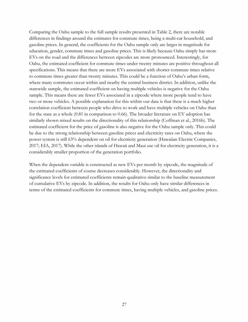
Comparing the Oahu sample to the full sample results presented in Table 2, there are notable differences in findings around the estimates for commute times, being a multi-car household, and gasoline prices. In general, the coefficients for the Oahu sample only are larger in magnitude for education, gender, commute times and gasoline prices. This is likely because Oahu simply has more EVs on the road and the differences between zipcodes are more pronounced. Interestingly, for Oahu, the estimated coefficient for commute times under twenty minutes are positive throughout all specifications. This means that there are more EVs associated with shorter commute times relative to commute times greater than twenty minutes. This could be a function of Oahu’s urban form, where many commutes occur within and nearby the central business district. In addition, unlike the statewide sample, the estimated coefficient on having multiple vehicles is negative for the Oahu sample. This means there are fewer EVs associated in a zipcode where more people tend to have two or more vehicles. A possible explanation for this within our data is that there is a much higher correlation coefficient between people who drive to work and have multiple vehicles on Oahu than for the state as a whole (0.81 in comparison to 0.66). The broader literature on EV adoption has similarly shown mixed results on the directionality of this relationship (Coffman et al., 2016b). The estimated coefficient for the price of gasoline is also negative for the Oahu sample only. This could be due to the strong relationship between gasoline prices and electricity rates on Oahu, where the power system is still 63% dependent on oil for electricity generation (Hawaiian Electric Companies, 2017; EIA, 2017). While the other islands of Hawaii and Maui use oil for electricity generation, it is a considerably smaller proportion of the generation portfolio. When the dependent variable is constructed as new EVs per month by zipcode, the magnitude of the estimated coefficients of course decreases considerably. However, the directionality and significance levels for estimated coefficients remain qualitative similar to the baseline measurement of cumulative EVs by zipcode. In addition, the results for Oahu only have similar differences in terms of the estimated coefficients for commute times, having multiple vehicles, and gasoline prices.
28
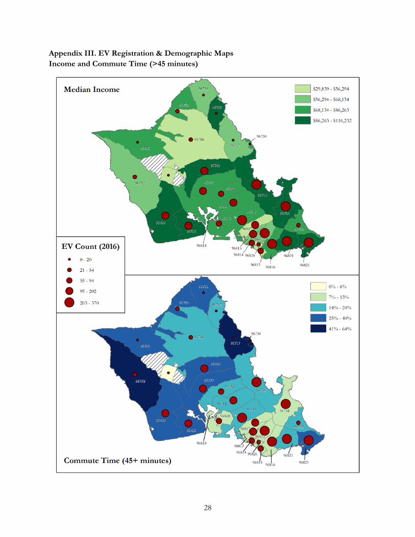
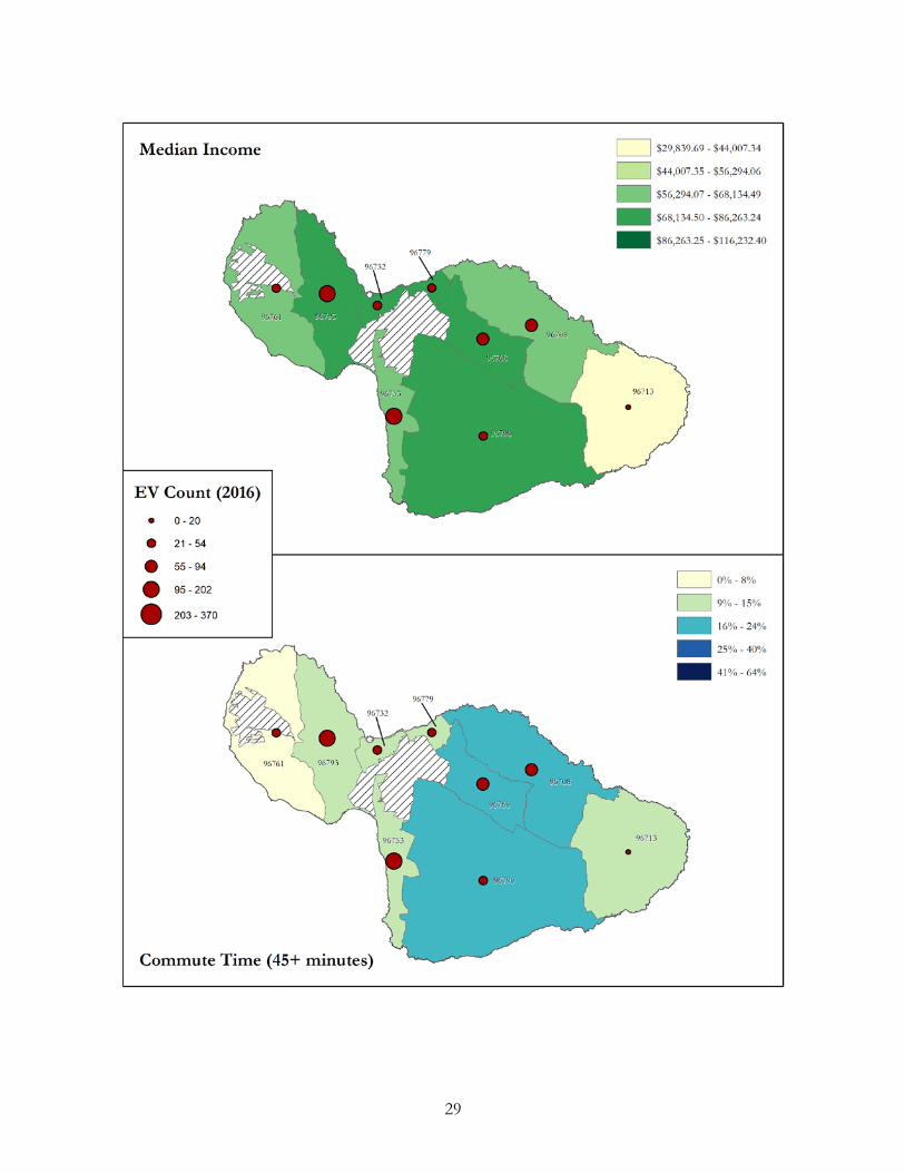
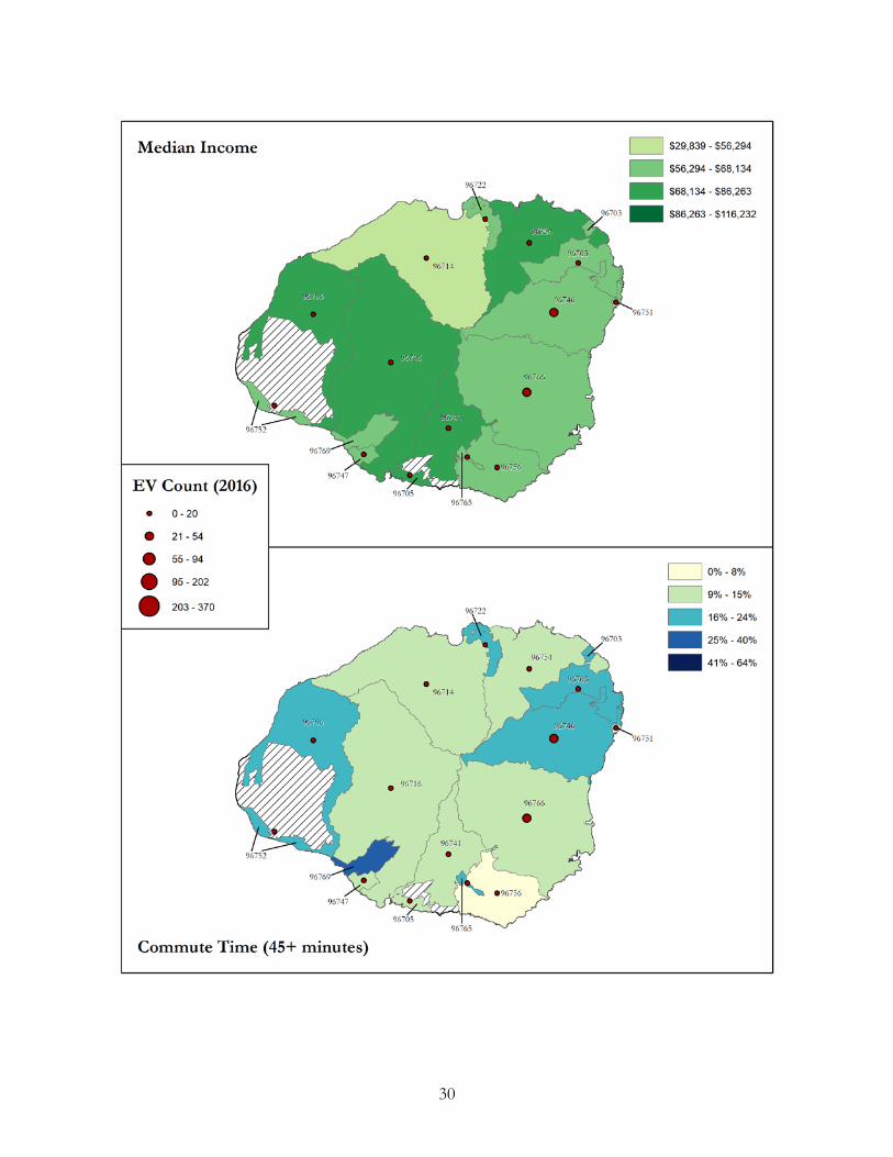
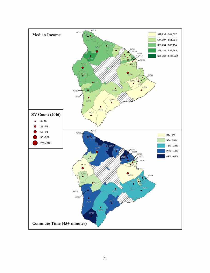
Appendix III. EV Registration & Demographic Maps Income and Commute Time (>45 minutes)
29
30
31