Embed Size (px)
Citation preview

What Measure of Inflation Should a Central Bank Target?
N. Gregory Mankiw
Harvard University
Ricardo Reis1
Harvard University
December 2002
1We are grateful to Ignazio Angeloni, William Dupor, Stanley Fischer, Yves Nosbusch, the editorRoberto Perotti, and anonymous referees for helpful comments. Reis is grateful to the FundacaoCiencia e Tecnologia, Praxis XXI, for financial support.

Abstract
This paper assumes that a central bank commits itself to maintaining an inflation target
and then asks what measure of the inflation rate the central bank should use if it wants
to maximize economic stability. The paper first formalizes this problem and examines its
microeconomic foundations. It then shows how the weight of a sector in the stability price
index depends on the sector’s characteristics, including size, cyclical sensitivity, sluggishness
of price adjustment, and magnitude of sectoral shocks. When a numerical illustration of
the problem is calibrated to U.S. data, one tentative conclusion is that a central bank that
wants to achieve maximum stability of economic activity should use a price index that gives
substantial weight to the level of nominal wages.

Over the past decade, many central banks around the world have adopted inflation tar-
geting as a guide for the conduct of monetary policy. In such a regime, the price level
becomes the economy’s nominal anchor, much as a monetary aggregate would be under a
monetarist policy rule. Inflation targeting is often viewed as a way to prevent the wild
swings in monetary policy that were responsible for, or at least complicit in, many of the
macroeconomic mistakes of the past. A central bank committed to inflation targeting would
likely have avoided both the big deflation during the Great Depression of the 1930s and the
accelerating inflation of the 1970s (and thus the deep disinflationary recession that followed).
This paper takes as its starting point that a central bank has adopted a regime of inflation
targeting and asks what measure of the inflation rate it should target. Our question might
at first strike some readers as odd. Measures of the overall price level, such as the consumer
price index, are widely available and have been amply studied by index-number theorists.
Yet a price index designed to measure the cost of living is not necessarily the best one to
serve as a target for a monetary authority.
This issue is often implicit in discussions of monetary policy. Many economists pay close
attention to “core inflation,” defined as inflation excluding certain volatile prices, such as
food and energy prices. Others suggest that commodity prices might be particularly good
indicators because they are highly responsive to changing economic conditions. Similarly,
during the U.S. stock market boom of the 1990s, some economists called for Fed tightening
to dampen “asset price inflation,” suggesting that the right index for monetary policy might
include not only the prices of goods and services but asset prices as well. Various monetary
proposals can be viewed as inflation targeting with a nonstandard price index: The gold
standard uses only the price of gold, and a fixed exchange rate uses only the price of a
foreign currency.
In this paper, we propose and explore an approach to choosing a price index for the
central bank to target. We are interested in finding the price index that, if kept on an
assigned target, would lead to the greatest stability in economic activity. This concept
might be called the stability price index.
The key issue in the construction of any price index is the weights assigned to the prices
from different sectors of the economy. When constructing a price index to measure the cost
1

of living, the natural weights are the share of each good in the budget of typical consumer.
When constructing a price index for the monetary authority to target, additional concerns
come into play: the cyclical sensitivity of each sector, the proclivity of each sector to expe-
rience idiosyncratic shocks, and the speed with which the prices in each sector respond to
changing conditions.
Our goal in this paper is to show how the weights in a stability price index should
depend on these sectoral characteristics. Section 1 sets up the problem. Section 2 examines
the microeconomic foundations for the problem set forth in Section 1. Section 3 presents and
discusses the analytic solution for the special case with only two sectors. Section 4 presents
a more realistic numerical illustration, which we calibrate with plausible parameter values
for the U.S. economy. One tentative conclusion is that the stability price index should give
a substantial weight to the level of nominal wages.
1 The Optimal Price Index: Statement of the Problem
Here we develop a framework to examine the optimal choice of a price index. To keep things
simple, the model includes only a single period of time. The central bank is committed to
inflation targeting in the following sense: Before the shocks are realized, the central bank
must choose a price index and commit itself to keeping that index on target.
The model includes many sectoral prices, which differ according to four characteristics.
(1) Sectors differ in their budget share and thus the weight their prices receive in a standard
price index. (2) In some sectors equilibrium prices are highly sensitive to the business cycle,
while in other sectors equilibrium prices are less cyclical. (3) Some sectors experience large
idiosyncratic shocks, while other sectors do not. (4) Some prices are flexible, while others
are sluggish in responding to changing economic conditions.
To formalize these sectoral differences, we borrow from the so-called “new Keynesian”
literature on price adjustment. We begin with an equation for the equilibrium price in sector
k:
p∗k = p+ αkx+ εk (1)
2

where, with all variables expressed in logs, p∗k is the equilibrium price in sector k, p is the
price level as conventionally measured (such as the CPI), αk is the sensitivity of sector k’s
equilibrium price to the business cycle, x is the output gap (the deviation of output from its
natural level), and εk is an idiosyncratic shock to sector k with variance σ2k. This equation
says only that the equilibrium relative price in a sector depends on the state of the business
cycle and some other shock. Sectors can differ in their sensitivities to the cycle and in the
variances of their idiosyncratic shocks.
In Section 2 we examine some possible microeconomic foundations for this model, but
readers may be familiar with the equation for the equilibrium price from the literature on
price setting under monopolistic competition.1 The index p represents the nominal variable
that shifts both demand and costs, and thus the equilibrium prices, in all the sectors. This
variable corresponds to a standard price index such as the CPI. That is, if there are K
sectors,
p =
KXk=1
θkpk
where θk are the weights of different sectors in the typical consumer’s budget. The output
gap x affects the equilibrium price by its influence on marginal cost and on the pricing
power of firms. One interpretation of the shocks εk is that they represent sectoral shocks
to productivity. In addition, they include changes in the degree of competition in sector k.
The formation of an oil cartel, for instance, would be represented by a positive value of εk
in the oil sector.
Sectors may also have sluggish prices. We model the sluggish adjustment by assuming
that some fraction of prices in a sector are predetermined. One rationale for this approach,
following Fischer (1977), is that some prices are set in advance by nominal contracts. An
alternative rationale, following Mankiw and Reis (2001a), is that price setters are slow to
update their plans because there are costs to acquiring or processing information. In either
case, the key feature for the purpose at hand is that some prices in the economy are set
based on old information and do not respond immediately to changing circumstances.
1For a textbook treatment, see Romer (2001, equation 6.45).
3

Let λk be the fraction of the price setters in sector k that set their prices based on updated
information, while 1− λk set prices based on old plans and outdated information. Thus, the
price in period t is determined by
pk = λkp∗k + (1− λk)E(p
∗k). (2)
The parameter λk measures how sluggish prices are in sector k. The smaller is λk, the less
responsive actual prices are to news about equilibrium prices. As λk approaches one, the
sector approaches the classical benchmark where actual and equilibrium prices are always
the same.
The central bank is assumed to be committed to targeting inflation. That is, the central
bank will keep a weighted average of sectoral prices at a given level, which we can set equal
to zero without loss of generality. We can write this as
KXk=1
ωkpk = 0 (3)
for some set of weights such that
KXk=1
ωk = 1.
We will call {ωk} the target weights and {θk} the consumption weights. The target weights
are choice variables of the central bank. The sectoral characteristics (θk, αk, λk, and σ2k) are
taken as exogenous.
We assume that the central bank dislikes volatility in economic activity. That is, its goal
is to minimize V ar(x). We abstract from the problem of monetary control by assuming that
the central bank can hit precisely whatever nominal target it chooses. The central question
of this paper is the choice of weights {ωk} that will lead to greatest macroeconomic stability.
Putting everything together, the central bank’s problem can now be stated as follows:
min{ωk}
V ar(x)
4
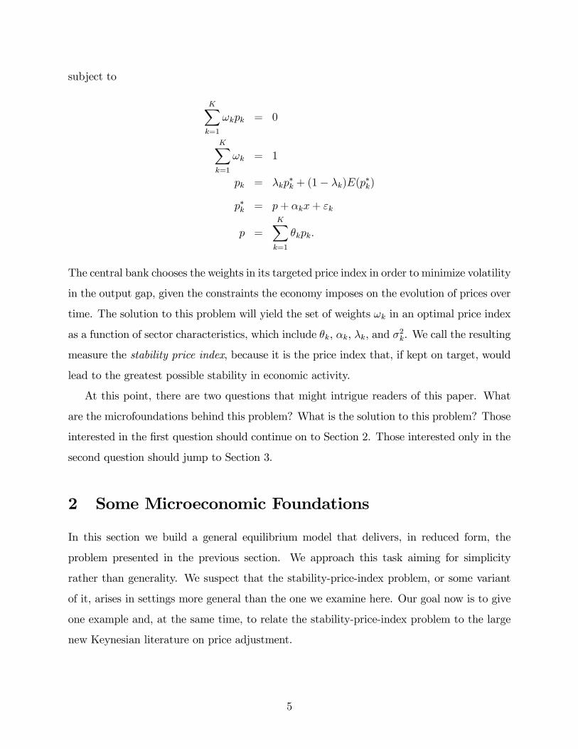
subject to
KXk=1
ωkpk = 0
KXk=1
ωk = 1
pk = λkp∗k + (1− λk)E(p
∗k)
p∗k = p+ αkx+ εk
p =KXk=1
θkpk.
The central bank chooses the weights in its targeted price index in order to minimize volatility
in the output gap, given the constraints the economy imposes on the evolution of prices over
time. The solution to this problem will yield the set of weights ωk in an optimal price index
as a function of sector characteristics, which include θk, αk, λk, and σ2k. We call the resulting
measure the stability price index, because it is the price index that, if kept on target, would
lead to the greatest possible stability in economic activity.
At this point, there are two questions that might intrigue readers of this paper. What
are the microfoundations behind this problem? What is the solution to this problem? Those
interested in the first question should continue on to Section 2. Those interested only in the
second question should jump to Section 3.
2 Some Microeconomic Foundations
In this section we build a general equilibrium model that delivers, in reduced form, the
problem presented in the previous section. We approach this task aiming for simplicity
rather than generality. We suspect that the stability-price-index problem, or some variant
of it, arises in settings more general than the one we examine here. Our goal now is to give
one example and, at the same time, to relate the stability-price-index problem to the large
new Keynesian literature on price adjustment.
5

2.1 The Economy Without Nominal Rigidities
The economy is populated by a continuum of yeoman farmers, indexed by their sector k and
by i within this sector. They derive utility from consumption C and disutility from labor
Lki, according to the common utility function:
U(C,Lki) =C1−σ
1− σ− Lki.
There are many types of consumption goods. Following Spence (1976) and Dixit and Stiglitz
(1977), we model the household’s demand for these goods using a constant elasticity of
substitution (CES) aggregate. Final consumption C is a CES aggregate over the goods in
the K sectors of the economy:
C =
"KXk=1
θ1γ
k Cγ−1γ
k
# γγ−1
. (4)
The parameter γ measures the elasticity of substitution across the K sectors. The weights
θk sum to one and express the relative size of each sector.
Within each sector, there are many farmers, represented by a continuum over the unit
interval. The sector’s output is also a CES aggregate of the farmers’ outputs:
Ck =
·Z 1
0
Cγ−1γ
ki di
¸ γγ−1. (5)
Notice that, for simplicity, we have assumed that the elasticity of substitution is the same
across sectors and across firms within a sector.2
Each farmer uses his labor to operate a production function, which takes the simple form:
Yki =¡e−ak(1 + ψ)Lki
¢1/(1+ψ). (6)
2As is usual, there are two ways to interpret these CES aggregators. The more common approach is toview them as representing consumers’ taste for variety. Alternatively, one can view C as the single final goodthat consumers buy and the CES aggregators as representing production functions for producing that finalgood from intermediate goods.
6
The ak stand for random productivity shock and ψ is a parameter that determines the degree
of returns to scale in production.
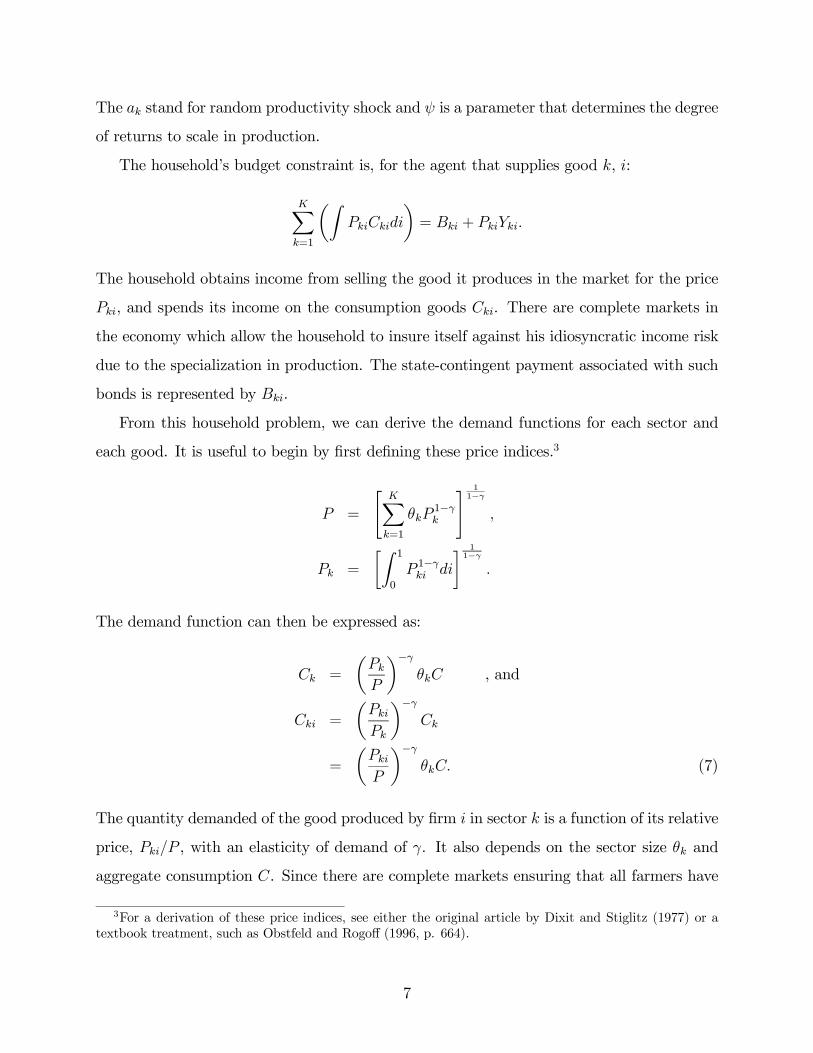
The household’s budget constraint is, for the agent that supplies good k, i:
KXk=1
µZPkiCkidi
¶= Bki + PkiYki.
The household obtains income from selling the good it produces in the market for the price
Pki, and spends its income on the consumption goods Cki. There are complete markets in
the economy which allow the household to insure itself against his idiosyncratic income risk
due to the specialization in production. The state-contingent payment associated with such
bonds is represented by Bki.
From this household problem, we can derive the demand functions for each sector and
each good. It is useful to begin by first defining these price indices.3
P =
"KXk=1
θkP1−γk
# 11−γ
,
Pk =
·Z 1
0
P 1−γki di
¸ 11−γ.
The demand function can then be expressed as:
Ck =
µPkP
¶−γθkC , and
Cki =
µPkiPk
¶−γCk
=
µPkiP
¶−γθkC. (7)
The quantity demanded of the good produced by firm i in sector k is a function of its relative
price, Pki/P , with an elasticity of demand of γ. It also depends on the sector size θk and
aggregate consumption C. Since there are complete markets ensuring that all farmers have
3For a derivation of these price indices, see either the original article by Dixit and Stiglitz (1977) or atextbook treatment, such as Obstfeld and Rogoff (1996, p. 664).
7

the same disposable income and they have the same preferences, they will all choose the
same level of consumption C.
Let’s now turn to the supply side of the goods market. The real marginal cost of pro-
ducing one unit of a good for every farmer equals the marginal rate of substitution between
consumption and leisure (the shadow cost of labor supply) divided by the marginal product
of labor:
MC(Yki) = CσeakY ψ
ki . (8)
We write the desired price of farmer i in sector k as:
P ∗kiP= mkMC(Yki). (9)
The relative price of any good is a markup mk times the real marginal cost of producing
the good. The markup mk can capture many possible market structures from standard
monopoly (which here implies mk = γ/(γ − 1)) to competition (mk = 1). We allow mk to
be both stochastic and a function of the level of economic activity.4 We express this as
mk = Yφkeµk
where µk is a random variable capturing shocks to the markup. The parameter φk governs
the cyclical sensitivity of the markups in sector k, and it can be either positive or negative.
We can now solve for the economy’s equilibrium. Using the pricing equation (9), the
demand function for variety i in sector k (7), and the market-clearing conditions that Cki =
Yki and C = Y , we obtain the following equation for the log of the equilibrium price:5
p∗k = p+ αky +µk + ak + ψ log(θk)
1 + γψ, (10)
4Rotemberg and Woodford (1999) survey alternative theories of why markups may vary over the businesscycle. Clarida, Gali and Gertler (2002) and Steinsson (2002) consider how supply shocks might be modelledas exogenous fluctuations in the markup.
5Since all firms in a sector are identical they all have the same desired price. The right hand side of theequation is the same for all i. Therefore we replace p∗ki by p
∗k.
8

where αk = (σ + φk + ψ) / (1 + γψ) and y = log(Y ). In this general equilibrium model,
an increase in output influences equilibrium prices both because it raises marginal cost and
because it influences the markup. Increases in markups or declines in productivity both lead
to an increase in the price that firms desire to set.
It will prove convenient to have a log-linearized version of the aggregate price index.
Letting p = log(P ) and pk = log(Pk), a first-order approximation to the price index around
the point with equal sectoral prices yields :
p =KXk=1
θkpk.
This equation corresponds to the problem stated in Section 1.
Using this linearized equation for the price level, and the expression for the equilibrium
prices in each sector, we can solve for the natural output level as a function of the parameters
and shocks. The natural level (or efficient level) of output is defined as the output level that
would prevail if prices were fully flexible and the markup equalled one. If pk = p∗k and
mk = 1, then output is:
yN =−PK
k=1 θk (ak + ψ log(θk))
σ + ψ. (11)
The natural level of output is a weighted average of productivity across all the sectors in the
economy. The output gap x is then defined as the difference between the actual output level
y and the natural level yN . Using the equation for the log of the equilibrium price, we find
that:
p∗k = p+ αkx+ εk, (12)
where εk = αkyN + [µk + ak + ψ log(θk)]/(1 + γψ) is a random variable. The supply shock
εk reflects stochastic fluctuations in the markup as well as shocks to productivity in sector
k relative to the economy’s productivity shock reflected in yN . This is the equation for the
desired price posited in the previous section.
Notice that the shocks εk reflect sectoral productivity shocks and markup shocks. In gen-
9

eral, the problem imposes no structure on the variance-covariance matrix of the εk. However,
in the special case where there are no markups, so mk = 1, one can show thatP
θkεk = 0.
Later, we will discuss the implications of this special case.
2.2 The Economy With Nominal Rigidities
We now introduce nominal rigidities into the economy. We assume that although all firms
in sector k have the same desired price p∗k, only a fraction λk has updated information and
is able to set its actual price equal to its desired price. The remaining 1− λk firms must set
their prices without current information and thus set their prices at E(p∗k). Using a log-linear
approximation for the sectoral price level similar to the one used above for the overall price
level, we obtain
pk = λkp∗k + (1− λk)E(p
∗k).
The sectoral price is a weighted average of the actual desired price and the expected desired
price. As we noted earlier, this kind of price rigidity can be justified on the basis of nominal
contracts as in Fischer (1977) or information lags as in Mankiw and Reis (2001a).
The equilibrium in this economy involves K + 2 key variables: all the sectoral prices pk
and the two aggregate variables p and y. The above equation for pk provides K equations
(once we substitute in for p∗k). The equation for the aggregate price index provides another
equation:
p =KXk=1
θkpk.
The last equation comes from the policymaker’s choice of a nominal anchor:
KXk=1
ωkpk = 0.
We do not model how this target is achieved. That is, we do not model the transmission
mechanism between the instruments of monetary policy and the level of prices. Instead, our
10
focus is on the choice of a particular policy target, which here is represented by the weights
ωk.
The choice of weights depends on the policymaker’s objective function. In this economy,
since all agents are ex ante identical, a natural welfare measure is the sum over all households’
utility functions. Since Y = C in equilibrium, we can express this utilitarian social welfare
function as:
U =Y 1−σ
1− σ−
KXk=1
ZLkidi.
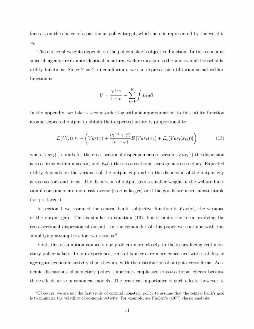
In the appendix, we take a second-order logarithmic approximation to this utility function
around expected output to obtain that expected utility is proportional to:
E(U(.)) ≈ −µV ar(x) +
(γ−1 + ψ)
(σ + ψ)E [V ark(xk) + Ek(V ari(xki))]
¶(13)
where V ark(.) stands for the cross-sectional dispersion across sectors, V ari(.) the dispersion
across firms within a sector, and Ek(.) the cross-sectional average across sectors. Expected
utility depends on the variance of the output gap and on the dispersion of the output gap
across sectors and firms. The dispersion of output gets a smaller weight in the welfare func-
tion if consumers are more risk averse (so σ is larger) or if the goods are more substitutable
(so γ is larger).
In section 1 we assumed the central bank’s objective function is V ar(x), the variance
of the output gap. This is similar to equation (13), but it omits the term involving the
cross-sectional dispersion of output. In the remainder of this paper we continue with this
simplifying assumption, for two reasons.6
First, this assumption connects our problem more closely to the issues facing real mon-
etary policymakers. In our experience, central bankers are more concerned with stability in
aggregate economic activity than they are with the distribution of output across firms. Aca-
demic discussions of monetary policy sometimes emphasize cross-sectional effects because
these effects arise in canonical models. The practical importance of such effects, however, is
6Of course, we are not the first study of optimal monetary policy to assume that the central bank’s goalis to minimize the volatility of economic activity. For example, see Fischer’s (1977) classic analysis.
11

open to debate.
Second, the simpler objective function allows us to establish some theoretical results
which are intuitive and easy to interpret. Extending the results to the case where the central
bank takes both terms into account in designing optimal policy would certainly be a useful
exercise, but the extra complexity would likely preclude clean analytic results. In section 5
we compare our results to those obtained in papers that numerically worked with welfare
functions similar to that in equation (13).
The bottom line from this analysis is that the stability-price-index problem stated in
Section 1 is closely related to a reduced form of a model of price adjustment under monop-
olistic competition. The canonical models in this literature assume symmetry across sectors
in order to keep the analysis simple (e.g., Blanchard and Kiyotaki, 1987; Ball and Romer,
1990). Yet sectoral differences are at the heart of our problem. Therefore, we have extended
the analysis to allow for a rich set of sectoral characteristics, which are described by the
parameters θk, αk, λk, and σ2k.
3 The Two-Sector Solution
We are now interested in solving the central bank’s problem. To recap, it is:
min{ωk}
V ar(x)
subject to
KXk=1
ωkpk = 0
KXk=1
ωk = 1
pk = λkp∗k + (1− λk)E(p
∗k)
p∗k = p+ αkx+ εk
p =KXk=1
θkpk.
12

The central bank chooses a target price index to minimize output volatility, given the con-
straints imposed by the price-setting process.
To illustrate the nature of the solution, we now make the simplifying assumptions that
there are only two sectors (K = 2), which we call sector A and sector B, and that the shocks
to each sector (εA and εB) are uncorrelated. We also assume that αA and αB are both
nonnegative. Appendix 2 derives the solution to this special case. The conclusion is the
following equation for the optimal weight on sector A:
ω∗A = λBαAσ
2B − θAλA (αAσ
2B + αBσ
2A)
αBλA(1− λB)σ2A + αAλB(1− λA)σ2B.
Notice that the optimal target weight depends on all the sectoral characteristics and, in
general, need not be between zero and one.
From this equation, we can derive several propositions that shed light on the nature of
the solution. We begin with a very special case. Of course, if the two sectors are identical
(same θk, αk, λk, and σ2k), then the stability price index gives them equal weight (ω∗k = 1/2).
This result is not surprising, as it merely reflects the symmetry of the two sectors.
More interesting results arise when the sectoral characteristics (θk, αk, λk, and σ2k) vary.
Let’s start with the two characteristics that describe equilibrium prices.
Proposition 1 An increase in αk raises the optimal ωk. That is, the more responsive
a sector is to the business cycle, the more weight that sector’s price should receive in the
stability price index.
Proposition 2 An increase in σ2k reduces the optimal ωk. That is, the greater the magnitude
of idiosyncratic shocks in a sector, the less weight that sector’s price should receive in the
stability price index.
Both of these propositions can be viewed from a signal-extraction perspective: A sector’s
price is useful for a central bank when its signal about the output gap is high (as measured
by αk) and when its noise is low (as measured by σ2k). Propositions 1 and 2 both coincide
with aspects of the conventional wisdom. When economists point to commodity prices as a
useful economic indicator for monetary policy, they usually do so on the grounds that these
13

prices are particularly responsive to the business cycle. The index of leading indicators, for
instance, includes the change in “sensitive materials prices.” Proposition 1 can be used to
justify this approach. At the same time, when economists reduce the weight they give to
certain sectors, as they do with food and energy sectors in the computation of the core CPI,
they do so on the grounds that these sectors are subject to particularly large sector-specific
shocks. Proposition 2 can be used to justify this approach.
Let’s now consider the effects of price sluggishness on the optimal target weights:
Proposition 3 If the optimal weight for a sector is less than 100 percent (ωk < 1), then
an increase in λk reduces the optimal ωk. That is, the more flexible a sector’s price, the less
weight that sector’s price should receive in the stability price index.
As earlier, some intuition for this result comes from thinking about the problem from a
signal-extraction perspective. Price stickiness dampens the effect of the business cycle on
a sector’s price. Conversely, when prices are very sticky, a small price movement signals a
large movement in the sector’s desired price, which in turn reflects economic activity. An
optimizing central bank offsets the effect of this dampening from price stickiness by giving
a greater weight to stickier sectors.
A special case is noteworthy:
Proposition 4 If the two sectors are identical in all respects except one has full price
flexibility prices (same αk, θk, and σ2k but λA = 1, λB < 1), then the monetary authority
should target the price level in the sticky-price sector (ωB = 1).
This result is parallel to that presented by Aoki (2001). But the very strong conclusion
that the central bank should completely ignore the flexible-price sector does not generalize
beyond the case of otherwise identical sectors. Even if a sector has fully flexible prices, the
optimal target weight for that sector is in general nonzero.
The last sectoral characteristic to consider is θk, the weight that the sector receives in
the consumer price index.
Proposition 5 An increase in θk reduces the optimal ωk. That is, the more important a
price is in the consumer price index, the less weight that sector’s price should receive in the
14

stability price index.
This proposition is probably the least intuitive one. It illustrates that choosing a price index
to aim for economic stability is very different than choosing a price index to measure the
cost of living.
What is the intuition behind this surprising result? Under inflation targeting, undesirable
fluctuations in output arise when there are shocks εk to equilibrium prices, which the central
bank has to offset with monetary policy. The effect of a shock in sector k depends on the
consumption weight θk. The greater is the consumption weight, the more the shock feeds into
other prices in the economy, and the more disruptive it is. Thus, to minimize the disruptive
effect of a shock, a central bank should accommodate shocks to large sectors. Under inflation
targeting, such accommodation is possible by reducing the weight of the sector in the target
index. Hence, holding all the other parameters constant, sectors with a larger weight in the
consumption index should receive a smaller weight in the target index.7
To sum up, the ideal sectoral prices for a central bank to monitor are those that are highly
sensitive to the economy (large αk), experience few sectoral shocks (small σ2k), have very
sluggish prices (low λk), and are relatively small in the aggregate price index (small θk). It
is important to acknowledge, however, that these results depend on the assumption that the
correlation between the εk is zero. With a general covariance matrix, only two propositions
survive. Proposition 1 still holds since one can show that ∂ωk/∂αk ≥ 0, so the optimal
target weight does not decrease as a sector’s cyclical sensitivity increases. Moreover, if the
sectors are identical in all respects except that in one sector prices are fully flexible, optimal
policy targets the sticky price alone, as in Proposition 4. In the empirical application below,
however, we find that the off-diagonal elements of the covariance matrix do not influence
the most important conclusions. So perhaps the special case highlighted in Propositions 1
through 5 is empirically plausible.
Another noteworthy special case is the one in whichP
θkεk = 0. In the microfoundations
developed in Section 2, this case arises if there are productivity shocks but no markup shocks.
7The idea of giving a large weight to a small sector may sound implausible at first, but that is preciselythe policy that many nations adopted during the nineteenth century. Under a gold standard, the small goldsector receives a target weight of 100 percent.
15

In this special case, one can show that
ω∗A = θAλB (1− λA)
λA(1− λB) + θA(λB − λA). (14)
The optimal target weight rises with decreases in λk as before, but now it rises with increases
in θA. These results are parallel to those in Benigno (2001). In addition, if one sector has
flexible prices, then optimal policy targets the sticky-price sector. This case corresponds
most closely to the one studied by Aoki (2001).
4 Toward Implementation: An Example
The two-sector example considered in the previous section is useful for guiding intuition, but
if a central bank is to compute a stability price index, it will need to go beyond this simple
case. In this section, we take a small step toward a more realistic implementation of the
stability price index.
4.1 The Approach
We apply the model to annual data for the U.S. economy from 1957 to 2001. We examine four
sectoral prices: the price of food, the price of energy, the price of other goods and services,
and the level of nominal wages. The first three prices are categories of the consumer price
index, while wages refer to compensation per hour in the business sector. As a proxy for
the output gap, we use twice the deviation of unemployment from its trend value, where the
trend is computed using the Hodrick-Prescott filter.8 All series come from the Bureau of
Labor and Statistics.
A key question is how to assign parameters to the four sectors. We begin by noting the
following equation holds in the model:
pk − Epk = λk(p− Ep) + αkλk(x− Ex) + λk(εk −Eεk) (15)
8The factor of two corrects for an Okun’s law relationship and only affects the estimated αk but not thetarget weights. We also tried estimating x using detrended output and obtained similar results.
16

That is, the price surprise in sector k is related to the overall price surprise, the output
surprise, and the shock. To obtain these surprise variables, we regressed each of the variables
pk, p, and x on three of its own lags, a constant, and a time trend and took the residual.
These surprise variables are the data used in all subsequent calculations.
In principle, one should be able to obtain the parameters by estimating equation (15).
In practice, the identification problem makes formal estimation difficult. Shocks (such as an
energy price increase) will likely be correlated with the overall price level and the level of
economic activity. Finding appropriate instruments is a task we leave for future work. Here,
as a first pass, we adopt a cruder approach that is akin to a back-of-the-envelope calculation.
For the parameter λk, which governs the degree of price sluggishness, we rely on bald,
but we hope realistic, assumptions. We assume the food and energy prices are completely
flexible, so λk = 1. Other prices and wages are assumed to be equally sluggish. We set
λk = 1/2, indicating that half of price setters in these sectors base their prices based on
expected, rather than actual, economic conditions.
Another key parameter is αk, the sensitivity of desired prices to the level of economic
activity. We estimate this parameter by assuming that the 1982 economic downturn — the
so-called Volcker recession — was driven by monetary policy, rather than sectoral supply
shocks. Thus, we pick αk for each sector so that equation (15) without any residual holds
exactly for 1982. That is, we are using the price responses during the 1982 recession to
measure the cyclical sensitivity of sectoral prices.
With αk and λk, we can compute a time series of εk − Eεk and, thus, its variance-covariance matrix. Note that we do not assume that the shocks are uncorrelated across
sectors. The previous section made this assumption to obtain easily interpretable theoretical
results, but for a more realistic numerical exercise, it is better to use the actual covariances.
Thus, if there is some shock that influences desired prices in all sectors (for a given p and
y), this shock would show up in the variance-covariance matrix, including the off-diagonal
elements.
The last parameter is the consumption weight θk. We take this parameter from the
“relative importance” of each sector in the consumer price index as determined by the Bureau
of Labor Statistics. For nominal wages, θk is equal to zero, because nominal wages do not
17

appear in the consumer price index.
With all the parameters in hand, it is now a straightforward numerical exercise to find
the set of target weights ωk that solves the stability-price-index problem as set forth above.
Appendix 3 describes the algorithm.
4.2 The Results
Table 1 presents the results from this exercise. The column denoted ωc imposes the constraint
that all the sectoral weights in the stability price index be nonnegative. The column denoted
ωu, allows the possibility of negative weights. The substantive result is similar in the two
cases: The price index that the central bank should use to maximize economic stability gives
most of its weight to the level of nominal wages.
The intuition behind this result is easy to see. The value of αk for nominal wages is 0.29,
which is larger than the parameter for most other sectors. (This parameter value reflects
the well-known fact that real wages are procyclical.9) The only other sector that exhibits
such a large value of αk is the energy sector. But the variance of shocks in the energy sector,
measured by V ar(εk), is very large, making it an undesirable sector for the stability price
index. The combination of high αk and low V ar(εk) makes nominal wages a particularly
useful addition to the stability price index.10
One might suspect that the zero value of θk for nominal wages in the consumer price
index is largely responsible for the high value of ωk in the stability price index. That turns
out not to be the case. Table 2 performs the same empirical exercise as in Table 1, but it
assumes that the economy’s true price index gives half its weight to nominal wages (that is,
p = 0.5w + 0.5cpi). Once again, the most important element of the stability price index is
the level of nominal wages.11
9The estimate of the procyclicality of real wages we obtained here is similar to those found in otherstudies. Because αk for nominal wages exceeds the αk for other goods by 0.19, the desired real wage rises by0.19 percent for every 1 percentage point increase in the output gap. If λk equals 0.5 for these two sectors,as we have assumed, then the actual real wage would rise by 0.095. For comparison, Solon, Barsky, andParker (1994) estimate the elasticity of real wages with respect to output in aggregate data is 0.146.10Indeed, if a better index of wages were available, it would likely be more procyclical, reinforcing our
conclusion. See Solon, Barsky, and Parker (1994) on how composition bias masks some of the procyclicalityof real wages.11How is the approximate irrelevance of θk here consistent with Proposition 5? The proposition examines
18

Two other striking results in Table 1 are the large weight on the price of food and
the large, negative weight on the price of goods other than food and energy. These results
depend crucially on the pattern of correlations among the estimated shocks. The last column
in Tables 1 and 2, denoted ω0 sets these correlations to zero. The target weights for food and
other goods are much closer to zero (while the target weight for nominal wages remains close
to one).12 In light of this sensitivity, this aspect of the results should be treated with caution.
One clear lesson is that the variance-covariance matrix of the shocks is a key input into the
optimal choice of a price index. The large weight on nominal wages, however, appears robust.
It is worth noting that the gain in economic stability from targeting the stability price
index rather than the consumer price index is large. It is straightforward to calculate the
variance of output under each of the two policy rules. According to this model, moving from
a target for the consumer price index to a target for the stability price index reduces the
output gap variance by 53 percent (or by 49 percent with a nonnegativity constraint on the
weights). Thus, the central bank’s choice of a price index to monitor inflation is an issue of
substantial economic significance.
A natural extension to this exercise would be to include asset prices, such as the price of
equities. Although stock prices experience large idiosyncratic shocks (high σ2k), they are also
very cyclically sensitive (high αk). As a result, it is plausible that the stability price index
should give some weight to such asset prices. When we added the S&P 500 price index to
the sectoral prices used in Table 1, it received a target weight that was positive and around
0.2. The target weight on nominal wages remained large.
Finally, we should emphasize how tentative these calculations are. Our attempt at mea-
suring the key sectoral parameters is certainly crude. Future work could aim at finding better
econometric techniques to measure these parameters. Once credible estimation procedures
what happens to ωk when θk changes, holding constant other parameter values. But in this empiricalexercise, if we change the weight given to some sector in the price index p, we also change the estimatedvalues of αk and the variance-covariance matrix of εk.12Although it is not easy to gain intuition for why the off-diagonal elements of the covariance matrix have
the effect they do, here is our conjecture: The largest correlation in Table 1 is the 0.30 between the shock towages and the shock to the prices of other goods. Thus, the stability price index, which gives a high weightto wages, tries to “purge” the shock to wages by giving a negative weight to the price of other goods. Moregenerally, when there is correlation among sectors, the stability price index tries to choose the combinationof prices such that shocks among the sectors are offsetting in the overall index.
19

are in hand, one could expand the list of candidate prices.
20

Table 1
Results of Empirical Illustration
Sector λ α V ar(ε) θ ωu ωc ω0
Energy 1.0 0.37 0.00279 0.07 0.10 0.03 0.01
Food 1.0 0.10 0.00025 0.15 0.37 0.21 0.10
Other Goods 0.5 0.10 0.00016 0.78 -0.73 0 -0.07
Wages 0.5 0.29 0.00050 0 1.26 0.76 0.96
Correlation Matrix of Epsilon
Energy Food Other
Goods
Wages
Energy 1.00 -0.27 0.19 -0.17
Food 1.00 -0.24 0.03
Other Goods 1.00 0.30
Wages 1.00
21
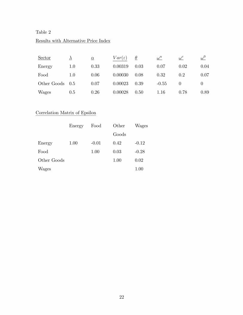
Table 2
Results with Alternative Price Index
Sector λ α V ar(ε) θ ωu ωc ω0
Energy 1.0 0.33 0.00319 0.03 0.07 0.02 0.04
Food 1.0 0.06 0.00030 0.08 0.32 0.2 0.07
Other Goods 0.5 0.07 0.00023 0.39 -0.55 0 0
Wages 0.5 0.26 0.00028 0.50 1.16 0.78 0.89
Correlation Matrix of Epsilon
Energy Food Other
Goods
Wages
Energy 1.00 -0.01 0.42 -0.12
Food 1.00 0.03 -0.28
Other Goods 1.00 0.02
Wages 1.00
22

5 Relationship to the previous literature
The idea that a central bank should look beyond the consumer price index when monitoring
inflation is not a new one. For example, in 1978 Phelps concluded, “the program envisioned
here aims to stabilize wages on a level or a rising path, leaving the price level to be buffeted by
supply shocks and exchange-rate disturbances.”13 In Mankiw and Reis (2001b) we explored
a model that supports Phelps’s policy prescription. That model can be viewed as a special
case of the stability-price index framework considered here, with some strong restrictions
on the parameter values. If sector A is the labor market and sector B is the goods market,
then the earlier model can be written in a form such that θA = 1, λB = 1, αB = 0, and
σ2A = 0. In this special case, the equation for the optimal target weight immediately implies
that ω∗A = 1.
Erceg, Henderson and Levin (2000) have recently also found that optimal monetary
policy can be closely approximated by targeting the nominal wage. Their analysis differs
substantially from ours. Whereas our calculations in Section 4 treat wages in exactly the
same way as any other sectoral price, Erceg et al focus instead on the specific features of
the labor market, where nominal rigidities induce distortions in labor-leisure choices and
shocks feed into the other sectors in the economy via wages and costs. Our argument for
nominal wage targeting can be seen as complementary to theirs, further strengthening their
conclusion.
The modern literature has also recently taken up the question of how should monetary
policy be set if there are different sectors in the economy. Aoki (2001) studies optimal
monetary policy in an economy with two sectors: one with perfectly flexible prices and the
other with some nominal rigidity. He finds that the central bank should target the sticky-
price sector only. We obtain this same result, but only in the special cases either where the
two sectors were identical in all other respects, as stated in proposition 4, or where there are
only productivity shocks.
Benigno (2001) focuses instead on the problem facing a currency union with two regions.
Even though his model has richer microfoundations than ours, we are able to reproduce two of
13Phelps has told us that this idea dates back to Keynes, but we have not been able to find a reference.
23

his main conclusions within our simple framework. Benigno does not include markup shocks,
focussing only on the presence of disturbances that correspond to our productivity shocks.
He finds that the larger is the weight of a sector in the economy, the larger the weight it should
receive in the stability price index, as we found in Section 3 when only productivity shocks
were present. In addition, he shows that if the degree of nominal rigidity in the two sectors
is the same, then the optimal policy is to target the CPI, regardless of any other differences
between the sectors. If there are only productivity shocks, our model leads to this conclusion
as well. Both Aoki and Benigno used models different from ours, notably by introducing
nominal rigidities in the form of Calvo staggered pricing rather than pre-determined prices
as we do,14 and by using a different objective function for the policymaker. Nonetheless,
their conclusions carry over to our setting.
6 Conclusion
Economists have long recognized that price indices designed to measure the cost of living
may not be the right ones for the purposes of conducting monetary policy. This intuitive
insight is behind the many attempts to measure “core inflation.” Yet, as Wynne (1999)
notes in his survey of the topic, the literature on core inflation has usually taken a statistical
approach without much basis in monetary theory. As a result, measures of core inflation
often seem like answers in search of well-posed questions.
The price index proposed in this paper can be viewed as an approach to measuring core
inflation that is grounded in the monetary theory of the business cycle. The stability price
index is the weighted average of prices that, if kept on target, leads to the greatest stability
in economic activity. The weights used to construct such a price index depend on sectoral
characteristics that differ markedly from those relevant for measuring the cost of living.
Calculating a stability price index is not an easy task. Measuring all the relevant sectoral
characteristics is an econometric challenge. Moreover, there are surely important dynamics in
the price-setting decision that we have omitted in our simple model. Yet, if the calculations
14For a comparison of the different properties of “sticky price” and “sticky information” models of nominalrigidities, see Mankiw and Reis (2001a).
24

performed in this paper are indicative, the topic is well worth pursuing. The potential
improvement in macroeconomic stability from targeting the optimal price index, rather than
the consumer price index, appears large.
Our results suggest that a central bank that wants to achieve maximum stability of
economic activity should give substantial weight to the growth in nominal wages when mon-
itoring inflation. This conclusion follows from the fact that wages are more cyclically sensitive
than most other prices in the economy (which is another way of stating the well-known fact
that the real wage is procyclical). Moreover, compared to other cyclically sensitive prices,
wages are not subject to large idiosyncratic shocks. Thus, if nominal wages are falling rela-
tive to other prices, it indicates a cyclical downturn, which in turn calls for more aggressive
monetary expansion. Conversely, when wages are rising faster than other prices, targeting
the stability price index requires tighter monetary policy than does conventional inflation
targeting.
An example of this phenomenon occurred in the United States during the second half of
the 1990s. Here are the U.S. inflation rates as measured by the consumer price index and
an index of compensation per hour:
Year CPI Wages
1995 2.8 2.1
1996 2.9 3.1
1997 2.3 3.0
1998 1.5 5.4
1999 2.2 4.4
2000 3.3 6.3
2001 2.8 5.8
Consider how a monetary policymaker in 1998 would have reacted to these data. Under
conventional inflation targeting, inflation would have seemed very much in control, as the
CPI inflation rate of 1.5 percent was the lowest in many years. By contrast, a policymaker
trying to target a stability price index would have observed accelerating wage inflation. He
would have reacted by slowing money growth and raising interest rates (a policy move that in
25

fact occurred two years later). Would such attention to a stability price index have restrained
the exuberance of the 1990s boom and avoided the recession that began the next decade?
There is no way to know for sure, but the hypothesis is intriguing.
26

Appendix 1 - Approximation of the utility function
In this appendix, following Woodford (2002), we derive the objective function of the
policymaker as a Taylor second-order log-linear approximation of the utility function. This
extends the multi-sector analysis of Benigno (2001) to the case where there are markup
shocks in addition to productivity shocks.
The first issue to address is the choice of the point around which to linearize. Following
the literature, we linearize around the steady state equilibrium of the economy with flexible
prices and no real disturbances, so that all shocks are at their means. As Woodford discusses,
it is important for the accuracy of the log-linearization that this is close enough to the efficient
equilibrium of the economy. To ensure this is the case, we assume the average markup is
one for all sectors: E(mk) = 1. One way to make this consistent with the monopolistic
competition model is to introduce a production subsidy to firms funded by lump-sum taxes
on consumers15.
In order to interpret θk as the share of a sector in total output, units must be chosen
appropriately so that all steady state equilibrium sectoral prices pk are the same. From eq.
(10), this requires that units of measurement be such that average productivity respects the
condition:
ak = − (σ + ψ) y − ψ log(θk). (A.1)
The y must be the same across sectors, and corresponds to the level of aggregate output
around which we linearize y. From the demand functions in equation (7), the equilibrium
firm and sector output levels are yki = yk = y + log(θk).
We can now turn to the linearization of the utility function:
U(.) =Y 1−σ
1− σ−
KXk=1
Z 1
0
Lkidi, (A.2)
which we do in a sequence of steps.
Step 1: Approximating Y 1−σ/ (1− σ)
15Alternatively we could allow the markups to be of first or higher stochastic order.
27

A second-order linear approximation of y around y, letting y = y − y yields
Y 1−σ
1− σ=
e(1−σ)y
1− σ
≈ e(1−σ)y
1− σ
Ã1 + (1− σ) y +
(1− σ)2
2y2
!
≈ e(1−σ)yµy +
1− σ
2y2¶. (A.3)
The approximation in the last line involves dropping a term that enters the expression
additively and which the policymaker can not affect. Therefore, it does not influence the
results from the optimization and can be dropped.
Step 2: Approximating Lki
Inverting the production function in (6) we obtain:
Lki =eak
1 + ψY 1+ψki .
A first-order approximation of this around yki and ak, letting yki = yki− yki and ak = ak− akleads to:
Lki =1
1 + ψeak+(1+ψ)yki
≈ eak+(1+ψ)yki
1 + ψ(1 + ak +
1
2a2k +
(1 + ψ)yki +(1 + ψ)2
2y2ki + (1 + ψ)akyki)
≈ eak+(1+ψ)ykiµyki +
1 + ψ
2y2ki + akyki
¶,
where again in the last line, we drop additive constants that are independent of policy.
Step 3: Integrating to obtainRLkidi.
Integrating the previous expression over the farmers i in sector k, leads to:
ZLkidi =
Zeak+(1+ψ)yki
µyki +
1 + ψ
2y2ki + akyki
¶di.
Since yki = yk, and denoting by Ei(yki) =Rykidi the cross-sectional average of output across
28

firms in sector k, we obtain:
ZLkidi = e
ak+(1+ψ)yk
µEi(yki) +
1 + ψ
2Ei(y
2ki) + akEi(yki)
¶.
From the definition of the cross-sectional variance, V ari(yki) = Ei(y2ki)− Ei(yki)2, so:ZLkidi = e
ak+(1+ψ)yk
µEi(yki) +
1 + ψ
2
¡V ari(yki) + Ei(yki)
2¢+ akEi(yki)
¶. (A.4)
Next, realize that a second-order approximation of the CES aggregator in equation (5),
around yki = yk yields:
Ei(yki) ≈ yk − 1− γ−1
2V ari(yki).
Using this expression to substitute for Ei(yki) in equation (A.4), rearranging and dropping
third or higher order terms, we obtain:
ZLkidi = e
ak+(1+ψ)yk
µyk +
1 + ψ
2y2k +
γ−1 + ψ
2V ari(yki) + akyk
¶.
Step 4: Adding to obtainPR
Lkidi.
Adding up the expression above over the k sectors, we obtain:
KXk=1
ZLkidi =
KXk=1
eak+(1+ψ)ykµyk +
1 + ψ
2y2k +
γ−1 + ψ
2V ari(yki) + akyk
Since yk = y + log(θk) equation (A.1), implies that ak + (1 + ψ)yk = (1 − σ)y + log(θk).
Therefore:
KXk=1
ZLkidi = e(1−σ)y
KXk=1
θk
µyk +
1 + ψ
2y2k +
γ−1 + ψ
2V ari(yki) + akyk
¶= e(1−σ)y
µEk(yk) +
1 + ψ
2Ek(y
2k) +
γ−1 + ψ
2Ek(V ari(yki)) + Ek(akyk)
¶,
where the cross-sectional average of output across sectors is denoted by: Ek(yk) =PK
k=1 θkyk.
Approximating the terms in the CES aggregator in equation (4) around yk = y+ log(θk)
29

we obtain:
Ek(yk) ≈ y − 1− γ−1
2V ark(yk). (A.5)
Using this to replace for Ek(yk) in the expression above and dropping third or higher order
terms leads to:
KXk=1
ZLkidi ≈ e(1−σ)y
µy +
1 + ψ
2y2 +
(γ−1 + ψ)
2[V ark(yk) + Ek(V ari(yki))] + Ek(akyk)
¶.
(A.6)
Step 5: Combining all the previous steps.
The second-order approximation of the utility function (A.2) is given by the sum sub-
tracting the result in (A.6) from (A.3). Cancelling terms we obtain:
U ≈ −e(1−σ)y (σ + ψ)
2
µy2 + 2
Ek(akyk)
(σ + ψ)+(γ−1 + ψ)
(σ + ψ)[V ark(yk) + Ek(V ari(yki))]
¶.
Now focus on the term Ek(akyk). From (A.5), it is clear that yEk(ak) ≈ Ek(ak)Ek(yk),up to second-order terms. Therefore:
Ek(akyk) = yEk(ak) + Ek(akyk)− yEk(ak)≈ yEk(ak) + Ek [(ak − Ek(ak))(yk −Ek(yk))]
From the definition of the natural rate in eq. (11), we can replace Ek(ak) in the expression
above to obtain:
Ek(akyk) = −y(σ + ψ)yN + Covk(ak, yk),
where Covk(ak, yk) = Ek [(ak − Ek(ak))(yk −Ek(yk))] stands for the cross-sectional covari-ance. Using this to replace for Ek(akyk) in our approximation of the utility function, and
adding a term involving yN (which is beyond the control of policy so leaves the maximization
30

problem unchanged), leads to:
U ≈ −e(1−σ)y (σ + ψ)
2
µ¡y − yN¢2 + (γ−1 + ψ)
(σ + ψ)
·2Covk(ak, yk)
(γ−1 + ψ)+ V ark(yk) + Ek(V ari(yki))
¸¶.
Next, we simplify the term in the square brackets above. Since V ark(ak)/ (γ−1 + ψ)2 is
beyond the control of the monetary policy, we can add it to the term in brackets in the
utility function to obtain:
2Covk(ak, yk)
(γ−1 + ψ)+ V ark(yk) ≈ V ark
½yk +
ak(γ−1 + ψ)
¾. (A.7)
Now, we calculate the natural rate of output in each sector. From the demand functions in
(7), taking logs, at the natural rate equilibrium:
yNk = −γ(pNk − pN) + log(θk) + yN .
Subtracting yk = log(θk) + y we obtain:
yNk = −γ(pNk − pN) + yN . (A.8)
From the pricing condition (10) and since at the natural rate equilibrium prices are flexible,
and markups are 1:
(1 + γψ)(pNk − pN) = (σ + ψ)yN + ak + ψ log(θk).
At the point of linearization, the condition above also holds but with the stochastic variable
ak replaced by its mean ak. In terms of deviations from the equilibrium around which we
linearize, the expression above becomes:
(1 + γψ)(pNk − pN ) = (σ + ψ)yN + ak. (A.9)
31

Combining (A.8) and (A.9) substituting out for relative prices, we obtain:
− akγ−1 + ψ
= yNk +σ − γ−1
γ−1 + ψyN .
The expression in (A.7) can therefore be re-written as:
V ark(yk − yNk )
Going back to the utility function we then have:
U ≈ −e(1−σ)y (σ + ψ)
2
µ¡y − yN¢2 + (γ−1 + ψ)
(σ + ψ)
£V ark(yk − yNk ) + Ek(V ari(yki))
¤¶.
We drop the hats from y−yN and yk−yNk since the conditions defining the equilibrium aroundwhich we linearize include the conditions defining the natural rate equilibrium. Finally, using
the assumption that E(mk) = 1 made in the beginning of the appendix, the model in section
1 implies that E¡y) ≈ E(yN¢. This holds only up to second-order terms, since we use first-
order approximations to obtain the price index of the economy and the resultE(log(mk)) ≈ 0.Taking expectations of the equation above, and dropping the proportionality factor that is
outside the influence of the policymaker, we can write the objective of the policymaker
setting his rule before observing the shocks as:
E(U) ≈ −µV ar(y − yN) + (γ
−1 + ψ)
(σ + ψ)E£V ark(yk − yNk ) + Ek(V ari(yki))
¤¶.
Finally, note that yki = yk for all i, so we can add it to the last cross-sectional variance term.
Moreover yNki = yNk since with perfect price flexibility all firms within a sector are identical
and so have the same natural rate of output. We can therefore replace all output variables
by gap variables in the expression above to obtain equation (13) in the text.
Appendix 2 - Results for the two-sector case
In this appendix, we prove the results and propositions presented in section 3 of the text.
The optimal weights in the Stability Price Index
32

First, express all variables as deviations from their expected value. Letting a tilde over
a variable denote its deviations from its expected value (x = x − E(x)), the model can bewritten as:
p∗k = p+ αkx+ εk
pk = λkp∗k + (1− λk)E(p
∗k)
p = θApA + θBpB
0 = ωApA + ωBpB.
Next, we use the facts that (i) there are only 2 sectors in this application (k = A,B), (ii)
the expected value of any variable with a tilde over it is zero, and (iii) the weights must sum
to one, to re-express the system as:
pA = λA (p+ αAx+ εA)
pB = λB (p+ αBx+ εB)
p = θApA + (1− θA)pB
0 = ωApA + (1− ωA)pB.
This is a system of 4 equations in 4 variables (pA, pB, p, x). Solving for the variable of interest
x, we obtain:
x = − [ωA + λB (θA − ωA)]λAεA + [(1− ωA)− λA(θA − ωA)]λB εBαBλB + ωA(αAλA − αBλB) + λAλB (ωA − θA) (αB − αA)
(A.10)
The policymaker will then choose the weight ωA in order to minimize the variance of the
expression above. Using the first-order condition and rearranging we find the optimal ω∗A
given by:
ω∗A = λBαAσ
2B − θAλA (αAσ
2B + αBσ
2A)
αBλA(1− λB)σ2A + αAλB(1− λA)σ2B(A.11)
The optimal ω∗B is just given by ω∗B = 1− ω∗A.
33

Proof of the Propositions
Special case: Using the values αA = αB, σ2A = σ2B, λA = λB, θA = θB = 1/2 in the
formula for ω∗A above we find that ω∗A = 1/2.
Proposition 1: Taking derivatives of (A.11) with respect to αA, we find that
∂ω∗A∂αA
=αBλAλBσ
2Aσ
2B(1− θAλA − (1− θA)λB)
(αBλA(1− λB)σ2A + αA(1− λA)λBσ2B)2
The denominator is clearly non-negative, and so is the numerator since λk ≤ 1 and θk ≤ 1,so we can sign ∂ω∗A/∂αA ≥ 0. By symmetry ∂ω∗B/∂αB ≥ 0.Proposition 2: Taking derivatives of the solution (A.11):
∂ω∗A∂σ2A
= − αAαBλAλBσ2B(1− θAλA − (1− θA)λB)
(αBλA(1− λB)σ2A + αA(1− λA)λBσ2B)2
which by the same argument as in the previous proposition, implies ∂ω∗A/∂σ2A ≤ 0 (and
∂ω∗B/∂σ2B ≤ 0 symmetrically).
Proposition 3: Taking derivatives of ω∗A with respect to λA:
∂ω∗A∂λA
= −αAλBσ2B [αBσ
2A − (1− θA)λB(αBσ
2A + αAσ
2B)]
(αBλA(1− λB)σ2A + αA(1− λA)λBσ2B)2 .
From the solution for ω∗A:
ω∗A < 1⇔αBσ
2A > (1− θA)λB(αBσ
2A + αAσ
2B).
Therefore, as long as ω∗A < 1, then ∂ω∗A/∂λA < 0. By symmetry it follows that ∂ω
∗B/∂λB < 0.
Proposition 4: Follows from evaluating the optimal solution ω∗A at the point: αA = αB,
σ2A = σ2B, θA = θB = 0.5, λA = 1, λB < 1, to obtain ω∗A = 0.
Proposition 5: Taking derivatives of ω∗A with respect to θA, we obtain:
∂ω∗A∂θA
= − λAλB(αBσ2A + αAσ
2B)
αBλAσ2A(1− λB) + αAλBσ2B(1− λA),
34

which is negative. Clearly ∂ω∗B/∂θB is also negative.
The Stability Price Index with an unrestricted shock covariance matrix
Minimizing the variance of equation (A.10) we obtain the optimal weight on sector A:
ω∗A = λBαA [σ
2B + θAλA(σAB − σ2B)]− αB [θAλA(σ
2A − σAB) + σAB]
αA [(1− λA)λBσ2B − λA(1− λB)σAB] + αB [(1− λB)λAσ2A − λB(1− λA)σAB],
(A.11)
where σAB denotes the covariance between εA and εB. Taking derivatives of (A.11) with
respect to αA we find:
∂ω∗A∂αA
=αBλAλB(1− θAλA − (1− θA)λB)(σ
2Aσ
2B − σ2AB)
(αA [(1− λA)λBσ2B − λA(1− λB)σAB] + αB [(1− λB)λAσ2A − λB(1− λA)σAB])2 .
Clearly ∂ω∗A/∂αA ≥ 0, and by symmetry ∂ω∗B/∂αB ≥ 0, so proposition 1 still holds.Evaluating the optimal solution ω∗A in equation (A.10) at the point: αA = αB, σ2A = σ2B,
θA = θB = 0.5, λA = 1, λB < 1, we obtain ω∗A = 0, so proposition 4 still holds.
Appendix 3 - Multi-sector problems
In this appendix, we describe how to find the optimal price index in a K sector problem
as in section 4 of the text. The algorithm has 3 steps. First, we solve for the equilibrium
output in the economy, by solving the set of K + 2 equations:
pk = λk(p+ αkx+ εk), k = 1, ..., K
p =KXk=1
θkpk
0 =KXk=1
ωkpk.
in K + 2 variables (x, p, and the pk), for the variable x, in terms of the parameters and the
innovations εk. Second, we take the unconditional expectation of the square of x, to obtain
the variance of output as a function of αk, θk, λk, ωk and the variances σ2k = E(ε2k) and
35

covariances σkj = E(εkεj):
V ar(x) = f(αk, θk,λk,ωk,σ2k, σkj).
Given values for (αk, θk, λk,σ2k,σkj) the third step is to numerically minimize f(.) with respect
to the ωk, subject to the constraint thatP
k ωk = 1, and possibly additional non-negativity
constraints: ωk ≥ 0.
36

References
[1] Aoki, Kosuke (2001) “Optimal monetary policy responses to relative-price changes,”
Journal of Monetary Economics, vol. 48, pp. 55-80.
[2] Ball, Laurence and David Romer (1990) “Real Rigidities and the Nonneutrality of
Money,” Review of Economic Studies, vol. 57, pp. 183-203.
[3] Benigno, Pierpaolo (2001) “Optimal Monetary Policy in a Currency Area,” CEPR Dis-
cussion Paper 2755.
[4] Blanchard, Olivier J. and Nobuhiro Kiyotaki (1987) “Monopolistic Competition and the
Effects of Aggregate Demand,” American Economic Review, vol. 77, pp. 647-666.
[5] Clarida, Richard, Jordi Gali and Mark Gertler (2002) “A Simple Framework for Interna-
tional Monetary Policy Analysis,” NBER Working Paper no. 8870. Carnegie-Rochester
Conference Series, forthcoming.
[6] Dixit, Avinash K. and Joseph E. Stiglitz (1977) “Monopolistic Competition and Opti-
mum Product Diversity,” American Economic Review, vol. 67, pp. 297-308.
[7] Erceg, Christopher J., Dale W. Henderson and Andre T. Levin (2000) “Optimal Mone-
tary Policy with StaggeredWage and Price Contracts,” Journal of Monetary Economics,
vol. 46, pp. 281-313.
[8] Fischer, Stanley (1977) “Long-Term Contracts, Rational Expectations, and the Optimal
Money Supply Rule,” Journal of Political Economy, vol. 85, pp. 191-205.
[9] Mankiw, N. Gregory and Ricardo Reis (2001a) “Sticky Information versus Sticky Prices:
A Proposal to Replace the New Keynesian Phillips Curve,” NBER Working Paper no.
8290. Quarterly Journal of Economics, forthcoming.
[10] Mankiw, N. Gregory and Ricardo Reis (2001b) “Sticky Information: A Model of Mone-
tary Nonneutrality and Structural Slumps,” NBERWorking Paper no. 8614. P. Aghion,
37
R. Frydman, J. Stiglitz and M. Woodford, eds., Knowledge, Information, and Expecta-
tions in Modern Macroeconomics: In Honor of Edmund S. Phelps, Princeton University
Press, forthcoming.
[11] Obstfeld, Maurice and Kenneth Rogoff (1996) Foundations of International Macroeco-
nomics, MIT Press: Cambridge.
[12] Phelps, Edmund S. (1978) “Disinflation without Recession: Adaptive Guideposts and
Monetary Policy,” Weltwirtschaftsliches Archiv, vol. 114 (4), pp. 783-809.
[13] Romer, David (2001) Advanced Macroeconomics. Second edition. McGraw-Hill.
[14] Rotemberg, Julio J. and Michael Woodford (1999) “The Cyclical Behavior of Prices and
Costs,” in J. B. Taylor and M. Woodford, eds., Handbook of Macroeconomics, vol. 1A,
Elsevier: Amsterdam.
[15] Solon, Gary, Robert B. Barsky, and Jonathan Parker (1994) “Measuring the Cyclical
Behavior of Real Wages: How Important is Composition Bias?” Quarterly Journal of
Economics, vol. 110 (2), pp. 321-352.
[16] Spence, Michael (1977) “Product Selection, Fixed Costs, and Monopolistic Competi-
tion,” Review of Economic Studies, vol. 43 (2), pp. 217-235.
[17] Steinsson, Jon (2002) “Optimal Monetary Policy in an Economy with Inflation Persis-
tence,” Journal of Monetary Economics, forthcoming.
[18] Woodford, Michael (2002) “Inflation Stabilization and Welfare,” Contributions to
Macroeconomics, The B.E. Journals in Macroeconomics, vol. 2 (1).
[19] Wynne, Mark A. (1999) “Core Inflation: A Review of Some Conceptual Issues,” ECB
Working Paper no. 5.
38