What Is a Structural Representation?

Lev Goldfarb, Oleg Golubitsky, Dmitry Korkin

Faculty of Computer ScienceUniversity of New Brunswick

Canada

October 25, 2001

Abstract

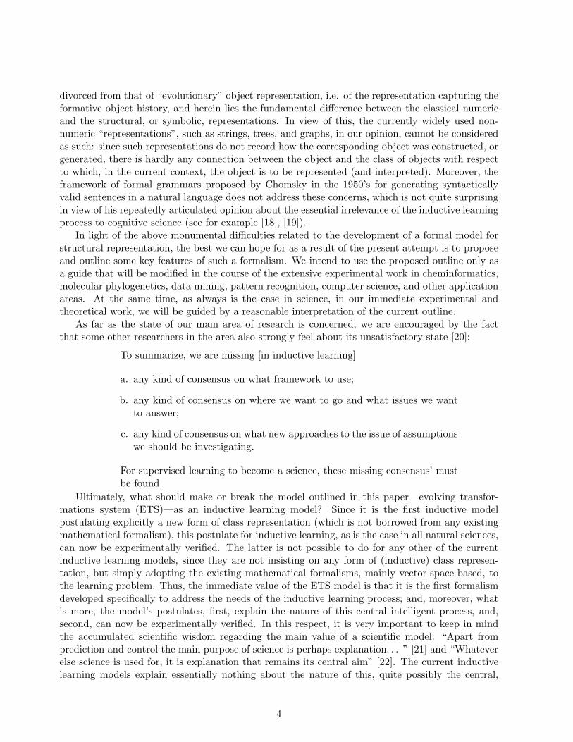
We outline a formal foundation for a “structural” (or “symbolic”) object/event representa-tion, the necessity of which is acutely felt in all sciences, including mathematics and computerscience. The proposed foundation incorporates two hypotheses: 1) the object’s formative historymust be an integral part of the object representation and 2) the process of object constructionis irreversible, i.e. the “trajectory” of the object’s formative evolution does not intersect itself.The last hypothesis is equivalent to the generalized axiom of (structural) induction. Some of themain difficulties associated with the transition from the classical numeric to the structural rep-resentations appear to be related precisely to the development of a formal framework satisfyingthese two hypotheses.

The concept of (inductive) class representation—which has inspired the development of thisapproach to structural representation—differs fundamentally from the known concepts of class.In the proposed, evolving transformations system (ETS), model, the class is defined by thetransformation system—a finite set of weighted transformations acting on the class progenitor—and the generation of the class elements is associated with the corresponding generative processwhich also induces the class typicality measure.

Moreover, in the ETS model, a fundamental role of the object’s class in the object’s repre-sentation is clarified: the representation of an object must include the class.

From the point of view of ETS model, the classical discrete representations, e.g. stringsand graphs, appear now as incomplete special cases, the proper completion of which shouldincorporate the corresponding formative histories, i.e. those of the corresponding strings orgraphs.

1

Concepts which have proved useful for ordinary things easily assume so greatan authority over us, that we forget their terrestrial origin and accept themas unalterable facts. They then become labeled as “conceptual necessities”,a priori situations, etc. The road of scientific progress is frequently blockedfor long periods by such errors.

A. Einstein

1 Introduction

In this paper, a vision of the concept of structural representation is outlined. On the one hand,although the overwhelming importance of structural, or symbolic, representations in all scienceshas become increasingly clear during the second half of the 20th century, there were hardly anysystematic attempts to address this topic at a fundamental level 1(and, from the point of viewof computer science, this is particularly puzzling in view of the central role played by the “datastructures” and “abstract data types” in computer science). On the other hand, it is not thatdifficult to understand the main reasons behind this situation. It appears that there are tworelated formidable obstacles to be cleared: 1) the choice of the central “intelligent” process, thestructure and requirements of which would both drive and justify the choice of the particular formof structural representation, and 2) the lack of any fundamental mathematical model whose rootsare not related to or motivated by the numeric models. Unfortunately, the role of the latter obstacleis usually completely underestimated. Why is it so? This is explained by the fact that during themankind’s scientific history, so far, we have dealt, basically, only with the numeric models and,during the last two centuries, with their derivatives. The latter should not be really surprising if welook carefully at the vast prehistory of science in general and of mathematics in particular [1],[2].The new level of mathematical abstractions and the excessive overspecialization (with the resultingnarrowing of the view) during the second half of the twentieth century have also contributed to thislack of understanding of the extent of our dependence on the numeric models. 2 What has begunto facilitate this understanding, however, is the emergence of computer “science” in general andartificial intelligence and pattern recognition (PR) in particular. (Although, for political reasons,during the last 20 years, there appeared several very closely related to PR areas, such as machinelearning, neural networks, etc, we will refer to all of them collectively by the name of the originalarea, i.e. pattern recognition, or, occasionally, as inductive learning.)

In light of the above, it is not reasonable to expect to see the transition from the numericallymotivated forms of representation, which have a millenia old tradition behind them, to the structuralforms of representation to be accomplished in one or several papers. At the same time, one shouldnot try to justify, as it is often done in artificial intelligence, a practically non-existing progresstoward that goal by the complexity of the task.

In this work, a fundamentally new formalism, which is a culmination of the research programoriginally directed towards the development of a unified framework for pattern recognition [4]–[11],is outlined. On the formal side, we have chosen the path of a far-reaching generalization of thePeano axiomatization of natural numbers,3 the axiomatics that lies at, as well as forms, the veryfoundation of the present construction of mathematics. With respect to the latter choice, in some

1The Chomsky’s formal grammar model will be discussed later in the Introduction and in the paper.2There are, of course, rare exceptions (see, for example, [3]).3See, for example, [12] or [13].

2

sense, there is no other reasonable way to proceed.4

In view of the fact that the above newer, more fashionable “reincarnation” of PR have missedprobably the most important development within PR during 1960’s and 1970’s, we very brieflymention this issue, which actually motivated the original development of the proposed model.During these two decades, it gradually became clear to a number of leading researchers in PR thatthe two basic approaches to PR—the classical vector-space-based approach and the syntactic, orformal-grammar-based approach—each possessing the desirable features lacking in the other shouldbe unified [14]:

Thus the controversy between geometric and structural approaches for prob-lem of pattern recognition seems to me historically inevitable, but tempo-rary. There are problems to which the geometric approach is . . . suited. Alsothere are some well known problems which, through solvable by the geomet-ric method, are more easily solvable be the structural approach. But anydifficult problems require a combination of these approaches, and methodsare gradually crystallizing to combining them; the structural approach is themeans of construction of a convenient space; the geometric is the partitioningin it.

And although the original expectations for an impending unification were quite high, it turnedout that such hopes were naive, not so much with respect to timeliness but with respect to theunderestimated novelty of the unified formalism: there was no formal framework that could nat-urally accommodate the unification. It is interesting to note that the researchers working in thevarious “reincarnations” of PR are only now becoming aware of the need for, and of the difficultiesassociated with, the above unification. The enormous number of conferences, workshops, and ses-sions devoted to so-called “hybrid” approaches attest to the rediscovery of the need for the aboveunification.

With respect to the above two formidable obstacles, for us, the choice of the central intelligentprocess reduced to the pattern recognition, or, more accurately, pattern (or inductive) learningprocess,5 with the emphasis on the inductive class representation. On the other hand, the develop-ment of the appropriate mathematical formalism, not surprisingly, has been and will continue tobe a major undertaking (influenced by non-formal considerations coming from biology, chemistry,and astrophysics).

What are some of the main difficulties that we have encountered? In a somewhat historical order,they are as follows. On which foundation should the unification of the above two basic approachesto PR be approached? How do we formalize the concept of inductive class representation? Howshould the Chomsky’s concept of generativity be revised? How do we generalize the Peano axiomaticconstruction (of natural numbers) to the construction of structural objects? In other words, how dowe formally capture the more general inductive (or evolutionary) process of object construction?What is the connection between the class description and the process that generates the classobjects? How do we naturally integrate the structural and the metric information in a chosenformalism? And finally, how does an object representation is connected to its class representationand, moreover, how does the object representation changes during the learning process? It isunderstood that all of this must be accomplished naturally within a single general model.

At present, we strongly believe that the concept of “structural” object representation cannot be4As a well-known 19th century German mathematician L. Kronecker mentioned in an after-dinner speech, “God

made the integers; all the rest is the work of man”.5Inductive learning processes have been marked as the central intelligent processes by a number of great philoso-

phers and psychologists over the last several centuries (see, for example, [15]–[17]).

3

divorced from that of “evolutionary” object representation, i.e. of the representation capturing theformative object history, and herein lies the fundamental difference between the classical numericand the structural, or symbolic, representations. In view of this, the currently widely used non-numeric “representations”, such as strings, trees, and graphs, in our opinion, cannot be consideredas such: since such representations do not record how the corresponding object was constructed, orgenerated, there is hardly any connection between the object and the class of objects with respectto which, in the current context, the object is to be represented (and interpreted). Moreover, theframework of formal grammars proposed by Chomsky in the 1950’s for generating syntacticallyvalid sentences in a natural language does not address these concerns, which is not quite surprisingin view of his repeatedly articulated opinion about the essential irrelevance of the inductive learningprocess to cognitive science (see for example [18], [19]).

In light of the above monumental difficulties related to the development of a formal model forstructural representation, the best we can hope for as a result of the present attempt is to proposeand outline some key features of such a formalism. We intend to use the proposed outline only asa guide that will be modified in the course of the extensive experimental work in cheminformatics,molecular phylogenetics, data mining, pattern recognition, computer science, and other applicationareas. At the same time, as always is the case in science, in our immediate experimental andtheoretical work, we will be guided by a reasonable interpretation of the current outline.

As far as the state of our main area of research is concerned, we are encouraged by the factthat some other researchers in the area also strongly feel about its unsatisfactory state [20]:

To summarize, we are missing [in inductive learning]

a. any kind of consensus on what framework to use;

b. any kind of consensus on where we want to go and what issues we wantto answer;

c. any kind of consensus on what new approaches to the issue of assumptionswe should be investigating.

For supervised learning to become a science, these missing consensus’ mustbe found.

Ultimately, what should make or break the model outlined in this paper—evolving transfor-mations system (ETS)—as an inductive learning model? Since it is the first inductive modelpostulating explicitly a new form of class representation (which is not borrowed from any existingmathematical formalism), this postulate for inductive learning, as is the case in all natural sciences,can now be experimentally verified. The latter is not possible to do for any other of the currentinductive learning models, since they are not insisting on any form of (inductive) class represen-tation, but simply adopting the existing mathematical formalisms, mainly vector-space-based, tothe learning problem. Thus, the immediate value of the ETS model is that it is the first formalismdeveloped specifically to address the needs of the inductive learning process; and, moreover, whatis more, the model’s postulates, first, explain the nature of this central intelligent process, and,second, can now be experimentally verified. In this respect, it is very important to keep in mindthe accumulated scientific wisdom regarding the main value of a scientific model: “Apart fromprediction and control the main purpose of science is perhaps explanation. . . ” [21] and “Whateverelse science is used for, it is explanation that remains its central aim” [22]. The current inductivelearning models explain essentially nothing about the nature of this, quite possibly the central,

4

intelligent process.The paper, including Introduction, is divided into five sections. The second section is devoted to

the explication of the underlying, fundamentally new, mathematical structure—inductive structure.The third section introduces the central concepts of the transformation system, the generatingprocess, the class and its typicality measure, as well as presents several simple illustrative examples.The fourth section, although very short, outlines in a very sketchy format some important issuesrelated to the process of inductive learning within the ETS model. It might be useful to note thatthe size of the fourth section is not proportional to the concentration of ideas in it. In the lastsection, we mention some of the larger interesting topics for future research.

Finally, a relatively large number of definitions in the paper is easily explained by the absolutenovelty of the underlying model and of all the basic concepts. In order to maintain a reasonablelength of the paper, the presence of proofs is tapering off as we progress. On first reading, theproofs might be omitted.

2 The inductive structure

2.1 Initial definitions: primitives and composites

We will use the following notation (m,n ∈ Z+)

m,m + 1, . . . , n = [m,n].

If m > n, then [m,n] denotes the empty set. As always, for B ⊆ X and a mapping f : X → Y , wedenote by f

∣∣B

the restriction of f to B, and for another mapping g : Y → Z, g f denotes thecomposition of mappings. Note that we will not distinguish between f : X → Y and f : X → f(X).As always, idA denote the identity mapping of A onto itself.

Definition 1. Let Π be a finite set whose elements are called primitive types, or simply primtypes.Moreover, for every π ∈ Π two sets

init(π) and term(π) ,

where both sets are subsets of a fixed set A, are given. These sets specify the sets of initial andterminal a-sites, or abstract sites, for the primtype π. I

π1

a

π2 π2

b

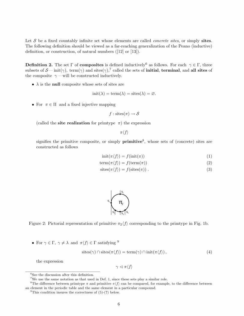
Figure 1: (a) Pictorially, it is convenient to represent primtypes as spheres with the initial a-sites asmarked points on its upper part, and the terminal a-sites as marked points on its lower part. Thus,the sites in init(π) ∩ term(π) are points on the equator. (b) To simplify subsequent drawings, wereplace the spheres by circles and the equator reduces to two, left and right, points.

For every primtype π we introduce the set of all a-sites

sites(π) = init(π) ∪ term(π) .

5

Let S be a fixed countably infinite set whose elements are called concrete sites, or simply sites.The following definition should be viewed as a far-reaching generalization of the Peano (inductive)definition, or construction, of natural numbers ([12] or [13]).

Definition 2. The set Γ of composites is defined inductively6 as follows. For each γ ∈ Γ, threesubsets of S— init(γ), term(γ) and sites(γ),7 called the sets of initial, terminal, and all sites ofthe composite γ —will be constructed inductively.

• λ is the null composite whose sets of sites are

init(λ) = term(λ) = sites(λ) = ∅.

• For π ∈ Π and a fixed injective mapping

f : sites(π) → S

(called the site realization for primtype π) the expression

π〈f〉

signifies the primitive composite, or simply primitive8, whose sets of (concrete) sites areconstructed as follows

init(π〈f〉) = f(init(π)) (1)term(π〈f〉) = f(term(π)) (2)sites(π〈f〉) = f(sites(π)) . (3)

π2

s1

s2

s4s5s3

Figure 2: Pictorial representation of primitive π2〈f〉 corresponding to the primtype in Fig. 1b.

• For γ ∈ Γ, γ 6= λ and π〈f〉 ∈ Γ satisfying 9

sites(γ) ∩ sites(π〈f〉) = term(γ) ∩ init(π〈f〉) , (4)

the expressionγ C π〈f〉

6See the discussion after this definition.7We use the same notation as that used in Def. 1, since these sets play a similar role.8The difference between primtype π and primitive π〈f〉 can be compared, for example, to the difference between

an element in the periodic table and the same element in a particular compound.9This condition insures the correctness of (5)-(7) below.

6

signifies the composite γ′, whose sets of (concrete) sites are constructed as follows

init(γ′) = init(γ) ∪ [init(π〈f〉) \ term(γ)] (5)term(γ′) = [term(γ) \ init(π〈f〉)] ∪ term(π〈f〉) (6)sites(γ′) = sites(γ) ∪ sites(π〈f〉). (7)

We will call γ′ the composite obtained from γ by attachment of primitive π〈f〉, wherethe “attachment” means attaching to each other the identical sites in term(γ) and init(π〈f〉).

Thus, every composite γ is specified by the following inductive expression encapsulating itsconstruction process

γ = π1〈f1〉 C π2〈f2〉 C . . . C πn〈fn〉.(See Fig. 3, 4, 5.) We will assume that the above expression is valid for n = 0 and in this casedenotes λ. I

For a composite γ, the setcont(γ) = init(γ) ∩ term(γ) (8)

will be called the set of continuation sites.

π5

s2

s4

π4s3

π3

s1

s2 s3

γ

s4 s3

s1s2 s3s4

s5 s6 s7 s8

s5 s6

s7

s8

Figure 3: A simplified (left) and a detailed pictorial representation of composite γ = π3〈f3〉 Cπ5〈f5〉 C π4〈f4〉 with two continuation sites.

It is important to note that, conceptually, we view the set Γ not as derivative with respectto the set of natural numbers, but rather as a more basic set. In particular, we view the set ofnatural numbers as a very special case of Γ. Consequently, to achieve a necessary degree of rigor, weshould rely on the appropriate generalization of Peano axioms (for natural numbers [12]), includingthe generalization of the induction axiom (see Def. 19). In this paper, however, to retain both areasonable degree of rigor and accessibility of the exposition, we will adapt the following inductiveschemes.

7

π8

s4

s5

s6

π6

s1

π7

s2

Figure 4: Pictorial representation of a “decoupled” composite β = π6〈f6〉 C π7〈f7〉 C π8〈f8〉.

Under the inductive proof of a statement A(γ) about composites, or proof by inductionon γ, we mean the following proof scheme.

• Prove that A(λ) is true.

• For all π〈f〉 prove that A(π〈f〉) is true.

• If A(α) is true and γ = α C π〈f〉, prove that A(γ) is true.

Under the inductive definition, or construction, of objects B(γ) for composites γ ∈ Γ, wemean the following definition (construction) scheme.

• Construct B(λ).

• For any π〈f〉 construct B(π〈f〉).• Assume that B(α) has been constructed and that γ = α C π〈f〉, then construct B(γ).

Note that for a composite γ, the union of its initial and terminal sites could now be smallerthan the set of all sites. Therefore, for a composite γ, it will also be useful to define the set of itsexternal and internal sites

ext(γ) = init(γ) ∪ term(γ)int(γ) = sites(γ) \ ext(γ) .

(9)

It is quite possible that the fuzzy boundary between the “living” and “non-living” objects can beunderstood in terms of the assymptotic growth rate of the size of set ext(γ) during the (generative)process of object “development” 10: normally, the faster the growth rate of | ext(γ)| during the“generation” of object γ, the more complex γ is.

10See section 3.6.

8

π9

s3

π10s3

s1

s2

π11

s3

s5s4

s7

s6

Figure 5: Pictorial representation of composite γ = π9〈f9〉 C π10〈f10〉 C π11〈f11〉 with one contin-uation (s2) and one internal (s3) sites.

Definition 3. For γ ∈ Γ and any injective mapping

h : sites(γ) → S ,

called site replacement, the composite γ〈h〉 is defined inductively as follows.

• λ〈h〉 def= λ

• If γ = π〈f〉, then γ〈h〉 def= π〈g〉, where g = h f .

• Assume that α〈h′〉 has been constructed for any site replacement h′ : sites(α) → S andγ = α C π〈f〉, then

γ〈h〉 def= α〈h′〉 C π〈g〉 ,where h′ = h

∣∣sites(α)

and g is as above.

I

Lemma 1. For γ ∈ Γ and any site replacement h : sites(γ) → S, Def. 3 correctly defines compositeγ〈h〉, and, moreover, the following useful relationships are true

init(γ〈h〉) = h(init(γ))term(γ〈h〉) = h(term(γ))sites(γ〈h〉) = h(sites(γ)) .

(10)

Proof.The proof is by induction on γ.

• By Def. 3, λ〈h〉 = λ, hence all the sets in (10) are empty and the equalities hold.

9

• Let γ = π〈f〉 and h : sites(γ) → S be a site replacement. By (3), f(sites(π)) = sites(γ) andh f : sites(π) → S is an injective mapping. By Def. 2, γ〈h〉 = π〈h f 〉 is defined correctly.Next, according to (1–3)

init(π〈f〉) = f(init(π))term(π〈f〉) = f(term(π))sites(π〈f〉) = f(sites(π))

and

init(π〈h f 〉) = (h f)(init(π)) = h(f(init(π))

)

term(π〈h f 〉) = (h f)(term(π)) = h(f(term(π))

)

sites(π〈h f 〉) = (h f)(sites(π)) = h(f(sites(π))

).

From the last equations we obtain (10):

init(π〈h f 〉) = h(init(π〈f〉))term(π〈h f 〉) = h(term(π〈f〉))sites(π〈h f 〉) = h(sites(π〈f〉)) .

(∗)

• Suppose that for α ∈ Γ the following statement is true: for any site replacement h′ : sites(α) →S the composite α〈h′〉 has been correctly defined and

init(α〈h′〉) = h′(init(α))term(α〈h′〉) = h′(term(α))sites(α〈h′〉) = h′(sites(α)) .

(∗∗)

Let γ = α C π〈f〉 and h : sites(γ) → S be a site replacement. It follows from (7) thatsites(γ) = sites(α) ∪ sites(π〈f〉). Take h′ = h

∣∣sites(α)

. We want to verify (4) for α〈h′〉 andπ〈h f 〉 in order to check the existence of the composite γ〈h〉 = α〈h′〉 C π〈h f 〉.

sites(α〈h′〉) ∩ sites(π〈h f 〉) (∗),(∗∗)=

h′(sites(α)) ∩ h(sites(π〈f〉)) =h (sites(α)) ∩ h(sites(π〈f〉)) =

h [sites(α) ∩ sites(π〈f〉)] (4)=

h [term(α) ∩ init(π〈f〉)] =h [term(α)] ∩ h[init(π〈f〉)] =

h′(term(α)) ∩ h(init(π〈f〉)) (∗),(∗∗)=

term(α〈h′〉) ∩ init(π〈h f 〉) .

Finally, we check (10) for γ〈h〉:

init(γ〈h〉) (5)=

init(α〈h′〉) ∪ [init(π〈h f 〉) \ term(α〈h′〉)] (∗),(∗∗)=

h′(init(α)) ∪ [h(init(π〈f〉)) \ h′(term(α))] =h (init(α)) ∪ [h(init(π〈f〉)) \ h (term(α))] =

h [init(α) ∪ (init(π〈f〉) \ term(α))](5)=

h [init(α C π〈f〉)] =h (init(γ)) .

10

The proof of the equalities

term(γ〈h〉) = h(term(γ))sites(γ〈h〉) = h(sites(γ))

is similar.

¥

Lemma 2. Let γ be a composite, and h1 : sites(γ) → S, h2 : sites(γ〈h1〉) → S be site replacements.Then,

(γ〈h1〉)〈h2〉 = γ〈h2 h1〉.Proof.

The proof is by induction on γ.

• By Def. 3, (λ〈h1〉)〈h2〉 = λ〈h2〉 = λ = λ〈h2 h1〉.• Let γ = π〈f〉. Then,

(γ〈h1〉)〈h2〉 D.3= (π〈h1 f 〉)〈h2〉 D.3= π〈h2 (h1 f)〉 = π〈(h2 h1) f 〉 D.3= π〈f〉〈h2 h1〉.

• Suppose that for α ∈ Γ the following statement is true: for all site replacements g1 :sites(α) → S, g2 : sites(α〈g1〉) → S,

(α〈g1〉)〈g2〉 = α.〈g2 g1.〉 (∗)

Let γ = α C π〈f〉, and h1 : sites(γ) → S, h2 : sites(γ〈h1〉) → S be site replacements. Let

g1 = h1

∣∣sites(α)

, h = h2 h1, g = h2 g1 = h∣∣sites(α)

.

Then,

(γ〈h1〉)〈h2〉 D.3= (α〈g1〉 C π〈h1 f 〉)〈h2〉 D.3= (α〈g1〉)〈h2〉 C π〈h2 h1 f 〉 (∗)=

α〈h2 g1〉 C π 〈h2 h1 f 〉 = α〈g〉 C π〈h f 〉 D.3= γ〈h〉.

¥

Lemma 3. Let γ′ = γ〈h〉. Then, there exists site replacement h′ : sites(γ′) → S such that γ′〈h′〉 = γ.

Proof. By Lemma 1, sites(γ′) = h(sites(γ)). Since h is an injective mapping, let h′ = h−1,h′ : sites(γ′) → S. Then,

(γ〈h〉)〈h′〉 L.2= γ〈h′ h〉 = γ〈idsites(γ)〉 D.3= γ.

¥

11

Definition 4. Two composites α and β will be called similar and denoted as α ≈ β, if there existssite replacement h : sites(β) → S such that

h∣∣ext(β)

= id

andα = β〈h〉.

I

Thus, two composites are similar, if one of them can be obtained from the other by relabelingits internal sites. The basic relationships between the sites of two similar composites are given next.

Lemma 4. If α and β are two similar composites and h is the corresponding site replacement, then

init(α) = init(β), term(α) = term(β), int(α) = h(int(β)).

Proof. By Lemma 3,

init(α) = h(init(β))term(α) = h(term(β))sites(α) = h(sites(β)).

Therefore, it follows from (9) thatint(α) = h(int(β)).

Again from (9), since h∣∣ext(β)

= id ,

init(α) = init(β)term(α) = term(β).

¥

How do we construct new composites out of the old ones? The following definition introducesthe relevant operation of composition of two composites.

Definition 5. Let α and β be two composites satisfying

sites(α) ∩ sites(β) = term(α) ∩ init(β) . (11)

The composition of the above two composites,

α C β ,

is defined by induction on β as follows.

• α C λdef= α

•α C π〈f〉 def=

π〈f〉, α = λα C π〈f〉, α 6= λ (see Def. 2)

12

• Assume that α C γ has been constructed and that β = γ C π〈f〉, then

α C βdef= (α C γ) C π〈f〉.

I

Lemma 5. The sets of sites for the composition of two composites α and β are

init(α C β) = init(α) ∪ [init(β) \ term(α)]term(α C β) = [term(α) \ init(β)] ∪ term(β)sites(α C β) = sites(α) ∪ sites(β)cont(α C β) = [cont(α) ∩ cont(β)] ∪ [cont(α) \ sites(β)] ∪ [cont(β) \ sites(α)].

With respect to definition of the continuation sites (8) one should note that these sites are theonly ones that allow the “continuation” of external sites during the composition.

Lemma 6. Composition is associative, i.e. if α, β, γ are composites such that compositions α C βand (α C β) C γ exist, then the compositions β C γ and α C (β C γ) also exist and

(α C β) C γ = α C (β C γ) .

2.2 Semantic relations, istructs, and parallel composition

As it often happens in science, the accumulated (mainly experimentally) knowledge in a par-ticular domain strongly suggests the “indistinguishability” of some objects or their parts in thefollowing sense: if the corresponding two parts in the object representation are interchanged, novisible/detectable differences in the “behaviour” of the reference physical objects are observed. Itis for this reason that we, as always, need the following concept.

Definition 6. Let α, β be two composites such that

init(α) = init(β), term(α) = term(β).

The expressionα ≡ β

is called semantic identity and signifies the indistinguishability of the corresponding two partsin an object representation (Fig 6). I

Definition 7. Let I be a specified set of semantic identities.11 This set induces naturally thesemantic equivalence relation, or simply semantic relation, denoted ∼ , on the set of compositesΓ as follows.

11Note that, usually, I is a relatively small set.

13

π s2

s1

π s3s2

≡π s2

π s3s2

13

19

14

12

s4

5

s1 s4

s

5s6

s s7s7s8s8 s6

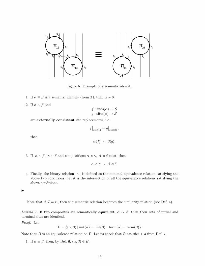
Figure 6: Example of a semantic identity.

1. If α ≡ β is a semantic identity (from I), then α ∼ β.

2. If α ∼ β andf : sites(α) → Sg : sites(β) → S

are externally consistent site replacements, i.e.

f∣∣ext(α)

= g∣∣ext(β)

,

thenα〈f〉 ∼ β〈g〉.

3. If α ∼ β, γ ∼ δ and compositions α C γ, β C δ exist, then

α C γ ∼ β C δ.

4. Finally, the binary relation ∼ is defined as the minimal equivalence relation satisfying theabove two conditions, i.e. it is the intersection of all the equivalence relations satisfying theabove conditions.

I

Note that if I = ∅, then the semantic relation becomes the similarity relation (see Def. 4).

Lemma 7. If two composites are semantically equivalent, α ∼ β, then their sets of initial andterminal sites are identical.

Proof. LetB = (α, β) | init(α) = init(β), term(α) = term(β).

Note that B is an equivalence relation on Γ. Let us check that B satisfies 1–3 from Def. 7.

1. If α ≡ β, then, by Def. 6, (α, β) ∈ B.

14

2. If (α, β) ∈ B and f, g are the corresponding externally consistent site replacements, then

init(α〈f〉) L.1= f(init(α))(9)= f

∣∣ext(α)

(init(α)) = g∣∣ext(β)

(init(α))(α, β) ∈ B

=

g∣∣ext(β)

(init(β))(9)= g(init(β)) L.1= init(β〈g〉) ,

and, similarly,term(α〈f〉) = term(β〈g〉).

Hence, (α〈f〉, β〈g〉) ∈ B.

3. If (α, β), (γ, δ) ∈ B, and the compositions α C γ, β C δ exist, then

init(α C γ) L.5= init(α) ∪ [init(γ) \ term(α)] =

init(β) ∪ [init(δ) \ term(β)] L.5= init(β C δ).

and, similarly,term(α C γ) = init(β C δ).

Hence, (α C γ, β C δ) ∈ B.

From condition 4 of Def. 7, we have ∼ ⊆ B. ¥

Lemma 8. If α ≈ β, then α ∼ β.

One of the simplest semantic identities specifies the indistinguishability between some of thesites in a primitive.

Definition 8. For primitive π〈f〉 and site replacement h : sites(π〈f〉) → S satisfying

h[init(π〈f〉)] = init(π〈f〉)h[term(π〈f〉)] = term(π〈f〉) ,

the semantic identityπ〈f〉 ≡ π〈h f 〉

will be called the site equivalence identity. We will denote by Eqsite(Π) the set of all possiblesuch identities. I

Judging by our present knowledge in physics, i.e. by the indistinguishability between any twoelementary particles of the same type, the set Eqsite(Π) or its generalization might be of particularimportance in a large number of applications.

It is not difficult to anticipate now that, as always is the case, the set of equivalent compositesshould be considered as representing the same physical object.

15

Definition 9. Let Π, I be specified sets of primtypes and semantic identities. The quotient set

Θ = Γ/∼ = [γ] | γ ∈ Γ will be called the set of instance structs, or simply istructs (for (Π, I)). Istruct [λ] will be calledthe empty istruct and denoted λ. For each istruct [γ], also denoted, γ the three sets of sites aredefined as follows

init(γ) = init(γ), term(γ) = term(γ), ext(γ) = ext(γ) .

INote that the correctness of the last definition follows from Lemma 7.

The concept of quotient set plays an important role in the proposed representation model: theconcept of istruct should be considered as the first step in the process of connecting the “abstract”representation by means of composites with the “actual” objects.12 In view of this, it mightbe useful to remember how to work with quotient sets. Some of the most known examples ofequivalence relations are rational numbers (1/2 ∼ 2/4 ∼ . . .) and systems of (linear) equations(systems are equivalent, iff they have the same solutions). So, in order to work with the quotientset, one should be able, first, to find (algorithmically) a “canonical” element of the equivalenceclass (which represents the class), and, second, learn how to operate with the original set (add,multiply, and, in our case, attach or replace sites). Note that, although the general problem offinding a canonical composite is undecidable, in each application of the proposed model one shouldmake sure that there is an efficient algorithm for finding the canonical composite for any istruct.

Definition 10. For an istruct γ and an injective mapping h : ext(γ) → S , called istruct sitereplacement, the istruct γ〈h〉 is defined as

γ〈h〉 = [γ〈h〉] ,

where γ ∈ γ and h : sites(γ) → S is a site replacement satisfying

h∣∣ext(γ)

= h.

INote that although a composite, typically, has internal sites, we do not introduce the concept

of internal sites for an istruct, since an istruct is “independent” of the labels of the internal sitesin its canonical composite. Also, as was the case with composites, in general, we cannot arbitrarilymodify the labels of the external sites of an istruct, since the modification may change the mannerof attachment of this istruct to other istructs.

Lemma 9. For an istruct γ and an injective mapping h : ext(γ) → S , the istruct γ〈h〉 iscorrectly defined in Def. 10, i.e. it does not depend on the choice of γ and h.Proof. Let γ1, γ2 ∈ γ, and h1 : sites(γ1) → S, h2 : sites(γ2) → S be site replacements satisfying

h1

∣∣ext(γ1)

= h2

∣∣ext(γ2)

= h,

i.e. h1 and h2 are externally consistent. By Def. 9, γ1 ∼ γ2. Therefore, according to Def. 7.2,γ1〈h1〉 ∼ γ2〈h2〉. ¥

12For the next step, see the concept of struct introduced in Def. 21.

16

Lemma 10. Let γ be a composite, and h1 : ext(γ) → S, h2 : ext(γ〈h1〉) → S be site replacements.Then,

(γ〈h1〉)〈h2〉 = γ〈h2 h1〉.Proof. Take any γ ∈ γ, h1 : sites(γ) → S, h2 : sites(γ〈h1〉) → S satisfying

h1

∣∣ext( )

= h1, h2

∣∣ext ( 〈h1 〉) = h2.

Then,(γ〈h1〉)〈h2〉 D.10= [(γ〈h1〉)〈h2〉] L.2= [γ〈h2 h1〉] D.10= γ〈h2 h1〉.

¥

Lemma 11. Let γ ′ = γ〈h〉. Then, there exists site replacement h′ : ext(γ ′) → S such thatγ ′〈h′〉 = γ.

Proof. The proof of this lemma is similar to that of Lemma 3. ¥

Lemma 12. If α〈h〉 = β〈h〉, then α = β.

Lemma 13. Let S ′ ⊆ S be a finite subset of the set of sites. Let γ be an istruct, and αi∞i=1 be asequence of istructs, hi∞i=1 be a sequence of site replacements such that for all i ∈ Z+,

• ext(αi) ⊆ S ′

• γ = αi〈hi〉.Then there exist indices i 6= j such that αi = αj .

Proof. For each i ∈ Z+, the domain of hi is a subset of S ′ and the image of hi is equal to ext(γ).Both, S ′ and ext(γ) are finite sets. Therefore, there exist indices i 6= j, such that hi = hj , and, byLemma 12, we have αi = αj . ¥

As we did for the composites, we now introduce the concept of composition for istructs.

Definition 11. Let α, β be two istructs satisfying

ext(α) ∩ ext(β) = term(α) ∩ init(β) .

The composition of the above two istructs, α C β , is defined as

α C β = [α C β] ,

whereα ∈ α, β ∈ β, and α C β exists.

I

Lemma 14. The composition of the above istructs α and β is correctly defined, i.e. it does notdepend on the choice of α and β, and exists.

17

Proof. To prove the existence, we need to find γ ∈ α and δ ∈ β, such that γ C δ exists. Take anyα ∈ α, β ∈ β. There exist site replacements

f : sites(α) → S, g : sites(β) → Ssatisfying

f∣∣ext(α)

= id, g∣∣ext(β)

= id

andint(α〈f〉) ∩ sites(β〈g〉) = ∅int(β〈g〉) ∩ sites(α〈f〉) = ∅.

(∗)

Note that by Def. 7,α〈f〉 ∼ α and β〈g〉 ∼ β, or,

α〈f〉 ∈ α and β〈g〉 ∈ β. (∗∗)Therefore,

sites(α〈f〉) ∩ sites(β〈g〉) (9)=

[ext(α〈f〉) ∪ int(α〈f〉)] ∩ [ext(β〈g〉) ∪ int(β〈g〉)] (∗)=

ext(α〈f〉) ∩ ext(β〈g〉) (∗∗)= ext(α) ∩ ext(β) Def.11=

term(α) ∩ init(β)(∗∗)= term(α〈f〉) ∩ init(β〈g〉),

and it follows from (4) that the composition α〈f〉 C β〈g〉 exists.

If α ∼ α′, β ∼ β′, then by Def. 7

α C β ∼ α′ C β′ ,

and so α C β does not depend on the choice of α and β, i.e. the correctness of Def. 11 is proved.¥

Lemma 15. Composition of istructs is associative.

The next two definitions single out a certain subclass of compositions that can be thought ofas representing “independent”, or “parallel”, attachment of composites.

Definition 12. For α, β ∈ Γ, for which

sites(α) ∩ sites(β) = cont(α) ∩ cont(β) , (12)

the composite α C β will be denoted asα ‖β

and called the parallel composition of α and β. I

Lemma 16. The above definition is correct, i.e. from (12) it follows that parallel compositions α ‖βand β ‖α exist. Moreover,

init(α ‖β) = init(α) ∪ init(β)term(α ‖β) = term(α) ∪ term(β)cont(α ‖β) = cont(α) ∪ cont(β).

(13)

18

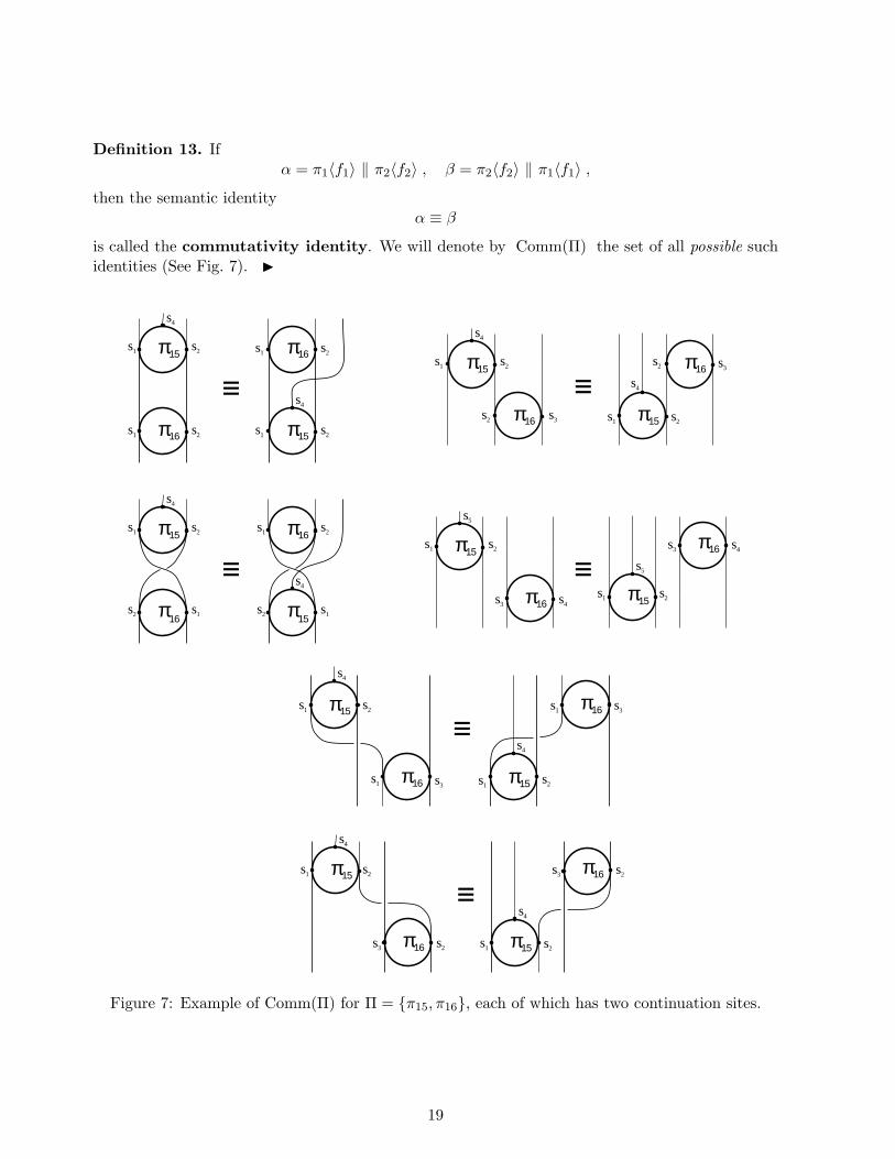
Definition 13. Ifα = π1〈f1〉 ‖ π2〈f2〉 , β = π2〈f2〉 ‖ π1〈f1〉 ,

then the semantic identityα ≡ β

is called the commutativity identity. We will denote by Comm(Π) the set of all possible suchidentities (See Fig. 7). I

s2s1

s3s2

≡s2s1

s3s2

π16

π15

π15

π16

s2

s1s2s3

≡π16

π15

s2

s2s3 π16

π15

s1

s2

s1s3s1

≡π16

π15

s2

s3s1 π16

π15

s1

s2s1

≡π15

s2s1 π16

s2s1 π16

s2s1 π15

s2s1

≡π15

s1s2 π16

s2s1 π16

s1s2 π15

s2s1

s4s3

≡π16

π15

s2s1

s4s3 π16

π15

s4

s4

s4

s4

s4

s4

s5

s5

s4

s4

s4

s4

Figure 7: Example of Comm(Π) for Π = π15, π16, each of which has two continuation sites.

19

Lemma 17. Let I ⊇ Comm(Π). If for composites α, β the parallel composition α ‖β exists, then

α ‖β ∼ β ‖α.

Lemma 18. Let I = Comm(Π) and B be the set of all bijections b : [1, n] → [1, n] . If γ =π1〈f1〉 ‖ . . . ‖πn〈fn〉, then int(γ) = ∅ and

γ =

πb(1)〈fb(1)〉 ‖ . . . ‖ πb(n)〈fb(n)〉∣∣ b ∈ B

.

2.3 Itransformations

In this section, we make the next big step by introducing the next central concept, the concept ofistruct transformation, i.e. the concept of istruct “operation”.

Definition 14. Let (Π, I) be given and let Θ be the corresponding set of istructs. A pair τ =(α,β) of istructs such that there exists istruct δ satisfying

β = α C δ ,

will be called an instance transformation, or simply itransformation, α will be called thecontext of itransformation τ , and

ext(τ ) def= ext(α) ∪ ext(β).

If α = [λ], the itransformation will be called context free. The set of all itransformations for(Π, I) will be denoted by T (See Fig. 8). I

s3s2

s4s3

s2s1 π18

π17

s5

π17

α

δ

β

Figure 8: Pictorial represenatation of itransformation τ = ( [ π17〈f17〉 ], [π17〈f17〉 C π17〈g17〉 Cπ18〈f18〉 ] ). The shaded composite π17〈f17〉 is an element from the context [π17〈f17〉].

As was the case with composites and istructs, it is useful to introduce the concept of itransfor-mation site replacement.

20

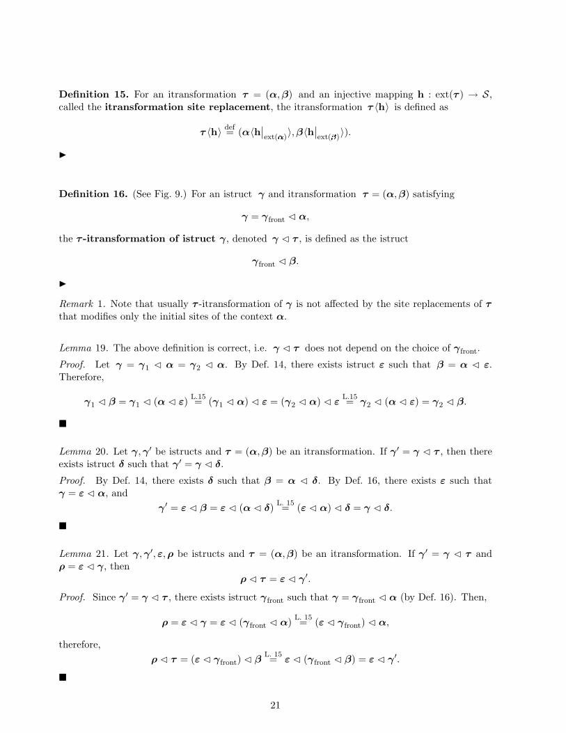
Definition 15. For an itransformation τ = (α,β) and an injective mapping h : ext(τ ) → S,called the itransformation site replacement, the itransformation τ 〈h〉 is defined as

τ 〈h〉 def= (α〈h∣∣ext()

〉, β〈h∣∣ext()

〉).

I

Definition 16. (See Fig. 9.) For an istruct γ and itransformation τ = (α,β) satisfying

γ = γfront C α,

the τ -itransformation of istruct γ, denoted γ C τ , is defined as the istruct

γfront C β.

I

Remark 1. Note that usually τ -itransformation of γ is not affected by the site replacements of τthat modifies only the initial sites of the context α.

Lemma 19. The above definition is correct, i.e. γ C τ does not depend on the choice of γfront.

Proof. Let γ = γ1 C α = γ2 C α. By Def. 14, there exists istruct ε such that β = α C ε.Therefore,

γ1 C β = γ1 C (α C ε) L.15= (γ1 C α) C ε = (γ2 C α) C εL.15= γ2 C (α C ε) = γ2 C β.

¥

Lemma 20. Let γ, γ ′ be istructs and τ = (α, β) be an itransformation. If γ ′ = γ C τ , then thereexists istruct δ such that γ ′ = γ C δ.

Proof. By Def. 14, there exists δ such that β = α C δ. By Def. 16, there exists ε such thatγ = ε C α, and

γ ′ = ε C β = ε C (α C δ) L. 15= (ε C α) C δ = γ C δ.

¥

Lemma 21. Let γ, γ ′, ε, ρ be istructs and τ = (α,β) be an itransformation. If γ ′ = γ C τ andρ = ε C γ, then

ρ C τ = ε C γ ′.

Proof. Since γ ′ = γ C τ , there exists istruct γfront such that γ = γfront C α (by Def. 16). Then,

ρ = ε C γ = ε C (γfront C α) L. 15= (ε C γfront) C α,

therefore,ρ C τ = (ε C γfront) C β

L. 15= ε C (γfront C β) = ε C γ ′.

¥

21

According to the above definition, the action of an itransformation τ can be viewed as an“attachment” of τ to some istruct which contains the corresponding context. Thus, one can thinkof an istruct as of a representation of the object’s constructive history (via the history of applieditransformations). To put it more precisely, an istruct represents all possible indistinguishableconstruction pathways for a given object. An itransformation context is a part of the istruct, itrepresents a part of the object’s constructive history. The itransformation does not “delete” anyinformation from the istruct, and therefore it can be thought of as an evolutionary transformation.

One should also emphasize some basic distinctions (of transformations) from Chomsky produc-tion rules.

• Although the context of a Chomsky production rule (regardless of whether it is a context-free,context-sensitive or unrestricted production) is a part of the string, since the string does notcapture its constructive history, the production cannot refer to the corresponding part of thehistory.

• When a production is applied, the non-terminal symbol, which served as the productioncontext, is erased, and cannot serve as a context for further productions. Therefore, inChomsky’s model, productions erase the string’s evolutionary history.

It is interesting to note that in [23] Chomsky speaks of certain grammatical rules which can beapplied to sentences only if we “. . . know not only the final shape of these sentences but also their‘history of derivation’.” He does not offer, however, any formal definition of such rules.

s2s1

s4s2

s1s6

π17

π17

π18

s2s1 π18

s2s1 π17

s3

s1 π18

τs2

s3

s5

α

γfront

γfront

β

Figure 9: Example of τ -itransformation (from Fig. 8) of istruct γ = [π18〈g18〉 C π17〈f17〉]. Theshaded parts in the representative composites correspond to the context of τ .

Definition 17. If γ, γ ′ ∈ Θ, τ = (α, β) ∈ T , and there exists a site replacement h such that

γ ′ = γ C τ 〈h〉,then we will signify it

γ→ γ ′ .

I

22

As in the classical case (for which we recommend [24] ), to formulate the axiom of induction weneed an auxiliary definition.

Definition 18. The set of immediate ancestors of an istruct γ is defined as

AI(γ) def= α ∈ Θ | (α 6= γ) and (∃ τ ∈ T α→ γ) .

I

Definition 19. (Induction axiom for istructs.) If Θ′ is a subset of Θ satisfying the followingconditions

• λ ∈ Θ′

• ∀γ ∈ Θ [AI(γ) ⊆ Θ′ =⇒ γ ∈ Θ′ ] ,

then Θ′ = Θ. I

This axiom is necessary whenever a proof or definition by induction on istructs is required.We are ready now to introduce our underlying, or basic, mathematical structure.

Definition 20. Let Π be a finite set of primtypes, I be a specified set of semantic identities, andΘ, T be the corresponding sets of istructs and itransformations. If the induction axiom for istructsholds, we will call (Π, I) an inductive structure. I

2.4 The string inductive structure

In this and the following examples, function f : [1, n] → Z+ will be specified by the list of its valuesf(1), . . . , f(n). Also, for simplicity, we will use the same notation if f : a1, a2, . . . , an → Z+,where the domain of f is a finite subset of set A of abstract sites (see Def. 1).

Example 1. Let Σ = a, b, . . . , z be a finite alphabet. Consider a set of primtypes Π =πa, πb, . . . , πz indexed by the elements of Σ. Let the set A of a-sites be a1, a2, a3, and foreach π ∈ Π,

init(π) = a1term(π) = a2, a3.

The set S of sites is N. Then, each composite corresponds to a string or to a finite set of strings 13

over Σ. E.g., both composites πa〈1, 2, 3〉 C πb〈3, 4, 5〉 and πb〈1, 3, 5〉 C πa〈3, 2, 4〉 correspond to thesame string ab. However, each composite represents different “construction path” for this string:the first composite corresponds to the concatenation of letter b after a, and the second one, to theconcatenation of a in front of b.

To model ”strings”, we would like to model the situation where these construction paths areequivalent. To this end, let us, for each α, β ∈ Σ, denote by idαβ the following semantic identity:

πα〈1, 2, 3〉 C πβ 〈3, 4, 5〉 ≡ πβ 〈1, 3, 5〉 C πα〈3, 2, 4〉.13This is the case when the composite is “decoupled” (see Fig. 4).

23

LetI = Comm(Π) ∪ idαβ | α, β ∈ Σ.

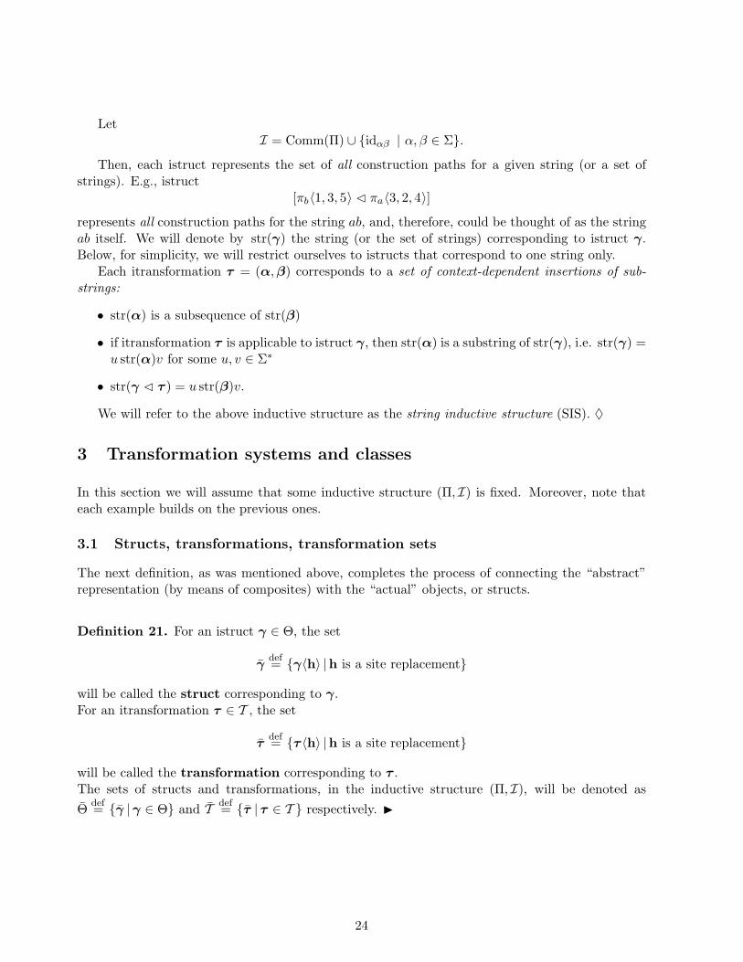
Then, each istruct represents the set of all construction paths for a given string (or a set ofstrings). E.g., istruct

[πb〈1, 3, 5〉 C πa〈3, 2, 4〉]represents all construction paths for the string ab, and, therefore, could be thought of as the stringab itself. We will denote by str(γ) the string (or the set of strings) corresponding to istruct γ.Below, for simplicity, we will restrict ourselves to istructs that correspond to one string only.

Each itransformation τ = (α, β) corresponds to a set of context-dependent insertions of sub-strings:

• str(α) is a subsequence of str(β)

• if itransformation τ is applicable to istruct γ, then str(α) is a substring of str(γ), i.e. str(γ) =u str(α)v for some u, v ∈ Σ∗

• str(γ C τ ) = u str(β)v.

We will refer to the above inductive structure as the string inductive structure (SIS). ♦

3 Transformation systems and classes

In this section we will assume that some inductive structure (Π, I) is fixed. Moreover, note thateach example builds on the previous ones.

3.1 Structs, transformations, transformation sets

The next definition, as was mentioned above, completes the process of connecting the “abstract”representation (by means of composites) with the “actual” objects, or structs.

Definition 21. For an istruct γ ∈ Θ, the set

γdef= γ〈h〉 |h is a site replacement

will be called the struct corresponding to γ.For an itransformation τ ∈ T , the set

τdef= τ 〈h〉 |h is a site replacement

will be called the transformation corresponding to τ .The sets of structs and transformations, in the inductive structure (Π, I), will be denoted asΘ def= γ |γ ∈ Θ and T def= τ | τ ∈ T respectively. I

24

Example 2. For each string u ∈ Σ∗, there are infinitely many istructs in the string inductivestructure of Example 1 corresponding to u. E.g., if u = ab, then istructs

πa〈1, 2, 3〉 C πb〈3, 4, 5〉πa〈2, 3, 4〉 C πb〈4, 5, 6〉

etc.

differing only in site labels, correspond to u.However, for each string u ∈ Σ∗, there exists unique struct γu corresponding to it, which, for

convenience, we will denote identically (γu = u).Similarly, every set of context-dependent insertion operations uniquely corresponds to a trans-

formation. The transformation which corresponds to the insertion of string v between strings uand w will be denoted as uw → uvw. ♦

Lemma 22. Let α, β be two istructs and let h : ext(α) → S be a site replacement such thatβ = α〈h〉. Then α = β.

Proof. Let γ ∈ β. Then γ = β〈f〉 for some site replacement f : ext(β) → S. According toLemma 10,

γ = (α〈h〉)〈f〉 = α〈f h〉 ∈ α.

Therefore, β ⊆ α.By Lemma 11, there exists site replacement h′ : ext(β) → S such that α = β〈h′〉, so we have

α ⊆ β .Hence, α = β. ¥

Definition 22. A finite set of transformations T ⊂ T will be called a transformation set. I

As was mentioned above and as can be seen from the above example, it is structs that encodethe real-world objects, since, if we used istructs or composites for this purpose, we would have hadinfinitely many encodings of the same object. However, now, having adopted this interpretation,we are faced with the situation in which it is impossible to define the action of a transformation ona struct. We address this problem by introducing, in the next section, the concepts of ipaths andpaths induced by a transformation set. We will then define,in the following sections, operations ofcomposition and embedding on paths via ipaths.

3.2 Ipaths and paths

We first introduce the concept of ipath.

Definition 23. Let T be a transformation set in (Π, I). If α1, α2, . . . ,αn+1 are istructs andτ 1, . . . , τn are itransformations such that τ 1, . . . , τn ∈ T and

αi+1 = αi C τ i, i ∈ [1, n],

then the tuple(α1, τ 1, α2, τ 2, . . . , τn, αn+1)

25

will be called a T -ipath from α1 to αn+1, or simply ipath when no confusion arises. The set ofall T -ipaths will be denoted by IP T .

For an ipath c, begin(c) def= α1, end(c) def= αn+1 will be called the beginning and the end ofipath c, respectively.

The length, |c|, of the above ipath c is defined to be n:

|c| def= n.

I

Definition 24. Ipaths (α1, τ 1, . . . , τm,αm+1), (β1, δ1, . . . , δn, βn+1) ∈ IP T will be called equiv-alent, if m = n and there exist site replacements gi : ext(αi) → S, i ∈ [1, n + 1] andhi : ext(τ j) → S, i ∈ [1, n] such that

βi = αi〈gi〉, i ∈ [1, n + 1]δi = τ i〈hi〉, i ∈ [1, n]

and for i ∈ [1, n]hi

∣∣ext( i)∩ ext(i)

= gi

∣∣ext( i)∩ ext(i)

hi

∣∣ext( i)∩ ext(i+1)

= gi

∣∣ext( i)∩ ext(i+1)

.

We will denote the equivalence of ipaths c1, c2 ∈ IP T as c1 ∼ c2. I

Example 3. In SIS, let T be a transformation set consisting of one transformation τ = (λ, β),where β = [πa〈1, 2, 3〉]. This transformation corresponds to the context-independent insertion ofletter a. Consider two T -ipaths:

c1 = (πa〈1, 2, 3〉, τ 〈2, 4, 5〉, πa〈1, 2, 3〉 C τ 〈2, 4, 5〉)c2 = (πa〈1, 2, 3〉, τ 〈3, 4, 5〉, πa〈1, 2, 3〉 C τ 〈3, 4, 5〉).

These ipaths correspond to the insertions of letter a at the beginning and at the end of string“a”. They are not equivalent. Indeed, assume otherwise, and let h1, g1, h2 be site replacementsthat establish the equivalence. By Def. 24, h1 = id and g1

∣∣2 = h1

∣∣2, which implies that

τ 〈3, 4, 5〉 = τ 〈2, 4, 5〉, contradiction!However, ipath

c3 = (πa〈2, 3, 4〉, τ 〈3, 5, 6〉, πa〈2, 3, 4〉 C τ 〈3, 5, 6〉)is equivalent to c1. The corresponding site replacements are defined as follows:

g1(i) = i + 1, i ∈ 1, 2, 3h1(i) = i + 1, i ∈ 2, 4, 5g2(i) = i + 1, i ∈ 1, 3, 4, 5.

♦

We now introduce the concept of path.

26

Definition 25. For an ipath c, the set

cdef= c′ ∈ IP T | c′ ∼ c

will be called the T -path, or simply path, corresponding to c.For a path c, begin(c) def= begin(c) and end(c) def= end(c) will be called the beginning and the

end of path c, respectively; |c| def= |c| is the length of path c.For n ≥ 0, Pn

T will denote the set of all paths of length n, and PTdef= ∪∞n=0P

nT will denote the

set of all paths.For α, β ∈ Θ,

PT (α, β) def= p ∈ PT | begin(p) = α, end(p) = βis the set of all paths from α to β. Finally,

PnT (α, β) def= PT (α, β) ∩ Pn

T .

I

Example 4. For the transformation set T from the previous example, there are two different pathsbetween structs a and aa:

PT (a, aa) = c1, c2.♦

Lemma 23. For any path p, begin(p) and end(p) are correctly defined, i.e. they do not depend onthe choice of ipath c ∈ p.

Proof. Letc1 = (α1, τ 1, . . . ,αm+1)c2 = (β1, δ1, . . . , βn+1)

and c1, c2 ∈ p. By Def. 25, c1 ∼ c2. Therefore, by Def. 24, in particular, there exists a sitereplacement h1 : ext(α1) → S such that β1 = α1〈h1〉. According to Lemma 22, β1 = α1, i.e.begin(p) does not depend on the choice of ipath c ∈ p.

Similarly, m = n, and βn+1 = αm+1 . Hence, end(p) does not depend on the choice of c ∈ p.¥

3.3 Path composition

Definition 26. If c1 = (α1, τ 1, . . . , τn,αn+1) and c2 = (αn+1, τn+1, . . . , τn+m, αn+m+1) are T -ipaths, then T -ipath

c2 c1def= (α1, τ 1, . . . , τn+m, αn+m+1)

will be called the composition of c1 and c2.For convenience, we define c2 c1 = c1, if end(c1) 6= begin(c2). I

27

Definition 27. For two paths p1, p2 ∈ PT satisfying end(p1) = begin(p2), the composition of p1

and p2 is defined asp2 p1

def= c,

where c = c2 c1, c1 ∈ p1, c2 ∈ p2, and end(c1) = begin(c2).Again, if end(p1) 6= begin(p2), then p2 p1

def= p1.I

Lemma 24. The composition of paths is defined correctly, i.e. it does not depend on the choice ofipaths c1 and c2.

Proof. Let c1, c2, c′1, c

′2 be ipaths, such that c1 ∼ c′1, c2 ∼ c′2 and

end(c1) = begin(c2)end(c′1) = begin(c′2).

(∗)

We need to show that c2 c1 ∼ c′2 c′1.By Def. 24, for j ∈ 1, 2, we have

cj = (αj1, τ

j1, . . . , α

jnj+1)

c′j = (βj1, δ

j1, . . . ,β

jnj+1),

whereα1

n1= α2

1, β1n1

= β21,

and there exist site replacements

hji : ext(αj

i ) → S, i ∈ [1, nj ]gji : ext(τ j

i ) → S, i ∈ [1, nj ],

such that the conditions in Def. 24 are fulfilled. It follows from (∗) that one can choose thesesite replacements in such a way that h1

n1+1 = h21 and g1

n1= g2

1. Therefore, the following sitereplacements are correctly specified:

hi = h1i , i ∈ [1, n1 + 1]

hi = h2i−n1

, i ∈ [n1 + 1, n1 + 1 + n2]gi = g1

i , i ∈ [1, n1]gi = g2

i−n1, i ∈ [n1 + 1, n1 + n2].

This set of site replacements satisfies the conditions of Def. 24. Hence, c2 c1 ∼ c′2 c′1. ¥

3.4 Elementary paths

In an inductive structure, the set of all “basic” (with respect to T ) paths beginning at a struct γwill play a useful role below.

28

Definition 28. Let, as above, T be a transformation set in inductive structure (Π, I). For a structγ ∈ Θ,

EP T (γ) def=⋃

∈Θ

P 1T (γ, α)

will be called the set of elementary path from γ.For an elementary path c ∈ EP T (γ), where c = (γ, τ , α), the transformation τ ∈ T will be

called the transformation for elementary path c. I

Lemma 25. For all γ ∈ Θ, EP T (γ) is finite.

Proof. Since T is finite, it is sufficient to prove that for every τ ∈ T , the set⋃

′∈Θ

P 1(γ, γ ′)

is finite.Suppose that on the contrary

⋃

′∈Θ

P 1(γ, γ ′) = pi | i ∈ Z+,

where pi 6= pj if i 6= j.Let γ, τ be some fixed elements from γ, τ , respectively.For each i ∈ Z+, choose an ipath ci ∈ pi, ci = (γi, τ i, γ

′i). There exist site replacements

fi : ext(γi) → S, gi : ext(τ i) → S such that γ = γi〈fi〉, τ = τ i〈gi〉.Let hi : ext(γi) → S be a site replacement defined as

hi(s) =

gi(s), s ∈ ext(τ i)fi(s), s 6∈ ext(τ i).

Letδi = γi〈hi〉δ′i = δi C τ .

We have c′i = (δi, τ , δ′i) ∼ ci. Moreover, ext(δi) ⊆ ext(γ) ∪ ext(τ ). By Lemma 13, there existindices i, j, i 6= j, such that δi = δj . Hence, δ′i = δ′j , c′i = c′j and pi = pj , contradiction! ¥

3.5 Path embedding

Since in an inductive structure its T -path are of great importance, in this section, we introduce inthe simplest but important relationship between two path.

Definition 29. For two T -ipaths c1 = (α1, τ 1, . . . , τm, αm+1) and c2 = (β1, δ1, . . . , δm, βm+1),we will say that c1 can be embedded in c2 and denote this fact by c1 → c2, if m = n and thereexists istruct γ such that β1 = γ C α1 and for all i ∈ [1, n], δi = τ i.

A path p1 can be embedded in path p2 (p1 → p2), if there exist ipaths c1 ∈ p1, c2 ∈ p2,such that c1 can be embedded in c2. I

29

Example 5. Continuing Example 3, let two ipath be

c6 = (πa〈2, 4, 5〉, τ 〈4, 6, 7〉, πa〈2, 4, 5〉 C τ 〈4, 6, 7〉)c7 = (πa〈1, 2, 3〉 C τ 〈2, 4, 5〉, τ 〈4, 6, 7〉, πa〈1, 2, 3〉 C τ 〈2, 4, 5〉 C τ 〈4, 6, 7〉).

Then, c6 → c7, and the corresponding γ from Def. 29 is equal to [πa〈1, 2, 3〉].Path c6 corresponds to the insertion of letter a at the beginning of string “a”, and path c7

corresponds to the insertion of letter a in the middle of string “aa”.For ipath

c9 = (πa〈1, 2, 3〉 C τ 〈2, 4, 5〉, τ 〈5, 6, 7〉, πa〈1, 2, 3〉 C τ 〈2, 4, 5〉 C τ 〈5, 6, 7〉),

which represents insertion of a at the end of “aa”, c6 6→ c9, and c6 6→ c9. ♦

Lemma 26. If c1 → c2, then for all i ∈ [1,m + 1], βi = γ C αi.

Proof. By Def. 29, β1 = γ C α1. Let i ∈ [1,m] and βi = γ C αi. Then,

βi+1 = βi C τ i = (γ C αi) C τ iL. 21= γ C (αi C τ i) = γ C αi+1,

and the Lemma is proved by induction on i. ¥

Lemma 27. If p1 → p2, then for all c1 ∈ p1 there exists c2 ∈ p2 such that c1 → c2.

Proof. Let p1 → p2. By Def. 29, there exist ipaths c01 ∈ p1, c0

2 ∈ p2 such that c01 → c0

2.Let

c1 = (α1, τ 1, . . . ,αm+1) ∈ p1

c01 = (α0

1, τ01, . . . ,α

0m0+1)

c02 = (β0

1, τ01, . . . ,β

0m0+1).

Since c1 ∼ c01, m = m0 and, by Def. 24 there exist site replacements gi : ext(α0

i ) → S, hi :ext(τ 0

i ) → S.Let g′i : ext(β0

i ) → S be any site replacements satisfying

g′i∣∣ext(0

i )= gi,

and, for convenience, let h′i = hi. Then

c2 = (β01〈g′1〉, τ 0

1〈h′1〉, . . . ,β0m+1〈g′m+1〉) ∼ c0

2,

and c1 → c2. ¥

3.6 Generating process, typicality measure, and class

As we have seen in the previous sections, a transformation set induces a set of paths betweenstructs. From now on, we will interpret them as struct generation paths and will introduce in thissection the corresponding generating process. For transformation set itself, we introduce a numericparameter for each transformation (which controls the flow of the process in time) and a distinctstruct with which the process starts.

30

Definition 30. A pair WT = (T, l), where T is a transformation set and l : T → R+ is a mapping,will be called a weighted transformation set. Perhaps, the simplest but not neccessesarilythe best interpretation of the transformation weight l(τ ) is the “average time it takes for thetransformation τ ∈ T to be completed”.

A triple TS = (T, l, κ), where (T, l) is a weighted transformation set and κ ∈ Θ is a structcalled the progenitor, will be called a transformation system. I

Definition 31. For a transformation system TS = (T, l, κ), T = τ 1, τ 2, . . . , τm, we will call set

TSdef= γ ∈ Θ |PT (κ, γ) 6= ∅

the set of structs generated by TS. I

Definition 32. Let TS = (T, l, κ) be a transformation system in inductive structure (Π, I), andlet

c = (α1, τ 1, . . . , τn, αn+1) ∈ IP T .

The duration of ipath c (and also of path c) is defined as

l(c) = l(c) def= l(τ 1) + . . . + l(τn).

I

The motivation for the following, one of the central concepts is given right after its definition.In short, for a transformation system, we need the process that actually constructs the structsgenerated by the transformation system. We want to emphasize that we do not insist on thisparticular way of “unfolding” (in time) the information provided by the transformation system, i.e.via the stochastic process, and, in fact, in section Future work are encouraging others to look fordifferent/interesting approaches to the generation of the class elements, not relying on stochasticprocesses.

Definition 33. For a transformation system TS = (T, l, κ), the generating process GTS (orsimply G) is a countable state Markov stochastic process defined as follows:14

1. The states of G are elements of the set TS of structs generated by TS.

2. The amount of time which G spends in state γ is a random variable distributed exponentiallywith mean

L =1∑

p∈EP T ( )

1/l(p). (∗)

3. When G leaves state γ, it chooses randomly an elementary path p ∈ EP T (γ) with probability

L

l(p)(∗∗)

and enters state end(p).14We intentionally use “physical” terminology referring to the “states of the system”.

31

4. All random variables in 2 and 3 are mutually independent.

I

Remark 2. We view the process of struct generation (by a transformation system) as a stochasticprocess, since the choice of the next elementary path and the time it takes is variable (in nature),and, in general, depends not only on the transformation system itself but also on the externalfactors the influence of which cannot be taken into account.

The choice by the process of the next state is modeled based on the following assumptions.First, all elementary paths are indivisible. I.e., an elementary path is either “completed” or not“completed”, since there are no “intermediate” elementary paths. Therefore, the expected amountof time for an elementary path to be completed is independent of the time one has already beenwaiting for the completion of the elementary path. And this property gives us the exponentialdistribution for the amount of time which the process spends in each state. Second, the elements ofEP T (γ) are all, independently of each other and simultaneously, “competing” for the applicationbut only one of them is actually completed first. These two assumptions lead to formulas (∗) and(∗∗).

We assume all random variables to be independent, since we postulate that the choice of thetransformation that is applied to a particular struct and the time of its application depend only onthe struct’s structure. I.e., these random variables depend neither on the path that has lead to thestruct, nor on the time it took to generate the struct.

Definition 34. Let TS be a transformation system and G be the generating process for TS. LetEG(γ) be the expected time spent by G in state γ. We define

EGdef=

∑

∈TS

EG(γ).

If EG is finite, we will say that transformation system TS satisfies the typicality measureexistence condition and we will call such a transformation system a class transformationsystem or simply class. The set of elements of class C will be denoted by C. I

The next definition introduces an important concept of struct typicality with respect to a classC.

Definition 35. Let C be a class and G be the generating process for C. For γ ∈ C, we define

νC(γ) def=EG(γ)

EG.

For γ 6∈ C, νC(γ) def= 0. Measure νC on Θ will be called C-typicality measure, or simply thetypicality. I

Remark 3. For a transformation system TS = (T, l, κ) and a path p ∈ PT , we will use the phrase“process G passes (entire) p” to refer to an intuitively clear random event, and the probabilityof this event is specified uniquely by the process G. Then, the duration of path p is equal to theexpected time the generating process spends on path p under the condition that it passes p.

32

Definition 36. For a class C = TS and path p ∈ PCdef= PTS, the probability of p is defined as

µC(p) def= P (G passes any path p′ into which p can be embedded).

I

Example 6. Continuing Examples 1, 2, consider the following class (specified by its transformationsystem)

C = (aa → aba, ab → acb, ab → adb, (l1, l2, l3), aa),

and let G = GC be the generating process for C.

aa

aba

adbaacba

p1

p2

p3

Figure 10: Elements and paths of class C in Example 2.

Paths of class C reachable by the generating process are shown in Fig. 10 and have the followingprobabilities:

µC(p1) = 1µC(p2) = µC(p2 p1) = 1/l2

1/l2+1/l3

µC(p3) = µC(p3 p1) = 1/l31/l2+1/l3

.

The set of class elements is C = aa, aba, acba, adba. The expected times the generating processspends in each class element are:

EG(aa) = l1EG(aba) = 1

1/l2+1/l3

EG(acba) = EG(adba) = 0.

Therefore,

EG = l1 +1

1/l2 + 1/l3,

andνC(aa) = l1/EG

νC(aba) = 1EG(1/l2+1/l3)

νC(acba) = νC(adba) = 0.

♦

Remark 4. Note that the typicality of each “terminal” class element is always zero.

33

3.7 Extended string inductive structure and the class of strings

In this section we define a new inductive structure—extended string inductive structure (ESIS)—and the class of strings. One should note the differences between the class of strings introduced nextand the string inductive structure (SIS) introduced in Example 1 (section 2.4) . First, elementsof the class of strings correspond to strings only while some structs in SIS correspond to finitesets of strings. The desire to limit oneself to structs which represent single strings only can nowbe realized using context-dependent itransformations. Second, a typicality measure is defined forelements of the string class, and we will show how to compute the typicality of any class element. Weintroduce two new primitives, σ and πx, to construct itransformation contexts and “termination”transformations, which will ensure the existence of the typicality measure. For simplicity, weconsider strings over the alphabet Σ = a, b. It is also important to keep in mind that theinductive structure introduced here is one of the simplest inductive structures for capturing a verypopular but apparently incompletely specified “string” representation.

The set of abstract sites for the new inductive structure is A = a1, a2, a3 and the set ofconcrete sites is S = 0, 1, 2, . . ..

The set of primtypes is ΠESIS = σ, πa, πb, πx (Fig. 11), where

init(σ) = a1 term(σ) = a2init(πx) = a1 term(πx) = a2init(πa) = a1 term(πa) = a2, a3init(πb) = a1 term(πb) = a2, a3.

πaσ πbπx

Figure 11: Primitive types of the ESIS.

The set of semantic identities of the ESIS is IESIS = αij ≡ βij | i, j ∈ Σ (see Fig. 12), where

αij = πi〈1, 2, 3〉 C σ〈2, 4〉 C πj 〈4, 5, 6〉βij = πj 〈1, 5, 2〉 C σ〈2, 4〉 C πi〈4, 6, 3〉.

πa

σ

πb

1

2 3

2

44

5 6

πa

σ

πb

1

5 22

44

6 3

≡

Figure 12: Semantic identities of the ESIS.

34

Since in each identity the lengths of the left- and the right-hand sides are equal, the inductionaxiom holds for the set of istructs Θ in (ΠESIS , IESIS).

As mentioned above, the resulting inductive structure (Π, I) will be called the extended stringinductive structure.

We now define a class C = (T, l, κ) in inductive structure (ΠESIS , IESIS) called the class

of strings. Recalling that for a transformation τ = (α, β) , ext(τ ) def= ext(α) ∪ ext(β), wedefine the transformation set to be T = τ a, τ b, τ x, τ xx (see Fig. 13), where τ i = ([αi], [βi]) fori ∈ a, b, x, xx and

αa = σ〈1, 2〉βa = σ〈1, 2〉 C πa〈2, 5, 6〉 C σ〈5, 3〉 C σ〈6, 4〉

αb = σ〈1, 2〉βb = σ〈1, 2〉 C πb〈2, 5, 6〉 C σ〈5, 3〉 C σ〈6, 4〉

αx = σ〈1, 2〉βx = σ〈1, 2〉 C πx〈2, 3〉

αxx = σ〈1, 2〉 C πx〈3, 4〉βxx = σ〈1, 2〉 C πx〈3, 4〉 C πx〈2, 5〉.

The weights of the transformations are defined as follows

πa

σ

2

1

65

3

6

4

σ2

5

πb

2

65

3

6

4

2

5 π2

2

x

3

π2

2

x

5

π3

x

4

τa τb τx τxx

externalsites:

1,2,3,4 1,2,3,4 1,2,3 1,2,3,4,5

σσ σ

1

σ1

σ

1

σ

Figure 13: Transformations from the transformation set for the class of strings.

l(τ a) = l(τ b) = l(τ x) = 1, l(τ xx) = 0,

and the progenitor is κ = [σ〈1, 2〉].For each string u = a1 . . . an ∈ Σ∗, there is a corresponding class element γu ∈ C (see Fig. 14),

35

where 15

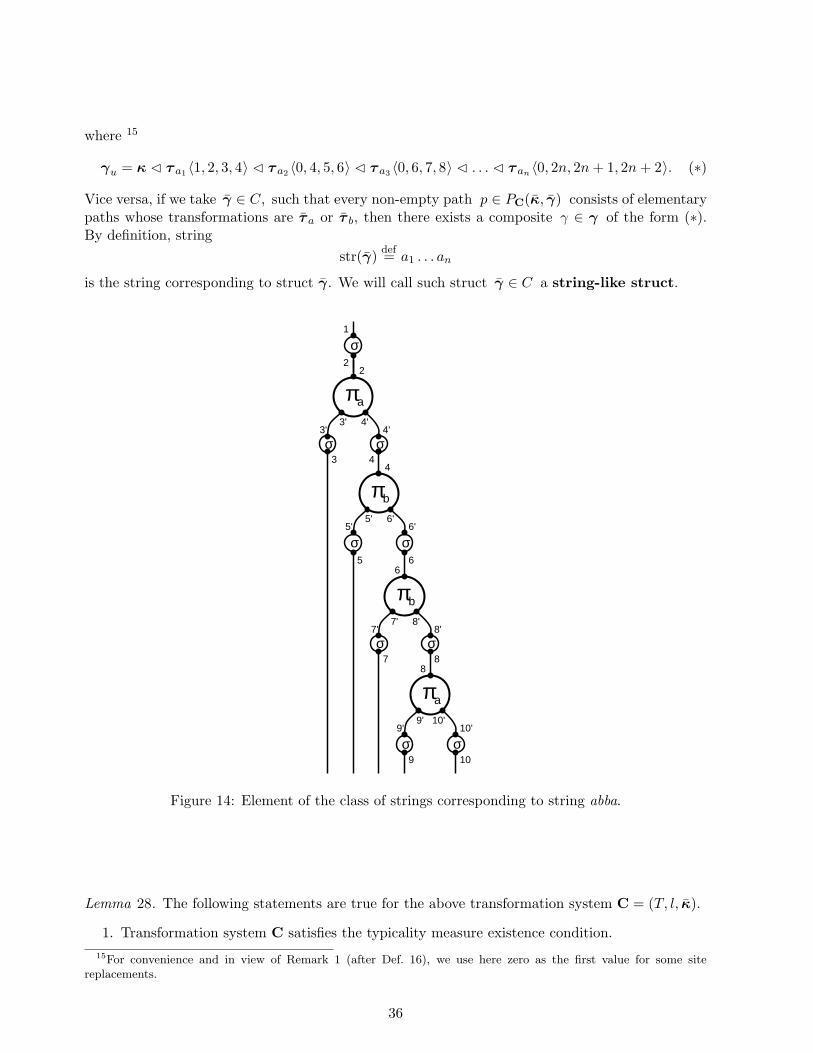
γu = κ C τ a1 〈1, 2, 3, 4〉 C τ a2 〈0, 4, 5, 6〉 C τ a3 〈0, 6, 7, 8〉 C . . . C τ an 〈0, 2n, 2n + 1, 2n + 2〉. (∗)

Vice versa, if we take γ ∈ C, such that every non-empty path p ∈ PC(κ, γ) consists of elementarypaths whose transformations are τ a or τ b, then there exists a composite γ ∈ γ of the form (∗).By definition, string

str(γ) def= a1 . . . an

is the string corresponding to struct γ. We will call such struct γ ∈ C a string-like struct.

πa

2

1

4'3'

3

4'

σ2

3'

πb

4

6'5'

5

6'

6

4

5'

πb

6

8'7'

7

8'

8

7'

πa

8

10'9'

9

10'

10

9'

σσ

σ

σσ

σ σ

σ

Figure 14: Element of the class of strings corresponding to string abba.

Lemma 28. The following statements are true for the above transformation system C = (T, l, κ).

1. Transformation system C satisfies the typicality measure existence condition.15For convenience and in view of Remark 1 (after Def. 16), we use here zero as the first value for some site

replacements.

36

λ

aτx

τa τb

bτx

τxx

τa

τa

aa

τx

τxx

τa

τa

τb

τb τb

τb

ab ba bb

Figure 15: Paths and elements of the class of strings. String-like structs are labeled by the corre-sponding strings, and elementary paths are labeled by their transformations.

2. For γ ∈ C,

νC(γ) =

2

3n+1(n+1) ln 3, if γ is a string-like struct corresponding to a string of length n

0 , otherwise.

Proof. Take γ ∈ C.If γ is not a string-like struct, then either there exists an elementary path whose transformation

is τ xx from EPC(γ), which the generating process choses with probability 1 (since l(τ xx) = 0), orEPC(γ) = ∅. In either case, since l(τ xx) = 0, the expected time spent by the generating processin γ is 0.

If γ is a string-like struct corresponding to a string of length n, then the probability that thegenerating process passes a particular path p ∈ PC(κ, γ) is equal to

13· 16· . . . · 1

3n=

13nn!

.

There are n! paths in PC(κ, γ) (see Fig. 15). Hence, the probability that process G reaches γ is1/3n. Since for all elementary paths s ∈ EPC(γ), l(s) = 1, and there are 3(n + 1) of them, theexpected time spent by the process in γ is equal to 1/(3n · 3(n + 1)), i.e. EG(γ) = 1/(3n+1(n + 1)).

Since the string-like structs and strings are in one-to-one correspondence,

EG =∑

u∈a,b∗EG(γu) =

∞∑

n=0

2n

3n+1(n + 1)=

ln 32

.

Thus, C satisfies the typicality measure existence condition, and

νC(γ) =EG(γ)

EG=

23n+1(n + 1) ln 3

.

¥We will denote the constructed class of strings C in ESIS as Cstr.

37

3.8 Natural numbers inductive structure and the class of natural numbers

For this inductive structure, the set of abstract sites is A = a1, a2 and the set of concrete sites isS = 0, 1, 2, . . .. The set of primtypes for the natural numbers inductive structure is ΠN = π1, πx,where

init(π1) = init(πx) = a1term(π1) = a2term(πx) = ∅

The set of semantic identities is IN = Comm(ΠN), i.e. the set of commutativity identities (seeDef. 13).

The transformation set for the class of natural numbers is T = τ 1, τ x, where

τ 1 = ([π1〈1, 2〉], [π1〈1, 2〉 C π1〈2, 3〉])τ x = ([π1〈1, 2〉], [π1〈1, 2〉 C πx〈2〉]).

The transformation weights are defined as follows

l(τ 1) = l(τ x) = 1,

and the progenitor is κ = [π1〈1, 2〉]. We will call CN = (T, l, κ) the transformation system fornatural numbers.

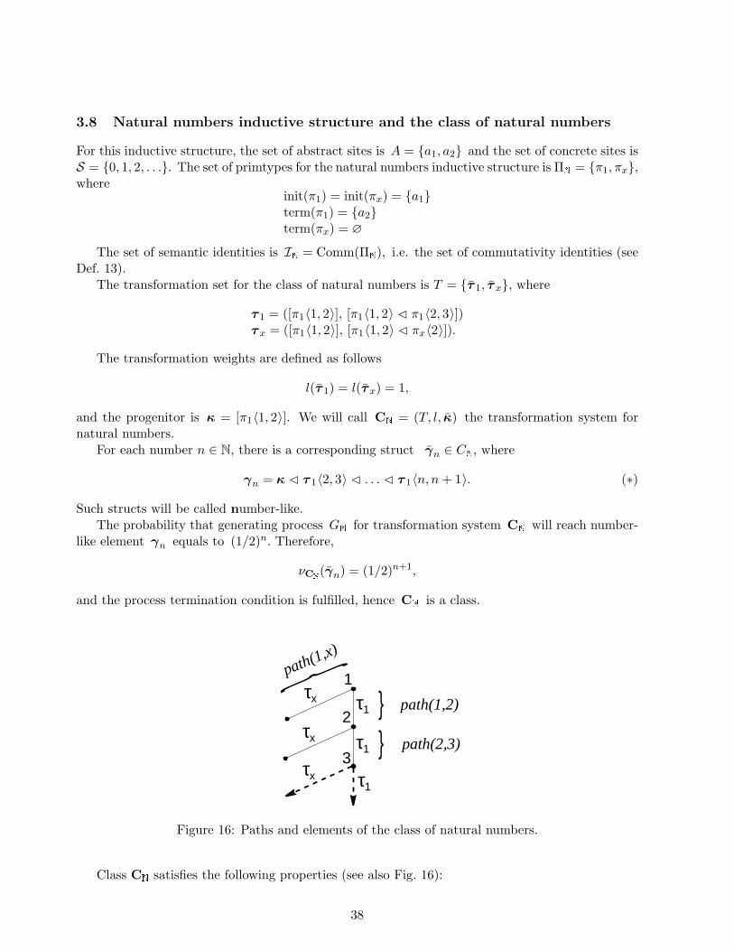
For each number n ∈ N, there is a corresponding struct γn ∈ CN, where

γn = κ C τ 1〈2, 3〉 C . . . C τ 1〈n, n + 1〉. (∗)

Such structs will be called number-like.The probability that generating process GN for transformation system CN will reach number-

like element γn equals to (1/2)n. Therefore,

νCN(γn) = (1/2)n+1,

and the process termination condition is fulfilled, hence CN is a class.

1τ1

τ1

2

3

τx

τx

τx τ1

path(1,2)

path(2,3)

path(1,x)

Figure 16: Paths and elements of the class of natural numbers.

Class CN satisfies the following properties (see also Fig. 16):

38

1. For every pair of natural numbers (m, n), m < n, there exists unique path in PCN betweenγm and γn, which we denote by path(m,n).

2. For every natural number n, there exists unique elementary path in EPCN beginning at γn

whose transformation is τ x. We denote this path by path(n, x).

3. For all natural numbers m,n, k,

path(m,n) → path(k + m, k + n)path(n, x) → path(n + k, x)path(n, x) path(m,n) → path(n + k, x) path(m + k, n + k).

3.9 Category of classes and class morphisms

In this and the next sections, we formalize the intuitive understanding of the relationship betweenthe classes of (possibly different) inductive structures by introducing the concept of morphism [25].In mathematics, a morphism between two analogous/homogeneous “mathematical structures” isa mapping which “carries” each operation in the domain into the corresponding operation in thecodomain. Since, in this paper, our immediate goal is inductive learning of classes, the “mathemat-ical structures” of interest are classes, and, therefore, the “structural elements” are paths. Earlier,we have defined three operations on paths: composition, embedding, and path duration.

We verify that the set of all classes (in all inductive structures) and morphisms between themform a category. The concepts of monomorphism (in the category of sets these correspond toinjective mappings) and epimorphism (those corresponding to surjective mappings), as well as thoseof a subclass and a quotient-class follow from the definition of morphism in a standard manner.However, in view of its immediate utility, we will give, in the next (very short) section, explicitdefinition of a monomorphism.

Definition 37. Let C1 = (T1, l1, κ1), C2 = (T2, l2, κ2) be classes from inductive structures(Π1, I1), (Π2, I2) respectively. A morphism f from C1 to C2, denoted

f : C1 → C2,

is specified by a mapping f : PT1 → PT2 satisfying for all p1, p2, p ∈ PT1 the following conditions:

1. f(p1 p2) = f(p1) f(p2).

2. If p1 → p2, then f(p1) → f(p2).

3. l2(f(p)) = l1(p).

Two morphisms, f1 : C1 → C2 and f2 : C1 → C2, are equal, if the corresponding mappings f1

and f2 coincide on every path that the generating process G1 for C1 can pass 16. I

Example 7. We now define a morphism f : CN → Cstr. Due to property 3 (applied to CN), it issufficient to define the mapping f on paths path(1, 2), path(2, 3), path(1, x) and path(2, x). Indeed,let the values of mapping f on these paths be fixed. We, first, prove that f(path(3, 4)) is uniquelydefined.

16See Remark 3 (section 3.6).

39

• Since path(1, 2) → path(2, 3) → path(3, 4),

f(path(1, 2)) → f(path(3, 4)) → f(path(3, 4)).

• Since path(1, 3) → path(2, 4), we have

f(path(2, 3)) f(path(1, 2)) = f(path(2, 3) path(1, 2)) = f(path(1, 3)) →f(path(2, 4)) = f(path(3, 4) path(2, 3)) = f(path(3, 4)) f(path(2, 3)).

The statement follows directly from the above two facts.Similarly, we see that f(path(n, n + 1)) is uniquely defined for all n ∈ N.Next, for all n ∈ N,

path(2, x) path(1, 2) → path(n + 1, x) path(n, n + 1),

therefore f(path(n + 1, x)) is uniquely defined.To complete the proof, we note that since the values of f are uniquely defined on all elementary

paths, f itself is uniquely defined.Obviously, the values f(path(1, 2)), f(path(2, 3)), f(path(1, x)) and f(path(2, x)) can be spec-

ified in infinitely many ways. Let us look at one of them:

f1(path(1, 2)) = [ (κstr, τ a〈1, 2, 3, 4〉, κstr C τ a〈1, 2, 3, 4〉) ]f1(path(2, 3)) = [ (κstr C τ a〈1, 2, 3, 4〉, τ a〈0, 4, 5, 6〉, κstr C τ a〈1, 2, 3, 4〉 C τ a〈0, 4, 5, 6〉) ]f1(path(1, x)) = [ (κstr, τ x〈1, 2, 3〉, κstr C τ x〈1, 2, 3〉) ]f1(path(2, x)) = [ (κstr C τ a〈1, 2, 3, 4〉, τ x〈0, 4, 5〉, κstr C τ a〈1, 2, 3, 4〉 C τ x〈0, 4, 5〉) ].

In this case, the progenitor of CN is mapped onto the progenitor of Cstr corresponding to thenull string, and, in general, struct γn is mapped onto γan−1 (here structs are considered as pathsof length 0). Furthermore, every elementary path in CN is mapped into the elementary path inCstr corresponding to the insertion of letter a at the end of the string. Finally, the terminationelementary paths path(n, x) are mapped onto the termination elementary paths for Cstr .

For each thus specified mapping f , since the path durantion is, obviously, preserved, f definesa morphism. ♦

Remark 5. We conjecture that, in general, any morphism can be uniquely and finitely specified byits values on certain “basic” paths.

Next, we check the categorical properties of morphisms, i.e. the existence of compositions ofmorphisms and of the identity morphism, and the associativity of the composition.

Definition 38. For two morphisms f : C1 → C2 and g : C2 → C3, the composition of f and g,denoted g f , is a morphism h : C1 → C3, where h = g f. I

Lemma 29. The above definition of composition is correct, i.e. mapping h satisfies the conditionsin Def. 37.

40

Lemma 30. The composition of morphisms is associative, i.e. for any classes C1, C2, C3, C4 andmorphisms f : C1 → C2, g : C2 → C3, h : C3 → C4,

h (g f) = (h g) f .

Lemma 31. For a class C = (T, l, κ), the identity path mapping id : PT → PT defines the identityclass morphism idC : C → C, i.e. for any morphisms g : C1 → C and h : C → C2,

idC g = g and h idC = h.

Thus, the set of all classes forms a category which is natural to call the category of classes.

Definition 39. Two classes C1, C2 will be called isomorphic, if there exist morphisms f : C1 →C2, g : C2 → C1 such that f g = idC1 and g f = idC2 . I

3.10 Subclasses and struct representations

In this (short) section, we introduce important concepts of subclass and struct representation.

Definition 40. Morphism f : C1 → C2 will be called a monomorphism, if for any pair of distinctpaths p1, p2 that the generating process of class C1 can pass,

f(p1) 6= f(p2).

A monomorphism will be denoted by f : C1 → C2. For class C, a subclass is defined as a pair(f ,C′), where f : C′ → C. I

Lemma 32. A morphism f : C1 → C2 is a monomorphism, if and only if, for any class C and forany morphisms g,h : C → C1, g 6= h implies f g 6= f h.

Important remark. Suppose that an agent has knowledge of several classes, some of which arerelated to each other via monomorphisms. When the agent encounters a “physical” object, he at-tempts to construct a “representation” of the object by discovering its formative history based on theagent’s knowledge of some classes, i.e. the classes activated by the object. The agent accomplishesthis by initiating the generating process for each of these classes. Each such process is conditionedby the above relationship (via monomorphisms) between the classes and simultaneously “guided”by the agent’s structural measurement devices. The function of the structural measurement deviceis to match the structs from some of the active classes against the original “physical” object. Foreach of the active classes, the current state, or struct, of the corresponding generating process canbe called the current representation of the “physical” object with respect to that class.

Definition 41. For a struct γ ∈ C, the representation of γ with respect to a subclass(f ,C′) is defined as a pair (f−1(γ), C′). I

Note that the “explicit” representation of struct γ with respect to class C is also not uniqueand is associated with a particular path from the class progenitor to γ.

41

4 The learning problem

In this, our “destination”, section we briefly outline a tentative formulation of the learning problem.

We assume that (Π, I) is a fixed inductive structure and all classes that we consider are classesin this inductive structure. Let C be a fixed class in (Π, I) which will be called the superclassand from which the learning subclasses will be selected.

First, we hypothesize that there exists unique class P(C) called the power class of C, whichhas the following properties:

• there exists a bijection between P(C) and the set all subclasses of C; for each subclass (f ,K)of C, the corresponding element of P(C) will be denoted as ξ(f ,K) and should be thoughtof as the “representation” of that subclass

• its progenitor κP(C) corresponds to class C itself:

ξ(idC,C) = κP(C)

• transformations of class P(C) should be thought of as the “building blocks” with which therepresentation of any subclass of C (including its monomorphism) can be constructed.

Thus, one can think of the generating process GP(C) for this superclass as the one constructingthe representations of the subclasses of C. Note that since P(C) is uniquely defined by C, GP(C)

is also uniquely defined.

Definition 42. For a subclass (f ,K) of C, a finite subset R ⊂ f(K) will be called a trainingset generated by (f ,K). Let us define the typicality of a training set R = α1, . . . , αn as

ν(f ,K)(R) def=n∏

i=1

νK(f−1(αi)). (14)

I

Next, let us suppose that we know the transformation system for superclass C, which we will nowconsider as an “external” class, and suppose that we are observing an external generating processfor the power class P(C), and, moreover, suppose that, during our observation, this process remainsin state ξ(f ,K). It is natural to assume that we do not know the struct ξ(f ,K) or, in other words,we do not know the representation of subclass (f ,K). Then, suppose we observed a training setR′ = γ1, . . . , γn generated by (f ,K) . We consider elements of the training set R′ as independentdiscrete random variables whose values belong to set f(K),17 and

Prob(γi = γ) = νK(f−1(γ)), i ∈ [1, n], γ ∈ f(K). (15)

For a finite subset R ⊂ C, let us denote by ER the random event “R′ = R”, and by E(f ,K) therandom event “R′ is generated by subclass (f ,K)”. Note that event E(f ,K) can also be describedas “GP(C) is in state ξ(f ,K)”. By Def. 35, the probability of event E(f ,K) is

Prob(E(f ,K)) = νP(C)(ξ(f ,K)). (16)

17See, for example, [26].

42

According to (14, 15), the probability of the conditional event “R′ = R under condition thatR′ is generated by subclass (f ,K)” is given by formula

Prob(ER | E(f ,K)) = ν(f ,K)(R).18 (17)

Now, the learning problem can be formulated as follows: given a finite subset R0 ⊂ C, findsubclass (f0,K0) for which the conditional probability

Prob(E(f0,K0) | ER0) (∗)

is maximal. In other words, the learning problem is to find subclass (f0,K0) whose generatingprocess is most likely to generate the observed set R0.

For conditional probability (∗), we have:

Prob(E(f0,K0) | ER0) =Prob(ER0 | E(f0,K0)) · Prob(E(f0,K0))

Prob(ER0).

Since the training set R0 is fixed, the denominator is also fixed, and (∗) is maximal whenever thenumerator is maximal. From (17, 16), we obtain

Prob(ER0 | E(f0,K0)) · Prob(E(f0,K0)) = ν(f0,K0)(R0) · νP(C)(ξ(f0,K0)),

so the learning problem is equivalent to the following one: given R0, find subclass (f0,K0) whichmaximizes

ν(f0,K0)(R0) · νP(C)(ξ(f0,K0)). (∗∗)

We will not give a precise definition of the above power class but simply note that it has to bedefined as an instance of the general categorical concept of power object specified for our categoryof classes. Therefore, instead of evaluating the second factor in (∗∗) directly, for practical purposes,we replace this factor by a “similar” one as explained next.

Let τ be a transformation from the transformation set that defines class K. Choose anyitransformation τ = (α, β) ∈ τ , and denote by p the elementary path which contains elementaryipath (α, τ ,β). It is easy to check that p is correctly defined.

For a subclass (f ,K) of C, where K = (τ 1, . . . , τm, l, κ), let us call

νC(f ,K) def= νC(f(κ)) ·m∏

i=1

µC(f(p i))

the typicality of subclass (f ,K), where µC is the path probability measure (see Def. 36). Then,we can replace the second factor in (∗∗), which is the typicality of the representation ξ(f0,K0) ofsubclass (f0,K0) in power class P(C), by the typicality of subclass (f0,K0).

Thus, the learning problem can now be formulated as follows: given R0, find subclass (f0,K0)which maximizes

ν(f0,K0)(R0) ·

[νC(f(κ)) ·

m∏

i=1

µC(f(p i))

].19

18See Appendix for a proof of this equality.19For the classical case see, for example, [27].

43

Preliminary analysis suggests that this optimization problem has a non-trivial solution whichcorresponds to a subclass (f0,K0) lying “between” two extreme non-optimal solutions: one corre-sponding to the superclass C, and the other one, to the smallest subclass containing R0.

Finally, it is important to note that, as a result of the learning process, a new object represen-tation (see Def. 41), i.e. the pair (f−1(γ), K), of an object originally represented as (γ,C) may“take over”: the typicality of f−1(γ) in K might be higher than the typicality of γ in C.

5 Future work

First of all, we want to come back to the Introduction and discuss very briefly the questions ofexplanatory value of the ETS model as well as of its experimental “verification”. One might say thatthe description of the class by means of its transformation system encapsulates the explanatorynature of the outlined model: it suggests what the representation (or “nature”) of the class is,or how to “think” about a class of objects, including the interpretation of transformations asclass “features”. At the same time, the experimental verification of the model might also beapproached from the point of view of validity of this explanatory hypothesis about the nature ofclass representation. It turns out that in cognitive psychology there has already accumulated someexperimental evidence supporting the model (starting from the work of M.I.Posner and co-workersand J.J.Franks and J.D.Bransford [28]). We are currently working on the initial verification of thishypothesis for some classes of organic molecules. It is understood, that to properly conduct theexperimental work the form of data representation must confirm to the proposed structural formof representation, which, in turn, requires rethinking of the conventional forms of representation.

As far as the theory is concerned, below we list some of the important topics (most are verysubstantial) for the future research.

• Investigate the axiomatics for the inductive structure.

• Develop a theory of inductive structures (potentially of great importance for mathematicsand sciences).

• Introduce a natural hierarchy of (non-isomorphic) inductive structures and show that theanalogues of the numeric representations are the simplest ones.

• Are there any other natural ways to introduce the transformations?

• Introduce a natural hierarchy of transformation systems.

• Is there a different/interesting approach, not relying on stochastic processes, to the generationof class elements?

• Should one allow the classes with several progenitors and how to define such classes?

• Introduce the concept of morphism for inductive structures and investigate the alternativedefinitions of the class morphism.

• Propose a formal definition of the power class.

• Propose an alternative formulation of the learning problem.

44

• Investigate various stages of the learning process (together with the relevant concepts).

• Develop a powerful machinery (and optimization theory) for efficient construction of the classtransformation system during the learning process.

Acknowledgment

We would like to thank John Abela for encouraging us to undertake this work sooner rather thanlater.

Appendix

Here we define accurately the random variables considered in Section 4, and prove formula (17).Let (Ω1,B1, Prob1) be a probability space, and let

sc : Ω1 → P(C)

be a random variable with the values in the power class P(C) which has the following meaning:for ω1 ∈ Ω1,

sc(ω1) = ξ(f ,K)

denotes a random subclass (f ,K) of C generated by the generating process of P(C).After the generating process of P(C) generates the subclass (f ,K), the generating process for

subclass (f ,K) generates a training set.Let (Ω2,B2, Prob2) be a probability space, and assume that for every subclass (f ,K) of C there

exist independent random variables

tKi : Ω2 → K, i ∈ [1, n]

corresponding to the elements of a training set for class K.Consider the product of the introduced probability spaces

(Ω,B, Prob) = (Ω1 × Ω2, B1 × B2, Prob1×Prob2)

and random variablesti : Ω → C, 20 i ∈ [1, n]

defined asti(ω1, ω2)

def= f(tKi (ω2)

), where (f ,K) is such that ξ(f ,K) = sc(ω1).

Thus, ti(ω1, ω2) | i ∈ [1, n] is the image in C of a random training set for a random subclass(f ,K). Suppose we observed a particular training set R = γ1, . . . , γn ⊂ C. The conditionalprobability in the left hand side of (17) can now be rewritten as

Prob(ER | E(f ,K)) = Prob[t1(ω1, ω2) = γ1 , . . . , tn(ω1, ω2) = γn

∣∣ sc(ω1) = ξ(f ,K)

]=

=Prob

[t1(ω1, ω2) = γ1 , . . . , tn(ω1, ω2) = γn , sc(ω1) = ξ(f ,K)

]

Prob(sc(ω1) = ξ(f ,K)

) =Prob(X)Prob(Y )

,

20It is not hard to see that ti are indeed random variables, i.e. inverse image of any element in C is a measurablesubset of Ω2.

45

where

X =

(ω1, ω2) ∈ Ω∣∣ t1(ω1, ω2) = γ1 , . . . , tn(ω1, ω2) = γn, sc(ω1) = ξ(f ,K)

Y =

(ω1, ω2) ∈ Ω∣∣ sc(ω1) = ξ(f ,K)

.

IfX1 =

ω1 ∈ Ω1

∣∣ sc(ω1) = ξ(f ,K)

X2 =

ω2 ∈ Ω2

∣∣ f(tK1 (ω2)

)= γ1 , . . . , f

(tKn (ω2)

)= γn

,

then X = X1 ×X2, Y = X1 × Ω2, and, according to [26, Remark 35.13],

Prob(X) = Prob1(X1) · Prob2(X2)Prob(Y ) = Prob1(X1).

Since tKi , i ∈ [1, n], are independent random variables,

Prob2(X2) = Prob2

[f(tK1 (ω2)

)= γ1 , . . . , f

(tKn (ω2)

)= γn

]=

Prob2

[f(tK1 (ω2)

)= γ1

] · . . . · Prob2

[f(tKn (ω2)

)= γn

]= ν(f ,K)(R).

Hence,

Prob(ER | E(f ,K)) =Prob(X)Prob(Y )

=Prob1(X1) Prob2(X2)

Prob1(X1)= ν(f ,K)(R),

and (17) is proved.

References

[1] G. Sarton, Ancient Science Through the Golden Age of Greece, Dover, New York, 1993.

[2] G. Ifrah, The Universal History of Numbers, J. Wiley, New York, 2000.

[3] E. Schrodinger, Nature and the Greeks and Science and Humanism, pp.143-145, 158, CUP,Cambridge, UK, 1996.

[4] L. Goldfarb, On the foundations of intelligent processes I: An evolving model for pattern learn-ing, Pattern Recognition 23 (6) (1990), 595-616.

[5] L. Goldfarb, What is distance and why do we need the metric model for pattern learning,Pattern Recognition 25 (4) (1992), 431-438.

[6] L. Goldfarb, S. Nigam, The unified learning paradigm: A foundation for AI, in: V. Honavar,L. Uhr (Ed.), Artificial Intelligence and Neural Networks: Steps toward Principled Integration,1994, pp. 533-559.

[7] L. Goldfarb, J. Abela, V. C. Bhavsar, V. N. Kamat, Can a vector space based learning modeldiscover inductive class generalization in a symbolic environment? Pattern Recognition Letters16 (7) (1995) 719-726.

[8] L. Goldfarb, Inductive class representation and its central role in pattern recognition, Proc.Conf. Intelligent Systems: A Semiotic Perspective, Vol. 1, NIST, Gaithersburg, Maryland,USA, 1996, pp. 53-58.

46

[9] L. Goldfarb, What is inductive learning?: Construction of inductive class representation, Proc.Workshop ”What Is Inductive Learning” in Conjunction with 11th Biennial Canadian AI Conf.,1996, pp. 9-21.

[10] L. Goldfarb, S. Deshpande, What is a symbolic measurement process?, Proc. IEEE Conf.Systems, Man, and Cybernetics, Vol. 5, Orlando, Florida, USA, 1997, pp. 4139-4145.

[11] L. Goldfarb, J. Hook, Why classical models for pattern recognition are not pattern recognitionmodels, Proc. Intern. Conf. On Advances in Pattern Recognition, Plymouth, UK, 1998, pp.405-414.

[12] E. G. H. Landau, Foundations of Analysis, Chelsea, New York, 1951.

[13] C. Lee, Notes for Math 502, 1998 [http://www.ms.uky.edu/ lee/ma502/notes2/node7.html].

[14] M.A. Aiserman, Remarks on two problems connected with pattern recognition, in: S. Watan-abe (Ed.), Methodologies of Pattern Recognition, , p.1, Academic Press, 1969.

[15] J. Losee, A Historical Introduction to the Philosophy of Science, 3rd ed., OUP, Oxford, 1993.

[16] A. Bird, Philosophy of Science, McGill-Queen’s University Press, Montreal, 1998.

[17] J. H. Holland, K. J. Holyoak, R. E. Nisbett, P. R. Thagard, Induction, MIT Press, Cambridge,Mass., 1986.

[18] M. Piattelli -Palmarini (Ed.), Language and Learning: The Debate between Jean Piaget andNoam Chomsky, pp. 100-103, 255-272, HUP, Cambridge, USA, 1980.

[19] N. Chomsky, Knowledge of Language: Its Nature, Origin, and Use, p. 12, Praeger, New York,1986.

[20] D. Wolpert, Preface, in: D. Wolpert (Ed.), The Mathematics of Generalization, p.8, Addison-Wesley, Reading, MA, USA, 1995.

[21] A.R. Lacey, A Dictionary of Philosophy, 3rd ed., p. 308, Routledge, London, UK, 1996.

[22] R. Dunbar, The Trouble with Science, p. 17, Faber and Faber, London, UK, 1996.

[23] N. Chomsky, Syntactic Structures, Mouton, London, The Haugue, The Netherlands, 1965.

[24] A.G. Kurosh, Lectures on General Algebra, Section 1.5, Chelsea, New York, 1963.

[25] S. MacLane, G. Birkhoff, Algebra, 3rd ed., Chelsea, New York, 1993.

[26] K.R. Parthasarathy, Introduction to Probability and Measure, Sections 3, 22, Macmillan IndiaPress, Madras, 1977.

[27] T.M. Mitchell, Machine Learning, Sections 6.3, 6.9, McGraw-Hill, Boston, 1997.

[28] J.J. Franks, J.D. Bransford, Abstraction of visual patterns, J. of Experimental Psychology 90(1) (1971) 65-74.

47