What is a Question?

Kevin H. Knuth

NASA Ames Research Center, Computational Sciences Department, Code [C

Moffett Field CA 94035 USA

Abstract. A given question can be defined in terms of the set of statements or assertions that

answer it. Application of the logic of inference to this set of assertions allows one to derive the

logic of inquiry amor_g questions. There are interesting symmetries between the logics of

inference and inquiry; where probability describes the degree to which a premise implies an

assertion, there exists an analogous quantity that describes the bearing or relevance that a

question has on an ou standing issue. These have been extended to suggest that the logic of

inquiry results infunct onal relationships analogous to;- although more general than; those found

in information theory.

Employing lattice theory, I examine in greater detail the structure of the space of assertions

and questions demonstrating that the symmetries between the logical relations in each of the

spaces derive directly from the lattice structure. Furthermore, I show that while symmetries

between the spaces exist., the two lattices are not isomorphic. The lattice of assertions is

described by a Boolean lattice 2", whereas the lattice of real questions is shown to be a

sublattice of the free distributive lattice FD(N) = 2 z'v . Thus there does not exist a one-to-one

mapping of assertions t_ questions, there is no reflection symmetry between the two spaces, and

questions in general do not possess unique complements. Last, with these lattice structures in

mind, I discuss the reIat onship between probability, relevance and entropy.

"Man has made some machines that can answer questions provided theft acts

are profusely stored in them, but we will never be able to make a machine that

will ask questions. The ability to ask the right question is more than half the

battle of finding the answer."- Thomas J. Watson (1874-1956)

INTRODUCTION

It was demonstra}ed b3 RiChard-;I'. COX (I 9_46, -1-561) that-probability theory-represents

a generalization of Boolean implication to a degree of implication represented by areal number. This insight has placed probability theory on solid ground as a calculus

for conducting inductive inference. While at this stage this work is undoubtedly his

greatest contribution, his ultimate paper, which takes steps to derive the logic of

questions in terms of the set of assertions that answer them, may prove yet to be themost revolutionary. While much work has been done extending and applying Cox's

results (Fry 1995, 1998, 2000; Fry & Sova 1998; Bierbaum & Fry 2002; Knuth 2001,

2002), the structure of _:hespace of questions remains poorly understood. In this paper

https://ntrs.nasa.gov/search.jsp?R=20020070851 2018-07-07T09:19:53+00:00Z

I employ lattice theory to describethe structureof the spaceof assertionsanddemonstratehowlogicalimplicationontheBooleanlatticeprovidestheframeworkonwhichthecalculusof inductiveinferenceisconstructed.I thenintroducequestionsbyfollowingCox (l 979) and defining a question in terms of the set of assertions that cananswer it. The lattice structure of questions is then explored and the calculus for

manipulating the relevance of a question to an unresolved issue is examined.

The first section is devoted to the formalism behind the concepts of partially ordered

sets and lattices. The second section deals with the logic of assertions and introducesBoolean lattices. In the third section, I introduce the definition of a question and

introduce the concept of an ideal question. From the set of ideal questions I construct

the entire question lattice identifying it as a free distributive lattice. Assuredly realquestions are then shown to comprise a sublattice of the entire lattice of questions. In

the last section I discuss the relationship between probability, relevance, and entropyin the context of the lattice structure of these spaces.

FORMALISM

Partially Ordered Sets

In this section I begin with the concept of a partially ordered set, called aposet, which

is defined as a set with a binary ordering relation denoted by a _ b, which satisfies for

all a, b, c (Birkhoff 1967):

P1. For all a, a < a. (Reflexive)

P2. If a _ b and b _ a, then a = b (Antisymmetry)

P3. If a < b and b < c, then a < c (Transitivity)

Alternatively one can write a < b as b :- a and read "b contains a" or "b includes a".

If a < b and a b one can write a < b and read "a is less than b" or "a is properly

contained in b". Furthermore, if a < b, but a < x < b is not true for any x in the poset

P, then we say that "b covers a", written a -<b. In this case b can be considered an

immediate superior to a in a hierarchy. The set of natural numbers {1, 2, 3, 4, 5}

along with the binary relation "less than or equal to" < is an example of a poset. In

-this pose ,tv-the-number--3 eovers-the number-2-as-2 <-3Tbut--there-is-no-number-x-in-the

set where 2 < x < 3. This covering relation is useful in constructing diagrams to

visualize the structure imposed on these sets by the binary relation.

To demonstrate the construction of these diagrams, consider the poset defined bythe powerset of {a,b,c} with the binary relation _.C read "is a subset of",

P=({{_},{a},{b},{c},{a,b},{b,c},{a,c},{a,b,c}} C_) where the powerset

_(X) of a set X is the set of all possible subsets of X. As an example, it is true

that{a} C {a,b,c}, read "{a} is included in {a,b,c}". Furthermore, it is true that

{a} C {a,b,c}, read "{a} is properly contained in {a,b,c}'" as {a} C {a,b,c}, but

{a} {a,b,c}. Hoaever, {a,b,c} doesnotcover {a} as {a}C{a,b}C{a,b,c}.Wecanconstructadiagram(Figure1)bychoosingtwoelementsx andy from the set,and writing y above x when x C y. In addition, we connect two elements x and y with

a line when y covers ,_, x < y.

Posets also posse._.s a duality in the sense that the converse of any partial orderingis itselfa partial ordering (Birkhoff 1967). This is known as the duality principle and

can be understood b_ changing the ordering relation "is included in" to "includes"

which equates graphically to flipping the poset diagram upside-down.

With these examples of posets in mind, I must briefly describe a few moreconcepts. If one considers a subset X of a poset P, we can talk about an element a _P

that contains every element x_X; such an element is called an upper bound of the

subsetX. The least ut,per bound, or l.u.b., is an element in P, which is an upper boundof Xand is contained in every other upper bound of X. Thus the I.u.b. can be thought

of as the immediate successor to the subset X as one moves up the hierarchy. Dually

we can define the greatest lower bound, or g.l.b. The least element of a subset Xis an

element a_X siich ttat a _x for all x_X . The gied-te:_t elO_-ent _s defiri6d dually.

{a,b,c}

/1\a,b} {a,c} {b,c}

IX Xi{a} {b} {c}

\1/{0}

FIGURE 1. Theposet P = ({_3},{a} {b},{c},{a,b},{b, cI,{a,c},{a,b,c}}, _C) results inthe

diagram shown here. The binary relation _C dictates the height of an element in the diagram. Theconcept of covering alIows us to draw lines between a pair of elements signifying that the higherelement in the pair is an mmediate successor in the hierarchy. Note that {a} is covered by twoelements. These diagrams nicely illustrate the structural properties of the poser. The element {a, b, c }

is the greatest element ofP md{ O } is the least element of P.

Lattices

-T-he-next-important concept-is-the lattice. A-lattice is a poset/?-where every-pair of

elements x and y has a least upper bound called the join, denoted as x v y, and a

greatest lower bound called the meet, denoted by x ^ y. The meet and join obey the

following relations (Bil khoff 1967):

L1. XAX=X, xv r=x (Idempotent)

L2. XAy=yAX, xvy=yvx (Commutative)

L3. x 6 (y ^ z) = (x ^ y) A Z, X V (y V Z) = (X V y) V Z (Associative)

L4. x ^ (x v y) = x ', (x A y) = X (Absorption)

In addition,for elementsx and y that satisfy x < y their meet and join satisfy the

consistency relations

C1. x^ y=x

C2. xvy=y

(x is the greatest lower bound ofx and y)

(v is the least upper bound ofx andy).

The relations L1-4 above come in pairs related by the duality principle; as they hold

equally for a lattice L and its dual lattice (denoted L°), which is obtained by reversingthe ordering relation thus exchanging upper bounds for lower bounds and hence

exchanging joins and meets. Note that the meet and join are generally defined for all

lattices satisfying the definition of a lattice; even though the notation is the same they

should not be confused with the logical conjunction and disjunction, which refer to aspecific ordering relation. I will get to how they are related and we will see that lattice

theory provides a general framework that clears up some mysteries surrounding thespace of assertions and the space of questions.

THE LOGIC OF ASSERTIONS

Boolean Lattices

I introduce the concept of a Boolean lattice, which possesses structure in addition to

L1-4. A Boolean lattice is a distributive lattice satisfying the following identities forall x, y, z:

x ^ (y v z) = (x ^ y) v (x ^ z)B 1. (Distributive)

x v (y ^ z) = (x v y) ^ (x v z)

Again the two identities are related by the duality principle. Last the Boolean lattice isa complemented lattice, such that each element x has one and only one complement

x that satisfies (Birkhoff 1967):

B2.

-B3.

B4.

XA-x=O xv-x=I

-(x^ y)---xv-y -(xvy)=-x^-y

where O and I are the least and greatest elements, respectively, of the lattice. Thus a

Boolean lattice is a complemented distributive lattice.

We now consider a specific application where the elements a and b are logical

assertions and the ordering relation is x<y = x_y, read "x implies y". The logical

operations of conjunction and disjunction can be used to generate a set of four logicalstatements, which with the binary relation "implies" forms a Boolean lattice displayed

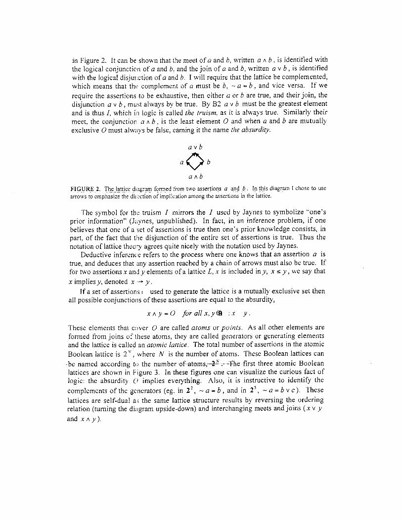
in Figure2. It canbeshownthatthemeetof a and b, written a A b, is identified with

the logical conjunctic.n of a and b, and the join of a and b, written a v b, is identified

with the logical disjm:ction of a and b. I will require that the lattice be complemented,

which means that the complement of a must be b, _ a -- b, and vice versa. If we

require the assertions to be exhaustive, then either a or b are true, and their join, thedisjunction a v b, mu:_t always by be true. By B2 a v b must be the greatest element

and is thus I, which i_l logic is called the truism, as it is always true. Similarly their

meet, the conjunction a A b, is the least element O and when a and b are mutually

exclusive O must alw_tys be false, earning it the name the absurdity.

avb

aAb

FI_G.URE2. The lattice diagram form.ed from two assertions a _and b. In tt?isdiagram I chose to usearrows to emphasize the diz_'ctionof implication among the assertions in the lattice.

The symbol for the truism I mirrors the I used by Jaynes to symbolize "one's

prior information" (Jaynes, unpublished). In fact, in an inference problem, if onebelieves that one of a set of assertions is true then one's prior knowledge consists, in

part, of the fact that the disjunction of the entire set of assertions is true. Thus the

notation of lattice theo-y agrees quite nicely with the notation used by Jaynes.

Deductive inference refers to the process where one knows that an assertion a is

true, and deduces that any assertion reached by a chain of arrows must also be true. If

for two assertions x andy elements of a lattice L, x is included iny, x _ y, we say that

x impliesy, denoted x ---, y.

Ifa set of assertions I used to generate the lattice is a mutually exclusive set then

all possible conjunctions of these assertions are equal to the absurdity,

x A y = O for all x, y_tt : x y .

These elements that c_ver O are called atoms or points. As all other elements are

formed from joins of these atoms, they are called generators or generating elementsand the lattice is called an atomic lattice. The total number of assertions in the atomic

Boolean lattice is 2 v i where N is the number of atoms. These Boolean lattices can

-be-named aceord-ing t_--the--number-of-atoms,-2 --N..--The first-three atomic-Boolean

lattices are shown in Figure 3. In these figures one can visualize the curious fact oflogic: the absurdity O implies everything. Also, it is instructive to identify the

complements of the generators (eg. in 2 _, _ a -- b, and in 2 3, _ a = b v c). These

lattices are self-dual as the same lattice structure results by reversing the ordering

relation (turning the diagram upside-down) and interchanging meets and joins (x v y

and x A y).

I I

! a<?0

b

I

/i\avb arc bvc

IX XIa b c

\1/0

FIGURE 3. Here are the first three atomic Boolean lattices where the upward pointing arrows denoting

the property "is included in" or "implies" have been omitted. Left: The lattice 2 _ where i = a.

Center: The lattice 22 generated from two assertions (same as Fig. 2) where O = a ^ b and [ = a v b.

Right: The lattice 23 generated t?om three atomic assertions where the conjunction of all three

assertions is represented by the absurdity O, and the disjunction of all three assertions is represented by-the t_isfn- I _ .......................

For fun we could consider creating another lattice A N where we define each atom

3.i in A N from the mapping A : b_ ---, 3.i = {b, } as a set containing a single atomic

assertion b, from 2u. In addition, we map the operations of logical conjunction and

disjunction to set intersection and union respectively, that is (2 3, ^, v)---,. (A 3, VI, U).

Figure 4 shows A 3 generated from 2 3. As we can define a one-to-one and onto

mapping (an isomorphism) from 2 3 to A 3, the lattices A 3 and 2 3 are said to be

isomorphic, which I shall write as A 3 ---2 3. The Boolean nature of the lattice A 3 can

be related to a base-2 number system by visualizing each element in the lattice as

being labeled with a set of three numbers, each either a one or zero, denoting whetherthe set contains (1) or does not contain (0) each of the three atoms. {a,b,c}

{a,b,c}

/1\{a,b} {a,c} {b,c}

IX ×1.

\1/O

FIGURE 4. The lattice A 3 was generated from 2 3 by defining each atom as a set containing a single

atomic assertion from 2 3 , and by replacing the operations of logical conjunction and disjunction with

set intersection and union, respectively as in (2 3,^, v)---* (A3,G,U). Note that in this lattice

I z {a,b,c} and O = {O} (a set containing the empty set). As there is a one-to-one and onto

mapping of this lattice to the lattice in Fig.3 (right), they are isomorphic.

Inductive Inference guided by Lattices

Inductive inference cerives from deductive inference as a generalization of Boolean

implication to a reta'ive degree of implication. In the lattice formalism that this is

equivalent to a generalization from inclusion as defined by the binary ordering relation

of the poset to a relative degree of inclusion. The degree of implication can be

represented as a real number denoted (x --, y) defined within a closed interval (Cox

1946, 1961). Contrast this notation with x--, y, which represents x _ y, "x is

included in y". Foi convenience we choose (x--, y)_[0,1], where (x ---, y)= 1

represents the maximal degree of implication with x ^ y = x, which is equivalent to

x---y, and (x _ y)= 0 represents the minimal degree of implication, which is

equivalent to x ^ y = O. Intermediate values of degree of implication arise from cases

where x^y =z wit!-i z x and z O. Thus relative degree of implication is a

measure relating arbitrary pairs of assertions in the lattice. As the binary' ordering

relation of the poset is all .that is needed to define the lattice, _there does not existsufficient structure tc define such a measure. Thus we should expect some form of

indeterminacy that will require us to impose additional structure on the space. This

manifests itself by the fact that the prior probabilities must be externally defined.Cox derived relati( ns that the relative degree of implication should follow in order

to be consistent with the rules of Boolean logic, i.e. the structure of the Boolean

lattice. I will briefly mention the origin of these relations; the original work can befound in (Cox 1946, i961, 1979) with a slightly more detailed summary than the one

to follow by Knuth (2002). From the associativity of the conjunction of assertions,

(a ---, (b ^ c) ^ d) = (a --, b ^ (c ^ d)), Cox derived a functional equation, which has as a

general solution

(a--,bAc) r =(a_b) r(aAb--*c) r, (1)

where r is an arbitrau constant. The special relationship between an assertion and its

complement results in a relationship between the degree to which a premise a implies

b and the degree to wltich a implies - b

(a --, b)r + (a ---- b)" = C', (2)

where r is the same arbitrary constant in (1) and C as another arbitrary constant.

Setting r = C = 1 and changing notation so that p(bta) =-(a --, b) one sees that (1)

and 2(2) are analogous ,,o the familiar product and sum rules of probability'.

p(b ^ c [a) = p(b [a) p(c i a ^ b) (3)

p(bla) + p(_ b[ a) = 1 (4)

Furthermore, commut_Jtivity of the conjunction leads to Bayes' Theorem

p(b [ a ^ c) = p(b ] a) P(c l a ^ b) (5)p(c t a)

These three equations. 3)-(5) form the foundation of inductive inference.

THE LOGIC OF QUESTIONS

"R is not the answer that enlightens, but the question.'"

-Eugene Ionesco (1912-1994)

"To be, or not to be. that is the question.'"

-William Shakespeare, Hamlet, Act 3 scene 1, (1579)

Defining a Question

Richard Cox (1979) defines a system of assertions as a set of assertions, which

includes every assertion implying any assertion of the set. The irreducible set is a

subset of the system, which contains every assertion that implies no assertion other

than itself. Finally, a defining set of a system is a subset of the system, which includes

the irreducible set. As an example, consider the lattice 23 in Figure 3 right. To

ge-ne-r-atea _sy_s_te_m_0f__a_s_s_e_i°n_s_'_We wi!! sta_rt___With the _si_mple s_e_t{__a,b!_ _The__sys_temmust also contain all the assertions in the lattice which imply both assertion a and

assertion b. These are all the assertions that can be reached by climbing down the

lattice from these two elements. In this case, the lattice is rather small and the onlyassertion that implies the assertions in this set is O, the absurdity. Thus {a,b,O} is a

system of assertions. The irreducible set is simply the set {a,b}. Last, there are two

defining sets for this system: {a,b,O} and {a,b}. Note that in general there are many

defining sets. Given a defining set, one can reduce it to the irreducible set by

removing assertions that are implied by another assertion in the defining set, or expand

it by including implicants of assertions in the defining set, to the point of including theentire system.

Cox defines a question as the system of assertions that answer that question. Why

the system of assertions? The reason is that any assertion that implies anotherassertion that answers a question is itself an answer to the same question. Thus the

system of assertions represents an exhaustive set of possible answers to a given

question. Two questions are then equivalent if they are answered by the same system

of assertions. This can be easily demonstrated with the questions "Is it raining?" and

"Zs it not raining?" Both questions are answered by the statements "It is raining/" and"It is not rainingP', and thus they are equivalent in the sense that they ask the same

thing. Furthermore, one can now impose an ordering relation on questions, as someNuestions may include other questions in the sense that one system of assertionscontains another system of assertions as a subset.

Consider the following question: T = "Who stole the tarts made by the Queen ofHearts all on a summer day?" This question can be written as a set of all possible

statements that answer it. Here I contrive a simple defining set for T, which I claim isan exhaustive, irreducible set

T ==-{ a = "Alice stole the tarts/", k = "The Knave of Hearts stole the tarts/",

m = "The Mad Hatter stole the tarts/", w = "The White Rabbit stole the tarts./"}.

This is a fun example as it is not clear from the stou t that the tarts were even stolen.

In the event that no one stole the tarts, the question is answered by no true statement

and is called a vain qr,estion (Cox 1979). If there exists a true statement that answers

the question, that que:_tion is called a real question. For the sake of this example, we

assume that the question T is real, and consider an alternate question A = "Did or did

notAlice steal the tarls'?" A defining set for this question is

A =- { a = "Alice stole the tarts./", _ a = "Alice didnot steal the tarts:"'}.

As the defining set of T is exhaustive, the statement -a above, which is the

complement of a, i_; equivalent to the disjunction of all the statements in the

irreducible set of T except for a, that is -a=kvmvw. As the questionA isa

system of assertions, which includes all the assertions that imply any assertion in its

defining set, the system of assertions A must also contain k, m and w as each impliesa. Thus system of assertions T is a subset of the system of assertions A, and so by

answering T, one will have answered A. Of course, the converse is not generally true.In the past has been said (Knuth 2001) that the questionA-includes the question T, but

it may be more obvious to see that the question T answers the question A. As I will

demonstrate, identi_'ing the conjunction of questions with the meet and the

disjunction of questions with the join is consistent with the ordering relation "is a

subset of'. This however is dual to the ordering relation intuitively adopted by Cox,"includes as a subset", which alone is the source of the interchange between

conjunction and disjunction in identifying relations among assertions with relations

among questions in Cox's formalism.With the ordering relation "is a subset of' the meet or conjunction of two questions,

called the joint questic_n, can be shown to be the intersection of the sets of assertions

answering each questicn.

A^B - AAB. (6)

It should be noted that Cox's treatment dealt with the case where there the system was

not built on an exhaustive set of mutually exclusive atomic assertions. This leads to a

more general definition of the joint question (Cox 1979), which reduces to setintersection in the case of an exhaustive set of mutually exclusive atomic assertions.

Similarly, the join or disjunction of two questions, called the common question, is

defined as the question that the two questions ask in common. It can be shown to be

the union of the sets of assertions answering each question

............. Av B -_ AUB. (7)

According to the definitions laid out in the section on posets, the consistency relation

states thatB includes ,t, written A<B (or A--*B)if A^B=A and AvB--B.

This is entirely consistent where the ordering relation is "is a subset of', and is dual to

the convention chose_ by Cox z where B---,° A is equated with A-_ B and thusconsistent with A ^ B _=A and A v B = B. As the relation "is a subset of' is more

Chapters XI and XI1 6fAlice's Adventure_ in WonderEand Lewis Carroll, 1865.

: Highlighting the arrow with a O, .hesitates that it is the dual relation, which will be read conveniently as "B includes A".

Hierarchies of Models:

Toward Understanding Planetary Nebulae

Kevin H. Knuth 1, Arsen R. Hajian 2

INASA Ames Research Center, Computational Sciences Department, Code IC

Moffett Field CA 94035 USA2United States Naval Observatory, Department of Astrometry,

Washington DC 20392 USA

Abstract. Stars like our sun (initial masses between 0.8 to 8 solar masses) end their lives as

swollen red giants surrounded by cool extended atmospheres. The nuclear reactions in theircores create carbon, nitrogen and oxygen, which are transported by convection to the outer

envelope of the stellar atmosphere. As the star finally collapses to become a white dwarf, thisenvelope is expelled from the star to form a planetary nebula (PN) rich in organic molecules.The-physics, dynamics, and chemistry of these nebulae are poorly-understood-and-have

implications not only for our understanding of the stellar life cycle but also for organicastrochemistry and the creation of prebiotic molecules in interstellar space.

We are working toward generating three-dimensional models of planetary nebulae (PNe),which include the size, orientation, shape, expansion rate and mass distribution of the nebula.

Such a reconstruction of a PN is a challenging problem for several reasons. First, the dataconsist of images obtained over time from the Hubble Space Telescope (HST) and spectraobtained from Kitt Peak National Observatory (KPNO) and Cerro Tololo Inter-American

Observatory (CTIO). These images are of course taken from a single viewpoint in space, whichamounts to a very challenging tomographic reconstruction. Second, the fact that we have two

disparate and orthogonal data types requires that we utilize a method that allows these data to be

used together to obtain a solution. To address these first two challenges we employ Bayesianmodel estimation using a parameterized physical model that incorporates much prior informationabout the known physics of the PN.

In our previous works we have found that the forward problem of the comprehensive modelis extremely time consuming. To address this challenge, we explore the use of a set of

hierarchical models, which allow us to estimate increasingly more detailed sets of modelparameters. These hierarchical models of increasing complexity are akin to scientific theories ofincreasing sophistication, with each new model/theory being a refinement of a previous one by

either incorporating additional prior information or by introducing a new set of parameters tomodel an entirely new phenomenon. We apply these models to both a simulated and a real

ellipsoidal PN to initially estimate the position, angular size, and orientation of the nebula as atwo-dimensional object and use these estimates to later examine its three-dimensional properties.

- _fi_iency/accuracy ti-a_dU6fffgffl_6 t6_h_i_ues are gtiyd-_d tb--d_t_h_dva-rrtages_a-n-ddisadvantages of employing a set of hierarchical models over a single comprehensive model.

INTRODUCTION

We are only beginning to understand the importance of the later stages of a star'sexistence. Stars with initial masses between 0.8 and 8 solar masses end their lives as

swollen red giants on the asymptotic giant branch (AGB) with deg_enerate carbon-

oxygen cores surrounded by a cool extended outer atmosphere. Convection in the

outer atmosphere dredges up elemental carbon and oxygen from the deep interior and

brings it to the surface where it is ejected in the stellar winds. As the star ages, the

coreeventuallyruns ottt of fuel and the star begins to collapse. During this collapse,

much of the outer envelope is expelled from the core and detaches from the star

forming what is called a planetary nebula (PN) and leaving behind a remnant white

dwarf. Despite the w_alth of observations the physics and dynamics governing this

expulsion of gas are pcorly understood making this one of the most mysterious stages

of stellar evolution (Maddox, 1995; Bobrowsky et al., 1998).

The carbon and oxy:_en ejected in the stellar wind and expelled with the PN during

the star's collapse are the major sources of carbon and oxygen in the interstellar

medium (Henning & Salama, 1998). It is now understood that complex organics, such

as polycyclic aromatic hydrocarbons (PAHs) (Allamandola et al., 1985), readily form

in these environments (Wooden et al., 1986; Barker et al. 1986). Thus the formation,

evolution and environment of PNe have important implications not only for our

understanding of the stellar life cycle but also for organic astrochemistry and the

creation of prebiotic rrolecules in interstellar space. In addition, this material will

eventually be recycled :o form next-generation stars whose properties will depend on

its composition.

To better understand the chemical environment of the PN, we need to understand its

density distribution as a function of position and velocity. However, without

knowledge of the distances to planetary nebulae (PNe), it is impossible to estimate the

energies, masses, and volumes involved. This makes knowledge of PN distances one

of the major impasses to understanding PN formation and evolution (Terzian, 1993).

More recently, deteclion of the expansion parallax has been demonstrated to be an

important distance estimation technique. It requires dividing the Doppler expansion

velocity of the PN, obtained from long-slit spectroscopy, by the angular expansion rate

of the nebula, measured by comparing two images separated by a time baseline of

several years. Two epochs of images of PNe were obtained from the Very Large

Array (VLA) with a time baseline of about 6 years, and have resulted in increasingly

FIGURE 1. A Hubble Space Telescope (HST) image of NGC 3242 (Balick, Hajian, Yerzian,

Perinotto, Patriarchi) illustrati'._g the structure of an ellipsoidal planetary nebula.

reliable distance estimates to 7 nebulae (Hajian et al., 1993; Hajian & Terzian 1995,

1996). However, successfully application of this technique requires that one relate the

radial Doppler expansion rate to the observed tangential expansion. This is

straightforward for spherical nebulae, but for the most part distances to PNe with

complex morphologies remain inaccessible. More recently using images from the

Hubble Space Telescope (HST), distance estimates to 5 more nebulae have been

obtained. Using two techniques, the magnification method and the gradient method,

Palen et al. (2002) resolved distances to 3 PNe and put bounds on another. Reed et al.

(1999) estimated the distance to a complex nebula (NGC 6543) by identifying bright

features and relying on a on a heuristic model of the structure of the nebula derived

from ground-based images and detailed long-slit spectroscopy (Miranda & Solf,

1992). This work emphasized the utility of the model-based approach to reconciling

the measured radial expansion velocities to the observed tangential angular motions.

To acc_Qmmodate complex PNe, we have adopted the _app_r_oach_ofut_il'_xzing an

analytic model of the nebular morphology, which takes into account the physics of

ionization equilibrium and parameters describing the density distribution of the

nebular gas, the dimensions of the nebula, its expansion rate, and its distance from

earth. Bayesian estimation of the model parameter values is then performed using

data consisting of images from the Wide Field Planetary Camera (WFPC2) on the

HST and long-slit spectra from the 4m telescopes at Kitt Peak National Observatory

(KPNO) and Cerro Tololo Interamerican Observatory (CTIO). In our preliminary

work (Hajian & Knuth, 2001) we have demonstrated feasibility of this approach by

adopting a model describing the ionization boundary of a PN based on an assumed

prolate ellipsoidal shell (PES) of gas - the ionization-bounded PES model (IBPES)

(Aaquist & Kwok, 1996; Zhang & Kwok, 1998). One of the difficulties we have

encountered is the fact that the forward computations of the complete IBPES model

are extremely time consuming. For this reason, we have been investigating the utility

of adopting a hierarchical set of models, where each successive model captures a new

feature of the nebula neglected by the previous model.

A HIERARCHICAL SET OF MODELS

The inspiration of uti]]-zi-ng-a i]nite laierarct_ical set o_'mocl-e-lscomes- _n part from the

process of scientific advancement itself where each new theory, viewed as a model of

a given physical object or process, must explain the phenomena explained by the

previous theories in addition to describing previously unexplainable phenomena. The

apparent utility of such a process is rooted in fact that hierarchical organization is a

very efficient means to constructing a system of great complexity. In this application

we consider a series of three models approaching the uniform ellipsoidal shell model

(UES) of an ellipsoidal PN, which describes the PN as an ellipsoidal shell of gas ofuniform density.

The purpose of the first model is to perform a relatively trivial task - discover the

center of the PN in the image. The second model is designed to discover the extent,

eccentricityandorientationof the PN. Finally the third modelworks to estimatethethicknessof theellipsoidalshell. Eachof thesemodelstreatsthe imageof the nebulaasa two-dimensional,)bject,which drasticallyminimizes the computationalburdenimposedby working ,_ith a three-dimensionalmodel. As thesemodelsapproachthethree-dimensionalUES model they grow in complexitywith increasingnumbersofparameters. Several of theseparametersare of course nuisance parametersofrelevanceonly to that specificmodelandnecessaryonly to enableoneto perform theforward computationsof creatingan imageof the nebula from hypothesizedmodelparametervalues. As the modelsgrow in complexity, the forward computationsbecomemoretime consuming.However,assomeof the parametershavebeenwell-estimated by the previous models, both the dimension and the volume of thehypothesisspaceto be ._earchedgrowssmallerrelativeto the totalhypothesisspaceofthecurrentmodelthus_educingtheeffort neededto approachthesolution.

Methodology

The parameters for each of the three models to be presented were estimated by

maximizing the posteri_r probability found simply by assigning a Gaussian likelihood

and uniform priors. To enable comparison of the models rather than the techniques

used to find an optimal solution, gradient ascent was used in each case to locate the

maximum a posteriori t MAP) solution. Stopping criteria were defined so that if the

change in each of the parameter values from the previous iteration to the present were

less than a predefined threshold the iterations would terminate. The thresholds

typically became more stringent for the more advanced models. This is because

highly refined estima:es obtained from a primitive model do not necessarily

correspond to higher probable solutions for a more advanced model.

Discovering the Center

Discovering the cent:r of the PN is a straightforward task. Many quick-and-dirty

solutions present themselves, with perhaps the most obvious being the calculation of

the center of mass of the intensity of the image. This can typically place the center to

within several pixels in a 500x500 image. However, several confounding effects can

limit the accuracy of thi:; estimate. First, the entire image is not used in the analysis.

The central star and its diffraction spikes are masked out so that those pixels are not

used. Asymmetric placement of the mask with respect to the center of the nebula can

dramatically affect estimation of the center of mass. In addition, by not masking the

central star and diffraction spikes similar problems can occur as these high intensity

pixels are rarely symmetric. Furthermore, it is not assured that the star is situated in

the center of the nebula. A second problem is that the illumination of the nebula may

not be symmetric, and third the nebula itself might not be symmetric. As we are

currently focusing our efforts on welt-defined ellipsoidal PNe, these two issues are

less relevant than the first.

FIGURE2. a.TheplanetarynebulaIC418(Sahai,Trauger,Hajian,Terzian,Balick,Bond,Panagia,HubbleHeritageTeam). b. The masked image ready for analysis. Note that the regions outside thenebula are not masked, as they are as important for determining the extent of the nebula as the image ofthe nebula itself.

For this reason, we adopted a simple two-dimensional circular Gaussian

distribution as a model of the two-dimensional image of the nebular intensity.

G(x,y)=ioExp[_ (x-x°)2 +(Y-Y °)2 ]2o2(1)

where Io is the overall intensity parameter, cr is the overall extent of the PN, and

(xo, yo) are the coordinates of the center of the nebula in the image. While the fall-

off of the PN intensity is not Gaussian, the symmetry of the nebula and the symmetry

of the Gaussian work in concert to allow adequate estimation of the PN center. In

practice this technique was acceptable, however it was found that the Gaussian

distribution could shift to try to hide some of its mass in masked out areas of the

image. This was especially noticeable for nebulae asymmetrically situated in the

image so that the edge of the nebula was close to the edge of the image. In this case, it

was found that the estimate of the center could be off by a few pixels.

As this is the first stage, we did not work to develop a more sophisticated model for

_center_estimation,_aItho_ugh_such_a_model_w_ill4_r_obably lae_use_ful/_oJi_dXh_e centers of

more complex non-ellipsoidal PNe. Rather, the center estimates are refined by the

next model, which is designed to better describe the intensity distribution.

In summary, four parameters are estimated by the Gaussian model (Gauss): the

center (xo, yo), the general extent or, and the overall intensity Io.

Discovering the Extent, Eccentricity and Orientation

To determine the extent, eccentricity and orientation of the PNe, we must adopt a

more realistic model. To first-order the ellipsoidal PNe look to be ellipsoidal patches

of light, for this reason we utilized a two-dimensional sigmoidal hat function defined

by

where

and

S(x,y)=]o(1 1 )j)1 + Exp[- a(r(x, y) - 1

=(( (x- xo) +2 (x- xo)(y- yo)+ (y- yo):

cos 2 0 sin 2 0C --_ + ---

xx 2 2

0 x Cry

_ "_ _9

C_y = (cry" -cG" )sinO cosO

sin 2 0 cos 2 0

Cyy- cr_ +---5---O'y

(2)

(3)

(4)

where Io is the overall i_tensity_parameter: _a is t_h_ein te._ns_!_w_falloff at_ t_he .edge of the

PN;-cr2 ancl dy are extents of the PN along the minor and major axes, 0 is the

orientation of the PN in the image and (xo, yo) are the coordinates of its center. Thus

three new parameters are estimated by the sigmoidal hat model (SigHat), and in

addition the three old parameters are refined.

Figure 3a shows the intensity profile of SigHat characterized by its relative uniform

intensity across the nebula with a continuously differentiable falloff. The falloff

region allows the model to accommodate variability in location of the outer edge of

the PN in addition to aiding the gradient ascent method used to locate the optimal

solution. Given initial ::stimates of the PN center and general extent, the algorithm

was able to identify thes,: parameters with relative ease.

at"6

o

-2

--i

-1 (, 1 2

Position Relative io Nebula Center

"5>,

_c

-2 -I 0 I

Position Relative to Nebula Canter

FIGURE 3. a. Intensity profile of the sigmoid hat function (2) used to estimate extent, eccentricity andorientation, b. Intensity profil,,_' of the dual sigmoid hat function (5) used to estimate the thickness of the

gaseous shell.

Discovering the Thickness

The effect of imaging a three-dimensional ellipsoidal shell of gas is to produce an

ellipsoidal patch surrounded by a ring of higher intensity. To capture the thickness of

the shell without resortiag to an expensive three-dimensional model, we model the

imageasthedifferenceof two sigmoidalhat functionswith thethicknessof theshellbeingestimatedasthedifferencein extentof thetwo functions

T(x,y) = I S,. (x, y) - I_ S_ (x,y) (5)

where S+ (x,y) and S_ (x, y) are the sigmoidal hat functions in (2), expect each has its

own falloffparameter a,, a_ and the extents are related by the thickness ratio A

O x_ = A .or

oy_ = A.o'+' (6)

We call this model the dual sigmoidal hat model (SigHat2). A typical profile is shownin Figure 3b.

At this point the center, orientation, and extent parameters were taken to be well-

estimated and the focus was on determining the thickness ratio A and estimating the

nuisance parameters I+,/_, a., and a . During the course of our investigation, we

found that the estimation of I+,/_ proved to be rather difficult with either highly

oscillatory steps or very slow convergence. Investigation of the landscape of thehypothesis space proved to be quite informative; as it was found that the MAP

solution was a top peak of a long narrow ridge. This finding led us to employ a

transformation from the parameters I+, I to

so that

I, = I+ + I

Ib = I+ - I (7)

1 1

r(x,y) = -_(I_ +Ib) S+(x,y) - -_(I a -Ib) S_(x,y). (8)

With this reparameterization, the hypothesis space is transformed so that the highly

probable regions are not as long and narrow. This was found to aid convergence

eliminating the oscillatory steps and allowing the solution to converge more quickly to

the higher probability regions. SigHat2 estimates only five parameters, the nuisance

parameters I,_, Ib, a+, a_, and the thickness A.

PERFORMANCE

There are three aspects important to determining the degree to which performance

has been improved by taking this hierarchical approach. First, it is expected that the

speed at which optimal estimates can be obtained would be increased. Second, we

might expect that the increase in speed comes at the cost of accuracy, however this

accuracy could presumably be regained by applying the ultimate model for a minimal

number of additional iterations. Third, by employing a set of hierarchical models we

can rule out regions of the hypothesis space that are irrelevant and avoid the

difficulties of local maxima. This aspect is extremely important in complex estimation

tasks where the hypothesis space may be riddled with local maxima. Due to the high-

dimensionality of the :;paces involved, the existence, number and location of these

local maxima is almos: impossible to demonstrate explicitly. However, we expect

that the set of models applied hierarchically will result in fewer occurrences of non-

optimal solutions than t_,e ultimate model applied alone.

Evaluation Methodology

The same method to obtain an optimal estimate, gradient ascent, was used for each

model to assure that the utility of the models themselves were being compared rather

than the optimization t_'chnique. All code was written and executed in Matlab 6.1

Release 12.1 and run cn the same machine (Dell Dimension 8200, Windows 2000,

Pentium 4, 1.9 GHz, 512K RAM).

The models were tested on four synthetic PN images (350 x 400 pixels) constructed

using the UES model, i:'igure la shows one such synthetic data set (Case 1). Figures

lb, c, and d show the three results from the models Gauss, SigHat and SigHat2

respectively. Note that Gauss has located the center of the PN and its general extent.

SigHat-has effectively cai_mr-e-d its eccen-tricity, orientat{0n-and-the--e-_x}e-nt ot_ tiie

projections of its major and minor axes. Finally SigHat2 has made an estimate of the

thickness of the gaseous shell. This estimate however is not as well defined as the

others due to fact that the meaning of the shell thickness in the UES model is

qualitatively different than the thickness in the SigHat2 model. One can look at

progressing from SigHal 2 to UES as a paradigm shift, which will ultimately result in a

much better description ,)f the bright ring in the image.

FIGURE 5. a. Synthetic image of PN made from parameterized UES model, b. Gaussian model usedto discover center of the PN. c. S ig_moid hat model capturing extent, eccentricity_ and orientation, d.Dual sigmoid hat model estimating the thickness of the nebular shell. Note that as the dual sigrnoid hatmodel and the UES model imr lement thickness differently the match cannot be perfect.

Rates of Convergence

As expected the amount of time required to complete an iteration of the gradient

ascent step varied from one model to the next. Gauss required an average of 6.76

s/iteration, whereas Sigl{at required an average of 14.74 s/iteration, and SigHat2

required an average of 127.85 s/iteration. Although the SigHat2 is more complex than

SigHat, fewer parameters are being updated, as the center position, extent,

eccentricity, and orientation are assumed to be well estimated and are held constant.

in contrast,onestepof theUESmodelusedto generatethesyntheticimagesrequireson the order of one half hour of time under identical circumstancesfor a singleiterationdependingon thespatialextentof thePNin theimage.

TABLE 1. Iterations Required for Convergence

Trial

1

4

Avg Iters

Avg Time

Gauss SigHat

20 14

21 21

24 50

36 36

25.67 23.67

173.83 s 350.33 s

SigHat2

16

17

13

15.33

197.62 s

SigHatAlone

42

39

X

61

47.33

699.51 s

Table 1 shows the number of iterations required for each model to sufficiently

converge for the four cases considered. The model SigHat was started using as initial

conditions those estimated by Gauss, and similarly for SigHat2, which followed

SigHat. In addition, we tested SigHat alone without the aid of Gauss to determine

whether the hierarchical progression actually improved the rate of convergence. Case

3 proved to be difficult due to the object's small size in the image and the specific

combination of its orientation and eccentricity. We found that SigHat alone was

unable to obtain a solution. For this reason the averages at the bottom of the table

reflect only the three cases where all algorithms were successful. In each case SigHat

took longer to converge when applied alone than when it was preceded by Gauss, with

an average of 699.51s as compared to 524.16s for the sum of Gauss and SigHat.

Goodness of Fit

The hierarchical application of the models also improved the accuracy of the

estimates as can be seen in Table 2 which shows the goodness of fit measured by

- log(likelihood), where smaller numbers correlate with higher probability solutions.

Note that comparisons across trials are meaningless as the log_likelihood) is not

normalized and is dependent on the extent of the object in the image. This is evident

in case 3 where the fit was relatively poor and the object's extent was small with

respect to the dimension of the image. Most important is the comparison between the

results for SigHat and SigHat Alone. In all three cases, the goodness of fit for SigHat

run alone was worse than that for SigHat when preceded by Gauss. This demonstrates

that not only is it faster to apply the models hierarchically, but the results obtainedbetter describe the data.

Throughout the course of these experiments it was found that local maxima do exist

in the hypothesis space and that the models can become stuck. This was even more

problematic when applied to real images. For example, the SigHat model with its

limited extent can easily become attached to the high intensity regions in the shells of

TABLE 2. Goodness of Fit as measured by: - log(likelihood)

Case

!

Gauss

5029

SigHat

1868

SigHat2

751

SigHatAlone

2332

2 7024 2055 1137 2790

3 1485 205 423 X

4 4343 244317i

340

PNe that possess sufficient inclination to produce the effect. For example consider the

high intensity region iiL the limb of IC418 near the top edge of the picture in Figure

6a). SigHat can become trapped covering this high-intensity region. Local maxima

are especially a problem for SigHat2, which can hide in a dark region outside the PN

by making itself invisible, i.e. equating I+ and/_ while minimizing the shell thickness.

Another interesting hiding behavior was observed with the SigHat model, which could

s-eftle in_id6 the c-eiatral/r/asked region Of Figure 6a. We have found that this

misbehavior is avoided by first capturing the center and general extent with Gauss.

Figure 6 below shows the results of applying the hierarchy of models to IC418.

FIGURE 6. a. IC418 masked for analysis, b. Gauss is used to discover the center and general extent of

the object, c. SigHat captures its extent, eccentricity and orientation, d. Finally SigHat2 estimates the

thickness of the nebular shell. This estimate is difficult as the intensity of IC418 apparently varies as a

function of latitude, however this is most likely due to the inclination of the PN - a feature not captured

by SigHat2. The thickness estimate obtained nevertheless places us in the correct region of parameter

space, which will facilitate m_re sophisticated analyses.

Estimates of Parameters

The models were quite capable of estimating the parameters to accuracies much

greater than what is needed to aid the higher order models. Table 3 show's the

evolution of the parameter estimates for Case 2. Note that the values of most of the

parameters are frozen for SigHat2. All estimates are within acceptable ranges of error

(less than 5%), especialll/as they are only being used to obtain ballpark estimates for

use with higher-order th_ee-dimensional models. The larger errors in the extent and

the shell thickness are due to the different ways in which the models use these

parameters to create the images. That is, these parameters quantify very different

concepts and hence are not perfectly reconcilable.

TABLE 3. Evolution of Parameter Estimatesii

GaussSigHat

169.965

SigHat2

lag Q_

Cry = 173.117

True Values

170xO= 169.778

yo :212.492 209.806 209.806 210 0.09%

Ox=i17.467 117.467 120 2.11%O = 99.331

173.117 4.10%

0.2509

A = 0.671

0 = 0.2509

180.53

0.25

0.66

PercentError

0.02%

0.36%

1.67%

As expected we found that the orientation was quite difficult to detect as the

projected image of the object became more circular, either due to the eccentricity of

the object or its inclination toward or away from the viewer. However, an elliptical

nebula does not quite have an elliptical high-intensity ring when the object is inclined.

The approximate eccentricity of the central region is typically higher than that of the

outer edge of the nebula, as can be seen in IC418 in the region of the higher intensity

regions of the projected shell. For this reason, it is probably wise to continue to

estimate the orientation in SigHat2 as the shape of the darker inner region of the

nebula provides more information about the orientation than the bright outer regions.

DISCUSSION

The idea of using a hierarchy of models to understand a physical system is based on

the observation that present scientific theories are built on a framework of earlier

theories. Each new layer of this framework must explain a new phenomenological

aspect of the system in addition to everything that was explained by previous theories.

There are of course fits and starts as a paradigm shift may qualitatively change the

direction taken by this hierarchical progression. Yet even in such cases, the old

theories are quantitatively sufficient to describe the phenomena that they were

designed to model. Hierarchical organization is well known to be an efficient means

to generating complex systems and, as it is a useful technique in theory building, we

have chosen to examine its usefulness in efficient parameter estimation. The

_partic_ular_hierar_chic.al_succession_ofmodels_employedJn_this w_ork_was_chosen_to

successively estimate larger and larger numbers of parameters approaching the

uniform ellipsoidal shell model of a PN.

We found that not only are the results obtained using a hierarchical set of models

more accurate, but they are also obtained more quickly. We expect that as we

progress to the UES model and then the IBPES model the observed speed-up and

accuracy increase will become even more significant as these models represent the PN

as a three-dimensional object, which requires a substantial increase in computational

effort. Furthermore , by hierarchically applying a set of models, which better and

better describe the object, we minimize the possibility that the estimate may converge

to a locally optimal solution.

Another advantage,_fthehierarchicaldesignis that it is modularby nature,whicheasilyenablesusto simply replaceagiven algorithm in thesetwith a more efficientone. This idea is quite attractive, as there exist automatedtechniques such asAutoBayesfor constructingand implementingalgorithms from models (Fischer &Schumann2002). This approachmay allow one to construct an intelligent dataunderstandingsystem,which startswith low-level modelssuchas categorizersandgrowsto thelevelof highly specialized,highly informativealgorithms.

REFERENCES

1. Allamandola L.J., Tielens ¢_.G.G.M., Barker J.R. 1985. Polycyclic aromatic hydrocarbons and the unidentified

infrared emission bands: Au_ o exhaust along the Milky Way! Astrophys. J. Letters, 290, L25.

2. Aaquist O.B., Kwok S. 19.c6. Radio morphologies of planetary nebulae. The Astrophysical Journal, 462:813-824.

3. Barker J., Crawford M., Vanderzwet G., Allamandola L.J., Tielens A.G.G.M. 1986. Ionized polycyclic

aromatic hydrocarbons in s_ace. In: NASA, Washington. Interrelationships among Circumstetlar, Interstellar,

gn_d_!_nte_rp!__netaryDust, 2 p. (SEE N86-23493 13-88).

4. Bobrowsky M., Sahu K.C., l'arthasarathy M., Garcia-Lario P. 1998. Birth and evolution of a planetary nebula.

Nature, 392:469.

5. Fischer B., Schumann J. _002. Generating data analysis programs from statistical models, In press: J.

Functional Programming.

6. Hajian A.R., Terzian Y., [-ignell C. 1993. Planetary Nebulae Expansion Distances. Astronomical Journal,106:1965-1972.

7. Hajian A.R., Terzian Y., Bib:nell C. 1995. Planetary Nebulae Expansion Distances: II. NGC 6572, NGC 3242,

NGC 2392. Astronomical Journal, 109:2600.

8. Hajian A.R., Terzian Y. 199_. Planetary Nebulae Expansion Distances: lII. Astronomical Society of the Pacific,

108:258.

9. Hajian, A.R., Knuth, K.H. i:001. Three-dimensional morphologies of planetary nebulae. In: A. Mohammad-

Djafari (ed.), Maximum En ropy and Bayesian Methods, Paris 2000, American Institute of Physics, Melville

NY, pp. 569-578.

I0. Henning Th., Salama F. 1998 Carbon in the universe. Nature, 282:2204.

11. Maddox J. 1995. Making sen.,;e of dwarf-star evolution. Nature, 376:15.

12. Miranda L.F., Solf J. 1992. Long-slit spectroscopy of the planetary nebula NGC 6543: collimated bipolar

ejections from a precessing central source? Astron. Astrophys. 260:397-410.

13. Palen S., Balick B., Hajian AR., Terzian Y., Bond H.E., Panagia N. 2002. Hubble space telescope expansion

parallaxes of the planetary nebulae NGC 6578, NGC 6884, NGC 6891, and IC 2448. Astronomical Journal,123:2666-2675.

14. Reed D.S., Balick B., Hajiav A.R., Klayton T.L., Giovanardi S., Casertano S., Panagia N., Terzian Y. 1999.

Hubble space telescope meas arements of the expansion of NGC 6543: parallax distance and nebular evolution.

Astronomical Journal, 118:24_0-2441.

15. Terzian Y. 1993. Distances of planetary nebulae. Planetary Nebulae, IAU Symposium No. 155, ed. R.

Weinberger and A. Acker (Kluwer, Dordrecht), p. 109.

--1-6.-W-d_d_fi-D_FI.,-_C_h-_-IffiZ-,-B¥_z_man J.D., Wi_-b--m-FiC.,RankDiM.iAlfariiS.ii-dolaL.J., Tielens G.G_M_ 1986.

Infrared spectra of WCI0 plaaetary nebulae nuclei. In: NASA Ames Summer School on Interstellar Processes:

Abstracts of Contributed Papers, p.59-60. (SEE N87-15043 06-90).

17. Zhang C.Y., Kwok S. 199S. A morphological study of planetary nebulae. The Astrophysical Journal

Supplement Series, 117:341-3 ";9.