What Is a Good External Risk Measure:Bridging the Gaps between Robustness,Subadditivity, and Insurance Risk

Measures∗

C. C. Heyde, Steven Kou†, Xianhua PengColumbia University

First draft July 2006; this version February 2009

Abstract

Choosing a proper risk measure is of great regulatory importance, as ex-emplified in Basel Accord that uses Value-at-Risk (VaR) in combination withscenario analysis as a preferred risk measure. The main motivation of this pa-per is to investigate whether VaR, in combination with scenario analysis, is agood risk measure for external regulation. While many risk measures may besuitable for internal management, we argue that risk measures used for externalregulation should have robustness with respect to modeling assumptions anddata. We propose new data-based risk measures called natural risk statisticsthat are characterized by a new set of axioms based on the comonotonicity fromdecision theory. Natural risk statistics include VaR as a special case and there-fore provide a theoretical basis for using VaR along with scenario analysis as arobust risk measure for the purpose of external, regulatory risk measurement.Keywords: risk measures, decision theory, prospect theory, tail conditional

expectation, tail conditional median, value at risk, quantile, robust statistics.JEL classification: G18, G28, G32, K20, K23.

∗We thank many people who offered insight into this work, including J. Birge, M. Broadie, L.Eeckhoudt, M. Frittelli, P. Glasserman, and J. Staum. This research is supported in part by NationalScience Foundation.

†Corresponding author. Address: 312 S. W. Mudd Building, 500 West 120th Street, New York,NY 10027, USA. Phone: +1 212-854-4334. Fax: +1 212-854-8103. Email: sk75@columbia.edu.

1

1 Introduction

Choosing a proper risk measure is an important regulatory issue, as exemplified in

governmental regulations such as Basel II (Basel Committee, 2006), which uses VaR

(or quantiles) along with scenario analysis as a preferred risk measure. The main

motivation of this paper is to investigate whether VaR, in combination with sce-

nario analysis, is a good risk measure for external regulation. By using the notion of

comonotonic random variables studied in decision theory literatures such as Schmei-

dler (1986, 1989), Yaari (1987), Tversky and Kahneman (1992), Wakker and Tversky

(1993), and Wang, Young, and Panjer (1997), we shall postulate a new set of axioms

that are more general and suitable for external, regulatory risk measures. In particu-

lar, this paper provides a theoretical basis for using VaR along with scenario analysis

as a robust risk measure for the purpose of external, regulatory risk measurement.

1.1 Background

Broadly speaking a risk measure attempts to assign a single numerical value to a ran-

dom financial loss. Obviously, it can be problematic to use one number to summarize

the whole statistical distribution of the financial loss. Therefore, one shall avoid doing

this if it is at all possible. However, in many cases there is no other choice. Examples

of such cases include margin requirements in financial trading, insurance risk premi-

ums, and regulatory deposit requirements. Consequently, how to choose a good risk

measure becomes a problem of great practical importance.

In this paper we only study static risk measures, i.e., one period risk measures.

Mathematically, let Ω be the set of all possible states of nature at the end of an

observation period, X be the set of financial losses under consideration, in which eachfinancial loss is a random variable defined on Ω. Then a risk measure ρ is a mapping

from X to the real line R. The multi-period or dynamic risk measures are related todynamic consistency or time-consistency for preferences; see for instance, Koopmans

(1960); Epstein and Zin (1989); Duffie and Epstein (1992); Wang (2003); Epstein and

Schneider (2003).

There are two main families of static risk measures suggested in the literature,

coherent risk measures proposed by Artzner, Delbaen, Eber, and Heath (1999) and

insurance risk measures proposed byWang, Young, and Panjer (1997). To get a coher-

ent risk measure, one first chooses a set of scenarios (different probability measures),

2

and then defines the coherent risk measure as the maximal expected loss under these

scenarios. To get an insurance risk measure, one first fixes a distorted probability,

and then defines the insurance risk measure as the expected loss under the distorted

probability (only one scenario). Both approaches are axiomatic, in the sense that

some axioms are postulated first, and then all the risk measures satisfying the axioms

are identified.

Of course, once some axioms are postulated, there is room left to evaluate the

axioms to see whether the axioms are reasonable for one’s particular needs, and, if

not, one should discuss possible alternative axioms.

1.2 Objectives of Risk Measures: Internal vs. External RiskMeasures

The objective of a risk measure is an important issue that has not been well addressed

in the existing literature. In terms of objectives, risk measures can be classified into

two categories: internal risk measures used for firms’ internal risk management, and

external risk measures used for governmental regulation. Internal risk measures are

proposed for the interests of a firm’s managers or/and equity shareholders, while ex-

ternal risk measures are used by regulatory agencies to maintain safety and soundness

of the financial system. One risk measure may be suitable for internal management,

but not for external regulation, and vice versa. There is no reason to believe that one

unique risk measure can fit all needs.

In this paper, we shall focus on external risk measures from the viewpoint of

governmental/regulatory agencies. We will show in Sections 3 and Section 4 that

an external risk measure should be robust, i.e., it should not be very sensitive to

modeling assumptions or to outliers in the data.1 In addition, external risk measures

should emphasize the use of data (historical and simulated) rather than solely depend

on subjective models.

1.3 Contribution of This Paper

In this paper we complement the previous approaches of coherent and insurance

risk measures by postulating a different set of axioms. The new risk measures that

1Mathematically, robustness has been studied extensively in the statistics literature, e.g. Huber(1981) and Staudte and Sheather (1990).

3

satisfy the new set of axioms are fully characterized in the paper. More precisely, the

contribution of this paper is eightfold.

(1) We give the reasons why a different set of axioms are needed: (a) We present

some critiques of subadditivity from the viewpoints of law and robustness (see Sec-

tion 3 and Section 4), as well as from the viewpoints of diversification, bankruptcy

protection, and decision theory (see Section 5). (b) The main drawback of insurance

risk measures is that they do not incorporate scenario analysis; i.e., unlike coher-

ent risk measures, an insurance risk measure chooses a single distorted probability

measure, and does not allow one to compare different distorted probability measures

(see Section 2). (c) What is missed in both coherent and insurance risk measures is

the consideration of data (historical and simulated). Our approach is based on data

rather than on some hypothetical distributions.

(2) A new set of axioms based on data and comonotonic subadditivity are postu-

lated and natural risk statistics are defined in Section 6. A complete characterization

of natural risk statistics is given in Theorem 1.

(3) Coherent risk measures rule out the use of VaR. Theorem 1 shows that natural

risk statistics include VaR as a special case and thus give an axiomatic justification

to the use of VaR in combination with scenario analysis.

(4) An alternative characterization of natural risk statistics based on statistical

acceptance sets is given in Theorem 2 in Section 6.2.

(5) Theorem 3 and Theorem 4 in Section 7.1 completely characterize data-based

coherent risk measures and data-based law-invariant coherent risk measures. Theorem

4 shows that coherent risk measures are in general not robust.

(6) Theorem 5 in Section 7.2 completely characterizes data-based insurance risk

measures. Unlike insurance risk measures, natural risk statistics can incorporate

scenario analysis by putting different set of weights on the sample order statistics.

(7) We point out in Section 4 that natural risk statistics include tail conditional

median as a special case, which is more robust than tail conditional expectation

suggested by coherent risk measures.

(8) In the existing literature, some examples are used to show that VaR does

not satisfy subadditivity. However, we show in Section 8 if one considers the tail

conditional median, or equivalently considers VaR at a higher level, the problem of

non-subadditivity of VaR disappears.

4

2 Review of Existing Risk Measures

2.1 Value-at-Risk

One of the most widely used risk measures in financial regulation and risk management

is Value-at-Risk (VaR), which is a quantile at some pre-defined probability level. More

precisely, given α ∈ (0, 1), VaR of the loss variable X at level α is defined as the α-

quantile of X, i.e.,

VaRα(X) = minx | P (X ≤ x) ≥ α. (1)

The banking regulation Basel II (Basel Committee, 2006) specifies VaR at 99th per-

centile as a preferred risk measure for measuring market risk.

2.2 Coherent and Convex Risk Measures

2.2.1 Subadditivity and Law Invariance

Artzner, Delbaen, Eber, and Heath (1999) propose the coherent risk measures that

satisfy the following three axioms:

Axiom A1. Translation invariance and positive homogeneity:

ρ(aX + b) = aρ(X) + b, ∀a ≥ 0, ∀b ∈ R,∀X ∈ X .

Axiom A2. Monotonicity: ρ(X) ≤ ρ(Y ), if X ≤ Y .

Axiom A3. Subadditivity: ρ(X + Y ) ≤ ρ(X) + ρ(Y ), for any X,Y ∈ X .

Axiom A1 states that the risk of a financial position is proportional to the size of

the position, and a sure loss of amount b simply increases the risk by b. This axiom

is proposed from the accounting viewpoint. For many external risk measures, such

as margin deposit and capital requirement, the accounting-based axiom seems to be

reasonable. Axiom A1 is relaxed in convex risk measures,2 by which the risk of a

financial position does not necessarily increases linearly with the size of that position.

Axiom A2 is a minimum requirement for a reasonable risk measure.

What is questionable lies in the subadditivity requirement in Axiom A3, which

basically means that “a merger does not create extra risk" (Artzner, Delbaen, Eber,

and Heath, 1999, pp. 209). We will discuss the controversies related to this axiom in

Section 5.2Convex risk measures are proposed by Föllmer and Schied (2002) and independently by Frittelli

and Gianin (2002), in which the positive homogeneity and subadditivity axioms are relaxed to asingle convexity axiom: ρ(λX + (1− λ)Y ) ≤ λρ(X) + (1− λ)ρ(Y ), for any X,Y ∈ X , λ ∈ [0, 1].

5

Artzner, Delbaen, Eber, and Heath (1999) point out that it is shown by Huber

(1981) that if Ω has a finite number of elements and X is the set of all real random

variables, then a risk measure ρ is coherent if and only if there exists a family Q of

probability measures on Ω, such that

ρ(X) = supQ∈Q

EQ[X], ∀X ∈ X ,

where EQ[X] is the expectation of X under the probability measure Q. Delbaen

(2002) extends the above result to general probability spaces with infinite number

of states, assuming the Fatou property. Therefore, measuring risk by a coherent

risk measure amounts to computing maximal expectation under different scenarios

(different Qs), thus justifying scenario analysis used in practice. Artzner, Delbaen,

Eber, and Heath (1999) and Delbaen (2002) also present an equivalent approach of

defining coherent risk measures via acceptance sets.

A special case of coherent risk measures is the tail conditional expectation (TCE).3

More precisely, the TCE of the loss X at level α is defined by

TCEα(X) = mean of the α-tail distribution of X. (2)

If the distribution of X is continuous, then

TCEα(X) = E[X|X ≥ VaRα(X)]. (3)

For discrete distributions, TCEα(X) is a regularized version of E[X|X ≥ VaRα(X)].

TCE satisfies subadditivity for continuous random variables, and also for discrete

random variables if one defines quantiles for discrete random variables properly (see

Acerbi and Tasche, 2002).

Another property of risk measures is called law invariance, as stated in the fol-

lowing axiom:

AxiomA4. Law invariance: ρ(X) = ρ(Y ), ifX and Y have the same distribution.

Law invariance means that the risk of a position is determined purely by the loss

distribution of the position. A risk measure is called a law-invariant coherent risk

measure, if it satisfies Axiom A1-A4. Kusuoka (2001) gives a representation for the

law-invariant coherent risk measures.3Tail conditional expectation is also called expected shortfall by Acerbi, Nordio, and Sirtori (2001)

and conditional value-at-risk by Pflug (2000) and Rockafellar and Uryasev (2000), respectively.

6

2.2.2 Main Drawbacks

A main drawback of coherent risk measures is that in general they are not robust

(see Section 7.1). For example, TCE is too sensitive to the modeling assumption for

the tails of loss distributions, and it is sensitive to outliers in the data (see Section

4.3). However, robustness is an indispensable requirement for external risk measures,

as we will point out in Section 4. Hence, coherent risk measures may not be suitable

for external regulation.

Another drawback of coherent risk measures and convex risk measures is that they

rule out the use of VaR as risk measures, because VaR may not satisfy subadditivity

(see Artzner, Delbaen, Eber, and Heath, 1999). The very fact that coherent risk

measures and convex risk measures exclude VaR and quantiles posts a serious incon-

sistency between the academic theory and governmental practice. The inconsistency

is due to the subadditivity Axiom A3. By relaxing this axiom and requiring subaddi-

tivity only for comonotonic random variables, we are able to find a new set of axioms

and define the new risk measures that include VaR and quantiles, thus eliminating

the inconsistency.

2.3 Insurance Risk Measures

Wang, Young, and Panjer (1997) propose the insurance risk measures that satisfy the

following five axioms:

Axiom B1. Law invariance: the same as Axiom A4.

Axiom B2. Monotonicity: ρ(X) ≤ ρ(Y ), if X ≤ Y almost surely.

Axiom B3. Comonotonic additivity: ρ(X + Y ) = ρ(X) + ρ(Y ), if X and Y are

comonotonic. (X and Y are comonotonic if (X(ω1) − X(ω2))(Y (ω1) − Y (ω2)) ≥ 0holds almost surely for ω1 and ω2 in Ω.)

Axiom B4. Continuity:

limd→0

ρ((X − d)+) = ρ(X+), limd→∞

ρ(min(X, d)) = ρ(X), limd→−∞

ρ(max(X, d)) = ρ(X),

where x+ , max(x, 0), ∀x ∈ R.Axiom B5. Scale normalization: ρ(1) = 1.The notion of comonotonic random variables is studied in Schmeidler (1986), Yaari

(1987) and Denneberg (1994). If two random variables X and Y are comonotonic,

then X(ω) and Y (ω) always move in the same direction as the state ω changes. For

7

example, the payoffs of a call option and its underlying asset are comonotonic. The

psychological motivation of comonotonic random variables comes from alternative

models to expected utility theory including the prospect theory (see Section 5.3).

Dhaene, Vanduffel, Goovaerts, Kaas, Tang, and Vyncke (2006) give a recent review

of risk measures and comonotonicity.

Wang, Young, and Panjer (1997) prove that if X contains all the Bernoulli(p)

random variables, 0 ≤ p ≤ 1, then the risk measure ρ satisfies Axiom B1-B5 if and

only if ρ has a Choquet integral representation with respect to a distorted probability:

ρ(X) =

ZXd(g P ) =

Z 0

−∞(g(P (X > t))− 1)dt+

Z ∞

0

g(P (X > t))dt, (4)

where g(·) is called the distortion function that is nondecreasing and satisfies g(0) =0 and g(1) = 1, and g P is called the distorted probability that is defined by

g P (A) , g(P (A)), for any event A. The detailed discussion of Choquet integration

can be found in Denneberg (1994).

It should be emphasized that VaR satisfies Axioms B1-B5 (see Corollary 4.6 in

Denneberg, 1994, for the proof that VaR satisfies Axiom B4) and hence is an in-

surance risk measure. In general, an insurance risk measure in (4) does not satisfy

subadditivity, unless the distortion function g(·) is concave (see Denneberg, 1994).A main drawback of insurance risk measures is that they do not incorporate sce-

nario analysis. Unlike coherent risk measures, an insurance risk measure corresponds

to a fixed distortion function g and a fixed probability measure P , so it does not allow

one to compare different distortion functions or different probability measures.

The main reason that insurance risk measures rule out scenario analysis is that

they require comonotonic additivity. Wang, Young, and Panjer (1997) impose comonotonic

additivity based on the argument that comonotonic random variables do not hedge

against each other. However, this is true only if one focuses on one scenario. The

counterexample at the end of Section 7 shows that if one incorporates different scenar-

ios, one can get strict subadditivity rather than additivity for comonotonic random

variables. Hence, Axiom B3 may be too restrictive. To incorporate scenario analysis,

we shall relax the comonotonic additivity to comonotonic subadditivity.

The mathematical concept of comonotonic subadditivity is also studied indepen-

dently by Song and Yan (2006a), who give a representation of the functionals satis-

fying comonotonic subadditivity or comonotonic convexity from a mathematical per-

spective. Song and Yan (2006b) give a representation of risk measures that respect

8

stochastic orders and are comonotonically subadditive or convex.

There are several differences between Song and Yan (2006a,b) and this paper.

First, we provide a full mathematical characterization of the new risk measures that

are based on data rather than on some hypothetical distributions. Second, we pro-

vide alternative axioms to characterize the new risk measures through acceptance

sets. Third, we provide legal, economic, and psychological reasons for postulating the

comonotonic subadditivity axiom. Fourth, we give two representations of the data-

based coherent and insurance risk measures in Section 7, so that we can compare the

new risk measures with existing risk measures. Fifth, we give some counterexamples

in Section 8 showing that the tail conditional median can satisfy subadditivity when

VaR fails to do so.

3 Legal Motivation

In this section, we shall summarize some basic concepts of law that motivate us to

propose a new set of axioms for external risk measures. Since axioms are always

subject to debate and change, proposing a new set of axioms is useful in that it

provides people with more choices to apply in different circumstances.

Just like there are key differences between internal standards (such as morality)

and external standards (such as law and regulation), there are differences between

internal and external risk measures. By understanding basic concepts of law, we will

have a better understanding of desirable properties of external risk measures. We

shall point out: (1) External risk measures should be robust, because robustness is

essential for law enforcement. (2) External risk measures should have consistency

with people’s behavior, because law should reflect society norms.

There is a vast literature on the philosophy of law (see, e.g., Hart, 1994). Two

concepts to be discussed here are legal realism and legal positivism. The former

concerns the robustness of law, while the latter concerns the consistency of law to

social norms.

3.1 Legal Realism and Robustness of Law

Legal realism is the viewpoint that the legal decision of a court regrading a case is

determined by the actual practices of judges, rather than the law set forth in statutes

and precedents. All legal rules contained in statutes and precedents have uncertainty

9

due to the uncertainty in human language and that human beings are unable to

anticipate all possible future circumstances (Hart, 1994, pp. 128). Hence, a law is

only a guideline for judges and enforcement officers (Hart, 1994, pp. 204—205), i.e., a

law is only intended to be the average of what judges and officers will decide. This

concerns the robustness of law, i.e., a law should be established in such a way that

different judges will reach similar conclusions when they implement the law.

In particular, the enforcement of a risk measure in banking regulation requires

that the risk measure should be robust with respect to underlying models and data;

otherwise, it is very hard for the government to enforce the risk measure upon firms.

Furthermore, without robustness, the risk measure may even be vulnerable to firms’

manipulation; for example, a firm may choose a model that significantly reduces

the regulatory capital requirement. However, coherent risk measures generally lack

robustness, as discussed in Section 4 and manifested in Theorem 4 (see Section 7.1).

Section 4.3 shows that tail condition median, a special case of the proposed new risk

measures, is more robust than tail conditional expectation.

3.2 Legal Positivism and Social Norm

Legal positivism is the thesis that the existence and content of law depend on social

norms and not on their merits. It is based on the argument that if a system of rules

are to be imposed by force in form of law, there must be a sufficient number of people

who accept it voluntarily; without their voluntary cooperation, the coercive power of

law and government cannot be established (Hart, 1994, pp. 201—204).

Therefore, risk measures imposed in banking regulations should also reflect most

people’s behavior; otherwise, the regulation cannot be enforced. However, decision

theory suggests that most people’s decision can violate the subadditivity Axiom A3

(see Section 5.3 for details). This motivates us to propose the new risk measures that

are consistent with most people’s behavior.

3.3 An Example of Speed Limit

An illuminating example manifesting the above ideas is setting up speed limit on the

road, which is a crucial issue involving life and death decisions. In 1974, the U.S.

Congress enacted the National Maximum Speed Law that federally mandated that

no speed limit may be higher than 55 mph. The law was widely disregarded, even

10

after the speed limits on certain roads were increased to 65 mph in 1987. In 1995,

the law was repealed and the choice of speed limit was returned to each state, in part

because of notoriously low compliance.

Today, the “Manual on Uniform Traffic Control Devices” of American Associa-

tion of State Highway and Transportation Officials recommends setting speed limit

near the 85th percentile speed of free flowing traffic with an adjustment taking into

consideration that people tend to drive 5 to 10 miles above the posted speed limit.4

This recommendation is adopted by all states and most local agencies.5 Although the

85th percentile rule appears to be a simple method, studies have shown that crash

rates are lowest at around the 85th percentile.

The 85th percentile speed manifests the robustness of law and its consistency to

social norms: (1) The 85th percentile rule is robust in the sense that it is based on

data rather than on some subjective models, and it can be implemented consistently.

(2) The laws that reflect the behaviors of the majority of drivers are found to be

successful, while the laws that lack the consent and voluntary compliance of the

public majority cannot be effectively enforced.

4 The Main Reason to Relax Subadditivity: Ro-bustness

4.1 Robustness is Indispensable for External Risk Measures

In determining capital requirement, regulators allow firms to use their own internal

risk models and private data in the calculation of regulatory capital. The reliance on

the firms’ internal models and private data is largely due to the fact that only the firms

themselves have the necessary information to identify and evaluate all relevant risks.

For example, Basel II’s advanced approaches allow firms to use their own internal

models to calculate the capital requirement for the market risk.

There are two issues rising from the use of internal models and private data in

external regulation: (1) The data can be noisy, flawed or unreliable. (2) There can be

several feasible models for the same asset or portfolio, as the true model may never

be identified from the data.4See Transportation Research Board of the National Academies (2003), pp. 51.5See Institute of Transportation Engineers (2000).

11

For example, the heaviness of tail distributions cannot be identified in many cases.

Although it is accepted that stock returns have tails heavier than those of normal

distribution, one school of thought believes that the tails are exponential-type, while

another believes that the tails are power-type. Heyde and Kou (2004) show that it

is very difficult to distinguish between exponential-type and power-type tails with

5,000 observations (about 20 years of daily observations). This is mainly because the

quantiles of exponential-type distributions and power-type distributions may overlap.

For example, surprisingly, an exponential distribution has a larger 99th percentile

than the corresponding t-distribution with degree of freedom 5. If the percentiles

have to be estimated from data, then the situation is even worse, as we have to rely

on confidence intervals that may have significant overlaps. Therefore, with ordinary

sample sizes (e.g. 20 years of daily data), one cannot easily identify exact tail behavior

from data. In summary, the tail behavior may be a subjective issue depending on

people’s modeling preferences.

To address the two issues above, external risk measures should demonstrate ro-

bustness with respect to underlying models and data. When an external risk measure

is imposed by a regulator, it must be unambiguous, stable, and be able to be im-

plemented consistently throughout all the relevant firms, no matter what internal

beliefs or internal models each individual firm may have. In situations when the cor-

rect model cannot be identified, two firms that have exactly the same portfolio can

use different internal models, both of which can obtain the approval of the regula-

tor. From the regulator’s point of view, the same portfolio should incur the same

or at least almost the same amount of regulatory capital. Therefore, the external

risk measure should be robust, otherwise different firms can be required to hold very

different regulatory capital for the same risk exposure, which makes the risk measure

unacceptable to most firms. In addition, if the external risk measure is not robust,

firms can take regulatory arbitrage by choosing a model that significantly reduces the

regulatory capital requirement.

4.2 Coherent Risk Measures Are Not Robust

The robustness of coherent risk measures is questionable in two aspects.

First, the theory of coherent risk measures suggests to use TCE to measure risk.

However, as we will show in Section 4.3, TCE is sensitive to model assumptions of

heaviness of tail distribution and to outliers in the data.

12

Second, in general, coherent risk measures are not robust. Given a set of obser-

vations x = (x1, . . . , xn) from a random loss X, let (x(1), . . . , x(n)) denote the order

statistics of the data x with x(n) being the largest. We will prove in Theorem 4

(in Section 7) that any empirically law-invariant coherent risk measure ρ(x) can be

represented by

ρ(x) = supw∈W

nXi=1

wix(i), (5)

where W = w is a set of nonnegative weights with each w = (w1, . . . , wn) ∈ Wsatisfying w1 ≤ w2 ≤ · · · ≤ wn. Because the risk measure in formula (5) puts larger

weights on larger observations, it is obviously not robust. Therefore, coherent risk

measures are generally not robust. An extreme case of coherent risk measures is the

maximum loss x(n), which is not robust at all.

4.3 Tail Conditional Median: a Robust Risk Measure

We propose a more robust risk measure, tail conditional median (TCM), for external

regulation. TCM of the loss X at level α is defined as

TCMα(X) = median[X|X ≥ VaRα(X)]. (6)

In other words, TCMα(X) is the conditional median of X given that X ≥ VaRα(X).

TCM is a special case of the new risk measures to be defined in Section 6. If X

has a continuous distribution, then

TCMα(X) = VaR1+α2(X).

This shows that VaR at a higher level can incorporate tail information, which con-

tradicts some claims in the existing literature. For example, if one wants to measure

the size of losses beyond 95% level, one can use VaR at 97.5%, which is TCM at 95%

level. For discrete random variables or data, one simply uses (6) to define TCM and

there may be a difference between TCMα(X) and VaR1+α2(X), depending on how

quantiles of discrete data are defined.

There are many examples in the existing literature showing that VaR violates

subadditivity. However, Section 8 shows that in those examples subadditivity will

not be violated if one replaces VaR by TCM.

13

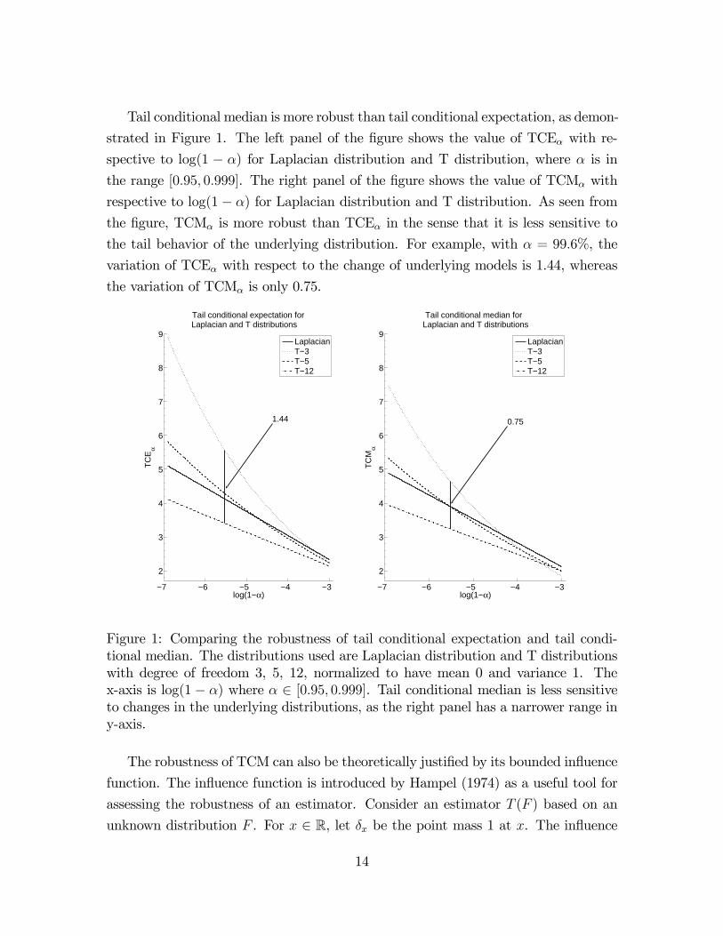
Tail conditional median is more robust than tail conditional expectation, as demon-

strated in Figure 1. The left panel of the figure shows the value of TCEα with re-

spective to log(1 − α) for Laplacian distribution and T distribution, where α is in

the range [0.95, 0.999]. The right panel of the figure shows the value of TCMα with

respective to log(1− α) for Laplacian distribution and T distribution. As seen from

the figure, TCMα is more robust than TCEα in the sense that it is less sensitive to

the tail behavior of the underlying distribution. For example, with α = 99.6%, the

variation of TCEα with respect to the change of underlying models is 1.44, whereas

the variation of TCMα is only 0.75.

−7 −6 −5 −4 −3

2

3

4

5

6

7

8

9

Tail conditional expectation for Laplacian and T distributions

log(1−α)

TC

Eα

LaplacianT−3T−5T−12

−7 −6 −5 −4 −3

2

3

4

5

6

7

8

9

Tail conditional median for Laplacian and T distributions

log(1−α)

TC

Mα

LaplacianT−3T−5T−12

1.44 0.75

Figure 1: Comparing the robustness of tail conditional expectation and tail condi-tional median. The distributions used are Laplacian distribution and T distributionswith degree of freedom 3, 5, 12, normalized to have mean 0 and variance 1. Thex-axis is log(1− α) where α ∈ [0.95, 0.999]. Tail conditional median is less sensitiveto changes in the underlying distributions, as the right panel has a narrower range iny-axis.

The robustness of TCM can also be theoretically justified by its bounded influence

function. The influence function is introduced by Hampel (1974) as a useful tool for

assessing the robustness of an estimator. Consider an estimator T (F ) based on an

unknown distribution F . For x ∈ R, let δx be the point mass 1 at x. The influence

14

function of the estimator T (F ) at x is defined by

IF (x, T, F ) = limε↓0

T ((1− ε)F + εδx)− T (F )

ε.

The influence function yields information about the rate of change of the estimator

T (F ) with respect to a contamination point x to the distribution F . An estimator T is

called bias robust at F , if its influence function is bounded, i.e., supx IF (x, T, F ) <∞.If the influence function of an estimator T (F ) is unbounded, then an outlier in the

data may cause problems. By simple calculation,6 TCE has an unbounded influence

function but TCM has a bounded influence function, which implies that TCM is more

robust than TCE with respect to outliers in the data.

4.4 Robust Risk Measures vs. Conservative Risk Measures

A risk measure is said to be more conservative than another one, if it generates higher

risk measurement than the other for the same underlying risk exposure. The use of

more conservative risk measures in external regulation is desirable from a regulator’s

viewpoint, since it generally increases the safety of the financial system (Of course,

risk measures should not be too conservative to retard the economic growth).

There is no contradiction between the robustness and the conservativeness of

external risk measures. Robustness addresses the issue of whether a risk measure can

be implemented consistently, so it is a requisite property of an external risk measure.

Conservativeness addresses the issue of how heavily an external risk measure should

be implemented to regulate the financial market, given that the external risk measure

can be implemented consistently. In other words, being more conservative is a further

desirable property of an external risk measure. An external risk measure should be

robust in the first place before one can consider the issue of how to implement it in

a conservative way.

For two reasons it is wrong to argue that TCE is more conservative than TCM

and hence is more suitable for external regulation:

(1) It is not true that TCE is more conservative than TCM. Indeed, it is not clear

which of the two risk measures gives higher risk measurement. Eling and Tibiletti

(2008) compare TCE and TCM for a set of capital market data, including the returns

of S&P 500 stocks, 1347 mutual funds and 205 hedge funds, and find that although

6See Appendix E.

15

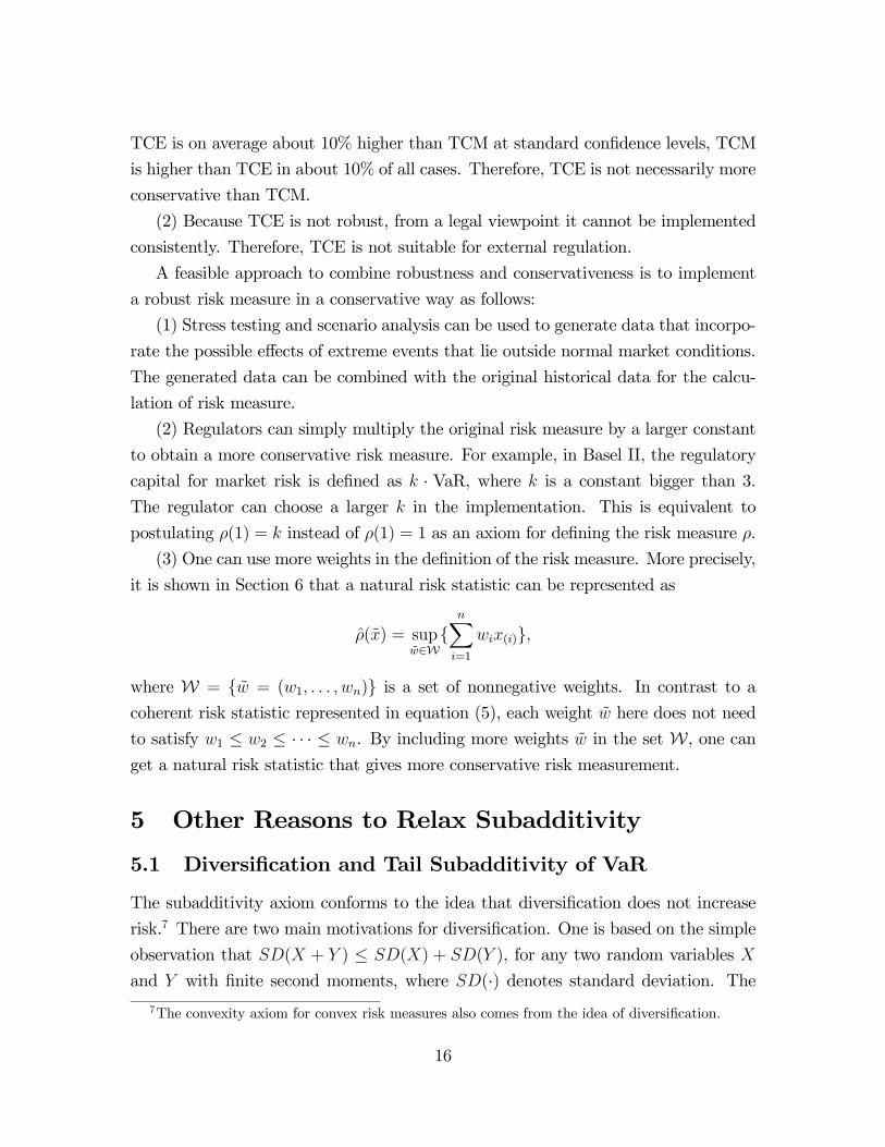
TCE is on average about 10% higher than TCM at standard confidence levels, TCM

is higher than TCE in about 10% of all cases. Therefore, TCE is not necessarily more

conservative than TCM.

(2) Because TCE is not robust, from a legal viewpoint it cannot be implemented

consistently. Therefore, TCE is not suitable for external regulation.

A feasible approach to combine robustness and conservativeness is to implement

a robust risk measure in a conservative way as follows:

(1) Stress testing and scenario analysis can be used to generate data that incorpo-

rate the possible effects of extreme events that lie outside normal market conditions.

The generated data can be combined with the original historical data for the calcu-

lation of risk measure.

(2) Regulators can simply multiply the original risk measure by a larger constant

to obtain a more conservative risk measure. For example, in Basel II, the regulatory

capital for market risk is defined as k · VaR, where k is a constant bigger than 3.The regulator can choose a larger k in the implementation. This is equivalent to

postulating ρ(1) = k instead of ρ(1) = 1 as an axiom for defining the risk measure ρ.

(3) One can use more weights in the definition of the risk measure. More precisely,

it is shown in Section 6 that a natural risk statistic can be represented as

ρ(x) = supw∈W

nXi=1

wix(i),

where W = w = (w1, . . . , wn) is a set of nonnegative weights. In contrast to acoherent risk statistic represented in equation (5), each weight w here does not need

to satisfy w1 ≤ w2 ≤ · · · ≤ wn. By including more weights w in the set W, one canget a natural risk statistic that gives more conservative risk measurement.

5 Other Reasons to Relax Subadditivity

5.1 Diversification and Tail Subadditivity of VaR

The subadditivity axiom conforms to the idea that diversification does not increase

risk.7 There are two main motivations for diversification. One is based on the simple

observation that SD(X + Y ) ≤ SD(X) + SD(Y ), for any two random variables X

and Y with finite second moments, where SD(·) denotes standard deviation. The7The convexity axiom for convex risk measures also comes from the idea of diversification.

16

other is based on expected utility theory. Samuelson (1967) shows that any investor

with a strictly concave utility function will uniformly diversify among independently

and identically distributed (i.i.d.) risks with finite second moments, i.e., the expected

utility of the uniformly diversified portfolio is larger than that of any other portfolio

constructed from these i.i.d. risks.8 Both of the two motivations require finiteness of

second moments of the risks.

Is diversification still preferable for risks with infinite second moments? The

answer can be no. Ibragimov and Walden (2006) show that diversification is not

preferable for unbounded extremely heavy-tailed distributions, in the sense that the

expected utility of the diversified portfolio is smaller than that of the undiversified

portfolio. They also show that, investors with certain S-shaped utility functions

would prefer non-diversification, even for bounded risks. A S-shaped utility function

is convex in the domain of losses. The convexity in the domain of losses is supported

by experimental results and prospect theory (Kahneman and Tversky, 1979; Tversky

and Kahneman, 1992), which is an important alternative to expected utility theory.

See Section 5.3 for more discussion on prospect theory.

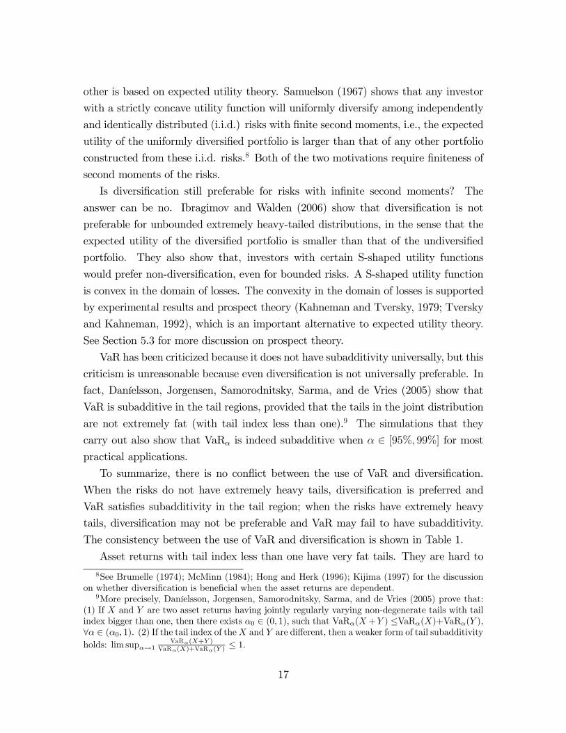
VaR has been criticized because it does not have subadditivity universally, but this

criticism is unreasonable because even diversification is not universally preferable. In

fact, Daníelsson, Jorgensen, Samorodnitsky, Sarma, and de Vries (2005) show that

VaR is subadditive in the tail regions, provided that the tails in the joint distribution

are not extremely fat (with tail index less than one).9 The simulations that they

carry out also show that VaRα is indeed subadditive when α ∈ [95%, 99%] for mostpractical applications.

To summarize, there is no conflict between the use of VaR and diversification.

When the risks do not have extremely heavy tails, diversification is preferred and

VaR satisfies subadditivity in the tail region; when the risks have extremely heavy

tails, diversification may not be preferable and VaR may fail to have subadditivity.

The consistency between the use of VaR and diversification is shown in Table 1.

Asset returns with tail index less than one have very fat tails. They are hard to

8See Brumelle (1974); McMinn (1984); Hong and Herk (1996); Kijima (1997) for the discussionon whether diversification is beneficial when the asset returns are dependent.

9More precisely, Daníelsson, Jorgensen, Samorodnitsky, Sarma, and de Vries (2005) prove that:(1) If X and Y are two asset returns having jointly regularly varying non-degenerate tails with tailindex bigger than one, then there exists α0 ∈ (0, 1), such that VaRα(X+Y ) ≤VaRα(X)+VaRα(Y ),∀α ∈ (α0, 1). (2) If the tail index of theX and Y are different, then a weaker form of tail subadditivityholds: lim supα→1

VaRα(X+Y )VaRα(X)+VaRα(Y )

≤ 1.

17

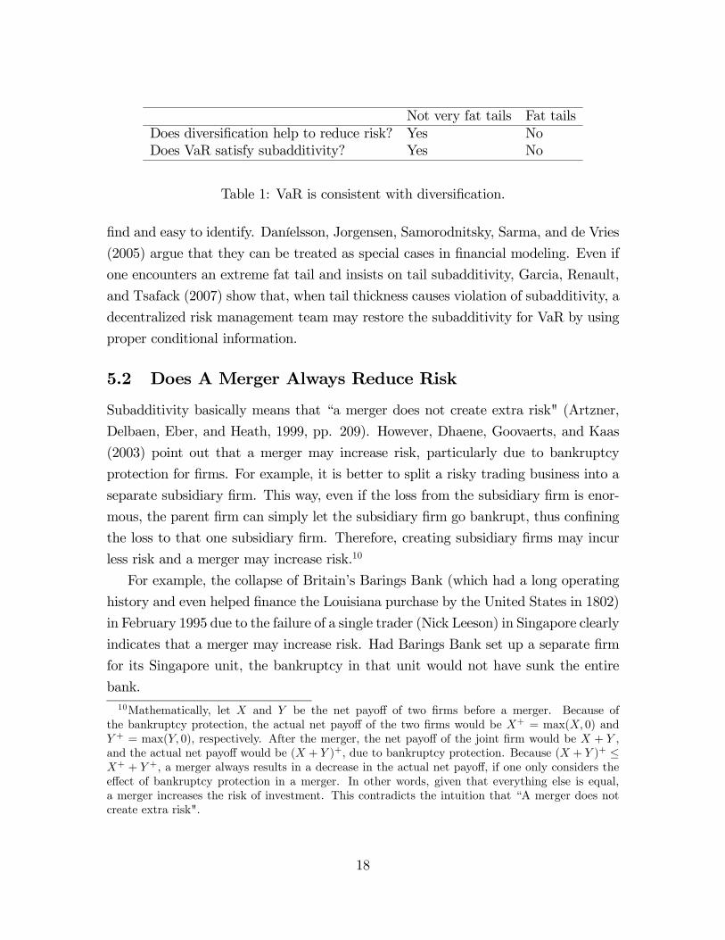
Not very fat tails Fat tailsDoes diversification help to reduce risk? Yes NoDoes VaR satisfy subadditivity? Yes No

Table 1: VaR is consistent with diversification.

find and easy to identify. Daníelsson, Jorgensen, Samorodnitsky, Sarma, and de Vries

(2005) argue that they can be treated as special cases in financial modeling. Even if

one encounters an extreme fat tail and insists on tail subadditivity, Garcia, Renault,

and Tsafack (2007) show that, when tail thickness causes violation of subadditivity, a

decentralized risk management team may restore the subadditivity for VaR by using

proper conditional information.

5.2 Does A Merger Always Reduce Risk

Subadditivity basically means that “a merger does not create extra risk" (Artzner,

Delbaen, Eber, and Heath, 1999, pp. 209). However, Dhaene, Goovaerts, and Kaas

(2003) point out that a merger may increase risk, particularly due to bankruptcy

protection for firms. For example, it is better to split a risky trading business into a

separate subsidiary firm. This way, even if the loss from the subsidiary firm is enor-

mous, the parent firm can simply let the subsidiary firm go bankrupt, thus confining

the loss to that one subsidiary firm. Therefore, creating subsidiary firms may incur

less risk and a merger may increase risk.10

For example, the collapse of Britain’s Barings Bank (which had a long operating

history and even helped finance the Louisiana purchase by the United States in 1802)

in February 1995 due to the failure of a single trader (Nick Leeson) in Singapore clearly

indicates that a merger may increase risk. Had Barings Bank set up a separate firm

for its Singapore unit, the bankruptcy in that unit would not have sunk the entire

bank.10Mathematically, let X and Y be the net payoff of two firms before a merger. Because of

the bankruptcy protection, the actual net payoff of the two firms would be X+ = max(X, 0) andY + = max(Y, 0), respectively. After the merger, the net payoff of the joint firm would be X + Y ,and the actual net payoff would be (X + Y )+, due to bankruptcy protection. Because (X + Y )+ ≤X+ + Y +, a merger always results in a decrease in the actual net payoff, if one only considers theeffect of bankruptcy protection in a merger. In other words, given that everything else is equal,a merger increases the risk of investment. This contradicts the intuition that “A merger does notcreate extra risk".

18

In addition, there is little empirical evidence supporting the argument that “a

merger does not create extra risk”. Indeed, in practice, the credit rating agencies,

such as Moody’s and Standard & Poor’s, do not upgrade a firm’s credit rating because

of a merger. On the contrary, the credit rating of the joint firmmay be lowered shortly

after the merger of two firms; the recent merger of Bank of America and Merrill Lynch

is such an example.

5.3 Psychological Theory of Uncertainty and Risk

Risk measures have a close connection with the psychological theory of people’s pref-

erences of uncertainties and risks. Kahneman and Tversky (1979) and Tversky and

Kahneman (1992) point out that people’s choices under risky prospects are incon-

sistent with the basic tenets of expected utility theory and propose an alternative

model, called prospect theory, which can explain a variety of preference anomalies in-

cluding the Allais and Ellsberg paradoxes. The axiomatic analysis of prospect theory

is presented in Tversky and Kahneman (1992) and extended in Wakker and Tversky

(1993). Many other people have studied alternative models to expected utility theory,

such as Quiggin (1982), Schmeidler (1986), Yaari (1987), Schmeidler (1989), and so

on. These models are referred to as “anticipated utility theory", “rank-dependent

models", “cumulative utility theory", etc.

Prospect theory implies fourfold pattern of risk attitudes: people are risk averse

for gains with high probability and losses with low probability; and people are risk

seeking for gains with low probability and losses with high probability. Prospect

theory postulates that: (1) The value function (utility function) is normally concave

for gains, convex for losses, and is steeper for losses than for gains. (2) People evaluate

uncertain prospects using “decision weights” that are nonlinear transformation of

probabilities and can be viewed as distorted probabilities.

Schmeidler (1989) points out that risk preferences for comonotonic random vari-

ables are easier to justify than those for arbitrary random variables and accordingly

relaxes the independence axiom in expected utility theory to the comonotonic inde-

pendence axiom that applies only to comonotonic random variables. Tversky and

Kahneman (1992) and Wakker and Tversky (1993) also find that prospect theory

is characterized by the axioms that impose conditions only on comonotonic random

variables and are thus less restrictive than their counterparts in expected utility the-

ory.

19

There are simple examples showing that risk associated with non-comonotonic

random variables can violate subadditivity, because people are risk seeking instead

of risk averse in choices between probable and sure losses, as implied by prospect

theory.11 12

Motivated by the prospect theory, we think it may be appropriate to relax the

subadditivity to comonotonic subadditivity. In other words, we impose ρ(X + Y ) ≤ρ(X)+ ρ(Y ) only for comonotonic random variables X and Y when defining the new

risk measures.

6 Main Results: Natural Risk Statistics and TheirAxiomatic Representations

Suppose we have a collection of data x = (x1, x2, . . . , xn) ∈ Rn related to a random

loss X, which can be discrete or continuous. x can be a set of historical observations,

or a set of simulated data generated according to a well-defined procedure or model,

or a mixture of historical and simulated data. To measure risk from the data x, we

define a risk statistic ρ to be a mapping from Rn to R. A risk statistic is a data-based11Suppose there is an urn that contains 50 black balls and 50 red balls. Randomly draw a ball

from the urn. Let B be the position of losing $10,000 in the event that the ball is black, andR be the position of losing $10,000 in the event that the ball is red. Obviously, B and R bearthe same amount of risk, i.e., ρ(B) = ρ(R). Let S be the event of losing $5,000 for sure, thenρ(S) = 5, 000. According to prospect theory, people are risk seeking in choices between probableand sure losses, i.e., most people would prefer a larger loss with a substantial probability to a sureloss. Therefore, most people would prefer position B to position S (see problem 12 on pp. 273in Kahneman and Tversky (1979), and table 3 on pp. 307 in Tversky and Kahneman (1992)).In other words, we have ρ(B) = ρ(R) < ρ(S) = 5, 000. On the other hand, since the positionB + R corresponds to a sure loss of $10,000, we have ρ(B + R) = 10, 000. Combining together wehave ρ(B) + ρ(R) < 5, 000 + 5, 000 = 10, 000 = ρ(B + R), violating the subadditivity. Clearly therandom losses associated with B and R are not comonotonic. Therefore, this example shows thatrisk associated with non-comonotonic random variables may violate subadditivity.12Even in terms of expected utility theory, it is not clear whether a risk measure should be super-

additive or subadditive for independent random variables. For instance, Eeckhoudt and Schlesinger(2006) link the sign of utility functions to risk preferences. Let u(4) be the fourth derivative ofan utility function u. They prove that u(4) ≤ 0 if and only if E(u(x + 1 + 2)) + E(u(x)) ≤E(u(x + 1)) + E(u(x + 2)), for any x ∈ R and any independent risks 1 and 2 satisfyingE( 1) = E( 2) = 0. This result can be interpreted as follows. Suppose the owner of two sub-sidiary firms, each of which has initial wealth x, faces the problem of assigning two projects to thetwo firms. The net payoffs of the two projects are 1 and 2, respectively. The result suggests that,whether the owner prefers to assign both projects to a single firm or prefers to assign one project toeach firm depends on the sign of the fourth derivative of his utility function. Because comonotonicrandom variables are generally not independent, we shall impose subadditivity only for comonotonicrandom variables to avoid the issue of possible superadditivity for independent random variables.

20

risk measure.

In this section, we will define and fully characterize the new data-based risk mea-

sure, which we call the natural risk statistic, through two sets of axioms and two

representations.

6.1 The First Representation

At first, we postulate the following axioms for a risk statistic ρ.

Axiom C1. Positive homogeneity and translation invariance:

ρ(ax+ b1) = aρ(x) + b, ∀x ∈ Rn, a ≥ 0, b ∈ R,

where 1 = (1, 1, ..., 1)T ∈ Rn.

Axiom C2. Monotonicity: ρ(x) ≤ ρ(y), if x ≤ y, where x ≤ y means xi ≤ yi, i =

1, . . . , n.

The two axioms above have been proposed for coherent risk measures. Here we

simply adapt them to the case of risk statistics. Note that Axiom C1 yields

ρ(0 · 1) = 0, ρ(b1) = b, b ∈ R,

and Axioms C1 and C2 imply ρ is continuous.13

Axiom C3. Comonotonic subadditivity:

ρ(x+ y) ≤ ρ(x) + ρ(y), if x and y are comonotonic,

where x and y are comonotonic if and only if (xi − xj)(yi − yj) ≥ 0, for any i 6= j.

In Axiom C3 we relax the subadditivity requirement in coherent risk measures so

that the axiom is only enforced for comonotonic random variables. This also relaxes

the comonotonic additivity requirement in insurance risk measures. Comonotonic

subadditivity is consistent with prospect theory, as we explained in Section 5.3.

Axiom C4. Permutation invariance:

ρ((x1, . . . , xn)) = ρ((xi1 , . . . , xin))

for any permutation (i1, . . . , in) of (1, 2, . . . , n).

13Indeed, suppose ρ satisfies Axiom C1 and C2. Then for any x ∈ Rn, ε > 0, and y satisfying|yi − xi| < ε, i = 1, . . . , n, we have x − ε1 < y < x + ε1. By the monotonicity in Axiom C2,we have ρ(x − ε1) ≤ ρ(y) ≤ ρ(x + ε1). Applying Axiom C1, the inequality further becomesρ(x)− ε ≤ ρ(y) ≤ ρ(x) + ε, which establishes the continuity of ρ.

21

This axiom can be considered as the counterpart of the law invariance AxiomA4 in

terms of data. It means that if two data x and y have the same empirical distribution,

i.e., the same order statistics, then x and y should give the same measurement of risk.

Definition 1. A risk statistic ρ : Rn → R is called a natural risk statistic if itsatisfies Axiom C1-C4.

The following representation theorem for natural risk statistics is one of the main

results of this paper.

Theorem 1 Let x(1), ..., x(n) be the order statistics of the data x with x(n) being the

largest.

(I) For an arbitrarily given set of weights W = w = (w1, . . . , wn) ⊂ Rn with

each w ∈W satisfyingPn

i=1wi = 1 and wi ≥ 0 for i = 1, . . . , n, the risk statistic

ρ(x) , supw∈W

nXi=1

wix(i), ∀x ∈ Rn (7)

is a natural risk statistic.

(II) If ρ is a natural risk statistic, then there exists a set of weights W = w =

(w1, . . . , wn) ⊂ Rn with each w ∈ W satisfyingPn

i=1wi = 1 and wi ≥ 0 for i =1, . . . , n, such that

ρ(x) = supw∈W

nXi=1

wix(i), ∀x ∈ Rn. (8)

Proof. See Appendix A. Q.E.D.

The main difficulty in proving Theorem 1 lies in part (II). Axiom C3 implies

that the functional ρ satisfies subadditivity on comonotonic sets of Rn, for example,

on the set B = y ∈ Rn | y1 ≤ y2 ≤ · · · ≤ yn. However, unlike in the case ofcoherent risk measures, the existence of a set of weights W such that (8) holds does

not follow easily from the proof in Huber (1981). The main difference here is that

the comonotonic set B is not an open set in Rn. The boundary points do not have

as nice properties as the interior points. We have to treat boundary points with

more efforts. In particular, one should be very cautious when using the results of

separating hyperplanes. Furthermore, we have to spend some effort showing that

wi ≥ 0 for i = 1, . . . , n.14

14Utilizing convex duality theory, Ahmed, Filipovic, and Svindland (2008) provide alternativeshorter proofs for Theorem 1 and Theorem 4 after seeing the first version of this paper.

22

Each weight w in the set W in equation (7) represents a scenario, so natural risk

statistics can incorporate scenario analysis by putting different weights on the order

statistics. In addition, since estimating VaR from data is equivalent to calculating

weighted average of the order statistics, Theorem 1 shows that natural risk statistics

include VaR along with scenario analysis as a special case.

6.2 The Second Representation via Acceptance Sets

The natural risk statistics can also be characterized via acceptance sets as in the case

of coherent risk measures. More precisely, a statistical acceptance set is a subset of

Rn that includes all the data that are considered acceptable by a regulator. Given a

statistical acceptance set A ∈ Rn, the risk statistic ρA associated with A is defined

to be the minimal amount of risk-free investment that has to be added to the original

position in order for the resulting position to be acceptable, or in mathematical form

ρA(x) = infm | x−m1 ∈ A, ∀x ∈ Rn. (9)

On the other hand, given a risk statistic ρ, one can define the statistical acceptance

set associated with ρ by

Aρ = x ∈ Rn | ρ(x) ≤ 0. (10)

Thus, one can go from a risk measure to an acceptance set, and vice versa.

We shall postulate the following axioms for statistical acceptance set A:Axiom D1. The statistical acceptance set A contains Rn

− where Rn− = x ∈ Rn |

xi ≤ 0, i = 1, . . . , n.Axiom D2. The statistical acceptance setA does not intersect the set Rn

++ where

Rn++ = x ∈ Rn | xi > 0, i = 1, . . . , n.Axiom D3. If x and y are comonotonic and x ∈ A, y ∈ A, then λx+(1−λ)y ∈ A,

for ∀λ ∈ [0, 1].Axiom D4. The statistical acceptance set A is positively homogeneous, i.e., if

x ∈ A, then λx ∈ A for all λ ≥ 0.Axiom D5. If x ≤ y and y ∈ A, then x ∈ A.Axiom D6. If x ∈ A, then (xi1, . . . , xin) ∈ A for any permutation (i1, . . . , in) of

(1, 2, . . . , n).

We will show that a natural risk statistic and a statistical acceptance set satisfying

Axiom D1-D6 are mutually representable. More precisely, we have the following

theorem:

23

Theorem 2 (I) If ρ is a natural risk statistic, then the statistical acceptance set Aρ

is closed and satisfies Axiom D1-D6.

(II) If a statistical acceptance set A satisfies Axiom D1-D6, then the risk statisticρA is a natural risk statistic.

(III) If ρ is a natural risk statistic, then ρ = ρAρ.

(IV) If a statistical acceptance set D satisfies Axiom D1-D6, then AρD = D, theclosure of D.

Proof. See Appendix B. Q.E.D.

7 Comparison with Coherent and Insurance RiskMeasures

7.1 Comparison with Coherent Risk Measures

To compare natural risk statistics with coherent risk measures in a formal manner,

we first define the coherent risk statistics, the data-based versions of coherent risk

measures.

Definition 2. A risk statistic ρ : Rn → R is called a coherent risk statistic, if itsatisfies Axiom C1, C2 and the following Axiom E3:

Axiom E3. Subadditivity: ρ(x+ y) ≤ ρ(x) + ρ(y), for any x, y ∈ Rn.

We have the following representation theorem for coherent risk statistics.

Theorem 3 A risk statistic ρ is a coherent risk statistic if and only if there exists aset of weights W = w = (w1, . . . , wn) ⊂ Rn with each w ∈W satisfying

Pni=1wi =

1 and wi ≥ 0, i = 1, . . . , n, such that

ρ(x) = supw∈W

nXi=1

wixi, ∀x ∈ Rn. (11)

Proof. The proof for the “if” part is trivial. To prove the “only if” part,

suppose ρ is a coherent risk statistic. Let Θ = θ1, . . . , θn be an arbitrary setwith n elements. Let H be the set of all the subsets of Θ. Let Z be the set of

all real-valued random variables defined on (Θ,H). Define a functional E∗ on Z:E∗(Z) , ρ(Z(θ1), Z(θ2), . . . , Z(θn)). Then E∗(·) is monotone, positively affinely ho-mogeneous, and subadditive in the sense defined in equations (2.7), (2.8) and (2.9)

24

at Chapter 10 of Huber (1981). Then the result follows by applying Proposition 2.1

at page 254 of Huber (1981) to E∗. Q.E.D.

Natural risk statistics require the permutation invariance, which is not required

by coherent risk statistics. To have a complete comparison between natural risk

statistics and coherent risk measures, we consider the following law-invariant coherent

risk statistics, which are the counterparts of law-invariant coherent risk measures.

Definition 3. A risk statistic ρ : Rn → R is called a law-invariant coherent riskstatistic, if it satisfies Axiom C1, C2, C4 and E3.

We have the following representation theorem for law-invariant coherent risk sta-

tistics.

Theorem 4 Let x(1), ..., x(n) be the order statistics of the data x with x(n) being the

largest.

(I) For an arbitrarily given set of weights W = w = (w1, . . . , wn) ⊂ Rn with

each w ∈W satisfying

nXi=1

wi = 1, (12)

wi ≥ 0, i = 1, . . . , n, (13)

w1 ≤ w2 ≤ . . . ≤ wn, (14)

the risk statistic

ρ(x) , supw∈W

nXi=1

wix(i), ∀x ∈ Rn (15)

is a law-invariant coherent risk statistic.

(II) If ρ is a law-invariant coherent risk statistic, then there exists a set of weights

W = w = (w1, . . . , wn) ⊂ Rn with each w ∈W satisfying (12), (13) and (14), such

that

ρ(x) = supw∈W

nXi=1

wix(i), ∀x ∈ Rn. (16)

Proof. See Appendix C. Q.E.D.

By Theorem 3 and Theorem 4, we see the main differences between natural risk

statistics and coherent risk measures:

(1) A natural risk statistic is the supremum of a set of L-statistics (a L-statistic is

a weighted average of order statistics), while a coherent risk statistic is a supremum

25

of a weighted sample average. There is no simple linear function that can transform

a L-statistic to a weighted sample average.

(2) Although VaR is not a coherent risk statistic, VaR is a natural risk statistic. In

other words, though being simple, VaR is not without justification, as it also satisfies

a reasonable set of axioms.

(3) A law-invariant coherent risk statistic is the supremum of a set of L-statistics

with increasing weights. Hence, if one assigns larger weights to larger observations,

a natural risk statistic becomes a law invariant coherent risk statistic. However,

assigning larger weights to larger observations is not robust. Therefore, coherent risk

measures are in general not robust.

7.2 Comparison with Insurance Risk Measures

Similarly, we can define the insurance risk statistics, the data-based versions of insur-

ance risk measures, as follows:

Definition 3. A risk statistic ρ : Rn → R is called an insurance risk statistic, ifit satisfies the following Axiom F1-F4.

Axiom F1. Permutation invariance: the same as Axiom C4.

Axiom F2. Monotonicity: ρ(x) ≤ ρ(y), if x ≤ y.

Axiom F3. Comonotonic additivity: ρ(x + y) = ρ(x) + ρ(y), if x and y are

comonotonic.

Axiom F4. Scale normalization: ρ(1) = 1.We have the following representation theorem for insurance risk statistics.

Theorem 5 Let x(1), ..., x(n) be the order statistics of the data x with x(n) being the

largest, then ρ is an insurance risk statistic if and only if there exists a single weight

w = (w1, . . . , wn) with wi ≥ 0 for i = 1, . . . , n andPn

i=1wi = 1, such that

ρ(x) =nXi=1

wix(i), ∀x ∈ Rn. (17)

Proof. See Appendix D. Q.E.D.

Comparing (8) and (17), we see that a natural risk statistic is the supremum of

a set of L-statistics, while an insurance risk statistic is just one L-statistic. There-

fore, insurance risk statistics cannot incorporate different scenarios. On the other

hand, each weight w = (w1, . . . , wn) in a natural risk statistic can be considered as

26

a “scenario" in which (subjective or objective) evaluation of the importance of each

ordered observation is specified. Hence, nature risk statistics incorporate the idea of

evaluating risk under different scenarios, so do coherent risk measures.

The following counterexample shows that if one incorporates different scenarios,

then the comonotonic additivity may not hold, as the strict comonotonic subadditivity

may prevail.

A counterexample: consider a natural risk statistic defined by

ρ(x) = max(0.5x(1) + 0.5x(2), 0.72x(1) + 0.08x(2) + 0.2x(3)), ∀x ∈ R3.

Let y = (3, 2, 4) and z = (9, 4, 16). By simple calculation we have

ρ(y + z) = 9.28 < ρ(y) + ρ(z) = 2.5 + 6.8 = 9.3,

even though y and z are comonotonic. Therefore, the comonotonic additivity fails, and

this natural risk statistic is not an insurance risk statistic. In summary, insurance risk

statistic cannot incorporate those two simple scenarios with weights being (0.5, 0.5, 0)

and (0.72, 0.08, 0.2).

7.3 Comparison from the Viewpoint of Computation

We compare the computation of TCE and TCM in two aspects: whether it is easy

to compute a risk measure from a regulator’s viewpoint, and whether it is easy to

incorporate a risk measure into portfolio optimization from an individual bank’s view-

point. First, the computation of TCM is at least as easy as the computation of TCE,

since the former only involves the computation of quantile. Second, it is easier to do

portfolio optimization with respect to TCE than to TCM, as the expectation leads

to convexity in optimization. However, we should point out that doing optimization

with respect to median is a classical problem in robust statistics, and recently there

are good algorithms designed for portfolio optimization under both CVaR and VaR

constraints (see Rockafellar and Uryasev, 2000, 2002). Furthermore, from the regula-

tor’s viewpoint, it is a first priority to find a good robust risk measure for the purpose

of legal implementation. How to achieve better profits via portfolio optimization,

under the risk measure constraints imposed by governmental regulations, should be

a matter left for investors not the regulator.

27

8 Some Counterexamples Showing that Tail Con-ditional Median Satisfies Subadditivity

In the existing literature, some examples are used to show that VaR does not satisfy

subadditivity at certain level α. However, if one considers TCM at the same level α,

or equivalently considers VaR at a higher level, the problem of non-subadditivity of

VaR disappears.

Example 1. The VaRs in the example on page 216 of Artzner, Delbaen, Eber,and Heath (1999) are not correctly calculated. Actually in that example, the 1%

VaR15 of two options A and two options B are 2u and 2l respectively, instead of −2uand −2l. And the 1% VaR of A+B is u+ l, instead of 100− l − u. Therefore, VaR

satisfies subadditivity in that example.

Example 2. The example on page 217 of Artzner, Delbaen, Eber, and Heath(1999) shows that the 10% VaR does not satisfy subadditivity for X1 and X2. How-

ever, the 10% tail conditional median (or equivalently 5% VaR) satisfies subadditiv-

ity! Actually, the 5% VaR of X1 and X2 are both equal to 1. By simple calculation,

P (X1 + X2 ≤ −2) = 0.005 < 0.05, which implies that the 5% VaR of X1 + X2 is

strictly less than 2.

Example 3. The example in section 2.1 of Dunkel and Weber (2007) shows thatthe 99% VaR of L1 and L2 are equal, although apparently L2 is much more risky than

L1. However, tail conditional median at 99% level (or 99.5% VaR), of L1 is equal to

1010, which is much larger than 1, tail conditional median at 99% level (99.5% VaR)

of L2. In other words, if one looks at tail conditional median at 99% level, one can

correctly compare the risk of the two portfolios.

9 Conclusion

We propose new, data-based, risk measures, called natural risk statistics, that are

characterized by a new set of axioms. The new axioms only require subadditivity

for comonotonic random variables, thus relaxing the subadditivity for all random

variables in coherent risk measures, and relaxing the comonotonic additivity in insur-

ance risk measures. The relaxation is consistent with prospect theory in psychology.

15In Artzner, Delbaen, Eber, and Heath (1999), VaR is defined as VaR(X) = − infx | P (X ≤x) > α, where X = −L representing the net worth of a position. In other words, VaR at level α inArtzner, Delbaen, Eber, and Heath (1999) corresponds to VaR at level 1− α in this paper.

28

Comparing to existing risk measures, natural risk statistics include tail conditional

median, which is more robust than tail conditional expectation suggested by coher-

ent risk measures; and, unlike insurance risk measures, natural risk statistics can

also incorporate scenario analysis. Natural risk statistics include VaR (with scenario

analysis) as a special case and therefore show that VaR, though simple, is not irra-

tional.

We emphasize that the objectives of risk measures are very relevant for our dis-

cussion. In particular, some risk measures may be suitable for internal management

but not for external regulation, and vice versa. For example, coherent and convex

risk measures may be good for internal risk measurement, as there are connections

between these risk measures and subjective prices in incomplete markets for market

makers (see, e.g., the connections between coherent and convex risk measures and

good deal bounds in Jaschke and Küchler, 2001; Staum, 2004). However, as we point

out, for external risk measures one may prefer a different set of properties, including

consistency in implementation which means robustness.

A Proof of Theorem 1

The proof relies on the following two lemmas, which depend heavily on the properties

of the interior points of the set B = y ∈ Rn | y1 ≤ y2 ≤ · · · ≤ yn and hence are onlytrue for the interior points. The results for boundary points will be obtained by ap-

proximating the boundary points by the interior points, and by employing continuity

and uniform convergence.

Lemma 1 Let B = y ∈ Rn | y1 ≤ y2 ≤ · · · ≤ yn, and denote Bo to be the

interior of B. For any fixed z = (z1, . . . , zn) ∈ Bo and any ρ satisfying Axiom C1-C4

and ρ(z) = 1 there exists a weight w = (w1, . . . , wn) such that the linear functional

λ(x) ,Pn

i=1wixi satisfies

λ(z) = 1, (18)

λ(x) < 1 for all x such that x ∈ B and ρ(x) < 1. (19)

Proof. Let U = x | ρ(x) < 1 ∩ B. For any x, y ∈ B, x and y are comonotonic.

Then Axiom C1 and C3 imply that U is convex, and, therefore, the closure U of U is

also convex.

29

For any ε > 0, since ρ(z − ε1) = ρ(z)− ε = 1− ε < 1, it follows that z − ε1 ∈ U .

Since z − ε1 tends to z as ε ↓ 0, we know that z is a boundary point of U because

ρ(z) = 1. Therefore, there exists a supporting hyperplane for U at z, i.e., there

exists a nonzero vector w = (w1, . . . , wn) ∈ Rn such that λ(x) ,Pn

i=1wixi satisfies

λ(x) ≤ λ(z) for all x ∈ U . In particular, we have

λ(x) ≤ λ(z), ∀x ∈ U. (20)

We shall show that the strict inequality holds in (20). Suppose, by contradiction,

that there exists x0 ∈ U such that λ(x0) = λ(z). For any α ∈ (0, 1), let xα =αz + (1− α)x0. Then we have

λ(xα) = αλ(z) + (1− α)λ(x0) = λ(z) (21)

In addition, since z and x0 are comonotonic (as they all belong to B) we have

ρ(xα) ≤ αρ(z) + (1− α)ρ(x0) < α+ (1− α) = 1, ∀α ∈ (0, 1). (22)

Since z ∈ Bo, it follows that there exists α0 ∈ (0, 1) such that xα0 is also an interiorpoint of B. Hence, for all small enough ε > 0,

xα0 + εw ∈ B. (23)

With wmax = max(w1, w2, ..., wn), we have xα0 + εw ≤ xα0 + εwmax1. Thus, the

monotonicity in Axiom C2 and translation invariance in Axiom C1 yield

ρ(xα0 + εw) ≤ ρ(xα0 + εwmax1) = ρ(xα0) + εwmax. (24)

Since ρ(xα0) < 1 via (22), we have by (24) and (23) that for all small enough ε > 0,

ρ(xα0+εw) < 1, xα0+εw ∈ U . Hence, (20) implies λ(xα0+εw) ≤ λ(z). However, we

have, by (21), an opposite inequality λ(xα0 + εw) = λ(xα0) + ε|w|2 > λ(xα0) = λ(z),

leading to a contradiction. In summary, we have shown that

λ(x) < λ(z),∀x ∈ U. (25)

Since ρ(0) = 0, we have 0 ∈ U . Letting x = 0 in (25) yields λ(z) > 0, so we can

re-scale w such that λ(z) = 1 = ρ(z). Thus, (25) becomes λ(x) < 1 for all x such

that x ∈ B and ρ(x) < 1, from which (19) holds. Q.E.D.

30

Lemma 2 Let B = y ∈ Rn | y1 ≤ y2 ≤ · · · ≤ yn, and denote Bo to be the interior

of B. For any fixed z = (z1, . . . , zn) ∈ Bo and any ρ satisfying Axiom C1-C4, there

exists a weight w = (w1, . . . , wn) such thatnXi=1

wi = 1, (26)

wi ≥ 0, i = 1, . . . , n, (27)

ρ(x) ≥nXi=1

wixi, for ∀x ∈ B, and ρ(z) =nXi=1

wizi. (28)

Proof. We will show this by considering three cases.

Case 1: ρ(z) = 1.

From Lemma 1, there exists a weight w = (w1, . . . , wn) such that the linear

functional λ(x) ,Pn

i=1wixi satisfies (18) and (19).

First we prove that w satisfies (26). For this, it is sufficient to show that λ(1) =Pni=1wi = 1. To this end, first note that for any c < 1 Axiom C1 implies ρ(c1) = c <

1. Thus, (19) implies λ(c1) < 1, and, by continuity of λ, we obtain that λ(1) ≤ 1.Secondly, for any c > 1, Axiom C1 implies ρ(2z − c1) = 2ρ(z)− c = 2− c < 1. Then

it follows from (19) and (18) that 1 > λ(2z − c1) = 2λ(z) − cλ(1) = 2 − cλ(1), i.e.

λ(1) > 1/c for any c > 1. So λ(1) ≥ 1, and w satisfies (26).

Next, we will prove that w satisfies (27). Let ek = (0, . . . , 0, 1, 0, . . . , 0) be the

k-th standard basis of Rn. Then wk = λ(ek). Since z ∈ Bo, there exists δ > 0 such

that z − δek ∈ B. For any ε > 0, we have

ρ(z − δek − ε1) = ρ(z − δek)− ε ≤ ρ(z)− ε = 1− ε < 1,

where the inequality follows from the monotonicity in Axiom C2. Then (19) and (18)

implies

1 > λ(z − δek − ε1) = λ(z)− δλ(ek)− ελ(1) = 1− ε− δλ(ek).

Hence wk = λ(ek) > −ε/δ, and the conclusion follows by letting ε go to 0.Finally, we will prove that w satisfies (28). It follows from Axiom C1 and (19)

that

∀c > 0, λ(x) < c, for all x such that x ∈ B and ρ(x) < c. (29)

For any c ≤ 0, we choose b > 0 such that b+ c > 0. Then by (29), we have

λ(x+ b1) < c+ b, for all x such that x ∈ B and ρ(x+ b1) < c+ b.

31

Since λ(x+ b1) = λ(x) + bλ(1) = λ(x) + b and ρ(x+ b1) = ρ(x) + b we have

∀c ≤ 0, λ(x) < c, for all x such that x ∈ B and ρ(x) < c. (30)

It follows from (29) and (30) that ρ(x) ≥ λ(x), for all x ∈ B, which in combinationwith ρ(z) = λ(z) = 1 completes the proof of (28).

Case 2: ρ(z) 6= 1 and ρ(z) > 0.

Since ρ³

1ρ(z)

z´= 1 and 1

ρ(z)z is still an interior point of B, it follows from the result

proved in Case 1 that there exists a linear functional λ(x) ,Pn

i=1wixi, with w =

(w1, . . . , wn) satisfying (26), (27) and ρ(x) ≥ λ(x), ∀x ∈ B, and ρ³

1ρ(z)

z´= λ

³1

ρ(z)z´,

or equivalently ρ(x) ≥ λ(x),∀x ∈ B, and ρ(z) = λ(z). Thus, w also satisfies (28).

Case 3: ρ(z) ≤ 0.Choose b > 0 such that ρ(z + b1) > 0. Since z + b1 is an interior point of B, it

follows from the result proved in Case 2 that there exists a linear functional λ(x) ,Pni=1wixi with w = (w1, . . . , wn) satisfying (26), (27) and ρ(x) ≥ λ(x),∀x ∈ B,

and ρ(z + b1) = λ(z + b1), or equivalently ρ(x) ≥ λ(x),∀x ∈ B, and ρ(z) = λ(z).

Thus, w also satisfies (28). Q.E.D.

The proof for Theorem 1 is as follows.

Proof. (1) The proof of part (I). Suppose ρ is defined by (7), then obviously ρ

satisfies Axiom C1 and C4.

To check AxiomC2, write (y(1), y(2), . . . , y(n)) = (yi1 , yi2 , . . . , yin), where (i1, . . . , in)

is a permutation of (1, . . . , n). Then for any x ≤ y, we have

y(k) ≥ maxyij , j = 1, . . . , k ≥ maxxij , j = 1, . . . , k ≥ x(k), 1 ≤ k ≤ n,

which implies that ρ satisfies Axiom C2 because

ρ(y) = supw∈W

nXi=1

wiy(i) ≥ supw∈W

nXi=1

wix(i) = ρ(x).

To check Axiom C3, note that if x and y are comonotonic, then there exists a

permutation (i1, . . . , in) of (1, . . . , n) such that xi1 ≤ xi2 ≤ . . . ≤ xin and yi1 ≤ yi2 ≤. . . ≤ yin. Hence, we have (x+ y)(i) = x(i) + y(i), i = 1, ..., n. Therefore,

ρ(x+ y) = supw∈W

nXi=1

wi(x+ y)(i) = supw∈W

nXi=1

wi(x(i) + y(i))

≤ supw∈W

nXi=1

wix(i)+ supw∈W

nXi=1

wiy(i) = ρ(x) + ρ(y),

32

which implies that ρ satisfies Axiom C3.

(2) The proof of part (II). By Axiom C4, we only need to show that there exists a

set of weights W = w = (w1, . . . , wn) ⊂ Rn with each w ∈W satisfyingPn

i=1wi =

1 and wi ≥ 0, ∀1 ≤ i ≤ n, such that ρ(x) = supw∈WPn

i=1wixi, ∀x ∈ B, whereB = y ∈ Rn | y1 ≤ y2 ≤ · · · ≤ yn.By Lemma 2, for any point y ∈ Bo, there exists a weight w(y) satisfying (26), (27)

and (28). Therefore, we can take the collection of such weights as W = w(y) | y ∈Bo. Then from (28), for any fixed x ∈ Bo we have ρ(x) ≥

Pni=1w

(y)i xi, ∀y ∈ Bo,

ρ(x) =Pn

i=1w(x)i xi. Therefore,

ρ(x) = supy∈Bo

nXi=1

w(y)i xi = sup

w∈W

nXi=1

wixi, ∀x ∈ Bo, (31)

where each w ∈W satisfies (26) and (27).

Next, we will prove that the above equality is also true for any boundary points

of B, i.e.,

ρ(x) = supw∈W

nXi=1

wixi, ∀x ∈ ∂B. (32)

Let x0 = (x01, . . . , x0n) be any boundary point of B. Then there exists a sequence

xk = (xk1, . . . , xkn)∞k=1 ⊂ Bo such that xk → x0 as k → ∞. By the continuity of ρ,we have

ρ(x0) = limk→∞

ρ(xk) = limk→∞

supw∈W

nXi=1

wixki , (33)

where the last equality follows from (31). If we can interchange sup and limit in (33),

i.e. if

limk→∞

supw∈W

nXi=1

wixki = sup

w∈W limk→∞

nXi=1

wixki = sup

w∈W

nXi=1

wix0i , (34)

then (32) holds and the proof is complete.

To show (34), note that we have by Cauchy-Schwartz inequality¯¯

nXi=1

wixki −

nXi=1

wix0i

¯¯ ≤

ÃnXi=1

(wi)2

!12Ã

nXi=1

(xki − x0i )2

! 12

≤Ã

nXi=1

(xki − x0i )2

! 12

, ∀w ∈W,

because wi ≥ 0 andPn

i=1wi = 1,∀w ∈ W. Therefore,Pn

i=1wixki →

Pni=1wix

0i

uniformly for all w ∈W and (34) follows. Q.E.D.

33

B Proof of Theorem 2

Proof. (I) (1) For ∀x ≤ 0, Axiom C2 implies ρ(x) ≤ ρ(0) = 0, hence x ∈ Aρ by

definition. Thus, D1 holds. (2) For any x ∈ Rn++, there exists α > 0 such that

0 ≤ x − α1. Axiom C2 and C1 imply that ρ(0) ≤ ρ(x − α1) = ρ(x) − α. So

ρ(x) ≥ α > 0 and henceforth x /∈ Aρ, i.e., D2 holds. (3) If x and y are comonotonic

and x ∈ Aρ, y ∈ Aρ, then ρ(x) ≤ 0, ρ(y) ≤ 0, and λx and (1− λ)y are comonotonic

for any λ ∈ [0, 1]. Thus Axiom C3 implies

ρ(λx+ (1− λ)y) ≤ ρ(λx) + ρ((1− λ)y) = λρ(x) + (1− λ)ρ(y) ≤ 0.

Hence λx + (1 − λ)y ∈ Aρ, i.e., D3 holds. (4) For any x ∈ Aρ and a > 0, we have

ρ(x) ≤ 0 and Axiom C1 implies ρ(ax) = aρ(x) ≤ 0. Thus, ax ∈ Aρ, i.e., D4 holds.

(5) For any x ≤ y and y ∈ Aρ, we have ρ(y) ≤ 0. By Axiom C2, ρ(x) ≤ ρ(y) ≤ 0.Hence x ∈ Aρ, i.e., D5 holds. (6) If x ∈ Aρ, then ρ(x) ≤ 0. For any permutation(i1, . . . , in), Axiom C4 implies ρ((xi1, . . . , xin)) = ρ(x) ≤ 0. So (xi1 , . . . , xin) ∈ Aρ,

i.e., D6 holds. (7) Suppose xk ∈ Aρ, k = 1, 2, . . ., and xk → x as k → ∞. Thenρ(xk) ≤ 0,∀k. Suppose the limit x /∈ Aρ. Then ρ(x) > 0. There exists δ > 0 such

that ρ(x − δ1) > 0. Since xk → x, it follows that there exists K ∈ N such that

xK > x − δ1. By Axiom C2, ρ(xK) ≥ ρ(x − δ1) > 0, which contradicts ρ(xK) ≤ 0.So x ∈ Aρ, i.e., Aρ is closed.

(II) (1) For ∀x ∈ Rn,∀b ∈ R, we have

ρA(x+ b1) = infm | x+ b1−m1 ∈ A = b+ infm | x−m1 ∈ A = b+ ρA(x).

For ∀x ∈ Rn,∀a ≥ 0, if a = 0, then

ρA(ax) = infm | 0−m1 ∈ A = 0 = a · ρA(x),

where the second equality follows from Axiom D1 and D2. If a > 0, then

ρA(ax) = infm | ax−m1 ∈ A = a · infu | a(x− u1) ∈ A= a · infu | x− u1 ∈ A = a · ρA(x),

by AxiomD4. Therefore, C1 holds. (2) Suppose x ≤ y. For anym ∈ R, if y−m1 ∈ A,then Axiom D5 and x−m1 ≤ y−m1 imply that x−m1 ∈ A. Hence m | y−m1 ∈A ⊂ m | x−m1 ∈ A. By taking infimum on both sides, we obtain ρA(y) ≥ ρA(x),

i.e., C2 holds. (3) Suppose x and y are comonotonic. For any m and n such that

34

x−m1 ∈ A, y − n1 ∈ A, since x−m1 and y − n1 are comonotonic, it follows from

Axiom D3 that 12(x − m1) + 1

2(y − n1) ∈ A. By Axiom D4, the previous formula

implies x+ y − (m+ n)1 ∈ A. Therefore, ρA(x+ y) ≤ m+ n. Taking infimum of all

m and n satisfying x−m1 ∈ A, y−n1 ∈ A, on both sides of above inequality yieldsρA(x + y) ≤ ρA(x) + ρA(y). So C3 holds. (4) Fix any x ∈ Rn and any permutation

(i1, . . . , in). Then for any m ∈ R, Axiom D6 implies that x−m1 ∈ A if and only if

(xi1, . . . , xin)−m1 ∈ A. Hence

m | x−m1 ∈ A = m | (xi1, . . . , xin)−m1 ∈ A.

Taking infimum on both sides, we obtain ρA(x) = ρA((xi1 , . . . , xin)), i.e., C4 holds.

(III) For ∀x ∈ Rn, we have

ρAρ(x) = infm | x−m1 ∈ Aρ = infm | ρ(x−m1) ≤ 0

= infm | ρ(x) ≤ m = ρ(x),

where the third equality follows from Axiom C1.

(IV) For any x ∈ D, we have ρD(x) ≤ 0. Hence x ∈ AρD . Therefore, D ⊂ AρD .

By the results (I) and (II), AρD is closed. So D ⊂ AρD . On the other hand, for any

x ∈ AρD , we have by definition that ρD(x) ≤ 0, i.e., infm | x −m1 ∈ D ≤ 0. Ifinfm | x−m1 ∈ D < 0, then there exists m < 0 such that x−m1 ∈ D. Then sincex < x−m1 by D5 x ∈ D. Otherwise, infm | x−m1 ∈ D = 0. Then there existsmk such that mk ↓ 0 as k → ∞ and x −mk1 ∈ D. Hence x ∈ D. In either case weobtain that AρD ⊂ D. Therefore, we conclude that AρD = D. Q.E.D.

C Proof of Theorem 4

The proof for theorem 4 follows the same line as the proof for Theorem 1. We first

prove two lemmas that are similar to Lemma 1 and 2.

Lemma 3 Let B = y ∈ Rn | y1 ≤ y2 ≤ · · · ≤ yn. For any fixed z ∈ B and any ρ

satisfying Axiom C1, C2, E3, C4 and ρ(z) = 1, there exists a weight w = (w1, . . . , wn)

satisfying (14) such that the linear functional λ(x) ,Pn

i=1wixi satisfies

λ(z) = 1, (35)

λ(x) < 1 for all x such that ρ(x) < 1. (36)

35

Proof. Let U = x | ρ(x) < 1. Axiom C1 and E3 imply that U is convex, and,

therefore, the closure U of U is also convex.

For any ε > 0, since ρ(z − ε1) = ρ(z)− ε = 1− ε < 1, it follows that z − ε1 ∈ U .

Since z − ε1 tends to z as ε ↓ 0, we know that z is a boundary point of U because

ρ(z) = 1. Therefore, there exists a supporting hyperplane for U at z, i.e., there exists

a nonzero vector w0 = (w01, . . . , w0n) ∈ Rn such that λ0(x) :=

Pni=1w

0i xi satisfies

λ0(x) ≤ λ0(z) for all x ∈ U . In particular, we have

λ0(x) ≤ λ0(z), ∀x ∈ U. (37)

Let (i1, . . . , in) be the permutation of (1, 2, . . . , n) such that w0i1 ≤ w0i2 ≤ · · · ≤w0in. And let (j1, . . . , jn) be the permutation of (1, 2, . . . , n) such that ijk = k, k =

1, 2, . . . , n. Define a new weight w and a new linear functional as follows:

w = (w1, . . . , wn) , (w0i1, . . . , w0in), (38)

λ(x) ,nXi=1

wixi, (39)

then w satisfies condition (14).

For any fixed x ∈ U , by Axiom C4, ρ((xj1, . . . , xjn)) = ρ(x) < 1, so (xj1 , . . . , xjn) ∈U . Then, we have

λ(x) =nX

k=1

wkxk =nX

k=1

w0ikxk =nX

k=1

w0ijkxjk

=nX

k=1

w0kxjk = λ0((xj1 , . . . , xjn)) ≤ λ0(z) (40)

where the last inequality follows from (37). Noting that z1 ≤ . . . ≤ zn, we obtain

λ0(z) =nX

k=1

w0kzk ≤nX

k=1

w0ikzk = λ(z). (41)

By (40) and (41), we have

λ(x) ≤ λ(z), ∀x ∈ U. (42)

We shall show that the strict inequality holds in (42). Suppose, by contradiction,

that there exists x0 ∈ U such that λ(x0) = λ(z). With wmax = max(w1, w2, ..., wn),

we have x0 + εw ≤ x0 + εwmax1 for any ε > 0. Thus, Axiom C1 and C2 yield

ρ(x0 + εw) ≤ ρ(x0 + εwmax1) = ρ(x0) + εwmax, ∀ε > 0. (43)

36

Since ρ(x0) < 1, we have by (43) that for small enough ε > 0, ρ(x0+ εw) < 1. Hence,

x0 + εw ∈ U and (42) implies λ(x0 + εw) ≤ λ(z). However, we have an opposite

inequality λ(x0 + εw) = λ(x0) + ε|w|2 > λ(x0) = λ(z), leading to a contradiction. In

summary, we have shown that

λ(x) < λ(z),∀x ∈ U. (44)

Since ρ(0) = 0, we have 0 ∈ U . Letting x = 0 in (44) yields λ(z) > 0, so we can

re-scale w such that λ(z) = 1 = ρ(z). Thus, (44) becomes λ(x) < 1 for all x such

that ρ(x) < 1, from which (36) holds. Q.E.D.

Lemma 4 Let B = y ∈ Rn | y1 ≤ y2 ≤ · · · ≤ yn. For any fixed z = (z1, . . . , zn) ∈ Band any ρ satisfying Axiom C1, C2, E3 and C4, there exists a weight w = (w1, . . . , wn)

satisfying (12), (13) and (14), such that

ρ(x) ≥nXi=1

wixi, for ∀x ∈ B, and ρ(z) =nXi=1

wizi. (45)

Proof. The proof is obtained by using Lemma 3 and following the same line as

the proof for Lemma 2. Q.E.D.

The proof for Theorem 4 is as follows.

Proof. (1) Proof for part (I). We only need to show that under condition (14), the

risk statistic (15) satisfies subadditivity for any x and y ∈ Rn. Let (k1, . . . , kn) be the

permutation of (1, . . . , n) such that (x+ y)k1 ≤ (x+ y)k2 ≤ . . . ≤ (x+ y)kn. Then for

i = 1, . . . , n− 1, the partial sum up to i satisfies

iXj=1

(x+ y)(j) =iX

j=1

(x+ y)kj =iX

j=1

(xkj + ykj) ≥iX

j=1

(x(j) + y(j)). (46)

In addition, we have for the total sum

nXj=1

(x+ y)(j) =nX

j=1

(xj + yj) =nX

j=1

(x(j) + y(j)). (47)

Re-arranging the summation terms yields

ρ(x+y) = supw∈W

nXi=1

wi(x+y)(i) = supw∈W

n−1Xi=1

(wi−wi+1)iX

j=1

(x+y)(j)+wn

nXj=1

(x+y)(j),

37

This, along with the fact wi − wi+1 ≤ 0 and equations (46) and (47), shows that

ρ(x+ y) ≤ supw∈W

n−1Xi=1

(wi − wi+1)iX

j=1

(x(j) + y(j)) + wn

nXj=1

(x(j) + y(j))

= supw∈W

nXi=1

wix(i) +nXi=1

wiy(i)

≤ supw∈W

nXi=1

wix(i)+ supw∈W

nXi=1

wiy(i) = ρ(x) + ρ(y).

(2) Proof for part (II). By Axiom C4, we only need to show that there exists a set of

weights W = w = (w1, . . . , wn) ⊂ Rn with each w ∈ W satisfying (12), (13) and

(14), such that ρ(x) = supw∈WPn

i=1wixi, ∀x ∈ B, where B = y ∈ Rn | y1 ≤ y2 ≤· · · ≤ yn.By Lemma 4, for any point y ∈ B, there exists a weight w(y) satisfying (12), (13)

and (14) such that (45) holds. Therefore, we can take the collection of such weights as

W = w(y) | y ∈ B. Then from (45), for any fixed x ∈ B we have ρ(x) ≥Pn

i=1w(y)i xi,

∀y ∈ B; and ρ(x) =Pn

i=1w(x)i xi. Therefore,

ρ(x) = supy∈B

nXi=1

w(y)i xi = sup

w∈W

nXi=1

wixi, ∀x ∈ B,

which completes the proof. Q.E.D.

D Proof of Theorem 5

Proof. (1) The proof for the “if” part is similar to the proof for part (I) of Theorem

1.

(2) The proof for the “only if” part: First of all, we shall prove

ρ(cx) = cρ(x), ∀c ≥ 0, ∀x ≥ 0. (48)

By Axiom F3, we have ρ(0) = ρ(0) + ρ(0), so

ρ(0) = 0. (49)

Axiom F3 also implies

ρ(mx) = mρ(x), ∀m ∈ N, x ∈ Rn, (50)

38

and ρ( kmx) = 1

mρ(kx), ∀m ∈ N, k ∈ N ∪ 0, x ∈ Rn, from which we have

ρ(k

mx) =

1

mρ(kx) =

k

mρ(x), ∀m ∈ N, k ∈ N ∪ 0, x ∈ Rn,

or equivalently for the set of nonnegative rational numbers Q+ we have

ρ(qx) = qρ(x), ∀q ∈ Q+, x ∈ Rn. (51)

In general, for any c ≥ 0 there exist two sequences c(1)n ⊂ Q+ and c(2)n ⊂ Q+, suchthat c(1)n ↑ c and c

(2)n ↓ c as n →∞. Then for any x ≥ 0, we have c(1)n x ≤ cx ≤ c

(2)n x

for any n. It follows from Axiom F2 and (51) that

c(1)n ρ(x) = ρ(c(1)n x) ≤ ρ(cx) ≤ ρ(c(2)n x) = c(2)n ρ(x), ∀n, ∀x ≥ 0.

Letting n→∞, we obtain (48).Secondly we shall show

ρ(c1) = c, ∀c ∈ R. (52)

By (50) and Axiom F4, we have

ρ(m1) = mρ(1) = m, ∀m ∈ N. (53)

By Axiom F3, (49) and (53), we have

0 = ρ(0) = ρ(m1) + ρ(−m1) = m+ ρ(−m1), ∀m ∈ N,

hence

ρ(−m1) = −m, ∀m ∈ N. (54)

By (50), ρ(k1) = ρ(m · km1) = mρ( k

m1), ∀m ∈ N, k ∈ Z, which in combination with

(53) and (54) leads to

ρ(k

m1) =

k

m, ∀m ∈ N, k ∈ Z. (55)

In general, for any c ∈ R there exist two sequences c(1)n ⊂ Q and c(2)n ⊂ Q, suchthat c(1)n ↑ c and c

(2)n ↓ c as n → ∞. By Axiom F2, we have ρ(c

(1)n 1) ≤ ρ(c1) ≤

ρ(c(2)n 1), ∀n. Letting n→∞ and using (55), we obtain (52).

Now we are ready to prove the theorem. Let ek = (0, . . . , 0, 1, 0, . . . , 0) be the k-th

standard basis of Rn, k = 1, . . . , n. For any x ∈ Rn, let (x(1), ..., x(n)) be its order

statistic with x(n) being the largest. Then by Axiom F1 and F3, we have

ρ(x) = ρ((x(1), ..., x(n)))

= ρ(x(1)1+ (0, x(2) − x(1), ..., x(n) − x(1)))

= ρ(x(1)1) + ρ((0, x(2) − x(1), ..., x(n) − x(1))).

39

Using (52), we further have

ρ(x) = x(1) + ρ((0, x(2) − x(1), ..., x(n) − x(1)))

= x(1) + ρ((x(2) − x(1)) · (0, 1, . . . , 1) + (0, 0, x(3) − x(2), ..., x(n) − x(2)))

= x(1) + ρ((x(2) − x(1)) · (0, 1, . . . , 1)) + ρ((0, 0, x(3) − x(2), ..., x(n) − x(2))),

where the third equality follows from the comonotonic additivity. Therefore, by (48)

ρ(x) = x(1) + (x(2) − x(1))ρ((0, 1, . . . , 1)) + ρ((0, 0, x(3) − x(2), ..., x(n) − x(2)))

= · · ·= x(1) + (x(2) − x(1))ρ((0, 1, . . . , 1)) + (x(3) − x(2))ρ((0, 0, 1, . . . , 1)) + · · ·

+ (x(n) − x(n−1))ρ((0, ..., 0, 1))

=nXi=1

wix(i),

where wi = ρ(Pn

j=i ej)− ρ(Pn

j=i+1 ej), i = 1, . . . , n, with ej being a vector such that

the jth element is one and all other elements are zero. SincePn

i=1wi = ρ(Pn

j=1 ej) = 1

and wi ≥ 0, i = 1, . . . , n, by Axiom F2, the proof is completed. Q.E.D.

E Calculate Influence Functions of TCE and TCM

Proposition 1 Suppose the random loss X has a density fX(·) that is continuousand positive at VaR1+α

2(X), then the influence function of TCMα is given by

IF (x,TCMα,X) =

⎧⎪⎨⎪⎩12(α− 1)/fX(VaR1+α

2(X)), x < VaR1+α

2(X),

0, x = VaR1+α2(X),

12(1 + α)/fX(VaR1+α

2(X)), x > VaR1+α

2(X).

Suppose the random loss X has a density fX(·) that is continuous and positive atVaRα(X), then the influence function of TCEα is given by

IF (x,TCEα,X) =

(VaRα(X)−TCEα(X), if x ≤ VaRα(X),x1−α −TCEα(X)−

α1−αVaRα(X), if x > VaRα(X).

(56)

Proof. The result for TCM is given by equation (3.2.3) in Staudte and Sheather

(1990). To show (56), note that by equation (3.2.4) in Staudte and Sheather (1990)

40

the influence function of the (1− α)-trimmed mean T1−α(X) , E[X|X < VaRα(X)]

is

IF (x, T1−α,X) =

(x−(1−α)VaRα(X)

α− E[X|X < VaRα(X)], if x ≤ VaRα(X),

VaRα(X)−E[X|X < VaRα(X)], if x > VaRα(X).(57)

By simple calculation, the influence function of E[X] is

IF (x,E[X],X) = x−E[X]. (58)

Since E[X] = αT1−α(X) + (1− α)TCEα(X), it follows that

IF (x,E[X], X) = αIF (x, T1−α,X) + (1− α)IF (x,TCEα,X). (59)

Now (56) follows from equations (57), (58) and (59). Q.E.D.

References

Acerbi, C., Nordio, C., Sirtori, C., 2001. Expected shortfall as a tool for financial risk

management. Working paper. Abaxbank, Italy.

Acerbi, C., Tasche, D., 2002. On the coherence of expected shortfall. Journal of

Banking and Finance 26(7), 1487—1503.

Ahmed, S., Filipovic, D., and Svindland, G., 2008. A note on natural risk statistics.

Operations Research Letters 36, 662—664.

Artzner, P., Delbaen, F., Eber, J.-M., Heath, D., 1999. Coherent measures of risk.

Mathematical Finance 9(3), 203—228.

Basel Committee on Banking Supervision, 2006. International Convergence of Cap-

ital Measurement and Capital Standards: A Revised Framework (Comprehensive

Version).

Brumelle, S. L., 1974. When does diversification between two investments pay? Jour-

nal of Financial and Quantitative Analysis 9(3), 473—482.

Daníelsson, J., Jorgensen, B. N., Samorodnitsky, G., Sarma, M., de Vries, C. G., 2005.

Subadditivity re-examined: the case for Value-at-Risk. Working paper. London

School of Economics. http://ideas.repec.org/p/fmg/fmgdps/dp549.html.

41

Delbaen, F., 2002. Coherent risk measures on general probability spaces. In: Sand-

mann, K., Schönbucher, P. J.(Ed.), Advances in Finance and Stochastics—Essays

in Honour of Dieter Sondermann. Springer, New York.

Denneberg, D., 1994. Non-Additive Measure and Integral. Kluwer Academic Publish-

ers, Boston.

Dhaene, J., Goovaerts, M. J., Kaas, R., 2003. Economic capital allocation derived

from risk measures. North American Actuarial Journal 7(2), 44—59.

Dhaene, J., Vanduffel, S., Goovaerts, M. J., Kaas, R., Tang, Q., Vyncke, D., 2006.

Risk measures and comonotonicity: a review. Stochastic Models 22(4), 573—606.

Duffie, D., Epstein, L. G., 1992. Stochastic differential utility. Econometrica, 60(2),353—394.

Dunkel, J., Weber, S., 2007. Efficient Monte Carlo methods for convex risk measures

in portfolio credit risk models. Working paper. Max-Planck-Institute.

Eeckhoudt, L., Schlesinger, H., 2006. Putting risk in its proper place. American Eco-

nomic Review 96(1), 280—289.

Eling, M., Tibiletti, L., 2008. Internal vs. external risk measures: how capital require-

ments differ in practice. Working paper. University of St. Gallen.

Epstein, L. G., Schneider, M., 2003. Recursive multiple-priors. Journal of Economic

Theory 113(1), 1—31.

Epstein, L. G., Zin, S. E., 1989. Substitution, risk aversion, and the temporal behavior

of consumption and asset returns: a theoretical framework. Econometrica 57(4),937—969.

Föllmer, H., Schied, A., 2002. Convex measures of risk and trading constraints. Fi-

nance and Stochastics 6(4), 429-447.

Frittelli, M., Gianin, E. R., 2002. Putting order in risk measures. Journal of Banking

and Finance 26(7), 1473—1486.

Garcia, R., Renault, É., Tsafack, G., 2007. Proper conditioning for coherent VaR in

portfolio management. Management Science 53(3), 483—494.

42

Hampel, F. R., 1974. The influence curve and its role in robust estimation. Journal

of American Statistical Association 69, 383—393.

Hart, H. L. A., 1994. The Concept of Law, 2nd ed. Clarendon Press, Oxford.

Heyde, C. C., Kou, S. G., 2004. On the controversy over tailweight of distributions.

Operations Research Letters 32(5), 399—408.

Hong, C.-S., Herk, L. F., 1996. Increasing risk aversion and diversification preference.

Journal of Economic Theory 70(1), 180—200.

Huber, P. J., 1981. Robust Statistics. Wiley, New York.

Ibragimov, R., Walden, J., 2006. The limits of diversification when losses may

be large. Harvard Institute of Economic Research Discussion Paper No. 2104.

http://ssrn.com/abstract=880081.

Institute of Transportation Engineers, 2000. Speeding zoning information. http://-

www.ite.org/standards/speed_zoning.pdf.

Jaschke, S., Küchler, U., 2001. Coherent risk measures and good deal bounds. Finance

and Stochastics 5(2), 181—200.

Kahneman, D., Tversky, A., 1979. Prospect theory: an analysis of decision under

risk. Econometrica 47(2), 263—291.

Kijima, M., 1997. The generalized harmonic mean and a portfolio problem with de-

pendent assets. Theory and Decision 43(1), 71—87.

Koopmans, T. C., 1960. Stationary ordinal utility and impatience. Econometrica

28(2), 287—309.

Kusuoka, S., 2001. On law invariant coherent risk measures.Advances in Mathematical

Economics 3, 83—95.

McMinn, R. D., 1984. A general diversification theorem: a note. Journal of Finance

39(2), 541—550.

Pflug, G., 2000. Some remarks on the Value-at-Risk and the Conditional Value-at-

Risk. In: Uryasev, S.(Ed.), Probabilistic Constrained Optimization: Methodology

and Applications. Kluwer Academic Publishers, 278—287.

43

Quiggin, J. C., 1982. A theory of anticipated utility. Journal of Economic Behavior

and Organization 3(4), 323—343.

Rockafellar, R. T., Uryasev, S., 2000. Optimization of Conditional Value-At-Risk.

Journal of Risk 2(3), 21—41.

Rockafellar, R. T., Uryasev, S., 2002. Conditional Value-at-Risk for general loss dis-

tributions. Journal of Banking and Finance 26(7), 1443—1471.

Samuelson, P. A., 1967. General proof that diversification pays. The Journal of Fi-

nancial and Quantitative Analysis 2(1), 1—13.

Schmeidler, D., 1986. Integral representation without additivity. Proceedings of the

American Mathematical Society 97(2), 255—261.

Schmeidler, D., 1989. Subjective probability and expected utility without additivity.

Econometrica 57(3), 571—587.

Song, Y., Yan, J.-A., 2006. The representations of two types of functionals on

L∞(Ω,F) and L∞(Ω,F ,P). Science in China Series A: Mathematics 49, 1376—1382.

Song, Y., Yan, J.-A., 2006. Risk measures with comonotonic subadditivity or convex-

ity and respecting stochastic orders. Working paper. Chinese Academy of Sciences.

Staudte, R. G., Sheather, S. J., 1990. Robust Estimation and Testing. Wiley, New

York.

Staum, J., 2004. Fundamental theorems of asset pricing for good deal bounds. Math-

ematical Finance 14(2), 141—161.

Transportation Research Board of the National Academies, 2003. Design Speed, Op-

erating Speed, and Posted Speed Practices (NCHRP report 504). http://trb.org-

/publications/nchrp/nchrp_rpt_504.pdf.

Tversky, A., Kahneman, D., 1992. Advances in prospect theory: cumulative repre-

sentation of uncertainty. Journal of Risk and Uncertainty 5(4), 297—323.

Wakker, P., Tversky, A., 1993. An axiomatization of cumulative prospect theory.

Journal of Risk and Uncertainty 7(2), 147—175.

44

Wang, S. S., Young, V. R., Panjer, H. H., 1997. Axiomatic characterization of insur-

ance prices. Insurance: Mathematics and Economics 21(2), 173—183.

Wang, T., 2003. Conditional preferences and updating. Journal of Economic Theory,

108(2), 286—321.

Yaari, M. E., 1987. The dual theory of choice under risk. Econometrica 55(1), 95—115.

45