Embed Size (px)
Citation preview
What Explains Recent Changes in International Monetary Policy
Attitudes toward Inflation? Evidence from Developed Countries
MELODY LO
Department of Economics, College of Business, University of Texas at San Antonio, USA
JIM GRANATO
Center for Public Policy and Department of Political Science, University of Houston, USA
SUNNY M. C. Wong
Department of Economics, University of San Francisco, USA
September 25, 2006 _________________________________________________________________________
Abstract
Since Alogoskoufis and Smith (AER, 1991), several studies have stated that there are
seemingly universal shifts in monetary policy attitudes toward inflation. However, no
coherent empirical evidence is yet provided either to confirm whether there were universal
monetary policy regime shifts or to explain what fundamentals may drive such shifts.
Using long time series data from a group of 18 developed countries, this paper provides
evidence revealing a recent stylized international shift in monetary policy making. Our
findings, based on both cross-country and individual country analyses, show that
policymakers in developed countries have dealt with inflation shocks much more
aggressively as the 1990s ensued. Further, this increase in aggressiveness is attributed to an
increased policy response to economic openness. The identified positive openness-
aggressiveness relation has no historical precedent in the data.
JEL codes: E31, E52, F41
Keywords: monetary policy regime, policy aggressiveness, inflation shocks, die-out-rate,
economic openness.
_________________________________________________________________________

What Explains Recent Changes in International Monetary Policy Attitudes toward Inflation?Evidence from Developed Countries
“[A]logoskoufis and Smith (1991) argue that sharp increases in inflation persistence can be at-tributed to changes in the exchange rate regime. . . . . . At the very least, our analysis suggests thateconomists should not automatically assume that changes in the exchange rate regimes are as im-portant as Alogoskoufis and Smith (1991) imply.”
Richard Burdekin and Pierre Siklos (JMCB, 1999, p. 235 and p. 246)
Does the exchange rate regime affect how the monetary authorities react to inflation shocks
and the persistence of these shocks? Theoretically, one can show an affirmative answer. However,
recent developments in the literature document shifts in inflation persistence, which signals shifts
in monetary authorities’ attitudes toward inflation, are unrelated to shifts in the exchange rate
regime. This paper examines factor(s), unrelated to the exchange rate regime, that leads to changes
in policy attitudes/aggressiveness toward inflation (shocks).
Among several inflation estimates used to measure inflation performance, researchers of-
ten estimate inflation persistence to reveal monetary policy intentions regarding how aggressive
a policymaker has been to counteract inflation shocks.1 Using samples from developed countries,
several empirical studies have mentioned increasing inflation persistence after the breakdown of
the Bretton Wood system (See Obstfeld 1995 as a representative study). They find that the esti-
mate of inflation persistence is at a much higher level in the post-Bretton Wood period. These
studies conjecture that the shifts in the international monetary standard lead to shifts in the degree
of inflation persistence and, consequently, to changes in monetary policy aggressiveness. Specifi-
cally, the monetary policy regime shift has been toward tolerating more inflation persistence after
entering the floating exchange rate regime.1 Other than inflation persistence, the most frequently used inflation estimate is the inflation level (See Romer(1993) as an example). Temple (2002), however, notes that the inflation level lacks power in revealing the policyintentions of monetary authorities.
1
Relevant theoretical work, such as Alogoskoufis and Smith (1991), Alogoskoufis (1992),
and Bleaney (2001), suggest that the increasing trend in inflation persistence is plausible.2 The
higher inflation persistence results when policymakers are forced to adopt a more accommodative
monetary policy under the floating exchange rate regime than under the fixed regime. More im-
portantly, the findings from Alogoskoufis and Smith (1991) and Alogoskoufis (1992) are viewed
as supportive evidence of the Lucas critique (Lucas 1976) since they argue that shifts in the
expectations-augmented Phillips curve can be linked with shifts in inflation persistence.
However, the general acceptance of Alogoskoufis and Smith (1991), and Alogoskoufis
(1992) findings has been less than overwhelming in recent years. Researchers argue that the major
problem in related empirical studies centers on the difficulty in isolating the exchange rate regime
shift effect, if any, on monetary policy intentions. In particular, Burdekin and Siklos (1999) caution
that dividing the investigated sample at arbitrarily pre-specifying dates, at which the floating ex-
change rate regime was initiated, cannot appropriately identify the effect of exchange rate regime
shifts.3
To assess whether shifts in international monetary arrangements are responsible for the
changes in inflation persistence, Burdekin and Siklos (1999) use an econometric technique which
allows them to identify and date unknown multiple structural breaks in an inflation persistence
regression.4 Analyzing long-run data for Canada, Sweden, the United Kingdom (U.K.), and the
United States (U.S.), Burdekin and Siklos examine in a sequential manner the timing of structural
2 See also Dornbusch (1982) who derives a theoretical pattern showing that the more the exchange rateaccommodated inflation shocks, the more persistent the shocks.3 Previous empirical studies on inflation persistence always use the dates at which the international monetarysystem changes as the cutoff points for the full sample period data that is under investigation. They then comparethe size of inflation persistence estimates under various subsamples to draw inferences regarding whether shifts inmonetary policy were attributed to changes in the exchange rate regime.4 Results from Burdekin and Siklos (1999) are based on a modification of the Perron and Vogelsang (1992)procedure. See Bai and Perron (1998) for the details of this modified procedure. The uniqueness of the procedure isit allows for multiple structural breaks to be either jointly or sequentially estimated. In addition, the timing of thebreaks is treated as an unknown and estimated by the data.
2
breaks in inflation persistence. Their results show that in all 4 countries studied, the date of the
imposition of a floating exchange rate regime does not lead to a shift in inflation persistence.
Examining a group of 15 OECD countries, Bleaney (2001) also confirms that inflation persistence
has changed over time for ‘unknown’ reasons but they are unconnected to exchange rate regime
shift.
This paper argues that economic openness is a compelling candidate to account for ob-
served changes in monetary policy responses to inflation shocks. The foundation of our argument
follows a prominent line of literature (starting with Romer (1993)) that has used economic open-
ness to explain cross-country differences in monetary policy implementation.5 The literature tests
and documents a unique economic openness-inflation pattern across countries: The more open an
economy is, the better its inflation performance will be. This pattern is interpreted as the result
of monetary authorities in more open economies responding more extensively to inflationary pres-
sures because they potentially face greater costs of high and variable inflation (Temple 2002). By
the same reasoning, we argue that within a country policymakers can also be expected to react
to inflationary pressures more strongly as its economy becomes more open. We obtain our em-
pirical results by performing both cross-country and individual-country analyses on a group of 18
developed countries’ data.
We organize the paper as follows. Section 1 introduces an alternative inflation persistence
estimate — the die-out-rate of inflation shocks (see Granato, et al. (2006)) to capture monetary pol-
icy aggressiveness toward inflation shocks. The purpose of using this alternative estimate (instead
of a conventional one) is to relax an overly restrictive constraint in a typical inflation persistence re-
5 The representative studies in this line of research include Lane (1997), Clarida, et al. (2001, 2002), and Granato, etal. (2006). The difference among these studies centers on the estimate used to capture the degree of monetary policyreaction to inflation. Both Romer (1993) and Lane (1997) use the inflation level. Clarida, et al. (2001, 2002) usean inflation parameter in the Taylor-type interest rate policy rule (Taylor 1993). Granato, et al. (2006) use inflationvolatility and persistence.
3

gression. That constraint assumes different countries (or even the same country under various time
periods) face inflation shocks coming from similar disturbances. Section 2 presents the preliminary
results, at a cross-country level, on the relation between economic openness and the die-out-rate
of inflation shocks. The preliminary finding indicates that there is an emerging negative relation
between the die-out-rate and economic openness across countries in the 1990s. With this finding,
section 3 examines if this emerging cross-country pattern in the 1990s is connected to historical
changes in monetary policy making within each individual country in our sample. Using the Bai
and Perron (1998, 2003) methodology to formally identify and date the unknown structural breaks,
we provide an extensive empirical investigation assessing each individual country’s historical time
series (on both economic openness and the die-out-rate). Two findings emerge. First, dramatic
changes in the die-out-rate over time in all sample countries signal there was indeed a monetary
policy attitude change regarding inflation between 1985-1990. Second, this emerging policy atti-
tude change toward inflation can be attributed to an increasing response to the degree of economic
openness in the majority of sample countries as the 1990s ensued. Section 4 concludes the paper.
1. AN ALTERNATIVE INFLATION PERSISTENCE ESTIMATE: DIE-OUT-RATE OF IN-
FLATION SHOCKS
The inflation persistence literature finds that aggressive monetary policy lowers the persis-
tence of inflation (Siklos 1999). The standard methodology used in the literature to estimate the
size of inflation persistence is an autocorrelation, AR (1), on annual inflation data:
πt = a+ bπt−1 + t, (1)
where πt is the inflation rate at period t, measured by the log difference of the consumer price
4
index (CPI), and t is a stochastic term.
The coefficient on lagged inflation, b, estimates the persistence of inflation. Within a coun-
try, researchers typically compare the size of the estimated b over different sample periods to infer
whether monetary authorities in a country have over time acted more aggressively to inflation
shocks. Similarly, researchers compare the size of the estimated b among different countries to
judge which country’s policymakers have taken the most aggressive anti-inflation roles. While the
use of an AR(1) specification is standard when testing for inflation persistence, it poses a potential
danger for valid inference. That danger is assuming that either a country always faces shocks com-
ing from a similar disturbance over time or all countries face shocks from a similar disturbance.
These overly restrictive assumptions can affect the validity of the inference made through the re-
sults of regression (1). Therefore, we adopt an alternative and less restrictive measure of inflation
persistence to allow for the variation of the shocks:
4πt = c+ dπt−1 +hX
j=1
ej4πt−j + zt, (2)
where ∆ denotes the first difference operator. This equation (2) is similar to an augmented Dickey-
Fuller regression. The size of coefficient d indicates the average "die-out-rate" of the inflation shock
(hereafter DOR) faced by a country over a sample period under investigation. If policymakers act
more aggressively in response to inflation shocks, d would be observed to be negative and larger
in absolute value. It indicates a higher speed of mean-reversion in inflation and less persistent
inflation shocks. Throughout this paper, we use the estimate of the DOR (the size of d) as a proxy
for the aggressiveness of monetary policy in counteracting inflation shocks.
We use quarterly CPI data from the International Monetary Fund’s (IMF) International
Financial Statistics (IFS) for 18 developed countries.6 The percentage change in the CPI is used as6 These 18 countries are: Australia, Austria, Belgium, Canada, Finland, France, Germany, Italy, Japan, Netherlands,
5
the measure of inflation (πt). All sample countries’ raw CPI data used in the analysis starts from
1957:1 and ends at 2004:2.
2. PRELIMINARY EVIDENCE FROM CROSS-COUNTRY ANALYSIS
As discussed earlier, our work is partly motivated by a rationale from the economic openness-
inflation literature. This literature examines how economic openness influences international dif-
ferences in the responsiveness of monetary policy (to inflation) because economic openness raises
the potential cost of high inflation. Following this rationale, we argue a policymaker within his own
country would presumably also adjust the aggressiveness of monetary policy according to changes
in the degree of economic openness. Consequently, evidence on the cross-country pattern of more
aggressive monetary policies in more open economies (as the literature has suggested) provides a
basic foundation to conjecture about our subsequent analysis at the individual country level.
To assess the relationship between economic openness and monetary policy aggressiveness
across countries, we use the following regression:
DORi = fi + giOpenAi + µi, (3)
where DORi is country i’s inflation shock die-out-rate, estimated by equation (2); OpenAi (as used
in Frankel and Rose (1996) and Romer (1993)) is country i’s economic openness measured as the
ratio of imports of goods and services to Gross Domestic Product (GDP); and µi is a stochastic
term.7
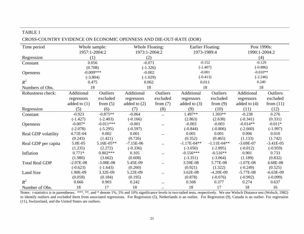
We report the associated regression results for the whole sample period (1957:1-2004:2)
New Zealand, Norway, Portugal, Spain, Sweden, Switzerland, the U.K., and the U.S.
7 Since we use quarterly data in the analysis, seasonality of price changes is expected. To properly account for theseasonal effect, we include seasonal dummies in equation (2) when estimating the DOR for each country.
6
in regression (1) of Table 1. The openness coefficient is negative (−0.009) and significant (t =
−3.804) at the 1% level. This result indicates that inflation shocks are less persistent and die out
faster in more open economies. Examining this results further, we see in relation to the sample
average of DOR of −0.22, a 1 standard deviation increase in economic openness (equivalent to 14
percentage points) decreases DOR (on average) by 0.58.8
Does this result hold for different time periods? Within the span of our sample period,
two widely mentioned international monetary regime shifts are 1973 and 1990. The year 1973
is associated with the breakdown of the Bretton Woods system, and the year 1990 is suggested
by the inflation targeting literature.9 To provide a preliminary indication regarding whether these
suggested breaks alter the behavior of monetary responses to inflation (in relation to openness), we
rerun regression (3) using these two pre-specified cutoff points.
We report the regression results for the subsample periods of "whole floating" (1973:1-
2004:2), "earlier floating" (1973:1-1989:4), and "post 1990s" (1990:1-2004:2) in regressions (2),
(3), and (4) of Table 1, respectively. The results show that the coefficient on openness for the post
1990s period is negative and significant but it is not significant for either the whole floating or ear-
lier floating periods. These results indicate that it is primary after the 1990s when inflation shocks
die out faster in more economically open countries. To ensure the robustness of these results, we
redo the analysis by adding various independent variables for rival arguments to equation (3), and
later by excluding outliers from sample countries.10 The associated regression results reported as
8 This result comes from the following calculation: (14.18×−0.009)/− 0.22 = 0.58, where the standard deviationof openness is 14.18 and the mean of DOR is −0.22.9 The inflation targeting literature suggests that there is a universal regime shift in the practice of monetary policysince the 1990s. The shift involves monetary authorities placing greater weight on reducing inflation instability (SeeBernanke, et. al. (1999) as a representative study).10 The literature has mentioned 4 factors, other than economic openness, which could affect monetary authorities’intentions/attitudes in fighting inflation. First, it is noted that a more severe supply shock tends to generate a largertrade-off between inflation and output volatilities. This larger trade-off in turn could induce policymakers to be lessaggressive in fighting inflation. We compute the variance of real output growth for each country to account for thesize of the supply shock. Second, we use the real GDP per capita to account for the potential influence of the status
7
regressions (5)-(12) in Table l show that our findings are robust.
With this cross-country evidence suggesting that more aggressive monetary policies are
being adopted in more open economies emerged in the 1990s, we raise the paper’s main concern:
if this emerging cross-country DOR-openness pattern in the 1990s is the result that the majority
of individual countries in our sample did have their monetary policies react most extensively to
economic openness as the 1990s approached. We set out the analysis in the rest of this paper to
answer this key question.
3. ECONOMIC OPENNESS AND DOR: EVIDENCE FROM INDIVIDUAL COUNTRY’S
TIME SERIES DATA
To assess the long-term relation between economic openness and the DOR in each individ-
ual country, we will use a rolling regression technique to generate the DOR and economic openness
time series for a country. The DOR time series for an individual country is obtained by running
regression (2) where we set the rolling regression window at 10 years (equivalent to 41quarters)
and move the window forward at a 1-quarter interval until we reach the last estimation window
of 1994:2-2004:2. For the economic openness time series, we generate the estimates based on an
economic theory that is widely used in a number of macroeconomics studies (see Romer (1993)).
3.1 Openness Data/Estimates from an Economic Theory
Macroeconomists assume that in an open economy, where international trade takes place,
the general domestic price takes the following form:
of economic development on the link between economic openness and inflation performance (see the argument inRomer (1993)). Third, we include the inflation level in our robustness regressions as it is primary a control variablein the majority of monetary policy regressions in the literature. Finally, some researchers note that there may be apotential impact from country size on the openness-inflation relation. We use total real GDP (as in Lane (1997)) andland size (as in Romer (1993)) to account for this effect.
8
pGt = wpft + (1− w)pdt , w ∈ [0, 1), (4)
where pGt is the log of the general domestic price level, pft is the log of the domestic price level
of foreign goods, pdt is the log of the domestic price level of domestic goods, and w represents the
share of domestic consumption of foreign goods and services. The coefficient of w is commonly
referred to as "economic openness" and it is aimed to capture the degree of the influence from
external factors (pft in this case) on the general domestic price level. For ease in imposition, a
large body of literature assigns values to w (openness) by simply calculating the ratio of imports
of goods and services to GDP.
To comply with economic theory, we will generate w (openness) using the relation ex-
pressed in equation (4). Since the data for pdt is unavailable for half of the countries in our sample,
following the literature, we write equation (4) into a more extensive form. First, assume that the
Law of One Price holds so that the domestic price of foreign goods is the same as the relative price
in the foreign market:
pft = et + p∗t , (5)
where et is the log of nominal exchange rate, defined in units of domestic currency per unit of
foreign currency, and p∗t is the foreign price of foreign goods.
Second, Macroeconomists believe that the price level in the domestic market is governed
by the quantity theory:
mt + vt = pdt + yt, (6)
where mt is the log of domestic money supply, vt is the log of velocity of money, and yt is the log
of real domestic output. Further, both Blanchard and Kiyotaki (1987) and Romer (1996) note that
it is appropriate to consider the velocity of money (vt) as the aggregate disturbance in countries
9
where there are no hyperinflations. Thus, a reduced form of the quantity theory can be expressed
as:
pdt = mt − yt. (7)
Now, substituting both equations (5) and (7) into (4) yields:
pGt = w(et + p∗t ) + (1− w)(mt − yt). (8)
Conceptually, the coefficient of w in equation (8) measures the effect of external factors - et and
p∗t , in comparison to that of internal factors - mt and yt, to affect the general domestic price level.
Alternatively, the size of w can also indicate how vulnerable the general domestic price level is
to external factors. In fact, researchers find this attribute intuitively appealing for their argument
regarding how a country’s monetary policy aggressiveness depends on how vulnerable the coun-
try’s price level is to external factors. We note that estimating the coefficient of w from equation
(8) and regarding it as openness data complies with our paper’s pursuit: examining whether his-
torical changes in monetary policy (aggressiveness) are the result of changes in the policymakers’
reactions to economic openness.
It is important to notice that most recently Lo and Wong (2006) validate the theoretical
predictions of equation (8) in a large sample of 63 countries. The robustness of their empirical
findings lend support for generating openness data using equation (8). In what follows, we assess
the relation among pGt , (et + p∗t ), and (mt − yt) to generate an economic openness time series for
each country in our sample:
pGt = γ + α(et + p∗t ) + β(mt − yt) (9)
As before, we use quarterly data from the IMF’s IFS. For each country, we use the CPI for
pGt ; money plus quasi-money for mt; GDP at a constant price for yt. We treat the largest trading
10
partner as the base foreign country for the domestic economy, and consequently we use the price of
the base foreign country’s currency and the base foreign country’s CPI for et and p∗t , respectively.11
The data are available at different lengths among sample countries. We use the maximum length
of data available for each country in the analysis. The longest data period we have for a country
is 1957:1-2004:2, while the shortest data period is 1987:4-2004:2. Table 2 lists the data length
available for each country.12
We use Hansen’s (1992) FMOLS (test statistics of Lc) to estimate the cointegrating relation
of equation (9).13 To be consistent with the length of the DOR series, when generating the openness
series of α, we also set the estimation window at 41 quarters and we move it forward for 1-quarter
each iteration. Hansen (1992) cautions that rejection of the null hypothesis only provides evidence
that a "standard" cointegration model does not hold ("standard" in the sense that a structural break
is not included in cointegrating regressions). In a few cases where the Lc test statistics reject
the null hypothesis, we perform Gregory and Hansen’s (1996) residual-based test (G&H test) to
identify where the level regime shift (model 2 of the G&H test) occurs. We then estimate the
cointegration coefficients of α and β by modifying equation (9) to include a level shift dummy, as
identified by the G&H tests.
3.2 Initial Results with Pre-specifying Cutoff Points
To examine the potential historical changes in monetary policy aggressiveness to economic
openness in individual countries, we initially regress each country’s DOR series on its own eco-
11 The foreign country with the largest share of trade (imports plus exports) within a domestic country is regarded asthe largest trading partner (for the domestic country). The data source is CIA-The World Factbook. Detailed dataare available on request.12 For countries participating in the European Monetary Union (EMU), their sample period ends earlier than that ofother countries in our sample. This situation is because their exchange rate data ends at 1998:4.13 A precondition for the existence of a cointegrating relation in equation (9) is that all three variables of pGt , et+ p∗t ,and mt − y are nonstationary (i.e. I(1)). Using the unit root test of DF-GLS proposed by Elliott et. al. (1996), wefind the data for the full sample period from all 18 sample countries meets this precondition. Unit root results are notreported here but are available on request.
11
nomic openness series across different sample periods via pre-specified cutoff points:
DORi,t = hi,t + ki,tOPENBi,t + υi,t, (10)
where DORi,t is country i’s die-out-rate time series at period t (generated via equation (2));
OPENBi,t is country i’s openness time series at period t (generated via equation (9)); and υi,t
is a stochastic term. Besides two earlier used cutoff points of 1973:1 and 1990:1, we now include
1985:4 to further divide the sample period. This added cutoff point is a data management consider-
ation: EMU countries in our sample do not have their post 1990s period available for the analysis.
Since EMU countries’ exchange rate data ends at 1998:4, it is not feasible to generate their 1st
openness data point for the post 1990s period (requiring raw data of 1990:1-2000:1). This situa-
tion constrains our ability to check whether monetary policies react more extensively to economic
openness as the 1990s approached. We therefore use the Plaza Agreement (reached in September
1985) as an additional cutoff point. The Plaza Agreement was made by the G-5 countries in an
effort to depress the value of $US by means of coordinated interventions in the foreign exchange
markets. This exchange rate agreement could potentially change monetary policy behavior as it
forces policymakers among countries to be more accommodative to each other’s policy initiatives.
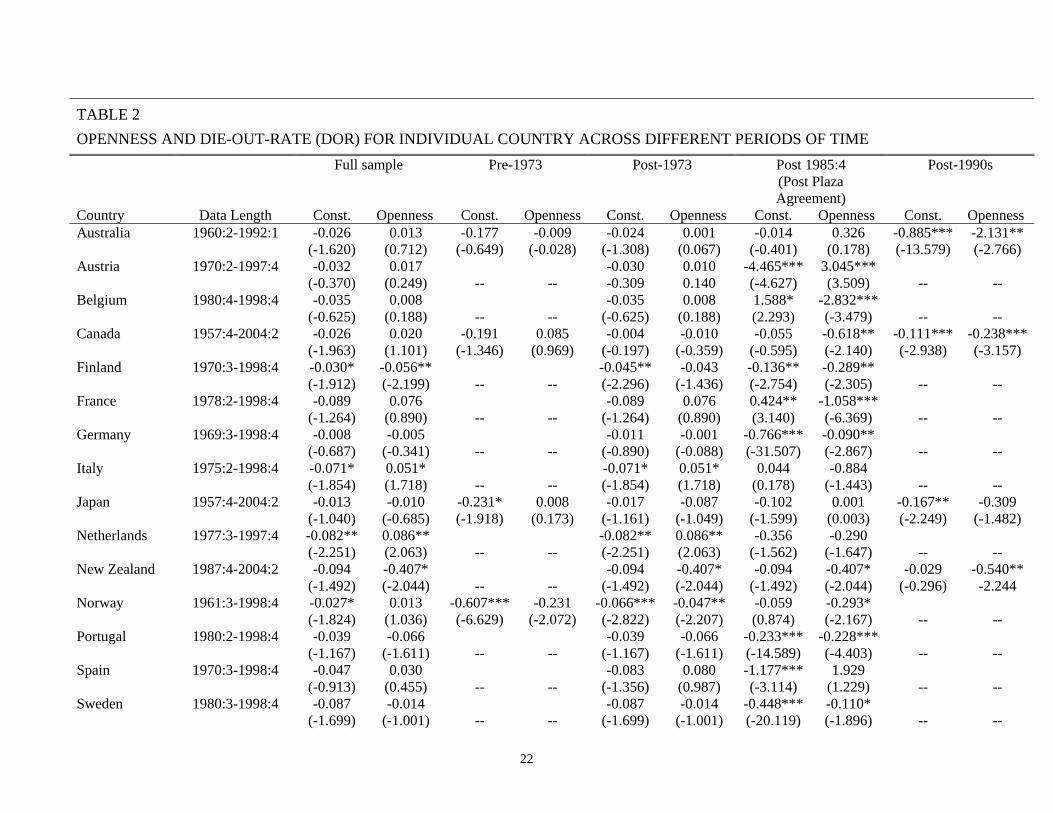
Table 2 summarizes estimation results for equation (10) across the full sample period, and
4 subsample periods of Pre-1973, Post-1973, the Post-1985:4 (the Post Plaza Agreement), and
the Post-1990s. For the full sample period’s results, we find no evidence of a negative DOR-
openness relation except for two countries (Finland and New Zealand). We next compare results
from different subsample periods. Since we lack raw data for most countries in the Pre-1973
period, we focus attention on results from the Post-1973 period. The results for the Post-1973
period are similar to those for the full sample period: very little empirical support for the negative
12
DOR-openness relation. Alternatively, for either the full sample period or the Post-1973 period, we
do not find a pattern that more aggressive monetary responses were used as an economy becomes
more open. Yet, such patterns start to emerge when the time period approaches the 1990s. Under
the Post-1985:4 (the Post Plaza Agreement) period, results from 9 countries (out of 18) give a
significant negative DOR-openness relation. These countries include Belgium, Canada, Finland,
France, Germany, New Zealand, Norway, Portugal, and Sweden. This negative relation emerges
for 2 additional countries, Australia and the U.S., when moving into the Post-1990s period.
Overall, these initial results with pre-specified cutoff points indicate that about 61% (=
11/18) of the sample countries seem to have shifted, around 1985-1990, in their monetary policy
making. That is, policymakers in more recent years seem to conduct monetary policy in reaction
to changes in the degree of economic openness. To validate this emerging shift in monetary policy
making, we next apply Bai and Perron’s (1998, 2003, henceforth BP) methodology, designed to
formally test and date multiple structural breaks.
3.3 Results with Structural Break Points Being Identified by BP Methodology
Using procedures developed by BP, our investigation will be at two levels.14 First, we
examine whether individual countries experience breaks (particularly in the neighborhood of Post-
1985 or Post-1990s period) in monetary policy making. If there are indeed monetary policy shifts
dated in recent years, we then proceed with our second examination – whether these breaks are
associated with changes in policy responses to economic openness.
We perform our first test by using BP’s procedures to sequentially search for structural
breaks (if any) in equation (2) for all 18 countries.15 We consider the possibility that equation
14 The BP procedures, which we use to generate this paper’s results, are available at Pierre Perron’s website:http://people.bu.edu/perron/code.html.15 Since BP procedures allow autocorrelation and heteroskedasticity in the regression model residuals, we do notinclude any lags of the dependent variables as the explanatory variables in equation (2) to remove potential serial
13
(2) is a "pure" structural change model ("pure" in the sense that both the constant term (c) and
the DOR parameter (d) are allowed to change). BP (2003) caution that there are instances where
the sequential procedure can be improved. They refer to instances where there exists multiple
structural breaks. In such cases, it is difficult for the sequential test statistics (supFT (l + 1|l))
to reject the null hypothesis of no break versus one break but not difficult to reject the null of
no breaks versus a higher number of breaks. To deal with this problem, BP’s recommendation
is to examine double maximum test statistics (WD max or UD max) and determine if at least
one break exists. If the answer is affirmative, then we proceed with a sequential examination (but
ignore supFT (1|0)) to determine the maximum number of breaks in the regression model. We
follow this recommendation in all relevant test applications.
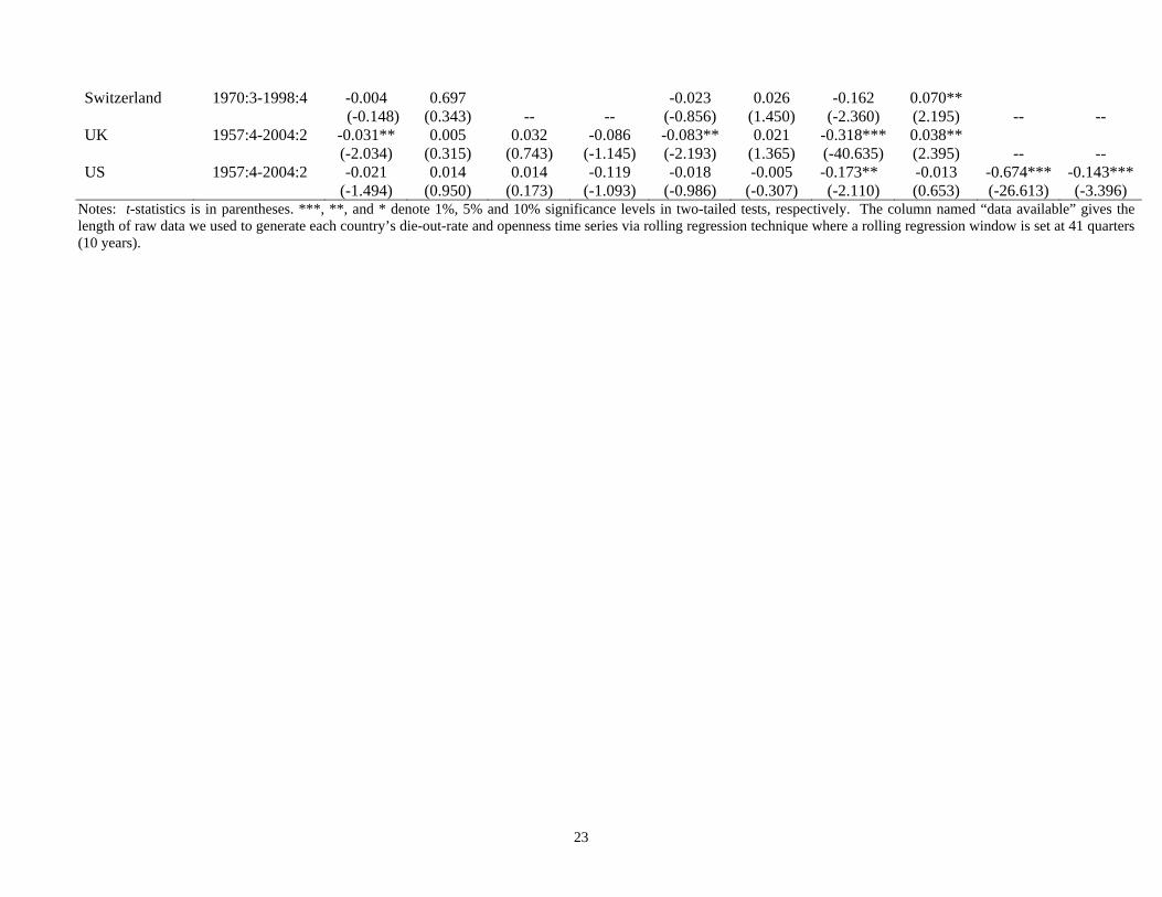
Panel A of Table 3 reports BP test statistics (of WD max, and supFT (l + 1|l)) and dates
for the structural breaks on the regression model of (2) for each of the 18 counties. The uniform
rejection by the test statistics of WD max for all 18 countries indicates that there is at least one
regime shift in each country for the regression of (2). The estimation results for break points (re-
ported in the last column of Panel A in Table 3) show that many countries did have a monetary
policy regime shift in the neighborhood of the 1985 to 1990s period. There are only 3 exceptions:
Germany, Italy and the U.K. appear to have their most recent monetary policy (toward inflation)
change prior to 1985 (1982:4 for both Germany and Italy, and 1981:2 for the U.K.). Using these
identified break points as cutoff points for the whole sample period, we redo the estimation on re-
gression (2) for each country under different sample periods. Panel B of Table 3 reports associated
regression results. Our focus is on the changes in the size of coefficient "d" (i.e., DOR).
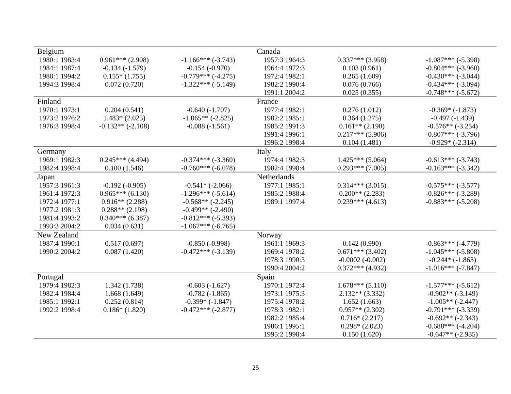
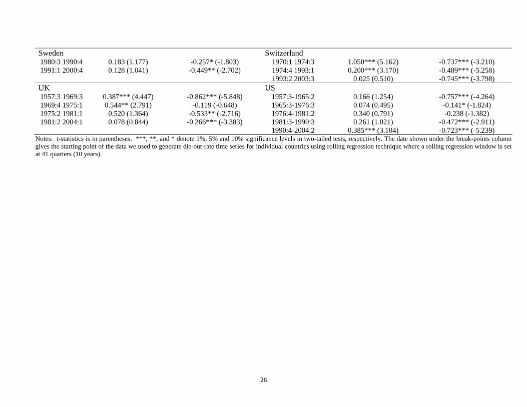
One important trend we observe is that 13 (out of 18) countries have their inflation shocks
die out faster in the last regime sample period rather than the previous one. Using the case of thecorrelation in the residuals.
14
U.S. for illustration, the DOR from the last regime period of 1990:4-2004:2 is -0.723. This is larger
in absolute terms than -0.472, the DOR from the previous regime period of 1981:3-1990:3. Coun-
tries with this pattern include Australia, Belgium, Canada, France, Germany, Japan, Netherlands,
New Zealand, Norway, Portugal, Sweden, Switzerland, and the U.S. Further, among these 13 coun-
tries, 8 countries’ DOR from the last regime period is the largest (in absolute value) in comparison
to that from any other regime period.16 We interpret these results as evidence that there are histori-
cal regime shifts in monetary policy making among all sample countries. In addition, it is evident
that the monetary regime shift in recent years is more of a universal similarity: policymakers in
many developed countries have dealt with inflation shocks much more aggressively.
With this evidence, we proceed to use BP procedures to perform our second examination –
the main concern of this paper: Can the observed historical changes in the size of the DOR in in-
dividual countries be linked to shifts in the monetary authorities’ reaction to economics openness?
For each of the 18 countries, we now sequentially search for structural breaks in equation (10),
which aims to capture the DOR-openness relation. While we consider a pure structural change
model in this examination, our focus is more toward the changes in the openness parameter (k) in
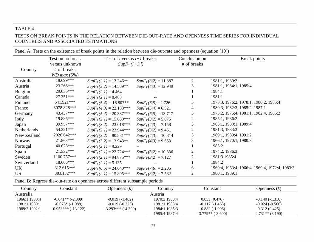
equation (10). Panel A of Table 4 gives results on test statistics used to determine the numbers of
structural breaks for each country, and associated dates for the breaks.
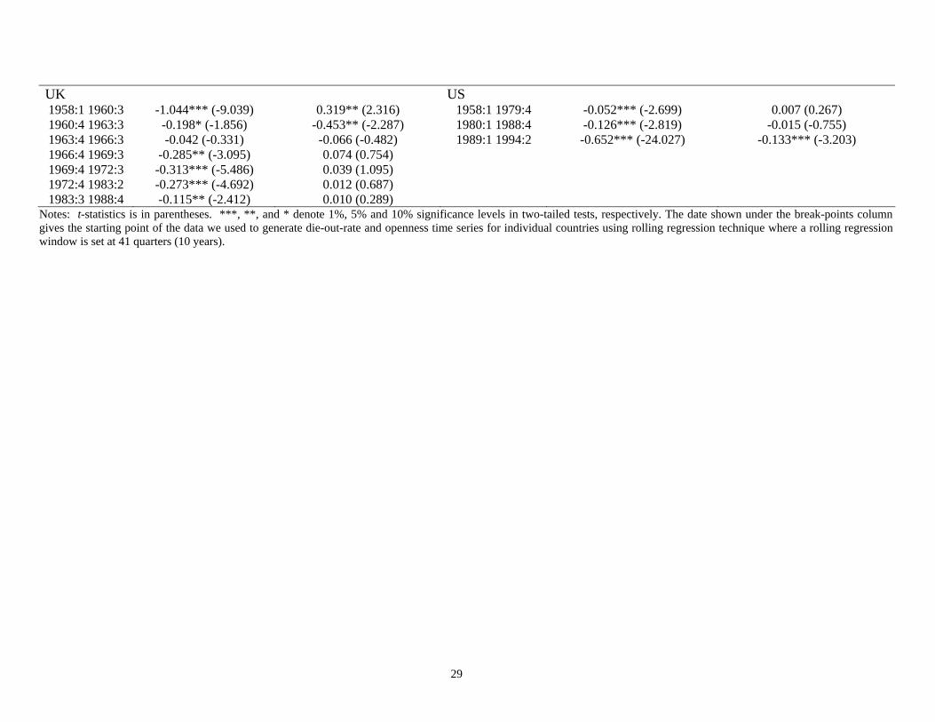
The results show that all 18 countries have at least one structural break in the DOR-
openness relation. More importantly, the majority of countries did have their most recent break
dated in the neighborhood of 1985-1990, except for Canada, Norway, and the U.K. For these three
countries, the most recent break is dated prior to 1985 (1981:1, 1980:3 and 1983:3 for Canada,
Norway, and the U.K, respectively).
16 They are Belgium, France, Germany, Netherlands, New Zealand, Portugal, Sweden, and Switzerland.
15
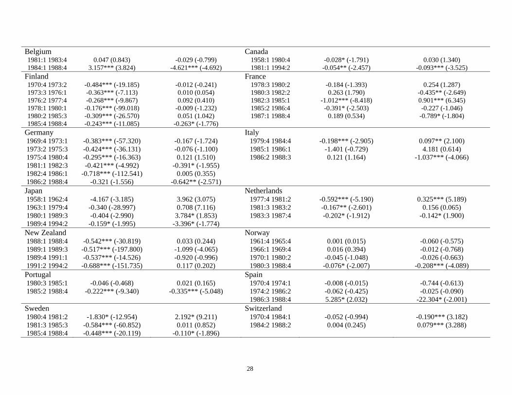
Using these break points, we cut each country’s entire sample period into various regime
periods and re-run equation (10). We report associated regression results in Panel B of Table 4. A
trend we find is that there are 14 out of 18 country’s openness parameter(s) from the "last" regime
period now become significantly negative. These countries are Australia, Belgium, Canada, Fin-
land, France, Germany, Italy, Japan, Netherlands, Norway, Portugal, Spain, Sweden, and the U.S.
The openness parameter in these 14 countries from the prior regime period is either statistically in-
distinguishable from zero or showing a positive sign. We note that this universal shift is particularly
striking in that the emerging negative DOR-openness relation has no precedent (prior to the last
regime period) in 12 out of 14 countries.17 These results provide evidence that monetary author-
ities in the majority of developed countries did start to adjust their inflation stabilization policies
in reaction to their economic openness in recent years. The pattern of such a reaction is that when
the economy becomes more (less) open over time, the monetary authorities tend to act more (less)
aggressively to counteract the inflation shocks.
4. CONCLUSIONS
In this paper, we provide empirical evidence, in a sample of 18 developed countries, docu-
menting that economic openness is a compelling factor in the international differences in monetary
policy aggressiveness to inflation shocks.
To measure the aggressiveness of monetary policy in counteracting inflation shocks, we use
the estimate of DOR (die-out-rate of inflation shocks). If policymakers act more aggressively in
response to inflation shocks, these shocks would be less persistent and the estimate of DOR would
be observed to be negative and larger in absolute value.
17 They are Australia, Belgium, Canada, Finland, Italy, Japan, Netherlands, Norway, Portugal, Spain, Sweden, andthe U.S.
16
The central argument of this paper is motivated by a rationale from the economic openness-
inflation literature. This literature examines how economic openness influences international dif-
ferences in the responsiveness of monetary policy (to inflation) because economic openness raises
the potential cost of high inflation. Specifically, this literature suggests a negative economic
openness-inflation relation across countries. Following this rationale, we argue a policymaker
within his own country would also adjust the aggressiveness of monetary policy according to
changes in the degree of economic openness.
Our empirical results across countries show a negative openness-DOR relation. This nega-
tive relation indicates that more an aggressive monetary policy is adopted in more open economies.
More importantly, the results show that it is primary after the 1990s when inflation shocks die out
faster in more open countries. Using this cross-country evidence as the basis for the paper’s cen-
tral argument, that economic openness can account for monetary policy attitude changes within
a country, we examine data at the individual-country level. The initial result with pre-specified
cutoff points find no evidence of a negative openness-DOR relation in any sample period prior to
the 1990s. Yet, the negative relation starts to emerge when the time period approaches the 1990s.
These findings suggest that countries in our sample seem to have shifted around 1985-1990 in their
monetary policy making in reaction to changes in their degree of economic openness. Applying
BP methodology (to formally test and date structural breaks in the data) validates this emerging
shift in monetary policy making in the 1990s. We find that the majority of countries in the sample
have their DOR estimates shift in a more negative direction as the 1990s ensued. We interpret this
result as evidence that policymakers in many developed countries have dealt with inflation shocks
much more aggressively after the 1990s. Further, we find that the majority of countries in the
sample also have their openness-DOR relation shift to a significant negative sign when entering
17
the 1990s.
Taken all this evidence together, this paper has documented that changes in the DOR (an al-
ternative estimate of inflation persistence) in recent years is a stylized international phenomena that
has a coherent explanation. The recent universal decrease in the persistence of inflation shocks is
a reflection of monetary authorities in many (developed) countries adjusting the aggressiveness of
monetary policy responses according to changes in the degree of openness within their economies.
This universal change in monetary policy making at the individual country level serves as a basis
for the documented cross-country pattern that more aggressive monetary policies were adopted in
more open economies (primarily) in the 1990s.
18
19
References
Alogoskoufis, George S. 1992. The Monetary accommodation, exchange rate regimes and inflation
persistence. Economic Journal 102:461—480.
Alogoskoufis, George S., and Ron Smith. 1991. The Phillips curves, the persistence of inflation, and
the Lucas critique: Evidence from exchange-rate regimes. American Economic Review 81:1254—
1275.
Bai, Jushan, and Pierre Perron. 1998. Estimating and testing linear models with multiple structural
changes. Econometrica 66: 47—68.
Bai, Jushan, and Pierre Perron. 2003. Computation and analysis of multiple structural change
models. Journal of Applied Econometrics 18: 1—22.
Bernanke, Ben S., Thomas Laubach, Frederic S. Mishkin, and Adam Posen. 1999. Inflation
Targeting. New Jersey: Princeton University Press.
Blanchard, O. and N. Kiyotaki. 1987. Monopolistic competition and the effects of aggregate
demand. American Economic Review 77: 647—666.
Bleaney, Michael. 2001. Exchange rate regimes and inflation persistence. IMF Staff papers 47:
387—402.
Burdekin, C. K. Richard and Pierre L. Siklos. 1999. Exchange rate regimes and shifts in inflation
persistence: Does nothing else matter? Journal of Money, Credit and Banking 31:235—247.
Clarida, Richard, Jordi Gali, and Mark Gertler. 2001. Optimal monetary policy in open versus
closed economies: An integrated approach. AEA Papers and Proceedings 91:248—252.
Clarida, Richard, Jordi Gali, and Mark Gertler. 2002. A simple framework for international
monetary policy analysis. Journal of Monetary Economics 49:879—904.
Dornbusch, Rudiger. 1982. PPP exchange rate rules and macroeconomic stability. Journal of
Political Economy 90:1033—1067.
Elliott, Graham, Thomas J. Rothenberg, and James H. Stock. 1996. Efficient tests for an
autoregressive unit root. Econometrica 64:813—836.
Frankel, Jeffrey A., and Andrew K. Rose. 1996. A panel project on purchasing power parity: Mean
reversion within and between countries. Journal of International Economics 40:209—24.
Granato Jim, Melody Lo, and Sunny, M. C. Wong. 2006. Testing monetary policy intentions in
open economies. Southern Economic Journal 72:730—746.
20
Gregory, A., and B. Hansen. 1996. Residual-based tests for cointegration in models with regime
shifts. Journal of Econometric 70: 99—126.
Hansen, B. 1992. Tests for parameter instability in regressions with I(1) processes. Journal of
Business and Economic Statistics 10: 321—335.
Lane, Phillip R. 1997. Inflation in open economies. Journal of International Economics 42:327—
347.
Lo, Melody, and Sunny, M. C. Wong. 2006. What explains the deviations of purchasing power
parity across countries? International evidence from macro data. Economics Letters 91: 229—235.
Lucas, Robert E., Jr. 1976. Econometric policy evaluation: A critique. In the Phillips Curve and
Labor Market, edited by Karl Brunner and Allan H. Meltzer. Amsterdam: North-Holland, pp.
19—46.
Obstfeld, Maurice. 1995. International currency experiences: New lessons and lessons relearned.
Brookings Papers on Economic Activity: 1, Brookings Institution, pp. 119-220.
Perron, Pierre, and Timothy J. Vogelsang. Nonstationarity and level shifts with an application to
purchasing power parity. Journal of Business and Economic Statistics 10: 301-320.
Romer, David H. 1993. Openness and inflation: theory and evidence. Quarterly Journal of
Economics 108:869—903.
Romer, David H. 1996. Advanced Macroeconomics. New York: McGraw-Hill.
Siklos, Pierre L. 1999. Inflation-target design: Changing inflation performance and persistence in
industrial countries. Review: Federal Reserve Bank of St. Louis March/April:47—58.
Taylor, John B. 1993. Discretion versus policy rules in practice. Carnegie Rochester Conference
Series on Public Policy 39:195—214.
Temple, Jonathan R. W. 2002. Openness, inflation, and the Phillips curve: a puzzle. Journal of
Money, Credit and Banking 34:450—468.
Welsch, Roy E. 1982. Influence functions and regression diagnostics. In Modern Data Analysis,
edited by R. L. Launer and A.F. Siegel. New York: Academic Press, pp. 149—169.
21
TABLE 1
CROSS-COUNTRY EVIDENCE ON ECONOMIC OPENNESS AND DIE-OUT-RATE (DOR)
Time period Whole sample: Whole Floating: Earlier Floating: Post 1990s: 1957:1-2004:2 1973:1-2004:2 1973-1989:4 1990:1-2004:2 Regression (1) (2) (4) Constant 0.056
(0.708) -0.071
(-1.326) -0.152
(-1.407) -0.129
(-0.886) Openness -0.009***
(-3.804) -0.002
(-1.029) -0.001
(-0.413) -0.010** (-2.246)
R2 0.475 0.062 0.011 0.240 Numbers of Obs. 18 18 18 18 Robustness check: Additional
regressors added to (1)
Outliers excluded from (5)
Additional regressors
added to (2)
Outliers excluded from (7)
Additional regressors
added to (3)
Outliers excluded from (9)
Additional regressors
added to (4)
Outliers excluded from (11)
Regression (5) (6) (7) (8) (9) (10) (11) (12) Constant -0.923
(-1.427) -0.875** (-2.403)
-0.064 (-0.166)
--
1.497** (2.863)
1.393** (2.638)
-0.238 (-0.341)
0.276 (0.331)
Openness -0.007* (-2.078)
-0.011*** (-5.295)
-0.001 (-0.597)
--
-0.003 (-0.844)
-0.003 (-0.806)
-0.014** (-2.660)
-0.011* (-1.997)
Real GDP volatility 4.71E-04 (0.243)
0.002 (1.421)
0.001 (0.726)
--
0.001 (0.352)
0.001 (0.465)
0.006 (1.133)
0.010 (1.742)
Real GDP per capita 5.0E-05 (1.235)
5.16E-05** (2.272)
-7.15E-06 (-0.336)
--
-1.17E-04** (-3.050)
-1.11E-04** (-2.895)
-3.69E-07 (-0.012)
-3.41E-05 (-0.959)
Inflation 0.771* (1.980)
0.802*** (3.662)
0.105 (0.608)
--
-0.556*** (-3.351)
-0.516** (-3.064)
0.901 (1.189)
0.733 (0.832)
Total Real GDP -2.07E-08 (-0.623)
-3.08E-08 (-1.643)
5.45E-09 (0.260)
--
3.59E-08 (0.921)
5.77E-08 (1.322)
-1.07E-08 (-0.249)
4.68E-08 (0.525)
Land Size 1.90E-09 (0.059)
3.32E-09 (0.184)
5.22E-09 (0.195)
--
3.62E-08 (0.878)
-4.20E-09 (-0.076)
-5.77E-08 (-0.992)
-6.63E-09 (-0.099)
R2 0.666 0.903 0.242 -- 0.568 0.377 0.274 0.637 Number of Obs. 18 17 18 -- 18 17 18 16
Notes: t-statistics is in parentheses. ***, **, and * denote 1%, 5% and 10% significance levels in two-tailed tests, respectively. We use Welsch Distance test (Welsch, 1982) to identify outliers and excluded them from associated regressions. For Regression (5), Netherlands is an outlier. For Regression (9), Canada is an outlier. For regression (11), Switzerland, and the United States are outliers.
22
TABLE 2
OPENNESS AND DIE-OUT-RATE (DOR) FOR INDIVIDUAL COUNTRY ACROSS DIFFERENT PERIODS OF TIME
Full sample Pre-1973 Post-1973 Post 1985:4 (Post Plaza Agreement)
Post-1990s
Country Data Length Const. Openness Const. Openness Const. Openness Const. Openness Const. Openness Australia 1960:2-1992:1
-0.026
(-1.620) 0.013
(0.712) -0.177
(-0.649) -0.009
(-0.028) -0.024
(-1.308) 0.001
(0.067) -0.014
(-0.401) 0.326
(0.178) -0.885*** (-13.579)
-2.131** (-2.766)
Austria 1970:2-1997:4
-0.032 (-0.370)
0.017 (0.249)
--
--
-0.030 -0.309
0.010 0.140
-4.465*** (-4.627)
3.045*** (3.509)
--
--
Belgium 1980:4-1998:4
-0.035 (-0.625)
0.008 (0.188)
--
--
-0.035 (-0.625)
0.008 (0.188)
1.588* (2.293)
-2.832*** (-3.479)
--
--
Canada 1957:4-2004:2
-0.026 (-1.963)
0.020 (1.101)
-0.191 (-1.346)
0.085 (0.969)
-0.004 (-0.197)
-0.010 (-0.359)
-0.055 (-0.595)
-0.618** (-2.140)
-0.111*** (-2.938)
-0.238*** (-3.157)
Finland 1970:3-1998:4
-0.030* (-1.912)
-0.056** (-2.199)
--
--
-0.045** (-2.296)
-0.043 (-1.436)
-0.136** (-2.754)
-0.289** (-2.305)
--
--
France
1978:2-1998:4
-0.089 (-1.264)
0.076 (0.890)
--
--
-0.089 (-1.264)
0.076 (0.890)
0.424** (3.140)
-1.058*** (-6.369)
--
--
Germany
1969:3-1998:4
-0.008 (-0.687)
-0.005 (-0.341)
--
--
-0.011 (-0.890)
-0.001 (-0.088)
-0.766*** (-31.507)
-0.090** (-2.867)
--
--
Italy
1975:2-1998:4
-0.071* (-1.854)
0.051* (1.718)
--
--
-0.071* (-1.854)
0.051* (1.718)
0.044 (0.178)
-0.884 (-1.443)
--
--
Japan
1957:4-2004:2
-0.013 (-1.040)
-0.010 (-0.685)
-0.231* (-1.918)
0.008 (0.173)
-0.017 (-1.161)
-0.087 (-1.049)
-0.102 (-1.599)
0.001 (0.003)
-0.167** (-2.249)
-0.309 (-1.482)
Netherlands
1977:3-1997:4
-0.082** (-2.251)
0.086** (2.063)
--
--
-0.082** (-2.251)
0.086** (2.063)
-0.356 (-1.562)
-0.290 (-1.647)
--
--
New Zealand
1987:4-2004:2
-0.094 (-1.492)
-0.407* (-2.044)
--
--
-0.094 (-1.492)
-0.407* (-2.044)
-0.094 (-1.492)
-0.407* (-2.044)
-0.029 (-0.296)
-0.540** -2.244
Norway
1961:3-1998:4
-0.027* (-1.824)
0.013 (1.036)
-0.607*** (-6.629)
-0.231 (-2.072)
-0.066*** (-2.822)
-0.047** (-2.207)
-0.059 (0.874)
-0.293* (-2.167)
--
--
Portugal
1980:2-1998:4
-0.039 (-1.167)
-0.066 (-1.611)
--
--
-0.039 (-1.167)
-0.066 (-1.611)
-0.233*** (-14.589)
-0.228*** (-4.403)
--
--
Spain
1970:3-1998:4
-0.047 (-0.913)
0.030 (0.455)
--
--
-0.083 (-1.356)
0.080 (0.987)
-1.177*** (-3.114)
1.929 (1.229)
--
--
Sweden
1980:3-1998:4
-0.087 (-1.699)
-0.014 (-1.001)
--
--
-0.087 (-1.699)
-0.014 (-1.001)
-0.448*** (-20.119)
-0.110* (-1.896)
--
--
23
Switzerland
1970:3-1998:4
-0.004 (-0.148)
0.697 (0.343)
--
--
-0.023 (-0.856)
0.026 (1.450)
-0.162 (-2.360)
0.070** (2.195)
--
--
UK
1957:4-2004:2
-0.031** (-2.034)
0.005 (0.315)
0.032 (0.743)
-0.086 (-1.145)
-0.083** (-2.193)
0.021 (1.365)
-0.318*** (-40.635)
0.038** (2.395)
-- --
US
1957:4-2004:2
-0.021 (-1.494)
0.014 (0.950)
0.014 (0.173)
-0.119 (-1.093)
-0.018 (-0.986)
-0.005 (-0.307)
-0.173** (-2.110)
-0.013 (0.653)
-0.674*** (-26.613)
-0.143*** (-3.396)
Notes: t-statistics is in parentheses. ***, **, and * denote 1%, 5% and 10% significance levels in two-tailed tests, respectively. The column named “data available” gives the length of raw data we used to generate each country’s die-out-rate and openness time series via rolling regression technique where a rolling regression window is set at 41 quarters (10 years).
24
TABLE 3
TESTS ON BREAK POINTS IN THE DIE-OUT-RATE TIME SERIES FOR INDIVIDUAL COUNTRIES AND ASSOCIATED ESTIMATIONS
Panel A: Tests on the existence of break points for the die-out-rate time series (equation (2))
Country
Test on no break versus unknown
# of breaks: WD max (5%)
Test of l versus l+1 breaks: SupFT (l+1|l)
Conclusion on
# of breaks
Break points
Australia 27.624*** SupFT (3|2) = 33.932*** SupFT (4|3) = 8.644 3 1972:4, 1977:1, 1990:4 Austria 41.162*** SupFT (2|1) = 5.323 -- 1 1984:1 Belgium 33.564*** SupFT (3|2) = 12.728* SupFT (4|3) = 6.889 3 1984:1, 1988:1, 1994:3 Canada 48.854*** SupFT (4|3) = 16.414** SupFT (5|4) = 4.095 4 1964:4, 1972:4, 1982:2, 1991:1 Finland 32.945*** SupFT (2|1) = 17.881*** SupFT (3|2) = 10.191 2 1973:2, 1976:3 France 26.980*** SupFT (4|3) = 15.043** SupFT (5|4) = 4.878 4 1982:2, 1985:2, 1991:4, 1996:2 Germany 18.913*** SupFT (2|1) = 4.473 -- 1 1982:4 Italy 15.889** SupFT (2|1) = 10.091 -- 1 1982:4 Japan 29.580*** SupFT (5|4) = 21.095*** SupFT (6|5) = 9.984 5 1961:4, 1972:4, 1977:2, 1981:4, 1993:3 Netherlands 28.228*** SupFT (2|1) = 12.973** SupFT (3|2) = 10.840 2 1985:2, 1989:1 New Zealand 14.598** SupFT (2|1) = 8.603 -- 1 1990:2 Norway 46.999*** SupFT (3|2) = 15.048** SupFT (4|3) = 6.317 3 1969:4, 1978:3, 1990:4 Portugal 28.507*** SupFT (3|2) = 31.695*** SupFT (4|3) = 11.456 3 1982:4, 1985:1, 1992:2 Spain 32.813*** SupFT (6|5) = 29.163*** SupFT (7|6) = 11.428 6 1973:1, 1975:4, 1978:3, 1982:2, 1986:1, 1995:2 Sweden 26.047*** SupFT (2|1) = 4.484 -- 1 1991:1 Switzerland 23.605*** SupFT (2|1) = 29.283*** SupFT (3|2) = 11.769 2 1974:4, 1993:2 UK 17.201** SupFT (3|2) = 14.945** SupFT (4|3) = 11.063 3 1969:4, 1975:2, 1981:2 US 32.829*** SupFT (4|3) = 17.691** SupFT (5|4) = 6.462 4 1965:3, 1976:4, 1981:3, 1990:4
Panel B: Estimates of die-out-rate across different subsample periods
Country Constant Die-out-rate (d) Country Constant Die-out-rate (d) Australia Austria 1957:3-1972:3 0.043 (0.624) -0.019 (-0.247) 1969:3-1983:4 0.162* (1.803) -0.475*** (-4.123) 1972:4-1976:4 1.664*** (4.845) -0.973*** (-3.871) 1984:1-1997:4 -0.095 (-0.853) -0.460* (-1.896) 1977:1-1990:3 0.310** (2.357) -0.104 (-0.758) 1990:4-2000:1 0.139 (1.321) -0.770*** (-4.607)
25
Belgium Canada 1980:1 1983:4 0.961*** (2.908) -1.166*** (-3.743) 1957:3 1964:3 0.337*** (3.958) -1.087*** (-5.398) 1984:1 1987:4 -0.134 (-1.579) -0.154 (-0.970) 1964:4 1972:3 0.103 (0.961) -0.804*** (-3.960) 1988:1 1994:2 0.155* (1.755) -0.779*** (-4.275) 1972:4 1982:1 0.265 (1.609) -0.430*** (-3.044) 1994:3 1998:4 0.072 (0.720) -1.322*** (-5.149) 1982:2 1990:4 0.076 (0.766) -0.434*** (-3.094)
1991:1 2004:2 0.025 (0.355) -0.748*** (-5.672) Finland France 1970:1 1973:1 0.204 (0.541) -0.640 (-1.707) 1977:4 1982:1 0.276 (1.012) -0.369* (-1.873) 1973:2 1976:2 1.483* (2.025) -1.065** (-2.825) 1982:2 1985:1 0.364 (1.275) -0.497 (-1.439) 1976:3 1998:4 -0.132** (-2.108) -0.088 (-1.561) 1985:2 1991:3 0.161** (2.190) -0.576** (-3.254)
1991:4 1996:1 0.217*** (5.906) -0.807*** (-3.796) 1996:2 1998:4 0.104 (1.481) -0.929* (-2.314)
Germany Italy 1969:1 1982:3 0.245*** (4.494) -0.374*** (-3.360) 1974:4 1982:3 1.425*** (5.064) -0.613*** (-3.743) 1982:4 1998:4 0.100 (1.546) -0.760*** (-6.078) 1982:4 1998:4 0.293*** (7.005) -0.163*** (-3.342) Japan Netherlands 1957:3 1961:3 -0.192 (-0.905) -0.541* (-2.066) 1977:1 1985:1 0.314*** (3.015) -0.575*** (-3.577) 1961:4 1972:3 0.965*** (6.130) -1.296*** (-5.614) 1985:2 1988:4 0.200** (2.283) -0.826*** (-3.289) 1972:4 1977:1 0.916** (2.288) -0.568** (-2.245) 1989:1 1997:4 0.239*** (4.613) -0.883*** (-5.208) 1977:2 1981:3 0.288** (2.198) -0.499** (-2.490) 1981:4 1993:2 0.340*** (6.387) -0.812*** (-5.393) 1993:3 2004:2 0.034 (0.631) -1.067*** (-6.765) New Zealand Norway 1987:4 1990:1 0.517 (0.697) -0.850 (-0.998) 1961:1 1969:3 0.142 (0.990) -0.863*** (-4.779) 1990:2 2004:2 0.087 (1.420) -0.472*** (-3.139) 1969:4 1978:2 0.671*** (3.402) -1.045*** (-5.808)
1978:3 1990:3 -0.0002 (-0.002) -0.244* (-1.863) 1990:4 2004:2 0.372*** (4.932) -1.016*** (-7.847)
Portugal Spain 1979:4 1982:3 1.342 (1.738) -0.603 (-1.627) 1970:1 1972:4 1.678*** (5.110) -1.577*** (-5.612) 1982:4 1984:4 1.668 (1.649) -0.782 (-1.865) 1973:1 1975:3 2.132** (3.332) -0.902** (-3.149) 1985:1 1992:1 0.252 (0.814) -0.399* (-1.847) 1975:4 1978:2 1.652 (1.663) -1.005** (-2.447) 1992:2 1998:4 0.186* (1.820) -0.472*** (-2.877) 1978:3 1982:1 0.957** (2.302) -0.791*** (-3.339)
1982:2 1985:4 0.716* (2.217) -0.692** (-2.343) 1986:1 1995:1 0.298* (2.023) -0.688*** (-4.204) 1995:2 1998:4 0.150 (1.620) -0.647** (-2.935)
26
Sweden Switzerland 1980:3 1990:4 0.183 (1.177) -0.257* (-1.803) 1970:1 1974:3 1.050*** (5.162) -0.737*** (-3.210) 1991:1 2000:4 0.128 (1.041) -0.449** (-2.702) 1974:4 1993:1 0.200*** (3.170) -0.489*** (-5.258)
1993:2 2003:3 0.025 (0.510) -0.745*** (-3.798) UK US 1957:3 1969:3 0.387*** (4.447) -0.862*** (-5.848) 1957:3-1965:2 0.166 (1.254) -0.757*** (-4.264) 1969:4 1975:1 0.544** (2.791) -0.119 (-0.648) 1965:3-1976:3 0.074 (0.495) -0.141* (-1.824) 1975:2 1981:1 0.520 (1.364) -0.533** (-2.716) 1976:4-1981:2 0.340 (0.791) -0.238 (-1.382) 1981:2 2004:1 0.078 (0.844) -0.266*** (-3.383) 1981:3-1990:3 0.261 (1.021) -0.472*** (-2.911)
1990:4-2004:2 0.385*** (3.104) -0.723*** (-5.239) Notes: t-statistics is in parentheses. ***, **, and * denote 1%, 5% and 10% significance levels in two-tailed tests, respectively. The date shown under the break-points column gives the starting point of the data we used to generate die-out-rate time series for individual countries using rolling regression technique where a rolling regression window is set at 41 quarters (10 years).
27
TABLE 4
TESTS ON BREAK POINTS IN THE RELATION BETWEEN DIE-OUT-RATE AND OPENNESS TIME SERIES FOR INDIVIDUAL COUNTRIES AND ASSOCIATED ESTIMATIONS
Panel A: Tests on the existence of break points in the relation between die-out-rate and openness (equation (10))
Country
Test on no break versus unknown
# of breaks: WD max (5%)
Test of l versus l+1 breaks: SupFT (l+1|l)
Conclusion on # of breaks
Break points
Australia 18.699*** SupFT (2|1) = 13.246** SupFT (3|2) = 11.887 2 1981:1, 1989:2 Austria 23.266*** SupFT (3|2) = 14.589** SupFT (4|3) = 12.949 3 1981:1, 1984:1, 1985:4 Belgium 29.036*** SupFT (2|1) = 4.464 -- 1 1984:1 Canada 27.351*** SupFT (2|1) = 8.488 -- 1 1981:1 Finland 641.921*** SupFT (5|4) = 16.807** SupFT (6|5) =2.726 5 1973:3, 1976:2, 1978:1, 1980:2, 1985:4 France 3078.828*** SupFT (4|3) = 22.183*** SupFT (5|4) = 6.521 4 1980:3, 1982:3, 1985:2, 1987:1 Germany 43.437*** SupFT (5|4) = 20.387*** SupFT (6|5) = 13.717 5 1973:2, 1975:4, 1981:1, 1982:4, 1986:2 Italy 19.886*** SupFT (2|1) = 15.630*** SupFT (3|2) = 5.075 2 1985:1, 1986:2 Japan 39.957*** SupFT (3|2) = 23.018*** SupFT (4|3) = 7.158 3 1963:1, 1980:1, 1989:4 Netherlands 54.221*** SupFT (2|1) = 23.944*** SupFT (3|2) = 9.451 2 1981:3, 1983:3 New Zealand 2026.642*** SupFT (3|2) = 80.881*** SupFT (4|3) = 10.814 3 1989:1, 1989:4, 1991:2 Norway 21.863*** SupFT (3|2) = 13.943** SupFT (4|3) = 9.653 3 1966:1, 1970:1, 1980:3 Portugal 40.628*** SupFT (2|1) = 9.229 -- 1 1985:2 Spain 21.532*** SupFT (2|1) = 22.724*** SupFT (3|2) = 10.336 2 1974:2, 1986:3 Sweden 1100.757*** SupFT (2|1) = 94.875*** SupFT (3|2) = 7.127 2 1981:3 1985:4 Switzerland 18.666*** SupFT (2|1) = 5.135 -- 1 1984:2 UK 312.615*** SupFT (6|5) = 24.640*** SupFT (7|6) = 2.205 6 1960:4, 1963:4, 1966:4, 1969:4, 1972:4, 1983:3 US 383.132*** SupFT (2|1) = 15.805*** SupFT (3|2) = 7.582 2 1980:1, 1989:1
Panel B: Regress die-out-rate on openness across different subsample periods
Country Constant Openness (k) Country Constant Openness (k) Australia Austria 1966:1 1980:4 -0.041** (-2.309) -0.019 (-1.402) 1970:3 1980:4 0.053 (0.476) -0.140 (-1.316) 1981:1 1989:1 -0.075* (-1.988) -0.019 (-0.225) 1981:1 1983:4 -0.117 (-1.463) -0.024 (-0.566) 1989:2 1992:1 -0.953*** (-13.122) -3.293*** (-4.399) 1984:1 1985:3 -0.882 (-1.006) 0.312 (0.425)
1985:4 1987:4 -3.779** (-3.600) 2.731** (3.190)
28
Belgium Canada 1981:1 1983:4 0.047 (0.843) -0.029 (-0.799) 1958:1 1980:4 -0.028* (-1.791) 0.030 (1.340) 1984:1 1988:4 3.157*** (3.824) -4.621*** (-4.692) 1981:1 1994:2 -0.054** (-2.457) -0.093*** (-3.525)
Finland France 1970:4 1973:2 -0.484*** (-19.185) -0.012 (-0.241) 1978:3 1980:2 -0.184 (-1.393) 0.254 (1.287) 1973:3 1976:1 -0.363*** (-7.113) 0.010 (0.054) 1980:3 1982:2 0.263 (1.790) -0.435** (-2.649) 1976:2 1977:4 -0.268*** (-9.867) 0.092 (0.410) 1982:3 1985:1 -1.012*** (-8.418) 0.901*** (6.345) 1978:1 1980:1 -0.176*** (-99.018) -0.009 (-1.232) 1985:2 1986:4 -0.391* (-2.503) -0.227 (-1.046) 1980:2 1985:3 -0.309*** (-26.570) 0.051 (1.042) 1987:1 1988:4 0.189 (0.534) -0.789* (-1.804) 1985:4 1988:4 -0.243*** (-11.085) -0.263* (-1.776)
Germany Italy 1969:4 1973:1 -0.383*** (-57.320) -0.167 (-1.724) 1979:4 1984:4 -0.198*** (-2.905) 0.097** (2.100) 1973:2 1975:3 -0.424*** (-36.131) -0.076 (-1.100) 1985:1 1986:1 -1.401 (-0.729) 4.181 (0.614) 1975:4 1980:4 -0.295*** (-16.363) 0.121 (1.510) 1986:2 1988:3 0.121 (1.164) -1.037*** (-4.066) 1981:1 1982:3 -0.421*** (-4.992) -0.391* (-1.955) 1982:4 1986:1 -0.718*** (-112.541) 0.005 (0.355) 1986:2 1988:4 -0.321 (-1.556) -0.642** (-2.571) Japan Netherlands 1958:1 1962:4 -4.167 (-3.185) 3.962 (3.075) 1977:4 1981:2 -0.592*** (-5.190) 0.325*** (5.189) 1963:1 1979:4 -0.340 (-28.997) 0.708 (7.116) 1981:3 1983:2 -0.167** (-2.601) 0.156 (0.065) 1980:1 1989:3 -0.404 (-2.990) 3.784* (1.853) 1983:3 1987:4 -0.202* (-1.912) -0.142* (1.900) 1989:4 1994:2 -0.159* (-1.995) -3.396* (-1.774) New Zealand Norway 1988:1 1988:4 -0.542*** (-30.819) 0.033 (0.244) 1961:4 1965:4 0.001 (0.015) -0.060 (-0.575) 1989:1 1989:3 -0.517*** (-197.800) -1.099 (-4.065) 1966:1 1969:4 0.016 (0.394) -0.012 (-0.768) 1989:4 1991:1 -0.537*** (-14.526) -0.920 (-0.996) 1970:1 1980:2 -0.045 (-1.048) -0.026 (-0.663) 1991:2 1994:2 -0.688*** (-151.735) 0.117 (0.202) 1980:3 1988:4 -0.076* (-2.007) -0.208*** (-4.089) Portugal Spain 1980:3 1985:1 -0.046 (-0.468) 0.021 (0.165) 1970:4 1974:1 -0.008 (-0.015) -0.744 (-0.613) 1985:2 1988:4 -0.222*** (-9.340) -0.335*** (-5.048) 1974:2 1986:2 -0.062 (-0.425) -0.025 (-0.090)
1986:3 1988:4 5.285* (2.032) -22.304* (-2.001) Sweden Switzerland 1980:4 1981:2 -1.830* (-12.954) 2.192* (9.211) 1970:4 1984:1 -0.052 (-0.994) -0.190*** (3.182) 1981:3 1985:3 -0.584*** (-60.852) 0.011 (0.852) 1984:2 1988:2 0.004 (0.245) 0.079*** (3.288) 1985:4 1988:4 -0.448*** (-20.119) -0.110* (-1.896)
29
UK US 1958:1 1960:3 -1.044*** (-9.039) 0.319** (2.316) 1958:1 1979:4 -0.052*** (-2.699) 0.007 (0.267) 1960:4 1963:3 -0.198* (-1.856) -0.453** (-2.287) 1980:1 1988:4 -0.126*** (-2.819) -0.015 (-0.755) 1963:4 1966:3 -0.042 (-0.331) -0.066 (-0.482) 1989:1 1994:2 -0.652*** (-24.027) -0.133*** (-3.203) 1966:4 1969:3 -0.285** (-3.095) 0.074 (0.754) 1969:4 1972:3 -0.313*** (-5.486) 0.039 (1.095) 1972:4 1983:2 -0.273*** (-4.692) 0.012 (0.687) 1983:3 1988:4 -0.115** (-2.412) 0.010 (0.289)
Notes: t-statistics is in parentheses. ***, **, and * denote 1%, 5% and 10% significance levels in two-tailed tests, respectively. The date shown under the break-points column gives the starting point of the data we used to generate die-out-rate and openness time series for individual countries using rolling regression technique where a rolling regression window is set at 41 quarters (10 years).