Embed Size (px)
Citation preview

Bank of Canada staff working papers provide a forum for staff to publish work-in-progress research independently from the Bank’s Governing Council. This research may support or challenge prevailing policy orthodoxy. Therefore, the views expressed in this paper are solely those of the authors and may differ from official Bank of Canada views. No responsibility for them should be attributed to the Bank.
www.bank-banque-canada.ca
Staff Working Paper/Document de travail du personnel 2017-54
What Drives Episodes of Settlement Fails in the Government of Canada Bond Market?
By Jean-Sébastien Fontaine, James Pinnington and Adrian Walton

2
Bank of Canada Staff Working Paper 2017-54
December 2017
What Drives Episodes of Settlement Fails in the Government of Canada Bond Market?
by
Jean-Sébastien Fontaine,1 James Pinnington2 and Adrian Walton3
1 Financial Markets Department Bank of Canada
Ottawa, Ontario, Canada K1A 0G9 [email protected]
3 Financial Markets Department
Bank of Canada Ottawa, Ontario, Canada K1A 0G9
ISSN 1701-9397 © 2017 Bank of Canada

ii
Acknowledgements
We are grateful for comments and suggestions from Greg Bauer, Narayan Bulusu, Bruno Feunou, Sermin Gungor, Toni Gravelle, James Hately, Shawn Laframboise, Sophie Lefebvre, Darcey McVanel, Maksym Padalko, Jon Witmer and Jun Yang.

iii
Abstract
We study settlement fails for trades in the Government of Canada bond market. We find that settlement fails do not occur independently. Using a novel and comprehensive dataset, we examine three drivers of fails. First, we find that fails are more likely following the release of surprise macroeconomic news. Second, settlement fails are more likely for bonds with greater trading activity in the borrowing market. These findings suggest that the recirculation of bonds through long settlement chains is important for understanding fails. Third, fails are more likely when interest rates are low and when the cost for borrowing a bond is high, which is likely because of frictions acting as constraints on the price to borrow a bond. Together, the evidence suggests that improvements to the price mechanism in the borrowing market could improve the recirculation of scarce bonds and may improve the functioning of the bond market.
Bank topics: Financial markets, Market structure and pricing, Payment clearing and settlement systems JEL codes: E4, G1, G2, G21, L1
Résumé
Nous étudions les défauts de règlement sur le marché des obligations du gouvernement du Canada. Nous constatons que ces défauts ne surviennent pas de façon indépendante. À l’aide d’un nouvel ensemble complet de données, nous examinons trois facteurs à l’origine de ces défauts. Premièrement, la probabilité de défaut est plus élevée à la suite de la publication de nouvelles macroéconomiques inattendues. Deuxièmement, les défauts risquent davantage de toucher les obligations qui se négocient intensément sur le marché de l’emprunt. À la lumière de ces constats, la recirculation des obligations le long de longues chaînes de règlement se révèle un élément important pour comprendre les défauts. Troisièmement, les chances qu’un défaut ait lieu sont plus grandes lorsque les taux d’intérêt sont bas et que le coût d’emprunt d’une obligation est élevé, le défaut étant probable en raison de frictions agissant comme contraintes sur le prix d’emprunt. Ensemble, ces constatations donnent à penser que l’amélioration du mécanisme d’établissement des prix sur le marché de l’emprunt pourrait faciliter la recirculation des obligations présentes en quantité limitée et améliorer le fonctionnement du marché obligataire.
Sujets : Marchés financiers; Structure de marché et fixation des prix; Systèmes de compensation et de règlement des paiements Codes JEL : E4, G1, G2, G21, L1
iv
Non-Technical Summary
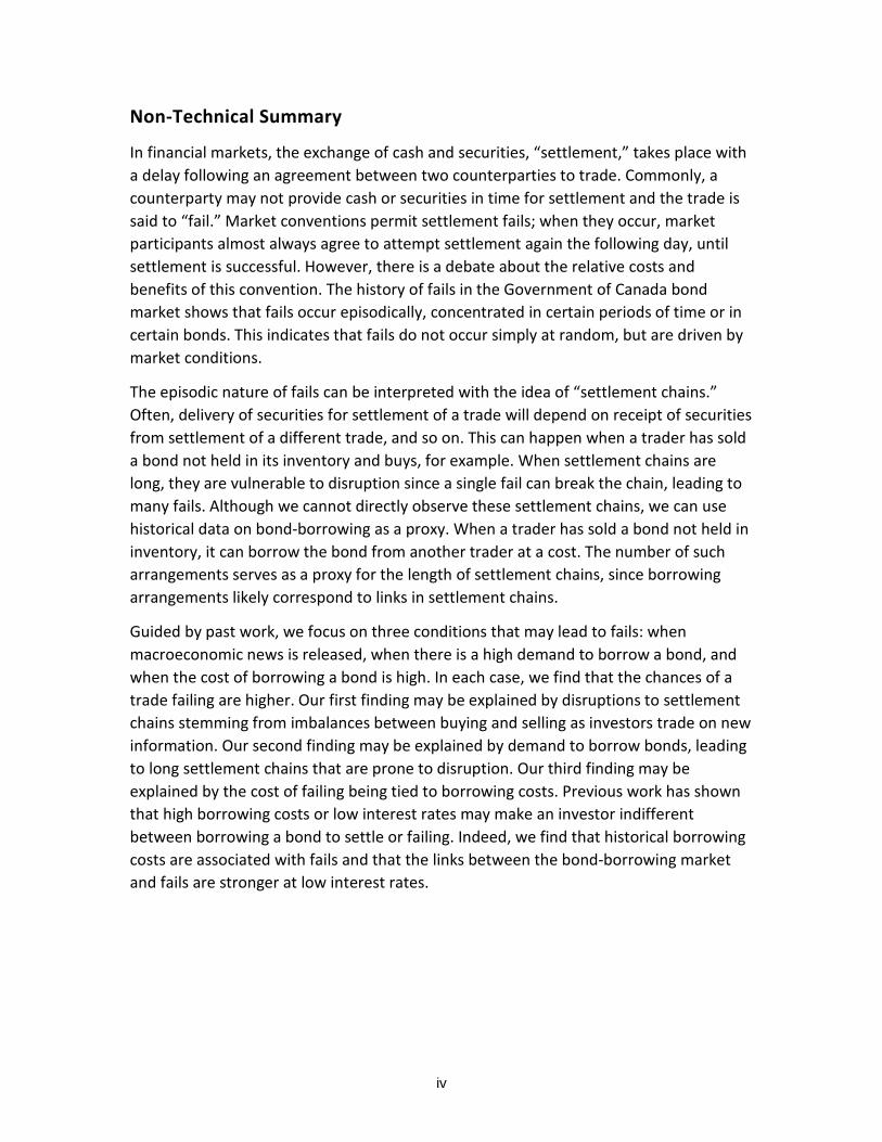
In financial markets, the exchange of cash and securities, “settlement,” takes place with a delay following an agreement between two counterparties to trade. Commonly, a counterparty may not provide cash or securities in time for settlement and the trade is said to “fail.” Market conventions permit settlement fails; when they occur, market participants almost always agree to attempt settlement again the following day, until settlement is successful. However, there is a debate about the relative costs and benefits of this convention. The history of fails in the Government of Canada bond market shows that fails occur episodically, concentrated in certain periods of time or in certain bonds. This indicates that fails do not occur simply at random, but are driven by market conditions.
The episodic nature of fails can be interpreted with the idea of “settlement chains.” Often, delivery of securities for settlement of a trade will depend on receipt of securities from settlement of a different trade, and so on. This can happen when a trader has sold a bond not held in its inventory and buys, for example. When settlement chains are long, they are vulnerable to disruption since a single fail can break the chain, leading to many fails. Although we cannot directly observe these settlement chains, we can use historical data on bond-borrowing as a proxy. When a trader has sold a bond not held in inventory, it can borrow the bond from another trader at a cost. The number of such arrangements serves as a proxy for the length of settlement chains, since borrowing arrangements likely correspond to links in settlement chains.
Guided by past work, we focus on three conditions that may lead to fails: when macroeconomic news is released, when there is a high demand to borrow a bond, and when the cost of borrowing a bond is high. In each case, we find that the chances of a trade failing are higher. Our first finding may be explained by disruptions to settlement chains stemming from imbalances between buying and selling as investors trade on new information. Our second finding may be explained by demand to borrow bonds, leading to long settlement chains that are prone to disruption. Our third finding may be explained by the cost of failing being tied to borrowing costs. Previous work has shown that high borrowing costs or low interest rates may make an investor indifferent between borrowing a bond to settle or failing. Indeed, we find that historical borrowing costs are associated with fails and that the links between the bond-borrowing market and fails are stronger at low interest rates.

1
1. Introduction
Trades in bond and stock markets are typically settled with a delay ranging from a few hours, in
the case of short-dated instruments, to a few days, in the case of longer-dated instruments.
Settlement of trades means that securities are delivered against cash or other securities. For
some trades, securities are not delivered at the expected settlement date. These settlement
fails—or just “fails”—are common in bond and stock markets.
A debate persists around the relative costs and benefits of fails. For instance, constraints on
settlement fails may restrict short-selling activities, which are important to support price
efficiency and market liquidity (Liu, McGuire, Swanson 2016; Fotak, Raman, Yadav 2014).
However, settlement fails can also be disruptive if they lead to a reluctance to trade or result in
large, unanticipated outstanding counterparty exposures.
Our focus is different. We investigate the underlying determinants of fails in the fixed-income
market, where there is little existing evidence. Preliminary evidence suggests that fails in fixed
income are concentrated in the most liquid and largest issues, such as benchmark bonds, which
we confirm in our data. This contrasts with the equity markets where the stocks of smaller and
less-known companies are harder to borrow and may be more likely to have fails (D’Avolio
2002). Our analysis focuses on the Canadian government bond market where we can compile a
unique and comprehensive dataset covering trades, settlements and fails, for both the bond
and repo markets.
As a motivation for our analysis, we first test the simplest explanation for fails. Fails may be
independent events, akin to accidents. In other words, each trade fails with a fixed probability,
independently of other trades. This hypothesis is rejected in the data. Starting with observed
trades, we generate a simulated distribution of failed trades using the assumption that each
trade fails independently of others and with fixed probability. The simulated distribution of fails
is different from the observed distribution. Days with very low volume of fails and days with
very high volume of fails are much more frequent in the data than in our simulated distribution.

2
We investigate the determinants of fail episodes in the Canadian fixed-income markets. In all of
our tests we include bond characteristics as control variables, such as the outstanding quantity,
age, and benchmark status. Our focus is changes in the market conditions that may drive fail
episodes. The evidence is consistent with fails cascading through “settlement chains.”
Settlement chains are formed when a bond can be recirculated through a series of transactions
in the cash and repo markets. For instance, consider a short-seller who borrows a bond from a
bond owner to settle a sale. The buyer in this transaction is now a bond owner who can again
lend this bond—perhaps to raise funds for his purchase.
First, we find that the likelihood and the magnitude of settlement fails are larger following
macroeconomic news releases. Economic news events are closely watched by bond investors
and have a significant impact on bond yields. New information leads some bond owners to
change their portfolio allocation. These purchases and sales, if widespread, may break links in
settlement chains as bond lenders recall their loans to meet delivery obligations, increasing the
chances of settlement fails. We find larger effects for negative economic news. Since negative
news is typically associated with lower yields and higher prices, this is consistent with scarcity
increasing the chance of settlement fails.
Second, we find that fails increase with trading activity in the borrowing market. The link
between fails and the bond-borrowing market is also consistent with the existence of
settlement chains. The details of these settlement chains are unobservable but they can be
proxied using a bond’s “velocity,” where velocity is the amount of bonds on loan relative to the
quantity of bonds available for trading.
Third, we find that fails increase with the cost of borrowing a bond, either on the securities
lending market or the repo market. We also find that the sensitivity of settlement fails to
borrowing activity and borrowing costs are larger when the level of interest rate is lower.
Together, this evidence suggests that lower opportunity costs play a significant role in the
likelihood and the size of fails. The opportunity cost from failing to deliver a bond is the forgone
interest rate on the cash that is not received (when settlement fails). This opportunity cost
decreases as the bond-specific borrowing cost increases and it also increases as the general
level of interest decreases (e.g., see Fleming, Garbade 2005; Fontaine, Hately, Walton 2017).

3
The evidence suggests that the lower opportunity costs act as a friction preventing adjustments
to the market price that would clear demand and supply of specific bonds.
Settlement chains provide a useful and intuitive way to interpret our results. But our findings
do not depend on the existence of settlement chains. This is important since we do not observe
settlement chains directly. We cannot tell whether a few fails affect one long and complex
chain or whether many correlated fails affect several shorter, simpler chains.
Our results from the Canadian market may carry important implications for markets in other
jurisdictions with similar institutional features. Several features of the Canadian government
bond market are like other securities markets: market conventions for settlement fails;
staggered settlement; the role of the repo market in borrowing bonds to settle short sales in
fixed-income markets; and the cost of failing being tied to the level of interest rates.
One important question is whether market quality and allocational efficiency worsen for bonds
with greater likelihood and magnitude of fails. We leave this for future research. Nonetheless,
our results carry important implications for policy-makers. We find that the relationships
between bond characteristics and fails have the expected signs. For instance, settlement fails
are less likely for bonds issued recently or with larger issue. Nonetheless, fails happen more
frequently on days with new economic information, when the level of interest rate is low and
when a bond becomes expensive to borrow. This suggests that restoring the opportunity costs
of fails can substantially reduce the likelihood and the magnitude of settlement fails, especially
at times when investors are trading on economic news, or when interest rates are very low or
negative. Indeed, restoring the price mechanism in the borrowing market via the introduction
of a fails charge in the US market for Treasury and agency mortgage-backed bonds seems to
have reduced fails (Fleming, Garbade 2005).
i. Related literature Empirical work on fixed-income fails is limited. Corradin and Maddaloni (2015) find that central
bank purchases are associated with fails in the Italian bond and repo market. Other existing
results focus on equity markets, but these results neglect the role of economic news on fails.
Boni (2006) shows that fails increase when borrowing fees increase. Higher levels of fails in the

4
equity market may result in mispricing and increased volatility (Stratmann, Welborn 2012;
Autore, Boulton, Braga-Alvesc 2014), but the evidence is mixed. Raising the costs of a
settlement fail—to control the quantity of fails—may act as a constraint on short-selling and
may reduce market liquidity and price discovery (Liu, McGuire, Swanson 2016; Fotak, Raman,
Yadav 2014). Market-makers in equity options may also benefit from the possibility of failing
and their associated costs affect option prices (Evans, Geczy, Musto, Reed 2005).
2. Settlement of transactions and settlement fails in the bond market
This section details the settlement of transactions in the Canadian bond market and, in
particular, the events that occur when there is a settlement fail. This description is useful for
understanding how fails happen.
i. Transaction settlement in the bond and repo market In Canada, as in most bond markets, the settlement of cash fixed-income transactions is usually
deferred until a few days after a trade is negotiated. To illustrate, the price and quantity of
bonds to be exchanged are agreed at time t, but no exchange of bonds and cash occurs at time
t. Instead, the seller will deliver bonds to settle the transaction in exchange for cash at time
t + 3.2
In contrast, the repo market has a same-day settlement convention; trades are agreed and
settled on the same day. Therefore, a seller in the cash market at time t can use the repo
market to borrow the bond using a reverse repo transaction at time t+1, t+2 or t+3 to settle its
transaction. One important benefit from deferred settlement in the cash market is that market
participants may sell bonds that they do not hold in inventory at time t. For instance, a dealer
2 By convention, settlement occurs at t+3 for Government of Canada bonds with maturity greater than three years and at t+2 for bonds with maturity less than three years. Money market instruments including repos settle on the day of trade. As of 5 Sept 2017, Canadian and US markets moved to a t+2 settlement cycle for markets that weren’t already settling at t+2 or earlier: www.cds.ca/newsroom?id=161.

5
may sell a bond to provide liquidity to a client or to establish a short position (to benefit
interest rates rising) and then enter into repo transactions at later dates to obtain securities.
ii. Failure to deliver bonds during transaction settlements But what happens if a short-seller or a market-maker does not deliver bond at t+3 to settle the
transactions? By design, the bond market does not stigmatize settlement fails. Instead, the
counterparties can agree (and almost always agree) to delay settlement by one day, keeping
the initial terms unchanged. Therefore, any capital gain or loss due to a change in yield is still
computed relative to the time-t price. However, failing to deliver a bond still carries a cost: the
party that fails to deliver securities does not receive cash and forgoes interest at t+3. The party
delivering cash can keep the cash and earn interest until settlement is successful.
Settlement fails in repo transactions are handled similarly. Repo transactions specify a time and
price at which bonds and cash must be exchanged. Again, failing to return the bond is not
stigmatized. Both parties can agree to roll over the repo transactions by one day, but keep the
initial terms unchanged. In this case, failing to deliver a bond has the opportunity cost of
forgone interest rates.
3. Hypotheses
This section details three hypotheses at the core of the paper. These three hypotheses propose
distinct economic determinants that increase the likelihood and magnitude of settlement fails.
These determinants are also discussed in Fontaine, Hately and Walton (2017).
i. Economic surprises and settlement fails Settlement chains are not static. At any point in time, investors—long or short—may choose to
reverse their position. For instance, some long investors can decide to sell their bonds. To
execute this sale, the investors must recall the bonds that they own but had lent. This forces
their counterparts to search for bonds available for lending, which leads to Hypothesis I.

6
Hypothesis I
The likelihood and magnitude of bond settlement fails are greater following significant economic news surprises.
Investors assess the new information contained in economic surprises. Therefore, the surprises
can lead to a large reallocation of bonds between buyers and sellers if the news leads them to
reassess the value of their bond holdings. If a large number of sellers recall securities they have
lent as a result of the information release (i.e., economic surprise), several links in settlement
chains may be removed. To restore the settlement chain, the borrowers of bonds that face a
recall must borrow again from another bond owner, or another set of bond owners.
Hypothesis I predicts a larger likelihood that at least one recall will fail to settle and cascade
through the settlement chains.
ii. The borrowing market and settlement fails Bonds with relatively high trading volume in the cash market tend to have a large stock on loan
(either via the repo or securities lending market; see, e.g., Bulusu, Gungor 2017). This happens
mechanically, as market-makers and short-sellers borrow bonds to settle a large volume of cash
market transactions. In turn, the buyer in the cash market can make this bond available for
lending again. For instance, this buyer may use a repo transaction to finance the position.
Because of staggered settlement (see section 1), the same bond can circulate through a chain
of repo and cash transactions. This leads to our second hypothesis.
Hypothesis II
The likelihood and magnitude of bond settlement fails are greater for bonds with higher velocity.
The existence of settlement chains has an important consequence. Not all counterparties along
settlement chains hold the bond in their inventory. The bond instead passes from one investor
to another until it reaches its final owner. We refer to the length and number of settlement
chains as a bond’s velocity. Velocity captures the idea that the number of settlement claims can
outnumber the quantity of bonds available for trading. When velocity increases, isolated fails
can cascade through the settlement chain. Of course, it could be that there is no settlement
chain. In this case, statistical tests should reject Hypothesis II.
7
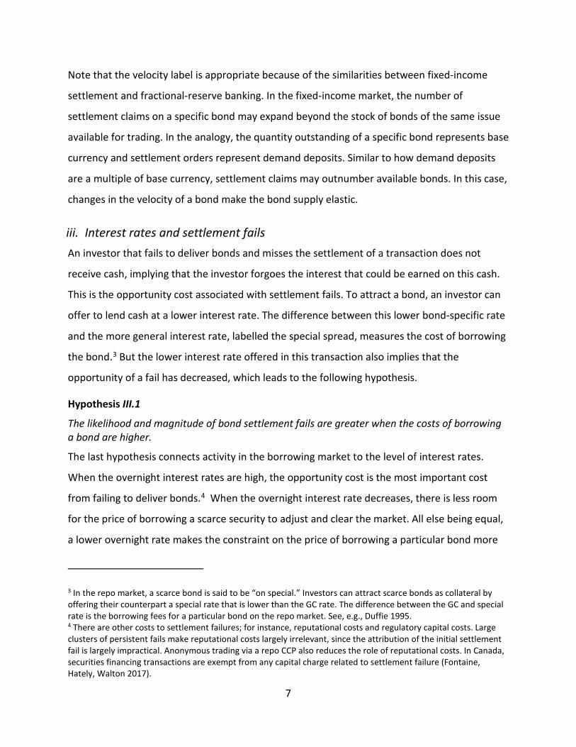
Note that the velocity label is appropriate because of the similarities between fixed-income
settlement and fractional-reserve banking. In the fixed-income market, the number of
settlement claims on a specific bond may expand beyond the stock of bonds of the same issue
available for trading. In the analogy, the quantity outstanding of a specific bond represents base
currency and settlement orders represent demand deposits. Similar to how demand deposits
are a multiple of base currency, settlement claims may outnumber available bonds. In this case,
changes in the velocity of a bond make the bond supply elastic.
iii. Interest rates and settlement fails An investor that fails to deliver bonds and misses the settlement of a transaction does not
receive cash, implying that the investor forgoes the interest that could be earned on this cash.
This is the opportunity cost associated with settlement fails. To attract a bond, an investor can
offer to lend cash at a lower interest rate. The difference between this lower bond-specific rate
and the more general interest rate, labelled the special spread, measures the cost of borrowing
the bond.3 But the lower interest rate offered in this transaction also implies that the
opportunity of a fail has decreased, which leads to the following hypothesis.
Hypothesis III.1
The likelihood and magnitude of bond settlement fails are greater when the costs of borrowing a bond are higher.
The last hypothesis connects activity in the borrowing market to the level of interest rates.
When the overnight interest rates are high, the opportunity cost is the most important cost
from failing to deliver bonds.4 When the overnight interest rate decreases, there is less room
for the price of borrowing a scarce security to adjust and clear the market. All else being equal,
a lower overnight rate makes the constraint on the price of borrowing a particular bond more
3 In the repo market, a scarce bond is said to be “on special.” Investors can attract scarce bonds as collateral by offering their counterpart a special rate that is lower than the GC rate. The difference between the GC and special rate is the borrowing fees for a particular bond on the repo market. See, e.g., Duffie 1995. 4 There are other costs to settlement failures; for instance, reputational costs and regulatory capital costs. Large clusters of persistent fails make reputational costs largely irrelevant, since the attribution of the initial settlement fail is largely impractical. Anonymous trading via a repo CCP also reduces the role of reputational costs. In Canada, securities financing transactions are exempt from any capital charge related to settlement failure (Fontaine, Hately, Walton 2017).

8
likely to bind. Hence, we expect the relationship between fails and borrowing costs and as well
as between fails and velocity to strengthen as the overnight rate decreases.
Hypothesis III.2
The relationship between fails and activity in the borrowing market is stronger when the level of the overnight interest rate is lower.
It is true that we should expect a more direct relationship between fails and the overnight rate,
since the opportunity costs of settlement fails decrease with the level of interest rate (Fleming,
Garbade 2005; Fontaine, Hately, Walton 2017). We do not test this direct channel since the
variations of the overnight rate are not sufficient in our sample.
4. Bond data
We merge several sources to construct a panel dataset. Our sample runs from October 2014 to
February 2017. The beginning of our sample is dictated by data availability. This period exhibits
large variations in settlement fails, both across bonds and over time, which we describe below.
The unit of our dataset is bond-days. For each day, we identify the ISIN of all outstanding
Government of Canada nominal bonds denominated in Canadian dollars using a dataset from
Thomson Reuters. We ignore inflation-linked bonds owing to low trading volume. We ignore
Treasury bills, since they are settled on the same date as they are traded. We then collect a rich
set of market information about these bonds. Table 1 lists key variables and data sources,
which we describe below.
Table 1: Description of variables. Short name Description Unit Source
Velocity Securities on loan as a share of float % Markit
Borrowing Fee Securities lending fee Bps Markit
Repo Spread BoC target rate minus special repo rate Bps CDCC
Log Volume Log daily settlement volume Log-millions CDS
Log Float Log of float Log-millions Thomson Reuters
Age Time since issuance Years CDS
GC Bank of Canada target GC rate Bps Bank of Canada

9
Yield Yield to maturity % DEX
Benchmark Benchmark status dummy [0,1] Bank of Canada
Pre-benchmark Pre-benchmark status dummy [0,1] Bank of Canada
i. Outstanding amount data We collect data on bonds’ outstanding amount from Thomson Reuters DataScope. We use the
outstanding amount as a proxy for the quantity of bonds available for trading. We refer to the
outstanding amount as the “float.”
ii. Trade settlement data We merge our universe of nominal bonds with two datasets from the Canadian securities
clearing and settlement authority, the Canadian Depository for Securities (CDS). The first
dataset is commercially available and contains settlement orders related to Canadian fixed-
income securities. Each settlement order is generated by an underlying trade. For each trade,
we collect the ISIN of the bond, the par value of the settlement order, and the planned
settlement date and whether the trade generated the settlement order. Trades that were part
of a repo are flagged; we refer to all non-repo trades as “cash trades.”
In the case of a cash trade, we observe a single settlement order. In the case of a repo trade,
we observe two settlement orders: the first order is for the initial exchange of securities for
cash, and the second order represents the return of the bond in exchange for principal and
interest. We refer to this dataset as the “trades” dataset.
iii. Settlement fails data The second dataset from CDS contains information about settlement fails for each bond and for
each day. Each record represents a settlement order that failed. For each settlement fail, we
collect the bond ISIN, the par value to settle, the planned settlement date and whether the
underlying trade was a cash or repo trade. We refer to this dataset as the “fails” dataset. Note
that we can identify new versus old fails.5 The data include settlement fails that appeared
5If the settlement fail date occurs after the planned settlement date, then this trade had failed on a prior date and failed again at a new delivery attempt. We deem the settlement failure an “old” fail in this case.

10
unresolved for long periods of time. We attribute these to data errors and we exclude
observations of settlement fails that have been outstanding for more than five days.
iv. Settlement volume We merge the trades and fails dataset by ISIN to compute the total par value of each bond due
to be settled on each date. From the trades dataset, we observe all new settlement orders
generated by trading activity. From the fails dataset, we observe past settlement orders that
failed in the past and that will be attempted again. For each bond-day in our sample,
settlement volume is the sum of new settlement orders and older failed settlement orders. We
will refer to the terms “settlement volume” and “volume” interchangeably. The appendix
details the construction of the settlement volume series.
iv. GC and special repo rates data We collect data from the Canadian Derivatives Clearing Corporation (CDCC), which provides
central clearing services for a segment of the Canadian repo market. The dataset includes
trade-by-trade data on repo trades that are cleared through CDCC. The data include the
accrued interest of each trade from which we compute the daily average specific repo rate for
each ISIN. We also compute the specific repo spread by subtracting the specific repo rate from
the Bank of Canada’s target overnight interest rate.
v. Bond yields We collect data from the FTSE TMX on daily bond yields. The dataset provides end-of-day yields
for each bond in our dataset, which are computed from daily information provided by fixed-
income dealers. We ignore observations of yield with less than 30 days to maturity since they
are sensitive to small deviations from the theoretical price.
vi. Securities lending data We collect data from the Markit Securities Finance dataset. This dataset provides securities
lending information. For each bond ISIN and for each day, we collect the total par value on loan.
Our proxy for the velocity of a bond is the ratio of this quantity of bond on loan to the quantity
of bond outstanding (i.e., the float). This share of the outstanding bond takes a value between 0

11
and 1 by construction. We also collect the average borrowing fee for new loans over the past
three days, weighted by the par value of each security loan.
Table 2 reports summary statistics for key variables describing bond characteristics and pricing
information.
Table 2: Summary statistics—bond-level information. The table shows summary statistics for bond-level variables over the sample period. The columns show the mean and standard deviation (Mean and Std.); 25th, 50th and 75th percentiles (25%, 50% and 75%); and the number of observations (N). The results are split by benchmark and non-benchmark bonds across the upper and lower panels.
Mean Std. 25% 50% 75% N Benchmark bonds
Log Fails 4.15 2.40 3.00 4.66 5.80 939 Velocity 22.98 9.41 17.05 21.53 27.62 1787 Borrowing Fee 10.07 4.72 7.42 8.52 10.88 1777 Repo Spread 12.74 13.14 2.93 8.16 18.35 911 Log Volume 9.64 0.57 9.44 9.68 9.91 1785 Log Float 9.49 0.18 9.27 9.51 9.62 1787 Age 0.82 0.45 0.41 0.74 1.23 1787 Yield 0.99 0.43 0.62 0.88 1.34 1772
Non-benchmark bonds Log Fails 2.32 2.69 0.40 2.71 4.48 5485 Velocity 11.53 7.44 6.73 10.51 14.47 25206 Borrowing Fee 10.43 5.92 7.30 8.65 11.86 20061 Repo Spread 9.56 11.39 2.04 5.68 11.38 9660 Log Volume 6.85 1.95 6.39 7.37 8.02 24185 Log Float 8.89 1.04 8.94 9.23 9.48 25206 Age 7.25 7.63 1.93 3.98 9.34 25206 Yield 1.04 0.58 0.57 0.83 1.41 24612
vii. Macroeconomic news We construct an index of macroeconomic surprises. First, we collect the following economic
releases: consumer price index (CPI), payroll survey, real gross domestic product (GDP), retail
sales, and unemployment. Second, for each of these variables, we also obtain from Bloomberg
the analysts’ forecast and subtract it from the released data to compute the surprise
component. Third, we normalize each variable to have a mean of 0 and a standard deviation of
1 on the days of their release. Our news index is the daily sum of the absolute normalized
surprises. Implicitly, we assume each component of the index is equally important. Figure 1
reports this Canadian index of macroeconomic surprises.

12
Figure 1. Canadian macroeconomic news index. Index of Canadian macroeconomic surprises for CPI, payroll survey, real gross domestic product, retail sales, and unemployment. We compute the surprise as the difference between each of the economic releases minus the corresponding survey forecast from Bloomberg, normalized to a standard deviation of 1. The macroeconomic news index is the sum of the absolute value of surprises.
5. Are settlement fails random?
Could settlement fails be unrelated to each other? In other words, is it the case that a given
trade may fail to settle with fixed probability, independently from any other trades? This is the
simplest hypothesis. If this is the case, the volume of fails should be a constant proportion of
the settlement volume (on average). This hypothesis can be tested with the following
simulation. For each trade in our sample during the 2015 calendar year, we assigned a
simulated failed variable taking values 0 or 1 with probability p or 1-p, respectively (i.e., a
Bernoulli random variable).6 The probability p is calibrated so that the empirical mean of the
fraction of trading volume that fails matches the simulated fraction of trading volume that fails.
Given that the simulated mean matches the observed mean, we can then ask whether the
distribution also matches.
6 We have used a subset of our sample dates in this case to balance the number of sample size with the computational ease of a smaller trade-by-trade dataset.
13
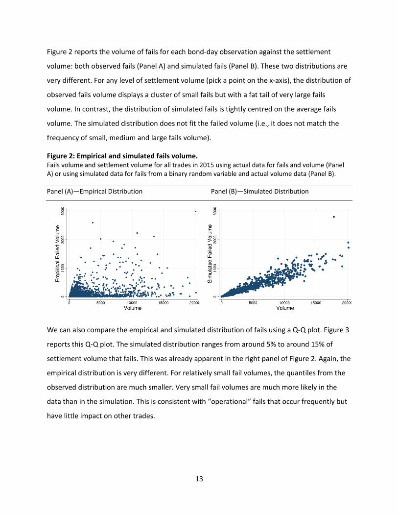
Figure 2 reports the volume of fails for each bond-day observation against the settlement
volume: both observed fails (Panel A) and simulated fails (Panel B). These two distributions are
very different. For any level of settlement volume (pick a point on the x-axis), the distribution of
observed fails volume displays a cluster of small fails but with a fat tail of very large fails
volume. In contrast, the distribution of simulated fails is tightly centred on the average fails
volume. The simulated distribution does not fit the failed volume (i.e., it does not match the
frequency of small, medium and large fails volume).
Figure 2: Empirical and simulated fails volume. Fails volume and settlement volume for all trades in 2015 using actual data for fails and volume (Panel A) or using simulated data for fails from a binary random variable and actual volume data (Panel B).
Panel (A)—Empirical Distribution Panel (B)—Simulated Distribution
We can also compare the empirical and simulated distribution of fails using a Q-Q plot. Figure 3
reports this Q-Q plot. The simulated distribution ranges from around 5% to around 15% of
settlement volume that fails. This was already apparent in the right panel of Figure 2. Again, the
empirical distribution is very different. For relatively small fail volumes, the quantiles from the
observed distribution are much smaller. Very small fail volumes are much more likely in the
data than in the simulation. This is consistent with “operational” fails that occur frequently but
have little impact on other trades.

14
Figure 3: Q-Q Plot of empirical and simulated fails volume.
In contrast, for relatively large trades, the quantiles of observed fails are much larger than in
the simulation simulated. For a significant number of bond-day observations, there is a large
share of volume fails. Observed fails range as high as 100% of settlement volume.
Table 3 reports summary statistics for empirical and simulated data. The means are essentially
the same by construction—close to 8%. However, a two-sample Kolmogorov-Smirnov test for
equality of distribution functions yields a p-value of essentially 0, rejecting that the distributions
are equal. The empirical distribution is very asymmetric. The median share of fails volume is 2%,
much smaller than the mean. The tails are much larger, with kurtosis 16 compared with a
kurtosis of 4 for the simulated distribution.
Table 3: Summary statistics for empirical distribution of fails. Mean Median Std. Skewness Kurtosis N
Empirical 7.71% 2.31% 13.75% 3.31 16.37 1930
Simulated 7.77% 7.64% 1.93% 0.79 4.10 1930
Our findings are consistent with settlement chains from the recirculation of bonds driving the
correlation between failed trades. Settlement chains explain why a small probability of fails for
15
individual trade—the median share of volume that fails is less than 2%—can also explain cases
where a large share of volume can fail on some bond-day. In some cases, settlement fails are
highly correlated across trades.
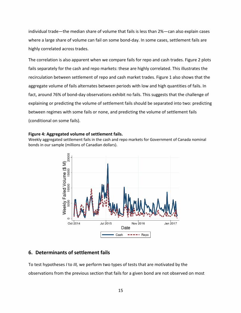
The correlation is also apparent when we compare fails for repo and cash trades. Figure 2 plots
fails separately for the cash and repo markets: these are highly correlated. This illustrates the
recirculation between settlement of repo and cash market trades. Figure 1 also shows that the
aggregate volume of fails alternates between periods with low and high quantities of fails. In
fact, around 76% of bond-day observations exhibit no fails. This suggests that the challenge of
explaining or predicting the volume of settlement fails should be separated into two: predicting
between regimes with some fails or none, and predicting the volume of settlement fails
(conditional on some fails).
Figure 4: Aggregated volume of settlement fails. Weekly aggregated settlement fails in the cash and repo markets for Government of Canada nominal bonds in our sample (millions of Canadian dollars).
6. Determinants of settlement fails
To test hypotheses I to III, we perform two types of tests that are motivated by the
observations from the previous section that fails for a given bond are not observed on most

16
days, and that the failed volume varies widely when fails occur. In all of our tests, we include
the age of a bond, the quantity outstanding and a dummy for benchmark bonds in our control
variables.
Formally, we follow the two-stage approach proposed in Duan et al. (1983) for analyzing data
with observations bounded below at 0. In the first stage, we use a logit model to consider the
determinants of the likelihood that any fails occur on a bond-day observation. We consider fails
in either cash or repo since they are highly correlated, as shown in Figure 4. In the second stage,
we use linear ordinary least squares (OLS) to consider the determinants of the volume of fails,
conditional on the event that some fails occur in a bond-day observation.
We estimate logit models of the following form:
𝑓𝑓𝑓𝑓𝑓𝑓𝑓𝑓𝑓𝑓𝑓𝑓𝑖𝑖,𝑡𝑡 = �1 𝑓𝑓𝑓𝑓 𝑦𝑦𝑖𝑖,𝑡𝑡 > 00 otherwise
𝑓𝑓𝑓𝑓𝑓𝑓𝑓𝑓𝑓𝑓𝑓𝑓𝑖𝑖,𝑡𝑡 = 𝛽𝛽𝐵𝐵𝑖𝑖,𝑡𝑡 + 𝛼𝛼 𝑋𝑋𝑖𝑖,𝑡𝑡 + 𝛾𝛾 𝐹𝐹𝐹𝐹𝑖𝑖 + 𝜀𝜀𝑖𝑖,𝑡𝑡,
where 𝑓𝑓𝑓𝑓𝑓𝑓𝑓𝑓𝑓𝑓𝑓𝑓𝑖𝑖,𝑡𝑡indicates whether bond i exhibits at least one failed trade on day t (𝑦𝑦𝑖𝑖,𝑡𝑡 > 0).
𝐵𝐵𝑖𝑖,𝑡𝑡 is a vector of variables that varies depending on the hypothesis being tested, including:
macroeconomic news surprises and yield changes (Hypothesis I); a bond’s velocity (Hypothesis
II); a bond’s borrowing fee and repo spread (Hypothesis III.1); and the level of interest rates
(Hypothesis III.2). The coefficient of interest is 𝛽𝛽. The set of control variables 𝑋𝑋𝑖𝑖,𝑡𝑡 includes the
logarithm of settlement volume for bond i on day t, its age, the float outstanding, and constant
dummy variables indicating whether a bond is in the pre-benchmark or benchmark stage to
control for bonds’ life cycle effects. In all our results, the estimated coefficients for these
control variables have the expected sign, although always statistically significant.
We estimate the magnitude of failed settlements, conditional on at least one fail, in a linear OLS
model:
𝑓𝑓𝑓𝑓𝑓𝑓𝑓𝑓 𝑣𝑣𝑣𝑣𝑓𝑓𝑣𝑣𝑣𝑣𝑓𝑓𝑖𝑖,𝑡𝑡�𝑓𝑓𝑓𝑓𝑓𝑓𝑓𝑓𝑓𝑓𝑓𝑓𝑖𝑖,𝑡𝑡 = 𝛽𝛽𝐵𝐵𝑖𝑖,𝑡𝑡 + 𝛼𝛼 𝑋𝑋𝑖𝑖,𝑡𝑡 + 𝛾𝛾 𝐹𝐹𝐹𝐹𝑖𝑖 + 𝜀𝜀𝑖𝑖,𝑡𝑡,

17
where 𝑓𝑓𝑓𝑓𝑓𝑓𝑓𝑓 𝑣𝑣𝑣𝑣𝑓𝑓𝑣𝑣𝑣𝑣𝑓𝑓𝑖𝑖,𝑡𝑡 is the logarithm of bond i’s total failed volume on day t. All other
variables are as above; the coefficient of interest is 𝛽𝛽. In all regressions, we estimate panel
models with bond fixed effects and we estimate standard errors clustered by bond and by date.
i. Economic surprises (Hypothesis I) Hypothesis I predicts that economic surprises lead to a larger likelihood of fails and larger failed
volume. We use a logit regression to model the likelihood that any fails occur on a bond-day
observation and we use a linear OLS model to analyze the determinants of failed volume. The
results support Hypothesis I.
Table 4 reports results for logit and OLS models where we include the contemporaneous news
index and its first lag. Including only one lag is optimal based on the Bayesian information
criterion. We estimate the models with and without control variates for robustness. The
coefficients on certain control variates are suppressed for brevity. First, controlling for
economic surprises, we find that velocity, specialness and volume are each significant
determinants of the likelihood and magnitude of fails (this is discussed further in the following
sections). Second, economic surprises significantly increase the likelihood of fails, but do not
influence the volume failed (again, conditional on some fails occurring). Increased likelihood of
fails is associated with Lag News, possibly because of hedging positions taken in the cash
market before announcement dates that are due to settle after announcement dates. The
coefficient estimates for Lag News are economically significant; the model indicates that when
economic surprises range from their lowest to highest sample decile, the probability of a fail
occurring the day after a surprise increases by around 10%, holding all other variables at their
sample means.

18
Table 4: Economic surprises and fails. Logit model for the likelihood of fails as well as OLS linear regression of fail volume with economic surprises. Every regression includes bond fixed effects. Standard errors are clustered by bond and date.
(OLS 1) (OLS 2) (Logit 1) (Logit 2) News 0.0378 -0.0207 -0.0233 -0.0220 (0.43) (-0.29) (-0.67) (-0.58) Lag News 0.136 0.0901 0.102*** 0.124*** (1.35) (0.99) (3.61) (3.83) Velocity 0.0254* 0.0168*** (1.86) (2.61) Borrowing Fee
0.0426*** 0.0183***
(3.18) (4.21) Log Volume 0.435*** 0.200*** (5.35) (3.18) Controls No Yes No Yes Obs. 6420 6084 26753 21615 Adj., Pse. R2 0.151 0.200 0.115 0.093
Panel (A) of Table 5 reports results from an extended version of the model and includes bond-
specific absolute value of change in yield on a day with economic surprises. The size of an
economic surprise is an incomplete measure for its effect on the bond market. Other factors
affect how investors respond to new information. The change in the yield of bond i following an
economic surprise provides a more direct measure. As expected, the results are stronger when
using a more direct proxy for the effect of news on yields. The evidence shows that a given
bond is more likely to fail and that its failed volume is larger when its yield shows a larger
change around economic news.

19
Table 5: Economic surprises, yield changes, and fails. Logit model for the likelihood of fails as well as OLS linear regression of fail volume. The variable Diff|Y| is the change in the yield of bond i on date t (in absolute value) on a day with economic surprises. The variable Diff| Ŷ | is the predicted yield changes based on a regression of yield changes on surprises. Every regression includes bond fixed effects. Standard errors are clustered by bond and date.
Panel A—Regressions with actual yield changes (Logit 1) (Logit 2) (OLS 1) (OLS 2) Diff |Y| 0.249 -0.0314 6.213* 2.506 (0.12) (-0.02) (1.71) (0.86) Lag diff |Y| 4.589** 4.801*** 11.35*** 8.093*** (2.54) (2.63) (3.65) (2.83) Controls No Yes No Yes N 26753 21615 6420 6084 Adj., Pse. R2 0.115 0.093 0.154 0.201
Panel B—Regressions with predicted yield changes (Logit 1) (Logit 2) (OLS 1) (OLS 2) Diff | Ŷ | -2.066 -3.946 13.56 6.570 (-0.37) (-0.68) (1.11) (0.71) Lag diff | Ŷ | 20.87*** 20.14*** 20.96 13.89 (4.32) (4.12) (1.64) (1.30) Controls No Yes No Yes N 26753 21615 6420 6084 Adj., Pse. R2 0.115 0.094 0.152 0.200
One concern with Panel (A) is that part of the results may be owing to fails causing yield
changes (in addition to economic surprises causing fails). The observation that lagged yield
changes explain fails should help to alleviate this concern. In addition, we can proceed with a
two-stage estimator in the following way. In a preliminary step, we project yield changes on
contemporaneous economic surprises, where we also include control variables about bond
characteristics and trading activity. In the second step, we use the absolute value of the
predicted yield changes in the regressions.
Panel (B) of Table 5 reports the results. The evidence provides two messages. First, yield
changes that can be attributed to economic surprises are associated with a greater likelihood of
fails. The coefficient estimates are larger and statistically significant. Second, predicted yield
changes are also positively associated with failed volume but the estimates are not statistically
significant.

20
For the OLS model of expected fails volume, we can modify our approach to obtain a two-stage
least squares (2SLS) instrumental variable regression where we use economic surprises as
instruments to estimate the effect of yield changes on fails. We split economic surprises
between good and bad economic news. Positive inflation, retail sales or payroll surprise news
as well as negative unemployment surprises are considered good economic news.
Table 6 reports the results of the 2SLS approach. Panel (A) reports results from first-stage
regressions of yield changes on either the positive or the negative component of economic
surprises. These regressions are estimated including controls for the other component of
economic surprises; we include the negative component of economic surprises in the
regression when we are interested in the positive component of economic surprises and vice
versa.7 The first two specifications (corresponding to the positive component of economic
surprises) have Kleibergen-Paap F-statistics of around 4, indicating we cannot reject the null
hypothesis that these are weak instruments. However, third and fourth specifications
(corresponding to the negative component of economic surprises) have Kleibergen-Paap and
Cragg-Donald F-statistics of greater than 15, allowing us to reject the null hypothesis that the
maximum relative bias of our instrumental variables regression is greater than 10%.
Individually, negative CPI and GDP surprises have significant coefficient estimates. Payroll and
Unemployment have insignificant coefficients, but these data are released on the same day.
Panel B reports results from the second-stage regressions of fail volume. The coefficient
estimates have a magnitude similar to the results shown in Table 5. In addition, the estimates
for negative news surprises are economically and statistically significant. A one-standard-
deviation change in yield predicted by a negative economic surprise results in an increase in
settlement fails in a single bond by around $40M when failed volume is at its sample mean and
conditional on a fail occurring.
Overall, the evidence in Tables 4 to 6 supports our main message: economic surprises cause an increase in the likelihood of settlement fails. The fact that negative economic surprises appear
7 Note that we account for the fact that payroll and unemployment are released on the same day. For instance, in a regression where the parameters of interest include the coefficient for positive payroll and unemployment surprises, we also include any negative payroll and unemployment surprises as control variables.

21
more important should be interpreted with care, since our sample is relatively short in the time-series dimension. Nonetheless, it is reassuring that the effect of news is more perceptible when bonds become more expensive; that is, when they are more difficult to find.
Table 6: The effect of yield changes on fail volume—instrumental variable regressions. Instrumental variable regressions of fail volumes (conditional on positive fail volume) on yield changes using economic surprises as instruments. First-stage regressions (Panel A) with and without bond-level controls. Second-stage regressions (Panel B) with and without bond-level controls.
Panel A—First stage Positive
surprises Positive surprises
Negative surprises
Negative surprises
CPI 0.00657 0.00644 0.0157*** 0.0168*** (1.13) (1.25) (2.87) (3.17) Payroll 0.0155 0.0160 0.00554 0.00526 (1.49) (1.46) (0.58) (0.54) GDP -0.00354 -0.00325 0.0270*** 0.0264*** (-0.21) (-0.20) (6.42) (5.89) Retail Sales 0.0146*** 0.0152*** 0.00812* 0.00765* (2.80) (3.31) (1.82) (1.88) Unemployment 0.00741 0.00758 0.00331 0.00287 (0.79) (0.81) (0.58) (0.51) Controls No Yes No Yes N 26061 21070 26061 21070 Adjusted R2 0.015 0.023 0.015 0.023
Panel B—Second stage Positive
surprises Positive surprises
Negative surprises
Negative surprises
Lag diff Ŷ 5.681 0.905 -17.63* -19.88*** (0.63) (0.12) (-1.76) (-2.65) Controls No Yes No Yes N 6263 5958 6263 5958 Adjusted R2 -0.016 0.065 -0.073 -0.018
ii. Explaining fails/no fails regimes (Hypotheses II and III.1) Table 7 reports results for logit regressions. Hypothesis II predicts that the likelihood of
settlement fails increases with a bond’s velocity. Hypothesis III.1 predicts that the likelihood of
fails increases with borrowing costs. The evidence supports these predictions using either the
borrowing fee or the repo spread as a proxy for the cost of borrowing a bond.

22
The results include coefficient estimates for velocity and borrowing costs with and without
controls for bond characteristics (i.e., age, issue size). Higher velocity or higher borrowing costs
increase the likelihood of settlement fails, either individually or combined with other controls.
The estimated effect of each variable is significant both statistically and economically. Using the
repo spread as a proxy for the costs of borrowing a bond reduces the sample size by half owing
to limited data, but the coefficient estimate is higher and has greater statistical significance.
Looking at the other coefficients, we find that bonds with larger trading volume are more likely
to fail. The age of a bond and the indicator for benchmark bonds also predict that fails are more
likely with significant estimates. In other words, for non-benchmark bonds, older bonds are
more likely to fail. The results show that the coefficients on issue size (float) are not significant.
In other words, controlling for indicators of scarcity and velocity, the issue size does not help
predict fails.
These results do not provide causal evidence between fails and velocity, but describe bond-
specific conditions that are associated with fails. We do not investigate multivariate time-series
dynamics.

23
Table 7: Fail/no fail regimes, velocity and borrowing costs. Logit regressions of the 𝑓𝑓𝑓𝑓𝑓𝑓𝑓𝑓𝑓𝑓𝑓𝑓𝑖𝑖,𝑡𝑡 indicator with value 1 when bond i exhibits at least one failed trade at date t; including bond fixed effects. Standard errors are clustered by bond and date.
(1) (2) (3) (4) (5) (6) (7) (8) Velocity 0.036*** 0.0176*** 0.0166*** 0.0214** (4.82) (2.59) (2.59) (2.22) Borrowing Fee
0.0159*** 0.0171*** 0.0182***
(3.28) (3.95) (4.20) Repo Spread
0.0347*** 0.0336*** 0.0333***
(7.17) (8.52) (9.02) Log Volume
0.141** 0.207*** 0.286*** 0.201*** 0.283***
(2.17) (3.34) (3.87) (3.22) (3.96) Log Float 0.447 0.321 0.191 0.243 0.126 (1.64) (1.11) (0.51) (0.91) (0.35) Benchmark 0.497*** 0.565*** 0.419*** 0.442*** 0.376 (2.75) (3.14) (1.77) (2.60) (1.52) Pre-Benchmark
-0.175 -0.224 -0.318 -0.253 -0.250
(-0.44) (-0.61) (-0.67) (-0.72) (-0.52) Age 0.0912 0.185** 0.307*** 0.161** 0.334** (1.07) (2.46) (2.07) (2.06) (2.34) N 26813 21717 10551 25927 21657 10551 21657 10551 Pseudo R2 0.120 0.076 0.095 0.118 0.092 0.109 0.093 0.110
Figure 5 illustrates the results of the model specified in columns (4) and (5) of Table 4. The
figure shows model-implied probabilities of fails for sample deciles of our variables of interest,
velocity and specialness. For example, the first sample decile for velocity for benchmark bonds
is around 12%. Evaluating the fitted logit model at this value and the sample means of all other
variables yields a probability of at least one fail of around 48%. The results are economically
significant. The model estimates indicate that when velocity changes from the lowest sample
decile to the highest, the probability of a fail increases by around 12% for benchmark bonds and
by around 5% for non-benchmark bonds, keeping all other variables at their sample means. For
specialness, model estimates indicate that an increase from the lowest sample decile to the
highest increases the probability of a fail occurring by around 4% for benchmark bonds and by
around 3% for non-benchmark bonds, keeping all other variables at their sample means.

24
Figure 5: Model probability of a fail occurring. The figure shows model values for the probability of a fail occurring in either the cash or repo market. Panel A corresponds to the model fit in specification (4) in Table 4, and Panel B corresponds to the model fit in specification (5) in Table 4. Points on the graph represent the probability of fails implied by the model when varying velocity (Panel A) or specialness (Panel B). The model is evaluated at each sample decile of velocity and specialness, holding all other variables constant at their sample means. Results are split into benchmark and non-benchmark bonds.
Panel (B)—Velocity Panel (B)—Specialness
iii. Explaining fails volume (Hypotheses II and III.1) Table 8 reports the results of benchmark OLS regressions of fails volume on velocity, proxies for
borrowing costs and other controls. Hypothesis II predicts that failed volume increases with a
bond’s velocity. Hypothesis III.1 predicts that failed volume increases with borrowing costs. The
results show that velocity and borrowing costs predict larger fails volume. As in the logit model,
these results do not provide causal evidence, but rather bond-specific conditions associated
with fails. The results are significant economically and statistically. Model specifications (1) and
(4) indicate that a one-standard-deviation increase in velocity results in an increase in failed
volume for a single bond by around $20M when failed volume is at its sample mean and
conditional on a fail occurring. Model specifications (2) and (5) indicate around the same
magnitudes for a one-standard-deviation increase in the borrowing fee.
Among other controls, bonds with larger trading volume have larger fails volume. In contrast
with the results for fails likelihood, the age of a bond predicts that fails volume is lower on

25
average for older bonds. The coefficient on velocity becomes insignificant when using repo
spread, but this is partly owing to the smaller sample. The issue size has the right sign but the
coefficient estimates are not significant.
Table 8: Fails volume, velocity and borrowing costs. OLS linear regressions of log fails volume for bond i at date t. Every regression includes bond fixed effects. Standard errors are clustered by bond and date.
(1) (2) (3) (4) (5) (6) (7) (8) Velocity 0.0336* 0.0243* 0.0260* 0.00763 (1.69) (1.73) (1.92) (0.38) Borrowing Fee
0.0558*** 0.0408*** 0.0426***
(3.71) (3.03) (3.20) Repo Spread 0.0513*** 0.0435*** 0.0434*** (6.91) (6.21) (5.15) Log Volume 0.480*** 0.448*** 0.770*** 0.433*** 0.768*** (5.77) (5.86) (6.66) (5.31) (6.65) Log Float -0.753 -0.617 -0.396 -0.689 -0.410 (-1.41) (-1.08) (-0.60) (-1.30) (-0.64) Benchmark 0.130 0.409 -0.401* 0.222 -0.414* (0.45) (1.40) (-1.66) (0.84) (-1.66) Pre-Benchmark
-0.738 -0.688 -0.479 -0.703 -0.446
(-0.93) (-0.88) (-0.77) (-1.01) (-0.73) Age -0.528*** -0.408*** -0.0731 -0.464*** -0.0635 (-4.83) (-3.87) (-0.30) (-4.32) (-0.27) N 6424 6088 2832 6424 6088 2832 6088 2832 Adjusted R2 0.156 0.147 0.225 0.214 0.197 0.255 0.199 0.255
iv. The level of interest rates (Hypothesis III.2) Hypothesis III.2 predicts that likelihood and the magnitude of fails are larger when interest
rates are lower. Unfortunately, the variations of the target rate are small in our sample. The
Bank of Canada target for the overnight rate covered only three values: 1%, 0.75% and 0.50%.
Therefore, we expect our tests to have small statistical power, since the variations in
opportunity costs of fails can be swamped by noise in the regression. The variations are also
infrequent. With only two changes in our sample, the changes in the GC rate can be swamped
by other slow-moving factors that affect market conditions (e.g., time-trend). Because of these
limitations, the following results can be seen as conservative.

26
As above, we estimate logit and OLS models for the likelihood and the magnitude of fails,
respectively. To test the effect of the overnight rate, we implement the following modifications.
First, we restrict the sample to observations before 1 January 2016 to balance the number of
observations across different values of the GC rate. Second, we introduce the product of
Velocity with the GC rate as an interaction variable. We expect a negative coefficient: the
likelihood and the magnitude of fails should be more sensitive to velocity when the GC rate
decreases. Similarly, but in separate models, we introduce the product of borrowing cost
proxies with the GC rate as interaction variables. Again, we expect coefficients to be negative.
In all cases, we also include the level of the target rate among control variables.
Table 9: Sensitivity of fails to velocity, specialness and the level of interest rates. Logit model for the likelihood of fails as well as OLS linear regression of fail volume including the interaction of key variables with the GC target rate. Every regression includes bond fixed effects. Standard errors are clustered by bond and date.
(Logit 1) (Logit 2) (Logit 3) (OLS 4) (OLS 5) (OLS 6) Velocity x GC -0.0835** -0.0101 (-2.44) (-0.12) Borrowing Fee x GC 0.0378 -0.101** (1.27) (-2.14) Repo Spread x GC -0.0389** -0.125*** (-2.21) (-4.52) Velocity 0.0842*** 0.0269 (2.91) (0.44) Borrowing Fee -0.0144 0.116*** (-0.68) (3.28) Repo Spread 0.0643*** 0.141*** (4.36) (5.93) Controls Yes Yes Yes Yes Yes Yes Observations 13747 11390 10551 3121 2933 2832 Adj., Pse. R2 0.126 0.103 0.110 0.264 0.242 0.264
Table 9 reports the results. Looking at the interaction variables, five out of six estimates have a
negative sign, as expected, and four out of six estimates are statistically significant. A one
standard deviation of velocity has different effects on the likelihood of fails as the GC rates
decrease. With all variables at their sample means, the probability increases by around 11%
when GC is 1%, but the probability increases by 13% when GC is 0.5%.
These results provide further evidence on the sensitivity of fails to the level of interest rates.
This adds to the evidence provided in Tables 7 and 8, which links fails to borrowing costs.

27
7. Conclusion
Our results yield important messages. Fails are more likely and are greater in magnitude when a
bond is more expensive to borrow. Fails are also more likely when a bond’s velocity is larger—
that is, when many buyers and sellers must meet to manage their exposures to bonds—and
around the release of significant economic information. This suggests that fails happen at the
worst of times since economic surprises coincide with times when investors have strong needs
to rebalance their portfolios. The likelihood and magnitude of fails are more sensitive when
interest rates are lower. This confirms that the frictions that act as constraints on the price
mechanism make fails more likely, and suggests that restoring the price mechanism in the
borrowing market when rates are low could be beneficial. In addition, improvements to the
settlement procedure could be beneficial. For example, in Europe, some central clearing houses
automatically source bonds clearinghouse members when fails occur, mitigating search frictions
(Fontaine, Hately, Walton 2017).
28
8. References
Autore, D. M., Boulton, T. J. & Braga-Alves, M. V. 2015. Failures to deliver, short sale constraints, and stock overvaluation. The Financial Review 50(2): 143-172.
Boni, L. 2006. Strategic delivery failures in US equity markets. Journal of Financial Markets, 9(1): 1-26.
Bulusu, N. & Gungor, S. 2017. The Life Cycle of Government of Canada Bonds in Core Funding Markets. Bank of Canada Review (Spring): 31-41.
Corradin, S. & Maddaloni, A. 2015. The importance of being special: repo markets during the crisis. Working paper. European Central Bank, Frankfurt, Germany.
D’Avolio, G. 2002. The market for borrowing stock. Journal of Financial Economics, 66(2): 271-306.
Duan, N., Manning, W. G., Morris, C. N., & Newhouse, J. P. 1983. A comparison of alternative models for the demand for medical care. Journal of Business & Economic Statistics, 1(2): 115-126. Duffie, D. 1995. Special repo rates. The Journal of Finance 51(2): 493-526.
Evans, R. B., Geczy, C. C., Musto, D. K., & Reed, A. V. 2009. "Failure is an option: Impediments to short selling and options prices." The Review of Financial Studies 22(5): 1955-1980
Fleming, M. & K. Garbade. 2005. Explaining Settlement Fails. Current Issues in Economics and Finance 11(9).
Fontaine, J.-S., Hately, J. & Walton, A. 2017. Repo Market Functioning when the Interest Rate Is Low or Negative. Bank of Canada Staff Discussion Paper. No. 17-3.
Fotak, V., Raman, V., & Yadav, P. K. 2014. Fails-to-deliver, short selling, and market quality. Journal of Financial Economics, 114(3): 493-516.
Liu, H., McGuire, S. T., & Swanson, E. P. 2016. Do Shares Sold Short But Not Delivered ('Naked Short Sales') Facilitate or Impair Price Discovery? Available at ssrn.com/abstract=2288187.
Stratmann, T. & Welborn, J. W. 2012. Exchange-Traded Funds, Fails-to-Deliver, and Market Volatility (November 30, 2012). GMU Working Paper in Economics No. 12-59.

29
Appendix 1: Construction of volume series
Trades that fail to settle today are due to be settled the next trading day. Therefore, for each
day in our sample, the settlement volume includes new trades and the previous day’s failed
settlements:
𝑇𝑇𝑣𝑣𝑇𝑇𝑓𝑓𝑓𝑓 𝑣𝑣𝑣𝑣𝑓𝑓𝑣𝑣𝑣𝑣𝑓𝑓𝑡𝑡 = 𝑁𝑁𝑓𝑓𝑁𝑁 𝑠𝑠𝑓𝑓𝑇𝑇𝑇𝑇𝑓𝑓𝑓𝑓𝑣𝑣𝑓𝑓𝑠𝑠𝑇𝑇𝑠𝑠𝑡𝑡 + 𝐹𝐹𝑓𝑓𝑓𝑓𝑓𝑓𝑓𝑓𝑓𝑓 𝑠𝑠𝑓𝑓𝑇𝑇𝑇𝑇𝑓𝑓𝑓𝑓𝑣𝑣𝑓𝑓𝑠𝑠𝑇𝑇𝑠𝑠𝑡𝑡−1
We compute each term of the sum separately. From the trades dataset, we have records of
new settlement orders generated by new trades. Aggregating all trades by settlement date (and
not by trade date), we compute new settlement volumes for each bond-day in our sample. We
provide a hypothetical example in the table below. Each record represents a new settlement
order generated by a new trade. Note that there are two settlement orders for Trade ID 3.
Because it is a repo trade, there is one order for the initial sale of securities and one order for
the return (repurchase) of securities.
For each bond, we aggregate these trade records to produce:
ISIN Settlement date New settlement volume ABC May 3 800 ABC May 4 900
Using the fails dataset, we then take the sum of all failed settlements per bond-day in our
sample, aggregating by fail date. We provide a hypothetical example below. Each record
represents a settlement failure for a single trade (in the case of a cash market trade) or a single
leg of a trade (in the case of a repo market trade). In this particular example, the repo market
settlement failure on May 4 indicates that the counterparty has failed to return bond ABC
exchanged as collateral in a repo trade initiated on May 3.
ISIN TradeID Trade type Trade date Settlement date Fail date Par value ABC 1 Cash May 1 May 3 May 3 100 ABC 3 Repo May 4 May 4 May 4 500
ISIN TradeID Trade type Trade date Settlement date Par value ABC 1 Cash May 1 May 3 100 ABC 2 Cash May 1 May 3 200 ABC 3 Repo May 3 May 3 500 ABC 3 Repo May 4 May 4 500 ABC 4 Cash May 2 May 4 400

30
Aggregating all settlement failures per bond-day, we compute:
ISIN Fail date Failed volume ABC May 3 100 ABC May 4 500
Combining the aggregated trades dataset and the aggregated fails dataset, we have:
ISIN Date New Failed Prior day’s failed Total volume ABC May 3 800 100 0 800 ABC May 4 900 500 100 1000 ABC May 5 0 0 500 500