What do women want? Female suffrage and the size of government

Contents lists available at ScienceDirect

Economic Systems

journal homepage: www.elsevier.com/locate/ecosys

What do women want? Female suffrage and the size of government

Claudio Bravo-Ortegaa,b,⁎, Nicolas A. Eterovica,b,c, Valentina Paredesc,⁎⁎

aDepartment of Economics, Universidad de Chile, Diagonal Paraguay 205, Edificio Z, Segundo Piso, Santiago, Chileb School of Business, Universidad Adolfo Ibañez, ChilecDepartment of Economics, Universidad de Chile, Diagonal Paraguay 257, Of 1305A, Santiago, Chile

A R T I C L E I N F O

JEL classification:H1

Keywords:Female suffrageGovernment sizeVoting rights

A B S T R A C T

The economic literature has attributed part of the increase in government expenditure over the20th century to female voting. This is puzzling, considering that the political science literaturehas documented that women tended to be more conservative than men over the first half of the20th century. We argue that the current estimates of this relationship are afflicted by endogeneitybias. Using data for 46 countries and a novel set of instruments related to the diffusion of femalesuffrage across the globe, we find that, on average, the introduction of female suffrage did notincrease either social expenditures or total government expenditure.

1. Introduction

Since the 1970s, economists have tried to understand the political economy of taxation and redistribution (see Romer, 1975; andRoberts, 1977) and how voters influence the scope of government (see Persson and Tabellini, 2002, for a thorough review of thisliterature). Moreover, during recent decades, the impact of the size and scope of government on economic growth and developmenthas generated a heated empirical debate (see Barro, 1991; Barro and Sala-i-Martin, 2004; Lindert, 2004, among others, for a survey).Thus, understanding the determinants of the size of government is relevant for both the developed and the developing world.

After the Second World War, the size and scope of governments grew significantly (Lindert, 2004) and never went back to pre-warexpenditure levels. The recent economic literature has argued that women’s suffrage was one of the determinants of such growth.Indeed, Lott and Kenny (1999) found that the introduction of women’s suffrage in U.S. states increased state government expenditureimmediately by 14%, followed by a 28% increase over the next 45 years. Aidt and Dallal (2008) found that, in six Western Europeancountries, women’s suffrage was associated with a 0.6-1.2% increase in the fraction of social spending as a share of GDP in the shortrun, with a long-run effect three to eight times larger. The previous findings were sustained in a context that has found importantdifferences between the voting patterns of women and men, particularly in the U.S., since the 1980s (see, for example, Norander,2008).

These econometric results are puzzling in light of political science findings of the 1950s and 1960s, which concluded that womenwere more conservative, religious and prone to support right-wing parties than men (for a thorough discussion, see Duverger, 1955;Lipset, 1960; and Inglehart and Norris, 2000). One possible explanation for this contradictory evidence would be the presence ofendogeneity in the estimations from previous research. For example, previous levels of government expenditure on education andhealth might have influenced the role of women in society and thus could have influenced the political forces behind the introductionof female suffrage. For this reason, in this paper we investigate the role of the introduction of female suffrage with respect to the size

https://doi.org/10.1016/j.ecosys.2017.04.001Received 14 December 2016; Received in revised form 21 April 2017; Accepted 24 April 2017

⁎ Corresponding author at: Universidad Adolfo Ibañez. Edificio C de Post Grado. Diagonal Las Torres 2640, Peñalolén, Santiago, Chile.⁎⁎ Corresponding author.E-mail addresses: [email protected], [email protected] (C. Bravo-Ortega), [email protected] (N.A. Eterovic),

[email protected] (V. Paredes).

Economic Systems 42 (2018) 132–150

Available online 06 December 20170939-3625/ © 2017 Elsevier B.V. All rights reserved.

T

http://www.sciencedirect.com/science/journal/09393625

https://www.elsevier.com/locate/ecosys

https://doi.org/10.1016/j.ecosys.2017.04.001


mailto:[email protected]





http://crossmark.crossref.org/dialog/?doi=10.1016/j.ecosys.2017.04.001&domain=pdf

of government, using an instrumental variable approach to address the possible endogeneity. We use a sample of 46 countries in threegeographical regions of the world.

To address endogeneity, we use a set of carefully selected instruments related to the geographical diffusion of female voting acrossthe globe. In our first stage regression, we use the fact that ideas and political reforms spread slowly around the world, and that thisdiffusion happens more easily in countries that are closer to each other and/or speak the same language. Our proposed set ofinstruments passes most over-identification tests, as well as Stock and Yogo’s (2005) test of the null hypothesis of weak instruments.Specifically, our estimations are computed using limited information maximum likelihood, which makes our estimations unbiased inthe presence of weak instruments.

Contrary to the existing consensus among economists, our main findings show that the introduction of female suffrage has noimpact or a negative impact on the size of government. Thus, our results are in line with the political science literature and suggestthat the contradictions between the political science literature and the economic literature were due to a strong endogeneity bias thataffected the results of the latter.

Our paper is structured as follows. Section 2 contains a brief literature review. Section 3 discusses how geographical and linguisticproximity can help the diffusion of women’s suffrage. Section 4 presents an event case study about the introduction of female suffrageacross different regions of the world. Section 5 discusses the empirical approach of our estimations. Section 6 discusses the results andSection 7 concludes.

2. The voting gender gap and the size of the government

If women and men vote differently, then granting women the right to vote should have an impact on different policy outcomes,such as fiscal policy. This idea has been explored in a number of articles that studied the effect of women’s suffrage on the size ofgovernment. For example, Lott and Kenny (1999) argue that women’s suffrage caused a substantial increase in the size of governmentin the U.S. The authors study the effect of women’s suffrage on a range of different indicators of the size of government, fromrevenues and expenditures of the federal government to voting indices of the House of Representatives and the Senate from 1870 to1940, and find that an increase in female political participation is positively related to an expansion in the size of the government.

Aidt et al. (2006) estimate a model for 12 Western European countries for the period 1830–1938 and find that lifting restrictionson suffrage based on property or income contributed to the growth in public expenditures, mainly by increasing expenditure oninfrastructure and public safety. They find that the lifting of gender restrictions had a positive but quite weak effect on expendituresfor health, education and welfare. A subsequent study carried out by Aidt and Dallal (2008) for six Western European countries forthe period 1869–1960 provides evidence that social spending as a portion of GDP increased by 0.6-1.2% in the short run as aconsequence of women’s suffrage, while the long-run effect is three to eight times larger.

Other than for the U.S. and Western Europe, the literature on women’s suffrage is rather limited. Aidt and Eterovic (2011), in astudy of the effect of political participation and political competition on the size of government, also examine women’s voting for apanel of 18 Latin American countries for the period 1920–2000. They find that women’s suffrage does not seem to have significanteffects on the size of the government.

These studies motivate the question which differences between men and women cause them to prefer different policy platforms insome circumstances. As pointed out by Lott and Kenny (1999), there are a number of reasons for this, including the marital status.Related to the marital status, men are prone to take more risks when they choose career paths and are more focused on accumulatingresources, while women tend to acquire household abilities and take on most of the burden of child rearing. Marriage can be regardedas a means of internalizing the gains from marital specialization and statistical discrimination in the labor market, with divorcedwomen finding it difficult to return to the labor market and single women facing labor market discrimination. In this context, singlewomen and those likely to become single may prefer a more progressive tax system and more wealth transfers to low income people,as an alternative to the uncertainty of having a male partner to provide income. As divorced women are more likely to assume thecosts of child rearing, they will tend to seek legal guarantees in order to obtain some income through alimony, but this entailsadditional risk, given the difficulties in tracking the men and securing payments. Keeping this in mind, relatively risk-averse womenmay prefer a minimum guaranteed income provided by the state relative to the risky income from the men to whom they werepreviously married. Thus, women can rely either on the income of their former husbands (presuming these gains can be appropriated)or on a minimum guaranteed income. Faced with this choice, women will be more likely to support publicly provided goods, such aseducation and healthcare, as insurance against unexpected unemployment or marital disruption (Lott and Kenny, 1999).

Another reason why women may prefer a larger government1 is found in Cavalcanti et al. (2011). They argue that the demand forsocial services naturally rises when women enter the workforce in increasing numbers because of a growing need to shift part of theburden of household obligations, such as childcare, to the state.

The political science literature has also found differences in preferences between women and men regarding other public policies.Norander (2008) shows that these manifested themselves in nearly 10 percentage points difference between men and women on avariety of subjects in post-1970s surveys. For example, when questioned on whether “the government in Washington should see to it

1 Most of the recent economic literature has argued that women prefer greater social spending and transfers. In principle, this could imply a larger size of thegovernment, but this might not always be the case. Indeed, recent evidence has found that, although women have different public spending preferences than men,under a constrained public budget this could imply that social spending crowds out other items of public spending, such as infrastructure. This was found byChattopadhyay and Duflo (2004) for the case of India. Thus, when looking at aggregate social spending, one should be cautious in asserting that women prefer largergovernments.

C. Bravo-Ortega et al. Economic Systems 42 (2018) 132–150

133

that every person has a job and a good standard of living,” compared to the option that “the government should just let each personget ahead on his own,” 53% of men preferred the individualistic option, whereas just 43% of women did. The gap is maintained whena similar question is proposed regarding the provision of public services, where 45% of women preferred more services, compared to34% of men. A similar gap occurs regarding the need to solve problems in the domestic society, compared to the option to use thesame resources for military activities.

These differences in preferences suggest that granting women the right to vote should have a significant impact on the size ofgovernment. However, these surveys were taken well after women got the right to vote. By contrast, the earlier political scienceliterature found that women in both the U.S. and Western Europe (the UK, Germany, France, and Austria, among other countries)were more likely than men to support center right-wing parties.2 As stated by Inglehart and Norris (2000), “The early classics in the1950s and 1960s established the orthodoxy in political science; gender differences in voting tended to be fairly modest but never-theless women were found to be more apt than men to support center-right parties in Western Europe and in the United States…” Thisfinding was named the “traditional gender gap” in the political science literature.3 Additionally, women’s voter turnout was sig-nificantly lower than that of men.4 Thus, the small gender differences in preferences were even less likely to change election out-comes, given women’s lower participation in elections. The small size of the gap and the low participation decrease the likelihoodthat women could have affected the size and scope of government in the pre-1970 period.

It was only in the 1980s that women started moving toward the left with respect to men. This pattern of gender dealignment wasfound in Britain, Germany, the USA, the Netherlands and New Zealand, among other countries.5 This new evidence challenged theview that women were more conservative than men, giving rise to what has been named the “modern gender gap”.

Inglehart and Norris (2000), using a sample of nearly 60 countries, find that, as recently as the 1980s, women tended to be moreconservative than men in established democracies regarding both ideology and voting. The traditional gender gap continued to bedetected in postindustrial societies in the 1980s, a situation that prevails even today in many countries. But Inglehart and Norris alsofind that, in many postindustrial societies, women have moved to the left since the 1990s. The modern gender gap is stronger inyounger cohorts, while the traditional gender gap prevails among older women, a fact that allows us to anticipate the development ofthe modern gender gap in many countries in the future. Based on this and other evidence, Inglehart and Norris conclude that themodern gender gap is linked to the process of economic and political development.

Thus, the recent economic literature is in conflict with political science evidence that, even in countries where women lean to theleft today, they used to lean toward the right, even as late as the 1980s. Post-1980s evidence has been used by the previous economicliterature to explain the supposed behavior of women sixty or seventy years earlier − at the moment they gained the right to vote.However, there is evidence on the traditional gender gap that does not support the extrapolation of current circumstances andwomen’s behavior, such as the modern gender gap, to explain the introductory period of women’s suffrage. Our hypothesis is that theresults of the economic literature have a strong endogeneity bias. When this endogeneity is addressed, we see that the introduction ofwomen’s suffrage in the early period did not increase social spending. In other words, our findings are consistent with the traditionalgender gap.

3. Data sources

Our goal is to test whether, consistently with the traditional gender gap, the introduction of women’s suffrage in fact did notincrease social spending. We want to show that the positive correlation between public expenditure and women’s suffrage is due tothe endogeneity of this relationship, and that when we address this endogeneity using an instrumental variable approach, the positiverelationship disappears. We obtained the dates of the introduction of women’s right to vote across the globe from the Inter-Parliamentary Union website. We use historical books in order to gather expenditure data (International Historical Statistics1750–1993–International Historical Statistics Africa, Asia and the Americas and Oceania, B.R Mitchell). We also use the dataset fromthe Finnish Social Science Data Archive, University of Tampere (2000) (Vanhanen, Democratization and Power Resources1850–2000). In addition, we also use the Cross-National Time-Series Data Archive, by Arthur S. Banks, 2000.

In particular, we use government expenditure as a share of GDP and population over 60 years from Mitchell (several editions).Urban population and percentage of students and literacy are taken from Vanhanen (2000). From Banks (2000) we use the railroadkilometers. From the Inter-parliamentary Union, we obtained the years in which female suffrage was enacted. From Polity IV byMarshall and Jaggers (2000), we obtain the variable polity2 that we use to classify governments as democratic or not. We usegeographical distance, neighboring countries, colonies and language from the website of the French research center CEPII. Thedataset used by Aidt and his co-authors (2006–2014) was generously provided directly by Toke Aidt.

2 See Duverger (1955), Lipset (1960), Pulzer (1967), Goot and Reid (1984) and other references also included in the review of the literature by Inglehart and Norris(2000).3 Inglehart and Norris (2000) explain this difference in preferences and voting behavior by differences in religiosity, longevity and labor force participation, which

make women more conservative in values and hence politically more conservative than men.4 Indeed, in Sweden, women’s turnout was between 7% and 15% lower than men’s between 1919 and 1934; in Norway it was between 7% and 18% lower for the

period 1909–1933; in Denmark between 11% and 12% lower for the period 1919–1926; in Iceland between 13% and 39% lower for the period 1916–1933; in Finlandbetween 5% and 11% lower for the period 1908–1931; and in Australia between 7% and 14% lower for the period 1903–1922. All figures were obtained from Tingsten(1937).5 See Baxter and Lansing (1983), Rose and McAllister (1990) and Rusciano (1992), among others cited in Inglehart and Norris (2000). For an alternative survey on

the US see Norander (2008).


134

4. The introduction of women’s suffrage

To address the endogeneity of women’s suffrage, we follow an instrumental variable approach, where the selected instrumentsneed to be correlated to the introduction of female voting and have no direct effect on public expenditure. Our selected instrumentsare related to spatial dependency and the geographical diffusion of female voting across the globe.

Spatial dependence exists whenever the expected utility of one unit of analysis is affected by the decisions or behavior made byother units of analysis. From a theoretical perspective, spatial dependence can arise from a number of sources, namely coercion,competition, externalities, learning, or emulation (Simmons and Elkins, 2004; Elkins and Simmons, 2005; Franzece and Hays, 2010).Agents change their behavior because others exert pressure on them (Levi-Faur, 2005), because the strategies carried out by otheragents affect the gains they generate from their own behavior (Simmons and Elkins, 2004; Franzese and Hays, 2006), because agentsemulate strategies that are proven to be more successful (Meseguer, 2005), or because they want to mimic the behavior of others(Weyland, 2005).

In the context of women’s suffrage acquisition, it may be the case that the acquisition of women’s suffrage in one country wasaffected by the successes and failures of franchise movements in other countries. As argued by Ramirez et al. (1997), “Victories in NewZealand, Australia and Finland were not regarded elsewhere as examples of local color, but as markers of transnational development ofworldwide significance. Nor did these early successful movements operate as if they were localized.”

The first country that introduced women’s suffrage was New Zealand in 1893, followed by Australia and Finland in 1902 and1906, respectively. There was an early wave of suffrage extension that occurred mostly in Europe between 1900 and 1930, but thelargest wave of countries extending the franchise to women occurred after 1930 (Ramirez et al., 1997). As Paxton and Hughes (2007)claim, “as increasing numbers of countries increasingly granted women suffrage, the pressure on surrounding countries that had not yetextended rights to women mounted”.

We share the hypothesis of Ramirez et al. (1997) that suffrage rights were partly forged by international movements. Moreover,we believe that a country’s decision to grant women the right to vote was mostly influenced by countries with historically shared ties(such as language or colonial history) or high levels of interaction. Therefore, in this study, we use the number of countries, weightedby distance, that allowed women to vote as an instrument for women’s suffrage.6 As a second set of instruments, we use the number(and the number weighted by distance) and percentage of countries that share the same language and have women’s franchise.

The idea that agents are influenced not only by geographically proximate units, but also by historically shared ties, is not new.Dow et al. (1984) consider dependence from geographical distance as well as language similarity in an application to the diffusion ofgambling. Simmons and Elkins (2004) model the diffusion of economic liberalization partially as a function of the liberalization ofone’s neighbors, where neighborhood is defined by either trade or group membership, not by geography. Aidt and Jensen (2014)tested the hypothesis that the extension of the voting franchise was caused by the threat of revolution, as proposed by Acemoglu andRobinson (2000). As opposed to previous studies that attempted to test this hypothesis by using proxies of the threat of revolution,such as measures of strikes, riots and demonstrations, the authors instead use records of revolutionary events in neighboringcountries, based on the logic of the international transmission of information. The underlying argument suggests that the governingelites would learn from revolutionary events closer to home and would interpret this as an increase in the probability of revolution in

Fig. 1. Diffusion of Women Suffrage by Region.

6 We also use the number of neighboring countries that allowed women to vote as an instrument for women’s suffrage


135

their own country. They construct threat measures based on the geographical and linguistic distances to events.In Fig. 1, countries are classified within three regions according to the World Bank geographical classification: Europe and Central

Asia (ECA), Latin America and the Caribbean (LAC), and East Asia and the Pacific (EAP). Countries in other regions are excluded fromthe graph. Before 1900, the only region with women’s franchise was EAP. By 1980, women’s suffrage was approved in every countryin these three regions.

Fig. 2 classifies countries into three groups that share the same language: French speaking countries, English speaking countriesand Spanish speaking countries. Countries that speak other languages are excluded from this graph. We can see that, for both Frenchand Spanish speaking countries, women’s suffrage was introduced in every country within approximately 40 years. The time span islonger for English speaking countries, with New Zealand introducing women’s suffrage before 1900 and Kenya in 1963.

The previous graphs don’t provide clear evidence that language or geographic proximity helps the diffusion of women’s suffrage.To show how proximity can help the diffusion, Fig. 3 shows the relationship between the time women’s suffrage was introduced andthe percentage of countries that share the same language, and Fig. 4 shows the percentage of neighboring countries with women’ssuffrage. Both graphs show that, on average, countries introduced women’s suffrage when 40% of their neighbors had done so andwhen 40% of the countries that share the same language had granted women the right to vote.

Fig. 3. Evolution of the introduction of women's suffrage.

Fig. 2. Diffusion of Women Suffrage by Language.


136

Finally, Table 1 presents the correlation between a women’s suffrage dummy, which takes the value of one after the countrygranted women the right to vote and a value of zero before, and the three instruments that we will use in our estimations. We can seethat all correlations are significant at 1%.

5. Women’s suffrage and public spending

In our analysis, we will use the whole sample of countries and their geographical locations as subsamples. We count countrieswith sufficient data in Europe and Central Asia (ECA), Latin America (LAC), East Asia and the Pacific (EAP) and the Middle East andNorth Africa (MENA). Countries are classified within these regions according to the World Bank geographical classification. Table A1in the Appendix A shows the complete sample of countries included in the analysis, including the region and language.

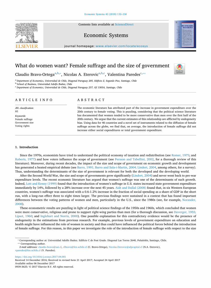
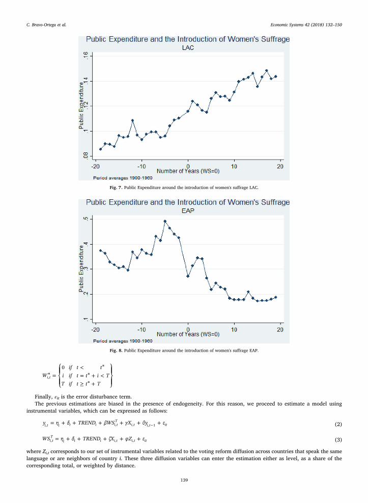
Figs. 5–8 show our event analysis for the whole sample and for the three regions specified. We consider the year in which femalesuffrage was enacted as year 0, and on the x-axis we plot the period between 20 years previous to the reform and the 20 years thatfollowed. On the y-axis, we plot the share of GDP that corresponds to total government expenditure.

These graphs show no clear pattern. While in some regions − ECA and LAC − we observe an upward trend in the share ofgovernment expenditure, in general this trend starts before the reform. Moreover, we also observe one region (EAP) in which there isa clear downward trend that, again, starts before the reform. These trends may be explained in part by other things that werechanging at the time female suffrage was enacted. For example, the EAP decline in government spending after suffrage appears likelyto be caused by the end of WWII, since this region mostly gave women the franchise just after the war. Therefore, we will need toconsider these other factors in order to be able to measure the causal effect of women’s suffrage.

The reported graphs are a clear signal that it is not an easy task to disentangle the real effect women’s suffrage had on governmentsize. There is no consistent pattern, and the changes in trend in government size precede the voting reform in all cases.

6. Econometric framework

To make our results comparable to previous studies, we begin by replicating the methodology presented in Aidt and Dallal (2008).

Fig 4. Diffusion of Women Suffrage in neighboring countries.

Table 1Correlation matrix.

Women’s Suffrage Instrument 2a Instrument 2b

Women’s Suffrage 1.0000Instrument 2a 0.5940*** 1.0000Instrument 2b 0.7409*** 0.7720*** 1.0000Instrument 2c 0.6125*** 0.6950*** 0.6962***

Notes: Instrument 2a is the number of countries that have women’s suffrage, by language. Instrument 2b is the percentage of countries that have women’ssuffrage, by language. Instrument 2c is the number of countries, weighted by distance, that have women’s suffrage, by language.

*** Significant at 1%.


137

That is, we estimate the following regression:

= + + + + + +−y η δ TREND βWS γX θy ε ,i t i t i i tT

i t i t it, , , , 1 (1)

where ηi is the country fixed effect, δt is a time fixed effect, TRENDi is a country time trend variable, yi,t−1 is the lagged endogenousvariable, and Xi, t is a number of control variables, including the country’s divorce rate, the log of single women, female labor forceparticipation, economic franchise, political competition, proportional rule,7 age structure, the log of GDP per capita, education andthe log of population. The dependent variables that we consider in our analysis, yi,t, are total spending as a percentage of GDP, socialspending as a fraction of GDP, and security spending as a fraction of GDP. Finally, we construct the women’s suffrage variable as aspline function, whereWSi takes the value one once the female voting right was enacted, and then increases linearly to T, with T={0,10, 15, 20}. Then, if T = 20 and women’s suffrage was introduced in t= t*,

Fig. 5. Public Expenditure around the introduction of women's suffrage.

Fig 6. Public Expenditure around the introduction of women's suffrage ECA.

7 The proportional rule variable is equal to one if the electoral system is based on proportional representation and equal to zero if it is based on majority rule.


138

=⎧

⎨⎪

⎩⎪

<= + <≥ +

⎫

⎬⎪

⎭⎪W

if t ti if t t i TT if t t T

*0 *

**

i t,

Finally, εit is the error disturbance term.The previous estimations are biased in the presence of endogeneity. For this reason, we proceed to estimate a model using

instrumental variables, which can be expressed as follows:

= + + + + + +−y η δ TREND βWS γX θy εi t i t i i tT

i t i t it, , , , 1 (2)

= + + + + +WS η δ TREND ζX φZ εi tT

i t i i t i t it, , , (3)

where Zi,t corresponds to our set of instrumental variables related to the voting reform diffusion across countries that speak the samelanguage or are neighbors of country i. These three diffusion variables can enter the estimation either as level, as a share of thecorresponding total, or weighted by distance.

Fig. 7. Public Expenditure around the introduction of women's suffrage LAC.

Fig. 8. Public Expenditure around the introduction of women's suffrage EAP.


139

This empirical strategy will provide consistent estimators, given that the variables contained in Zi,t don’t have a direct effect on thecountry’s public expenditure. To test this exclusion restriction, we replace the variable WSi t

T, in Eq. (1) with the average past public

expenditure in neighboring countries. If the exclusion restriction holds, then this variable should have no significant effect on public

Table 3Total government spending as a share of GDP – Aidt’s sample (1860–1960).

OLS IV

(1) (2) (3) (1) (2) (3)

WS, 10 years lag −0.017 −0.075*(0.013) (0.030)

WS, 15 years lag −0.014 −0.058*(0.011) (0.026)

WS, 20 years lag −0.008 −0.052*(0.010) (0.022)

Divorce Rate −0.009 −0.009 −0.008 −0.022 −0.019 −0.018(0.008) (0.008) (0.008) (0.012) (0.010) (0.010)

ln(single women) −0.161 −0.161 −0.174 0.047 0.050 0.004(0.123) (0.124) (0.123) (0.260) (0.264) (0.252)

Female labor force participation −0.901*** −0.894*** −0.906*** −0.625 −0.596 −0.537(0.336) (0.338) (0.342) (0.387) (0.533) (0.591)

Economic franchise −0.001 −0.001 −0.001 −0.002 −0.002 −0.003(0.001) (0.001) (0.001) (0.002) (0.002) (0.002)

Political competition −0.018 −0.018 −0.022 −0.058 −0.067 −0.076(0.042) (0.043) (0.043) (0.063) (0.060) (0.059)

Proportional rule −0.039 −0.040 −0.048 0.042 0.031 0.034(0.045) (0.043) (0.043) (0.074) (0.061) (0.061)

Age structure 0.021 0.019 0.020 0.037 0.029 0.022(0.017) (0.018) (0.018) (0.044) (0.039) (0.037)

ln(gdp per capita) −0.219 −0.199 −0.233 −0.119 −0.077 −0.045(0.142) (0.148) (0.157) (0.302) (0.298) (0.346)

Education −0.239 −0.267 −0.250 −0.633 −0.769* −0.837*(0.197) (0.198) (0.199) (0.388) (0.380) (0.404)

ln(population) −0.417 −0.449 −0.462 0.327 0.218 0.057(0.488) (0.485) (0.485) (1.426) (1.257) (1.140)

Lagged endogenous 0.657*** 0.658*** 0.664*** 0.602*** 0.613*** 0.615***(0.050) (0.049) (0.049) (0.050) (0.050) (0.051)

Observations 409 409 409 351 351 351R-squared 0.966 0.966 0.966 0.581 0.587 0.580Countries 6 6 6 6 6 6Hansen J test 0.821 0.257 0.408F-test, weak Ident 763.300 23.840 10.490

Table 2Effect of past public expenditure in neighboring countries on public expenditure.

VARIABLES OLS

(1) (2) (3)

Lagged average public expenditure in neighboring countries −0.008 0.013 −0.091(0.037) (0.032) (0.058)

Lagged endogenous 0.628*** 0.580*** 0.316***(0.078) (0.049) (0.062)

ln(population) −0.132 0.137 0.137(0.121) (0.160) (0.086)

Age structure 0.000 0.000 0.000*(0.000) (0.000) (0.000)

ln(gdp per capita) 0.068** 0.071*** 0.023(0.029) (0.021) (0.021)

Literacy 0.41 1.590*** −0.115(0.350) (0.579) (0.200)

Political competition 0.005 0.022* 0.001(0.008) (0.012) (0.003)

Observations 745 379 267R-squared 0.852 0.843 0.869Countries 34 13 15

Notes: Model (1) includes all countries in the sample. Model (2) includes countries in ECA and model (3) includes countries in LAC


140

expenditure. Our results, presented in Table 2, show that we cannot reject a zero effect of the past public expenditure in neighboringcountries on public expenditure.

7. Results

We estimate both models for two different samples. First, we use the same data as in Aidt and Dallal (2008). This sample includes6 European countries versus the 46 countries in the second sample. Despite the smaller sample of countries, this sample includesbetter control variables, and we can distinguish between different types of spending. In our second sample, we have more countriesbut a shorter time period and fewer control variables, and we only observe total spending.

7.1. Aidt’s sample

Table 3 replicates the specification used by Aidt and Dallal (2008) but with total government expenditure as a share of GDP as thedependent variable. The first three columns show an OLS set of estimations. We observe that the introduction of women’s suffragedoes not seem to increase total government expenditure at 10, 15 or 20 years after the introduction. As we have discussed, esti-mations by OLS are afflicted by endogeneity bias and therefore, in columns 4 to 6, we estimate the same specifications with in-strumental variables using limited information maximum likelihood (LIML). This new set of estimates shows a negative impact of theintroduction of women’s suffrage after 10, 15 or 20 years. This last set of estimates survives the Hansen’s overidentification and weakinstrument tests. We use Hansen’s tests because these and all the estimations of the paper are computed with robust standard errors.

Regarding other controls, the lagged dependent variable is significant in both OLS and LIML estimations, while female laborparticipation is only significant in the OLS estimates. None of the other controls are significant in any estimation.

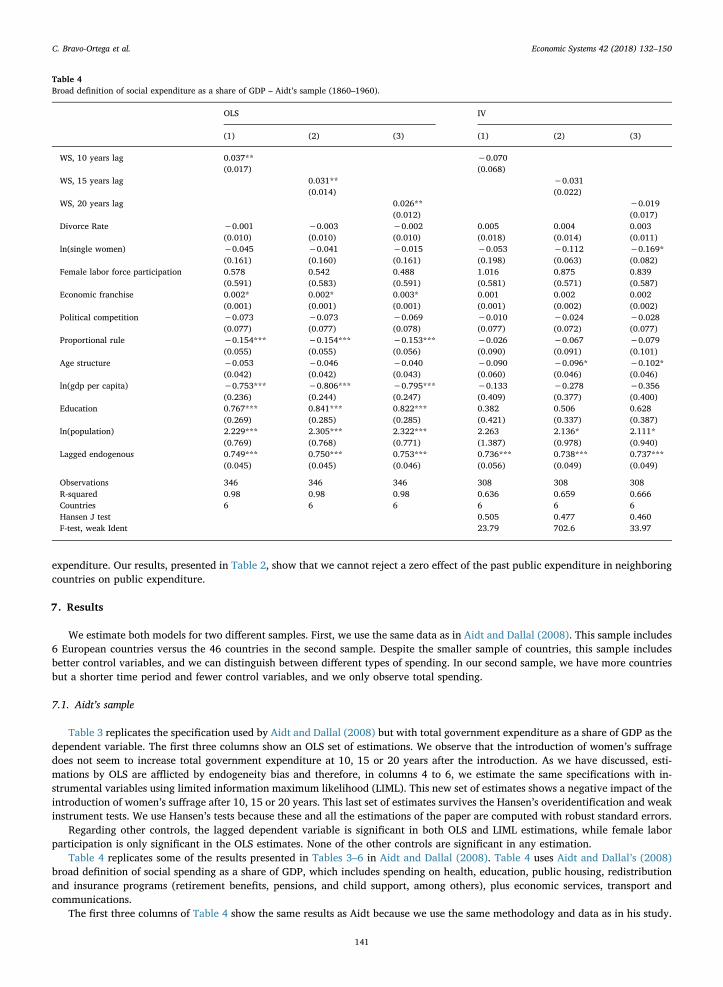
Table 4 replicates some of the results presented in Tables 3–6 in Aidt and Dallal (2008). Table 4 uses Aidt and Dallal’s (2008)broad definition of social spending as a share of GDP, which includes spending on health, education, public housing, redistributionand insurance programs (retirement benefits, pensions, and child support, among others), plus economic services, transport andcommunications.

The first three columns of Table 4 show the same results as Aidt because we use the same methodology and data as in his study.

Table 4Broad definition of social expenditure as a share of GDP – Aidt’s sample (1860–1960).

OLS IV

(1) (2) (3) (1) (2) (3)

WS, 10 years lag 0.037** −0.070(0.017) (0.068)

WS, 15 years lag 0.031** −0.031(0.014) (0.022)

WS, 20 years lag 0.026** −0.019(0.012) (0.017)

Divorce Rate −0.001 −0.003 −0.002 0.005 0.004 0.003(0.010) (0.010) (0.010) (0.018) (0.014) (0.011)

ln(single women) −0.045 −0.041 −0.015 −0.053 −0.112 −0.169*(0.161) (0.160) (0.161) (0.198) (0.063) (0.082)

Female labor force participation 0.578 0.542 0.488 1.016 0.875 0.839(0.591) (0.583) (0.591) (0.581) (0.571) (0.587)

Economic franchise 0.002* 0.002* 0.003* 0.001 0.002 0.002(0.001) (0.001) (0.001) (0.001) (0.002) (0.002)

Political competition −0.073 −0.073 −0.069 −0.010 −0.024 −0.028(0.077) (0.077) (0.078) (0.077) (0.072) (0.077)

Proportional rule −0.154*** −0.154*** −0.153*** −0.026 −0.067 −0.079(0.055) (0.055) (0.056) (0.090) (0.091) (0.101)

Age structure −0.053 −0.046 −0.040 −0.090 −0.096* −0.102*(0.042) (0.042) (0.043) (0.060) (0.046) (0.046)

ln(gdp per capita) −0.753*** −0.806*** −0.795*** −0.133 −0.278 −0.356(0.236) (0.244) (0.247) (0.409) (0.377) (0.400)

Education 0.767*** 0.841*** 0.822*** 0.382 0.506 0.628(0.269) (0.285) (0.285) (0.421) (0.337) (0.387)

ln(population) 2.229*** 2.305*** 2.322*** 2.263 2.136* 2.111*(0.769) (0.768) (0.771) (1.387) (0.978) (0.940)


Observations 346 346 346 308 308 308R-squared 0.98 0.98 0.98 0.636 0.659 0.666Countries 6 6 6 6 6 6Hansen J test 0.505 0.477 0.460F-test, weak Ident 23.79 702.6 33.97


141

We observe that the OLS estimates indeed show a positive effect of women’s suffrage on the broad definition of social spending 10, 15and 20 years after the introduction. However, when we estimate the model using instrumental variables, this positive effect becomesinsignificant. Again, all LIML estimations survive the Hansen’s and weak instruments tests and show robust standard errors.

Regarding other controls, the lagged dependent variable and population are positive and significant in both OLS and LIMLestimations, while economic franchise and education are only significant in the OLS estimates and show positive coefficients. GDP percapita and proportional rule are also significant in the OLS estimates, but show negative signs. None of the other controls aresignificant in any estimation.

We investigate whether female voting has had an impact on other types of public spending such as defense, and find that it doesnot. In this case, none of the OLS and LIML coefficients linked to the introduction of women’s suffrage turn out to be significant. AllLIML estimations survive the specifications tests.

Regarding other controls, the lagged dependent variable is positive and significant in both the OLS and the LIML estimations,while education and GDP per capita show a negative and significant coefficient in some of the estimations. None of the other controlsare significant in any of the estimations.

7.2. Whole sample

We replicate our estimations for the second database, which includes 46 countries. It should be noted that the time period isshorter as it covers only the period 1900–1960, and we have fewer control variables.

In Table 6, as a first exercise, we run a restricted sample that includes the six countries from Aidt and Dallal’s (2008) sample. Weagain see a marginally positive effect of women’s suffrage when using OLS, which is significant even ten years after the introductionof women’s suffrage. However, this positive effect disappears when using instrumental variables. All LIML estimations survive theHansen’s and weak instruments tests by a wide margin.

Regarding other controls, the lagged dependent variable is positive and significant and age structure is negative and significant inboth the OLS and the LIML estimations, while literacy, political competition and GDP per capita show a positive and significantcoefficient in the OLS estimations. Population does not show as significant in any estimation.

Because the inclusion of both the lagged endogenous variable and the country-specific trend control may lead to us finding no

Table 5Spending on defense as a share of GDP – Aidt’s sample (1860–1960).

OLS IV

(1) (2) (3) (1) (2) (3)

WS, 10 years lag 0.012 −0.061(0.021) (0.031)

WS, 15 years lag 0.016 −0.041(0.017) (0.038)

WS, 20 years lag 0.018 −0.032(0.016) (0.032)

Divorce Rate 0.006 0.005 0.004 0.011 0.012 0.010(0.013) (0.013) (0.013) (0.014) (0.017) (0.015)

ln(single women) −0.307 −0.310 −0.301 −0.151 −0.152 −0.205(0.196) (0.198) (0.198) (0.335) (0.289) (0.227)

Female labor force participation −0.613 −0.651 −0.715 −0.224 −0.236 −0.216(0.678) (0.670) (0.677) (0.392) (0.435) (0.416)

Economic franchise 0.000 0.000 0.000 −0.001 −0.001 −0.001(0.002) (0.002) (0.002) (0.002) (0.002) (0.002)

Political competition 0.035 0.032 0.032 0.054 0.044 0.041(0.094) (0.095) (0.095) (0.088) (0.076) (0.069)

Proportional rule 0.000 −0.008 −0.017 0.090 0.072 0.068(0.066) (0.065) (0.066) (0.060) (0.076) (0.079)

Age structure −0.027 −0.023 −0.018 −0.023 −0.026 −0.035(0.053) (0.053) (0.054) (0.064) (0.051) (0.041)

ln(gdp per capita) −0.494 −0.568* −0.621* −0.031 −0.025 −0.065(0.315) (0.334) (0.352) (0.688) (0.782) (0.737)

Education −0.395 −0.324 −0.290 −0.850** −0.917 −0.824(0.327) (0.338) (0.336) (0.323) (0.526) (0.508)

ln(population) 0.750 0.787 0.814 0.817 0.733 0.697(0.895) (0.905) (0.911) (0.420) (0.406) (0.479)


Observations 337 337 337 299 299 299R-squared 0.957 0.957 0.958 0.705 0.706 0.706Countries 6 6 6 6 6 6Hansen J test 0.937 0.963 0.846F-test, weak Ident 68.2 2233 19.55


142

Table6

Totalgo

vernmen

tspen

ding

asashareof

GDP–Cou

ntries

includ

edin

Aidt’s

sample(190

0–19

60).

OLS

IVIV

VARIA

BLES

(1)

(2)

(3)

(4)

(5)

(6)

(7)

(8)

(9)

(10)

(11)

(12)

WS

0.00

30.01

0−

0.02

6*(0.009

)(0.016

)(0.010

)WS,

10ye

arslag

0.00

2*0.00

1−0.00

4(0.001

)(0.003

)(0.002

)WS,

15ye

arslag

0.00

20.00

0−0.00

4(0.001

)(0.002

)(0.002

)WS,

20ye

arslag

0.00

10.00

0−0.00

4*(0.001

)(0.002

)(0.002

)Po

litical

compe

tition

0.02

8***

0.02

9***

0.03

0***

0.03

0***

0.02

70.02

90.02

90.02

90.02

90.02

90.02

80.02

6(0.009

)(0.009

)(0.009

)(0.009

)(0.015

)(0.015

)(0.016

)(0.016

)(0.016

)(0.018

)(0.019

)(0.020

)Age

structure

−0.00

0**

−0.00

0***

−0.00

0***

−0.00

0**

−0.00

0*−

0.00

0*−

0.00

0**

−0.00

0**

0.00

0*0.00

00.00

00.00

00.00

00.00

00.00

00.00

00.00

00.00

00.00

00.00

00.00

00.00

00.00

00.00

0ln(gdp

percapita)

0.06

3**

0.05

2*0.05

2*0.05

6*0.06

10.05

70.06

10.06

40.06

1**

0.07

6**

0.07

7*0.07

6*(0.026

)(0.027

)(0.029

)(0.031

)(0.033

)(0.041

)(0.047

)(0.050

)(0.018

)(0.029

)(0.031

)(0.032

)Literates

1.57

6***

1.97

0***

1.99

0***

1.78

8**

1.71

0*1.80

41.62

61.52

90.19

50.09

3−0.03

0−0.21

7(0.590

)(0.678

)(0.706

)(0.696

)(0.809

)(1.069

)(1.271

)(1.266

)(0.306

)(0.273

)(0.194

)(0.130

)ln(pop

ulation)

0.10

30.10

10.11

50.12

00.10

00.10

20.10

70.10

6−

0.07

1−0.05

9−0.05

3−0.05

3(0.161

)(0.160

)(0.164

)(0.171

)(0.168

)(0.154

)(0.174

)(0.198

)(0.071

)(0.089

)(0.093

)(0.088

)La

gged

endo

geno

us0.60

4***

0.60

6***

0.60

0***

0.60

1***

0.60

9***

0.60

5***

0.60

1***

0.60

2***

0.62

3***

0.62

5***

0.63

4***

0.63

4***

(0.049

)(0.048

)(0.048

)(0.048

)(0.045

)(0.039

)(0.040

)(0.040

)(0.019

)(0.028

)(0.023

)(0.022

)

Observa

tion

s33

433

433

433

433

433

433

433

433

433

433

433

4R-squ

ared

0.92

90.92

90.92

90.92

90.64

60.65

0.64

80.64

70.62

10.61

10.61

40.61

5Cou

ntries

66

66

66

66

66

66

Jointsign

ificanc

eof

coun

tryspecifictren

ds(Prob>

F)0.01

00.00

50.00

50.00

40.00

60.00

00.00

00.00

0F-test,w

eakIden

t23

3.60

5.83

101.40

162.90

2006

.00

41.32

96.32

285.50

Han

senJtest

0.70

70.94

00.89

00.80

20.24

80.42

40.50

60.42

0Cou

ntry

fixedeff

ect

yes

yes

yes

yes

yes

yes

yes

yes

yes

yes

yes

yes

Yearfixedeff

ect

yes

yes

yes

yes

yes

yes

yes

yes

yes

yes

yes

yes

Cou

ntry

specifictimetren

dye

sye

sye

sye

sye

sye

sye

sye

sno

nono

no

Notes:S

tand

arderrors,c

lustered

attheco

untryleve

l,arepresen

tedin

parenthe

ses.

***p

<0.01

.**

p<

0.05

.*p

<0.1.


143

effect, we repeat our instrumental variable regressions without the time trends. Our results show a negative effect on public spendingimmediately after the introduction of women’s suffrage. When we test the joint significance of the country-specific trends we cannotrule out that they are needed; however, the point estimates of the time trends turn out to be not significant. These two results aretypically reported when there is multicollinearity. Furthermore, considering that there are two other variables that also move to-gether with the trend (population and GDP), we consider that we can safely rule out estimations without the trends. The samesituation occurs again in the following tables with regional samples.

The estimations in Table 7 include all 46 countries. Both OLS and LIML estimations show no effect of women’s suffrage on totalgovernment expenditure. The LIML estimates survive the Hansen’s overidentification and the weak instrument tests, except for thelast specification, where the test is between the critical values associated with the 10% and 15% maximal LIML size. Regarding othercontrols, the lagged dependent variable, literacy and GDP per capita are positive and significant in almost all OLS and LIML esti-mations. No other variable is significant in any estimation.

Table 8 reports the estimations for Europe and Central Asia. In this case, both OLS and LIML estimates show no effect of theintroduction of women’s suffrage. In this case, the estimated coefficients are not only not significant, but also have point estimatesthat are very close to zero. The LIML estimates survive the Hansen’s overidentification and the weak instrument tests, except for thesecond specification. Regarding other controls, the lagged dependent variable, GDP per capita and literacy are positive and sig-nificant in both OLS and LIML estimations, while political competition shows a positive and significant coefficient in the OLS esti-mations and age structure shows a negative sign in the OLS as well. Population is not significant in any estimation.

Table 9 shows the estimations for Latin America and the Caribbean. In this case, we find a positive and statistically significant

Table 7Total government spending as a share of GDP – Whole sample (1900–1960).

OLS IV IV

VARIABLES (1) (2) (3) (4) (5) (6) (7) (8) (9) (10) (11) (12)

WS −0.006 0.000 0.022(0.004) (0.011) (0.016)

WS, 10 years lag −0.001 0.000 0.002(0.001) (0.001) (0.002)

WS, 15 years lag −0.001 0.001 0.002(0.001) (0.001) (0.001)

WS, 20 years lag −0.001 0.001 0.0020.000 (0.001) (0.001)

Politicalcompetition

0.005 0.004 0.004 0.005 0.004 0.003 0.003 0.002 −0.006 −0.005 −0.005 −0.005

(0.004) (0.004) (0.004) (0.004) (0.004) (0.003) (0.003) (0.003) (0.006) (0.006) (0.006) (0.007)Age structure −0.000* 0.000 0.000 0.000 0.000 0.000 0.000 0.000 0.000 0.000 0.000 0.000

0.000 0.000 0.000 0.000 0.000 0.000 0.000 0.000 0.000 0.000 0.000 0.000ln(gdp per

capita)0.053*** 0.054*** 0.054*** 0.055*** 0.054*** 0.054*** 0.053*** 0.052*** 0.046*** 0.042*** 0.040*** 0.039***

(0.012) (0.012) (0.012) (0.011) (0.015) (0.014) (0.014) (0.014) (0.012) (0.011) (0.011) (0.011)Literates 0.184** 0.185** 0.184** 0.185** 0.198 0.202 0.212* 0.218* 0.038 0.052 0.063 0.073

(0.075) (0.080) (0.081) (0.079) (0.120) (0.121) (0.125) (0.129) (0.031) (0.036) (0.042) (0.048)ln(population) −0.052 −0.055 −0.054 −0.055 −0.065 −0.068 −0.076 −0.080 −0.054** −0.049** −0.047** −0.045**

(0.051) (0.056) (0.055) (0.052) (0.060) (0.058) (0.055) (0.051) (0.023) (0.021) (0.021) (0.021)War 0.040*** 0.041*** 0.041*** 0.041*** 0.040*** 0.040*** 0.040*** 0.040*** 0.042*** 0.042*** 0.041*** 0.041***

(0.006) (0.006) (0.006) (0.006) (0.010) (0.010) (0.010) (0.010) (0.009) (0.009) (0.009) (0.009)Lagged

endogenous0.707*** 0.707*** 0.707*** 0.707*** 0.708*** 0.709*** 0.709*** 0.710*** 0.765*** 0.766*** 0.766*** 0.765***

(0.029) (0.029) (0.029) (0.029) (0.032) (0.032) (0.032) (0.032) (0.029) (0.030) (0.030) (0.031)

Observations 1323 1323 1323 1323 1320 1320 1320 1320 1320 1320 1320 1320R-squared 0.893 0.893 0.893 0.893 0.714 0.714 0.713 0.712 0.69 0.692 0.691 0.69Countries 46 46 46 46 43 43 43 43 43 43 43 43Joint significance

of countryspecifictrends(Prob>F)

0.000 0.000 0.000 0.000 0.000 0.000 0.000 0.000

F-test, weakIdent

5.78 6.78 4.88 3.93 3.92 7.92 5.57 3.73

Hansen J test 0.364 0.378 0.409 0.434 0.209 0.328 0.303 0.281Country fixed

effectyes yes yes yes yes yes yes yes yes yes yes yes

Year fixed effect yes yes yes yes yes yes yes yes yes yes yes yesCountry specific

time trendyes yes yes yes yes yes yes yes no no no no

Notes: Standard errors, clustered at the country level, are presented in parentheses. *** p < 0.01, ** p < 0.05, * p < 0.1.


144

Table8

Totalgo

vernmen

tspen

ding

asashareof

GDP−

Europe

andCen

tral

Asia(190

0–19

60).

OLS

IVIV

VARIA

BLES

(1)

(2)

(3)

(4)

(5)

(6)

(7)

(8)

(9)

(10)

(11)

(12)

WS

−0.00

60.01

40.01

3(0.005

)(0.021

)(0.015

)WS,

10ye

arslag

0.00

00.00

10.00

0(0.001

)(0.003

)(0.002

)WS,

15ye

arslag

0.00

00.00

00.00

0(0.001

)(0.003

)(0.001

)WS,

20ye

arslag

−0.00

10.00

00.00

0(0.001

)(0.003

)(0.001

)Po

litical

compe

tition

0.01

8**

0.01

6**

0.01

6**

0.01

6**

0.01

00.01

40.01

50.01

5−

0.00

5−0.00

2−0.00

2−0.00

2(0.007

)(0.007

)(0.007

)(0.007

)(0.012

)(0.009

)(0.009

)(0.009

)(0.013

)(0.012

)(0.011

)(0.011

)Age

structure

−0.00

0***

−0.00

0***

−0.00

0***

−0.00

0***

0.00

00.00

00.00

00.00

00.00

00.00

00.00

00.00

00.00

00.00

00.00

00.00

00.00

00.00

00.00

00.00

00.00

00.00

00.00

00.00

0ln(gdp

percapita)

0.10

5***

0.10

4***

0.10

5***

0.10

7***

0.09

9***

0.10

1***

0.10

3***

0.10

4**

0.06

0***

0.06

1***

0.06

1***

0.06

0***

(0.015

)(0.015

)(0.015

)(0.015

)(0.032

)(0.029

)(0.032

)(0.036

)(0.018

)(0.018

)(0.019

)(0.019

)Literates

0.61

3***

0.60

8***

0.60

7***

0.60

5***

0.59

2**

0.60

3**

0.60

6**

0.60

6**

0.00

40.01

40.01

10.01

2(0.173

)(0.173

)(0.171

)(0.170

)(0.268

)(0.241

)(0.232

)(0.227

)(0.027

)(0.038

)(0.040

)(0.040

)ln(pop

ulation)

−0.11

7−0.12

3−

0.11

9−0.11

9−0.15

1−0.13

8−0.12

8−

0.12

6−

0.11

5*−0.10

1−0.09

6−0.10

0(0.078

)(0.081

)(0.080

)(0.078

)(0.136

)(0.135

)(0.148

)(0.146

)(0.053

)(0.063

)(0.068

)(0.072

)War

0.04

0***

0.04

0***

0.04

0***

0.04

0***

0.04

0**

0.04

0**

0.04

0**

0.04

0**

0.03

9**

0.04

0**

0.04

0**

0.04

0**

(0.005

)(0.005

)(0.005

)(0.005

)(0.018

)(0.018

)(0.018

)(0.018

)(0.017

)(0.017

)(0.017

)(0.017

)La

gged

endo

geno

us0.63

8***

0.64

1***

0.64

1***

0.64

0***

0.64

9***

0.64

3***

0.64

2***

0.64

1***

0.71

0***

0.70

3***

0.70

3***

0.70

4***

(0.025

)(0.024

)(0.024

)(0.024

)(0.055

)(0.053

)(0.053

)(0.053

)(0.039

)(0.040

)(0.040

)(0.039

)

Observa

tion

s59

759

759

759

759

759

759

759

759

759

759

759

7R-squ

ared

0.87

40.87

40.87

40.87

40.67

0.67

30.67

40.67

40.65

30.65

60.65

60.65

6Cou

ntries

1414

1414

1414

1414

1414

1414

Jointsign

ificanc

eof

coun

tryspecifictren

ds(Prob>

F)0.00

00.00

00.00

00.00

00.00

00.00

00.00

00.00

0F-test,w

eakIden

t1.88

5.63

3.98

4.87

1.86

5.44

10.89

37.56

Han

senJtest

0.54

00.59

90.59

30.58

10.33

90.34

20.33

60.34

3Cou

ntry

fixedeff

ect

yes

yes

yes

yes

yes

yes

yes

yes

yes

yes

yes

yes

Yearfixedeff

ect

yes

yes

yes

yes

yes

yes

yes

yes

yes

yes

yes

yes

Cou

ntry

specifictimetren

dye

sye

sye

sye

sye

sye

sye

sye

sno

nono

no

Notes:S

tand

arderrors,c

lustered

attheco

untryleve

l,arepresen

tedin

parenthe

ses.

***p

<0.01

,**

p<

0.05

,*p

<0.1.


145

Table9

Totalgo

vernmen

tspen

ding

asashareof

GDP–La

tinAmericaan

dtheCaribbe

an(190

0–19

60).

OLS

IVIV

VARIA

BLES

(1)

(2)

(3)

(4)

(5)

(6)

(7)

(8)

(9)

(10)

(11)

(12)

WS

0.00

3−0.00

3−0.00

9(0.003

)(0.008

)(0.007

)WS,

10ye

arslag

−0.00

2***

0.00

00.00

20.00

0(0.001

)(0.002

)WS,

15ye

arslag

−0.00

1***

0.00

10.00

30.00

0(0.002

)(0.002

)WS,

20ye

arslag

−0.00

1***

0.00

30.00

2*0.00

0(0.003

)(0.001

)Po

litical

compe

tition

−0.00

2−0.00

3−0.00

2−0.00

2−0.00

2−

0.00

2−0.00

2−

0.00

2−0.00

2−

0.00

5**

−0.00

9*−0.00

6*(0.003

)(0.002

)(0.002

)(0.002

)(0.004

)(0.004

)(0.004

)(0.004

)(0.003

)(0.002

)(0.004

)(0.003

)Age

structure

0.00

0−0.00

0*0.00

00.00

00.00

00.00

00.00

00.00

00.00

00.00

00.00

00.00

00.00

00.00

00.00

00.00

00.00

00.00

00.00

00.00

00.00

00.00

00.00

00.00

0ln(gdp

percapita)

0.00

70.00

80.00

70.00

70.00

80.00

70.00

80.00

90.00

90.00

4−

0.00

30.00

2(0.006

)(0.007

)(0.006

)(0.006

)(0.009

)(0.009

)(0.011

)(0.014

)(0.013

)(0.011

)(0.015

)(0.013

)Literates

0.10

40.13

50.11

60.12

00.11

90.11

60.10

70.09

20.07

80.09

10.11

50.10

8(0.105

)(0.104

)(0.102

)(0.101

)(0.075

)(0.086

)(0.075

)(0.066

)(0.072

)(0.097

)(0.118

)(0.098

)ln(pop

ulation)

−0.00

3−0.01

6−0.01

3−0.01

9−0.00

8−

0.00

80.00

10.02

4−0.03

3−

0.04

6−

0.04

7−0.04

1(0.034

)(0.034

)(0.033

)(0.034

)(0.023

)(0.025

)(0.025

)(0.038

)(0.026

)(0.039

)(0.046

)(0.030

)War

0.00

20.00

10.00

20.00

10.00

10.00

10.00

10.00

2−0.00

3−

0.00

4−

0.00

7−0.00

4(0.003

)(0.003

)(0.003

)(0.002

)(0.002

)(0.003

)(0.005

)(0.005

)(0.004

)(0.006

)(0.010

)(0.005

)La

gged

endo

geno

us0.44

1***

0.42

8***

0.43

8***

0.43

8***

0.44

9***

0.44

1***

0.45

0***

0.45

9***

0.66

8***

0.69

3***

0.71

5***

0.69

3***

(0.039

)(0.037

)(0.038

)(0.038

)(0.062

)(0.062

)(0.059

)(0.062

)(0.072

)(0.084

)(0.085

)(0.075

)

Observa

tion

s40

540

540

540

540

540

540

540

540

540

540

540

5R-squ

ared

0.89

80.90

10.89

90.89

90.62

60.63

10.62

10.59

80.54

40.50

20.45

10.51

9Cou

ntries

1717

1717

1717

1717

1717

1717

Jointsign

ificanc

eof

coun

tryspeci fictren

ds(Prob>

F)0.00

00.00

00.00

00.00

00.00

00.00

00.00

00.00

0F-test,w

eakIden

t8.67

15.91

5.32

1.78

11.15

1.04

0.96

2.01

Han

senJtest

0.51

20.52

10.52

20.37

80.15

20.09

90.21

80.14

9Cou

ntry

fixedeff

ect

yes

yes

yes

yes

yes

yes

yes

yes

yes

yes

yes

yes

Yearfixedeff

ect

yes

yes

yes

yes

yes

yes

yes

yes

yes

yes

yes

yes

Cou

ntry

specifictimetren

dye

sye

sye

sye

sye

sye

sye

sye

sno

nono

no

Notes:S

tand

arderrors,c

lustered

attheco

untryleve

l,arepresen

tedin

parenthe

ses.

***p

<0.01

,**

p<

0.05

,*p

<0.1.


146

effect when using OLS. As with the countries included in Aidt’s sample, this effect disappears when using instrumental variables. TheLIML estimates survive the Hansen’s overidentification and the weak instrument tests, except in the last specification. Regardingother controls, the only significant variable is the lagged dependent variable in both OLS and LIML estimations. No other variables aresignificant in any estimation. There is, however, a minor change in the impact of the introduction of female voting after 20 years thatturns out to be significant and positive once time trends are omitted.8

Finally, Table 10 shows the estimations for the East Asia and the Pacific sample. In this case, although we find no effect ofwomen’s suffrage on total government expenditure when using OLS, a positive and significant effect appears when using instrumentalvariables. The LIML estimates survive the Hansen’s overidentification test and the weak instrument tests by a wide margin.

Regarding other controls, the lagged dependent variable coefficient is positive and significant in both OLS and LIML estimations,while the coefficient for age structure is negative and significant in the LIML estimations. The coefficient for literacy is positive andsignificant in the same set of estimations. No other variable is significant in any estimation.

Table 10 ws estimations that do not include time trend variables, indicating that there is no effect or a small negative effect of theintroduction of female voting after 20 years. As we discussed, our preferred estimations do not consider time trends, as there is strongevidence of multicollinearity, and the point estimates of the trend variables are not significant.

8. Concluding remarks

In this paper, we investigate the effect of the introduction of female suffrage on the size of government. For this purpose, we

Table 10Total government spending as a share of GDP– East Asia and the Pacific (1900–1960).

OLS IV IV

VARIABLES (1) (2) (3) (4) (5) (6) (7) (8) (9) (10) (11) (12)

WS −0.072 0.109** 0.000(0.089) (0.031) (0.014)

WS, 10 years lag −0.001 0.020** −0.007(0.018) (0.007) (0.005)

WS, 15 years lag 0.014 0.023** −0.006(0.017) (0.007) (0.005)

WS, 20 years lag 0.010 0.020* −0.003*(0.014) (0.008) (0.001)

Politicalcompetition

Age structure 0.000 0.000 0.000 0.000 −0.000*** −0.000** −0.000** −0.000** −0.000*** 0.000 0.000 0.0000.000 0.000 0.000 0.000 0.000 0.000 0.000 0.000 0.000 0.000 0.000 0.000

ln(gdp per capita) 0.023 0.046 0.008 0.019 0.074*** 0.004 −0.016 −0.004 0.067** 0.076** 0.083** 0.079**(0.085) (0.090) (0.098) (0.093) (0.008) (0.023) (0.025) (0.029) (0.016) (0.021) (0.023) (0.018)

Literates 1.526 1.908 2.759 2.591 2.674* 3.073* 3.274* 3.183* 0.156** 0.104 0.086 0.149**(1.526) (1.767) (1.727) (1.757) (0.971) (1.208) (1.211) (1.234) (0.038) (0.064) (0.073) (0.044)

ln(population) −0.397 −0.705 −0.991 −0.920 −1.260* −1.256 −1.158 −1.096 −0.018 0.020 0.024 0.032(0.908) (0.957) (0.935) (0.934) (0.533) (0.654) (0.589) (0.563) (0.049) (0.035) (0.043) (0.072)

War 0.004 0.007 0.007 0.007 0.012 0.011 0.007 0.007 0.009 0.007 0.008 0.008(0.020) (0.021) (0.023) (0.022) (0.006) (0.006) (0.006) (0.005) (0.008) (0.007) (0.008) (0.008)

Laggedendogenous

0.488** 0.520** 0.520** 0.503** 0.573*** 0.551*** 0.519*** 0.486** 0.684*** 0.644*** 0.652*** 0.660***

(0.202) (0.209) (0.222) (0.224) (0.093) (0.076) (0.089) (0.115) (0.074) (0.088) (0.078) (0.057)

Observations 160 160 160 160 159 159 159 159 159 159 159 159R-squared 0.96 0.959 0.96 0.96 0.654 0.69 0.719 0.715 0.686 0.694 0.684 0.687Countries 6 6 6 6 5 5 5 5 5 5 5 5Joint significance

of countryspecific trends(Prob>F)

0.306 0.730 0.412 0.054 0.001 0.000 0.000 0.000

F-test, weak Ident 138.70 22.62 212.40 180.30 33.93 29.94 26.31 33.06Hansen J test 0.128 0.230 0.169 0.319 0.197 0.234 0.248 0.241Country fixed

effectyes yes yes yes yes yes yes yes yes yes yes yes

Year fixed effect yes yes yes yes yes yes yes yes yes yes yes yesCountry specific

time trendyes yes yes yes yes yes yes yes no no no no

Notes: Standard errors, clustered at the country level, are presented in parentheses. *** p < 0.01, ** p < 0.05, * p < 0.1.

8 See the discussion in the previous paragraph regarding the inclusion of time trend variables.


147

carefully address the endogeneity that confounds the relationship between these two variables using a sample of 46 countries withdata covering the first half of the 20th century.

In our estimations, we use as instruments variables related to the voting reform diffusion across countries that speak the samelanguage or that are neighbors. In most of our estimations, these instruments passed the weak instrument and overidentification tests,thus giving credence to our results. Moreover, our instrumental variables estimations challenge the results from OLS estimations fortwo regional subsamples and Aidt’s restricted sample estimations. These results highlight the relevance of properly addressing en-dogeneity when studying the impact of the introduction of female voting on fiscal expenditure.

Contrary to the existing consensus, our main findings show that the introduction of female suffrage has no impact on the size ofgovernment, with the exception of the East Asian Pacific countries, where in one set of estimations we find a positive effect and noeffect in another set. Thus, there is no evidence that a “modern gender gap” regarding public expenditure preferences has influencedthe size and scope of government, at least in Europe and Latin America, which include 31 countries in total.

Despite our “no results,” we can extract some lessons regarding the external and internal validity of papers such as ours. Studieswith many countries have limited external validity; indeed, the behavior of women has evolved significantly across countries and,most importantly, over time within countries.

Very importantly, we consider that, before drawing lessons from an empirical study, it is important to look at the historicalfoundations of the phenomena under scrutiny, which can bring either a reasonable quota of skepticism or wider support to the results.

From a public policy point of view or when analyzing electoral platforms, there must be a recognition that women’s preferencesmight show important differences across countries and even within a country over time. Moreover, understanding differences inpreferences between women and men is a complex matter that goes well beyond economics reasoning; disciplines such as sociology,anthropology and even neuroscience can contribute to this understanding.

In future research, we will address the impact of female political participation on parliaments, and whether this participation haschanged the government budgeting process along the lines of the “modern gender gap” for the period 1960–2010.

Acknowledgements

We thank seminar participants at the Center of Microdata-Nucleo Milenio at the Universidad de Chile and graduate seminarparticipants at the University of Essex for their comments. We also thank Toke Aidt for sharing relevant data with us. The authorsacknowledge Fondecyt Grant1130575, which helped to fund this research. Valentina Paredes acknowledge funding from the Centrefor Social Conflict and Cohesion Studies[CONICYT/FONDAP/15130009].

Appendix A

Table A1Year of introduction of women's suffrage.

Country Region Language Women’s Suffrage Country Region Language Women’s Suffrage

Argentina LAC Spanish 1947 Mexico LAC Spanish 1947Austria ECA German 1919 Morocco MENA Arabic 1963Belgium ECA Dutch 1919 Netherlands ECA Dutch 1920Brazil LAC Portuguese 1932 New Zealand EAP English 1893Canada Na English 1917 Nicaragua LAC Spanish 1955Chile LAC Spanish 1949 Norway ECA Norwegian 1913Colombia LAC Spanish 1954 Pakistan SA Urdu 1947Costa Rica LAC Spanish 1949 Panama LAC Spanish 1946Denmark ECA Danish 1916 Paraguay LAC Spanish 1961Dominican Republic LAC Spanish 1942 Peru LAC Spanish 1955Ecuador LAC Spanish 1967 Philippines EAP English 1937Egipt MENA Arabic 1956 Portugal ECA Portuguese 1975El Salvador LAC Spanish 1939 South Korea EAP Korean 1948Finland ECA Swedish 1906 Spain ECA Spanish 1931France ECA French 1945 Sri Lanka SA Sinhala 1931Ghana SAA English 1954 Sweden ECA Swedish 1921Greece ECA Greek 1952 Switzerland ECA German 1971Guatemala LAC Spanish 1946 Thailand EAP Thai 1932Honduras LAC Spanish 1955 Turkey ECA Turkish 1930Iran MENA Persian 1963 United Kingdom ECA English 1929Iraq MENA Arabic 1980 United States NA English 1920Italy ECA Italian 1945 Uruguay LAC Spanish 1932Japan EAP Japanese 1947 Venezuela LAC Spanish 1946

Notes: Countries are classified within these regions according to the World Bank geographical classification. Women’s suffrage refers to the year the legislation thatenfranchised women was introduced.


148

References

Acemoglu, Daron, Robinson, James A., 2000. Why did the west extend the franchise? democracy, inequality, and growth in historical perspective. Q. J. Econ. 115,1167–1199.

Aidt, Toke S., Dallal, Bianca, 2008. Female voting power: the contribution of women’s suffrage to the growth of social spending in western europe (1869–1960). PublicChoice 134 (3–4), 391–417.

Aidt, Toke S., Eterovic, Dalibor S., 2011. Political competition, electoral participation and public finance in 20th century Latin America. Eur. J. Political Econ. 27 (1),181–200.

Aidt, Toke. S., Jensen, P.S., 2014. Workers of the world unite! franchise extensions and the threat of revolution in europe, 1820–1938. Eur. Econ. Rev. 72, 52–75.Aidt, Toke. S., Dutta, Jayasri, Loukoianova, Elena, 2006. Democracy comes to europe: franchise extension and fiscal outcomes 1830–1938. Eur. Econ. Rev. 50 (2),

249–283.Barro, Robert J., Sala-i-Martin, Xavier, 2004. Economic Growth. MIT Press, Cambridge, Massachusettes.Barro, Robert J., 1991. Economic growth in a cross section of countries. Q. J. Econ. 106 (2), 407.Baxter, Sandra, Lansing, Marjorie, 1983. Women and Politics: The Visible Majority. University of Michigan Press.Cavalcanti, Tiago, V de, V., Tavares, José, 2011. Women prefer larger governments: growth, structural transformation, and government size. Econ. Inq. 49 (1),

155–171.Chattopadhyay, Raghabendra, Duflo, Esther, 2004. Women as policy makers: evidence from a randomized policy experiment in India. Econometrica 72 (5),

1409–1443.Dow, Malcolm M., Burton, Michael L., White, Douglas R., Reitz, Karl P., 1984. Galton’s problem as network autocorrelation. Am. Ethnol. 11, 754–770.Duverger, Maurice, 1955. The Political Role of Women. UNESCO, Paris.

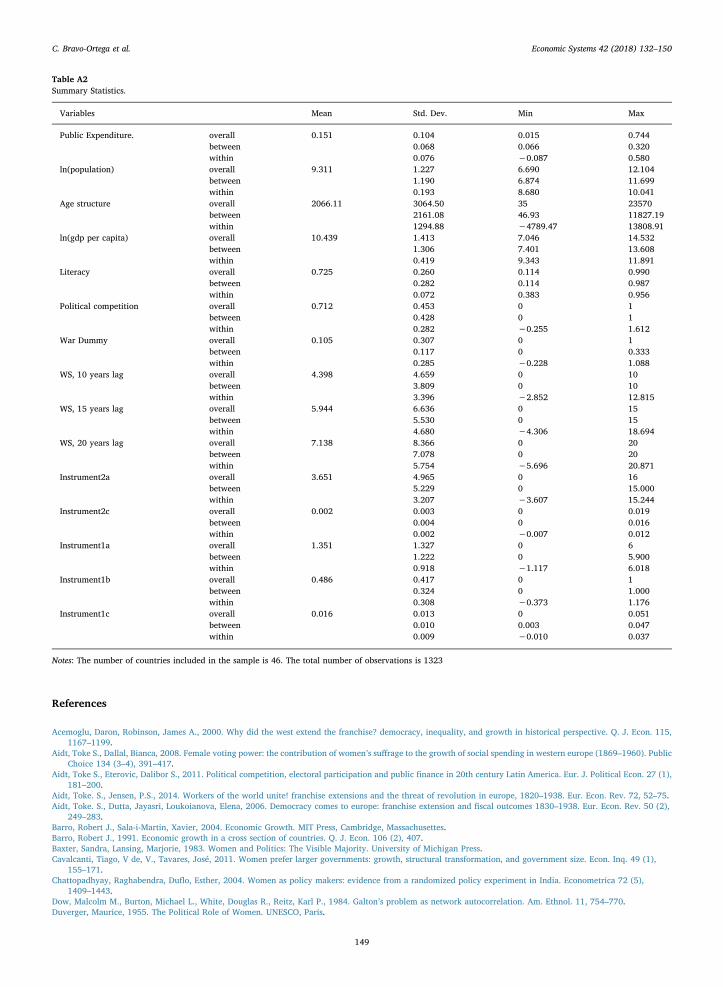
Table A2Summary Statistics.

Variables Mean Std. Dev. Min Max

Public Expenditure. overall 0.151 0.104 0.015 0.744between 0.068 0.066 0.320within 0.076 −0.087 0.580

ln(population) overall 9.311 1.227 6.690 12.104between 1.190 6.874 11.699within 0.193 8.680 10.041

Age structure overall 2066.11 3064.50 35 23570between 2161.08 46.93 11827.19within 1294.88 −4789.47 13808.91

ln(gdp per capita) overall 10.439 1.413 7.046 14.532between 1.306 7.401 13.608within 0.419 9.343 11.891

Literacy overall 0.725 0.260 0.114 0.990between 0.282 0.114 0.987within 0.072 0.383 0.956

Political competition overall 0.712 0.453 0 1between 0.428 0 1within 0.282 −0.255 1.612

War Dummy overall 0.105 0.307 0 1between 0.117 0 0.333within 0.285 −0.228 1.088

WS, 10 years lag overall 4.398 4.659 0 10between 3.809 0 10within 3.396 −2.852 12.815



Instrument2a overall 3.651 4.965 0 16between 5.229 0 15.000within 3.207 −3.607 15.244

Instrument2c overall 0.002 0.003 0 0.019between 0.004 0 0.016within 0.002 −0.007 0.012

Instrument1a overall 1.351 1.327 0 6between 1.222 0 5.900within 0.918 −1.117 6.018

Instrument1b overall 0.486 0.417 0 1between 0.324 0 1.000within 0.308 −0.373 1.176

Instrument1c overall 0.016 0.013 0 0.051between 0.010 0.003 0.047within 0.009 −0.010 0.037

Notes: The number of countries included in the sample is 46. The total number of observations is 1323


149

http://refhub.elsevier.com/S0939-3625(17)30094-8/sbref0005


















Elkins, Zachary, Simmons, Beth, 2005. On waves, clusters, and diffusion: a conceptual framework. Ann. Am. Acad. Political Soc. Sci. 598 (1), 33–51.Franzese, Robert J., Hays, Jude C., 2006. Strategic Interaction among EU Governments in Active Labor Market Policy-making Subsidiarity and Policy Coordination

under the European Employment Strategy. Eur. Union Politics 7 (2), 167–189.Goot, Murray, Reid, Elizabeth, 1984. Women: if not apolitical, then conservative. Women Public Sphere 122–136.Inglehart, Ronald, Norris, Pippa, 2000. The developmental theory of the gender gap: women ’ s and men ’ S voting behavior in global perspective. Int. Political Sci. Rev.

21 (4), 441–463.Levi-Faur, David, 2005. The global diffusion of regulatory capitalism. Ann. Am. Acad. Political Soc. Sci. 598 (1), 12–32.Lindert, P., 2004. Growing Public: Volume 1, The Story: Social Spending and Economic Growth Since the Eighteenth Century Vol. 1 Cambridge University Press.Lipset, Seymour M., 1960. Political Man: The Social Basis of Modern Politics. Doubleday, NY.Lott, John R., Kenny, Lawrence W., 1999. Did women’s suffrage change the size and scope of government? J. Political Econ. 107, 1163–1198.Meseguer, Covadonga, 2005. Policy learning, policy diffusion, and the making of a new order. Ann. Am. Acad. Political Soc. Sci. 598 (1), 67–82.Norander, Barbara, 2008. The history of the gender gaps. In: Whitaker, Lois Duke (Ed.), Voting the Gender Gap. University of Illinois Press.Paxton, Pamela M. Marie, Hughes, Melanie M.M., 2007. Women, Politics, and Power: A Global Perspective: A Global Perspective. SAGE Publications.Persson, Torsten, Tabellini, Guido Enrico, 2002. Political Economics: Explaining Economic Policy. MIT press.Pulzer, Peter G.J., 1967. Political Representation and Elections In Britain. Allen & Unwin, London.Ramirez, Francisco O., Soysal, Yasemin, Shanahan, Suzanne, 1997. The changing logic of political citizenship: cross-national acquisition of women's suffrage rights,

1890 to 1990. Am. Sociol. Rev. 735–745.Roberts, Kevin W.S., 1977. Voting over income tax schedules. J. Public Econ. 8 (3), 329–340.Romer, Thomas, 1975. Individual welfare, majority voting, and the properties of a linear income tax. J. Public Econ. 4 (2), 163–185.Rose, Richard, McAllister, Ian, 1990. The Loyalties of Voters: A Lifetime Learning Model. Sage Publications Ltd.Rusciano, Frank L., 1992. Rethinking the gender gap: the case of west german elections, 1949–1987. Comp. Politics 335–357.Simmons, Beth A., Elkins, Zachary, 2004. The globalization of liberalization: policy diffusion in the international political economy. Am. Political Sci. Rev. 98 (01),

171–189.Stock, James H., Yogo, Motohiro, 2005. Testing for Weak Instruments in Linear IV Regression. Identification and Inference for Econometric Models: Essays in Honor of

Thomas Rothenberg.Tingsten, Herbert, 1937. Political Behavior: Studies in Election Statistics. PS King.Weyland, Kurt., 2005. Theories of policy diffusion lessons from latin american pension reform. World Politics 57 (02), 262–295.


150




























Documents

What do women want? Female suffrage and the size of government