Embed Size (px)
Citation preview
The Board of Regents of the University of Wisconsin System
What Do Students Know about Wages? Evidence from a Survey of UndergraduatesAuthor(s): Julian R. BettsSource: The Journal of Human Resources, Vol. 31, No. 1 (Winter, 1996), pp. 27-56Published by: University of Wisconsin PressStable URL: http://www.jstor.org/stable/146042 .
Accessed: 08/05/2014 22:46
Your use of the JSTOR archive indicates your acceptance of the Terms & Conditions of Use, available at .http://www.jstor.org/page/info/about/policies/terms.jsp
.JSTOR is a not-for-profit service that helps scholars, researchers, and students discover, use, and build upon a wide range ofcontent in a trusted digital archive. We use information technology and tools to increase productivity and facilitate new formsof scholarship. For more information about JSTOR, please contact [email protected].
.
University of Wisconsin Press and The Board of Regents of the University of Wisconsin System arecollaborating with JSTOR to digitize, preserve and extend access to The Journal of Human Resources.
http://www.jstor.org
This content downloaded from 169.229.32.137 on Thu, 8 May 2014 22:46:00 PMAll use subject to JSTOR Terms and Conditions
What Do Students Know About Wages? Evidence from a Survey of Undergraduates
Julian R. Betts
ABSTRACT
The paper uses a survey to examine undergraduates' knowledge of sala- ries by type of education. Students' beliefs varied systematically with their year of study and personal background. The median student made (estimated) absolute errors of approximately 20 percent, but the mean signed error was only -6 percent. Regression analysis revealed links be- tween students' knowledge of the labor market, and year of study, prox- imity of the occupation to the student's own field and parents' income. Over half of learning occurred during the fourth year. Logit analyses of students' use of information sources supported this conclusion. Implica- tions for human capital theory are considered.
I. Introduction
How do people choose whether to attend college? Once in college, how do they choose a field? Despite the pivotal importance of education in labor economics, we know surprisingly little about how people make these decisions about schooling. Our ignorance is reflected by the fact that many empirical models of earnings still treat education as an exogenous regressor.
A central tenet of human capital theory is that people choose the optimal level and type of schooling based in part on the market returns to education. This raises the question of whether people do in fact have an accurate perception of the role that education plays in the determination of earnings.
The author would like to thank Dan Black, George Borjas, Laurel McFarland, Richard Murnane, Her- bert Smith and two anonymous referees for helpful comments, and Fred Koerber, Catherine Moore, Nima Patel, Phong Trinh, Vadim Vorobyov, and Jay Wright for excellent research assistance. He is also indebted to UCSD for research support. The data used in this article can be obtained beginning in August 1996 through July 1999 from the author: Department of Economics, University of Califor- nia, San Diego, La Jolla, California 92093-0508. [Submitted November 1993; accepted February 1995]
THE JOURNAL OF HUMAN RESOURCES * XXXI * 1
This content downloaded from 169.229.32.137 on Thu, 8 May 2014 22:46:00 PMAll use subject to JSTOR Terms and Conditions
28 The Journal of Human Resources
Similarly, we know little about how young workers form expectations about the future returns to different levels of schooling. In a series of publications, Freeman (1971, 1975a, 1975b, 1976a, 1976b) applied the cobweb model, with its inefficient enrollment response to wage shocks, to enrollment in numerous fields.1 More recently, other researchers have argued that if workers form rational expec- tations about future earnings in different fields, then observed volatility in college enrollment may in fact reflect highly efficient supply responses to shocks in labor demand. Examples include Siow (1984) and Zarkin (1983, 1985), who find that the rational and adaptive expectations models fit the data about equally well, despite their radically different policy implications. The rational expectations models assume that workers at time t forecast future earnings based on vtI the current information set. It is plausible that this information set will include present salaries by field and degree.2 Thus one indirect way to assess the credibility of the rational expectations formulation is to study the accuracy of each student's set of information about current wages.
A third question concerns when students acquire information about wages. One would expect the marginal value of information to be greatest in the early years of study, before sunk costs created by study in field-specific courses make it costly for a student to switch fields. Thus most learning about the labor market would occur during the first year or two of study. On the other hand, if much of the information which students acquire about the labor market comes not through any explicit choice by the students to invest in information, but through informal exchanges with students, faculty, and others, then fourth-year students might have an automatic informational advantage over freshmen.
A fourth important question is whether students, as they specialize in fields, also specialize in the information which they gather about the labor market, again due to sunk costs which make a change of fields more costly as the student progresses. Such a finding would help explain why large differences in relative wages between different fields can persist over time.3
A fifth reason why it is important to understand what information people gather about the labor market stems from work by Manski (1993), who argues that if there is heterogeneity in the way in which students form expectations, two identification probleihs become much more difficult to control. First, it is impossi- ble to model a person's choice of education accurately if the mechanism through which the person forms expectations is unknown. Second, it becomes much more
1. For somewhat skeptical views of the ability of Freeman's cobweb model to capture enrollment dynamics, see Blaug (1976, pp. 833-36) and Smith (1986). Freeman and Hansen (1983) update Freeman's work and show that his models predicted enrollment trends through the early 1980s quite well. 2. Siow (1984) makes precisely this assumption. Zarkin (1985) makes similar assumptions: he assumes that prospective teachers have accurate knowledge of the current values of most of the variables de- termining the current teacher wage, and, in the case of other determining variables, that the prospective teachers have perfect foresight about their future values. The predictions of the cobweb model, in contrast, rely on students making decisions based on current or recent wages only, measured with or without error. 3. See Altonji (1993) for an interesting study of the extent to which students make sequential decisions about whether to attend college, and once there, what field in which to major, and whether to drop out, based on uncertainties related to labor market returns, personal tastes, and abilities.
This content downloaded from 169.229.32.137 on Thu, 8 May 2014 22:46:00 PMAll use subject to JSTOR Terms and Conditions
Julian R. Betts 29
difficult to control for self-selection of people into college if students differ in the way in which they forecast earnings. An indirect method of gauging the impor- tance of this problem is to measure the extent to which knowledge of the labor market is homogeneous among students.
We are left with a series of interesting questions. Is there a high degree of variation in wage beliefs among students, and if so, what determines these differ- ences? Do students have accurate knowledge of wages and relative wages? When does investment in information about the labor market occur, in the early years of college study when students must declare a major, or only later? Do students invest only in labor market information specific to their current field? What infor- mation sources do students use to learn about labor market opportunities?
This paper reports the results of a survey of undergraduates at a public four- year college which is designed to explore these issues.4 The next section describes the survey. Section III informally discusses a model of educational choice, which has implications for how students invest in information about the labor market. Section IV analyzes the variations in wage beliefs among students, and the deter- minants thereof. Section V econometrically models the student characteristics contributing to lower errors, Section VI examines the information sources which students use, and Section VII concludes.
II. Description of the Survey
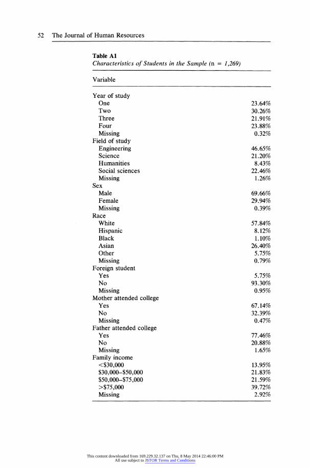
A survey of 1,269 undergraduates was carried out across all under- graduate faculties at the University of California, San Diego. Students were se- lected by a sampling of classes designed to locate students in each faculty and year of study. Engineers were oversampled due to the abundant information sources concerning engineers' salaries. The survey, which required about ten minutes of students' time, was carried out over a period of four months beginning in November 1992. Table Al at the end of the paper describes the sample.
After obtaining information on personal and family background, the survey ascertained which sources of information students had used to find out about job prospects for graduates in various fields. The survey asked students three types of questions about earnings at the national level.
1) Starting salaries. These questions were asked for workers with a bache- lor's degree in chemical, electrical, mechanical, or civil engineering (that is, four separate questions), a master's degree or Ph.D. in chemical and electrical engineering (four separate questions), bachelor's degrees in chemistry and psychology, and for a person with an MBA preceded by a technical degree (science and engineering) and a person with an MBA preceded by a nontechnical degree.
4. Some readers may question the usefulness of subjective survey data to answer these questions. But the more conventional surveys used by labor economists which examine people's choices, as opposed to beliefs, can shed no light on the information which people use. See Manski (1993) for a forceful argument in favor of using subjective data in order to analyze educational decisions.
This content downloaded from 169.229.32.137 on Thu, 8 May 2014 22:46:00 PMAll use subject to JSTOR Terms and Conditions
30 The Journal of Human Resources
2) Average salaries for engineers by their highest degree and years of experi- ence. These first two sets of questions asked for students' estimates of salaries at the time of the survey.
3) Average earnings in 1990 of "workers aged 25-34 years, working full- time" with a "high school diploma only" and those with a "bachelor's degree."5
For the exact wording of the questions, and information on response rates, see the appendix.
Students' estimates of starting salaries were compared with data on starting salaries reported in the September 1992 edition of the College Placement Coun- cil's Salary Survey, which reports national average starting salaries based on reports of 24,519 salary offers from 433 campus placement offices throughout the United States, between September 1991 and August 1992. Estimates of errors in students' beliefs about engineers' salaries by engineers' years of experience were calculated using national average salaries reported in Appendix B of the May 1992 edition of the Professional Engineer Income and Salary Survey (National Society of Professional Engineers 1992). This survey is based on 10,069 responses to the January 1992 mailing by the National Society of Professional Engineers to its members, and represents a 21.8 percent response rate. Estimated errors in students' beliefs about wages in 1990 of young workers with a bachelor's degree and those with only a high school diploma were calculated using weighted data from the March 1991 Current Population Survey.
III. An Informal Model of Educational Choice
We can shed some light on the value of labor market information to college students by considering how students choose their major in college.6 Over time, students obtain new information. Relative wages of graduates with different degrees change. Also, the student almost surely learns more about his or her abilities and interests during the college years, which reduces or changes the student's set of likely majors. One might model this as increasing dispersion in the student's beliefs about the expected utility of entering different fields as he or she progresses in college. Some students will act on new labor market information or new information about their suitability to various fields by chang- ing majors while in college. But note that changing one's major has increasing costs over time due to the sunk costs in courses taken in the original field.
This leads to several results. First, the value of information about the labor market may be greatest in the earliest years of study, since as the student pro- gresses, sunk costs and the increasing dispersion of beliefs about field-specific abilities make switching into higher-paying fields less likely. On the other hand,
5. These questions asked for estimates of wages in 1990 rather than the current year in order to facilitate comparison between the students' responses and actual wages calculated for the most recent year for which Current Population Survey data were available at the time of the study. 6. A formalization of this model is available from the author.
This content downloaded from 169.229.32.137 on Thu, 8 May 2014 22:46:00 PMAll use subject to JSTOR Terms and Conditions
Julian R. Betts 31
students, finding information costly, may decide to invest in information only at a later stage of study, after their beliefs about their suitability to various occupa- tions have evolved to the point where they have virtually ruled out many fields of study. By waiting for one or more years before learning about the labor market, students would reduce the total cost of gathering information about earnings. Thus there are countervailing forces which make it uncertain whether information acquisition should occur most intensively in the early or later years of study.
Second, it can be shown that a student will invest more in information about his or her current field of study and closely related fields, since the costs of switching to largely unrelated fields are high.
Third, the discounting of future earnings suggests that accurate knowledge of wages of inexperienced workers is more valuable than accurate knowledge about earnings of highly experienced workers.
All three of these predictions can be tested informally by examining the types of labor market information which students at different stages of college gather.
IV. Variations in Students' Beliefs about Wages
Table 1 describes the distribution of students' beliefs about salaries for each question asked. It displays the 10th, 50th, and 90th percentile wage beliefs, along with the standard deviation and the standard deviation divided by the mean. The standard deviation divided by the mean is on average 0.28. The ratio of the 90th to the 10th percentile salary estimates is typically just under 2.0. By both these measures, the variation appears to be particularly large for stu- dents' beliefs about the salaries of engineers with 15 or more years of experience.
The questionnaire explicitly asked students to estimate average salaries at the national level in the current year, rather than estimates of their own salaries. In other words, the students were making estimates of average salaries rather than their own expected salaries in given fields. Thus it seems fair to conclude that the observed differences in responses reflect substantial variation in students' information about average national salaries in each field.
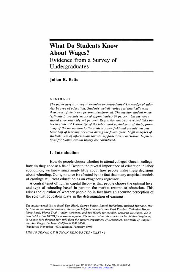
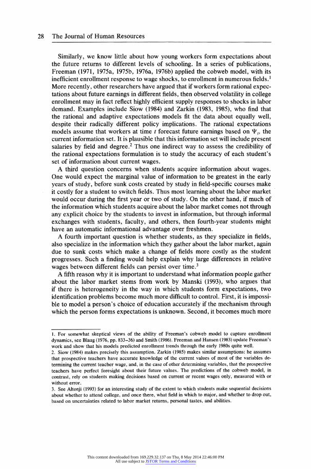
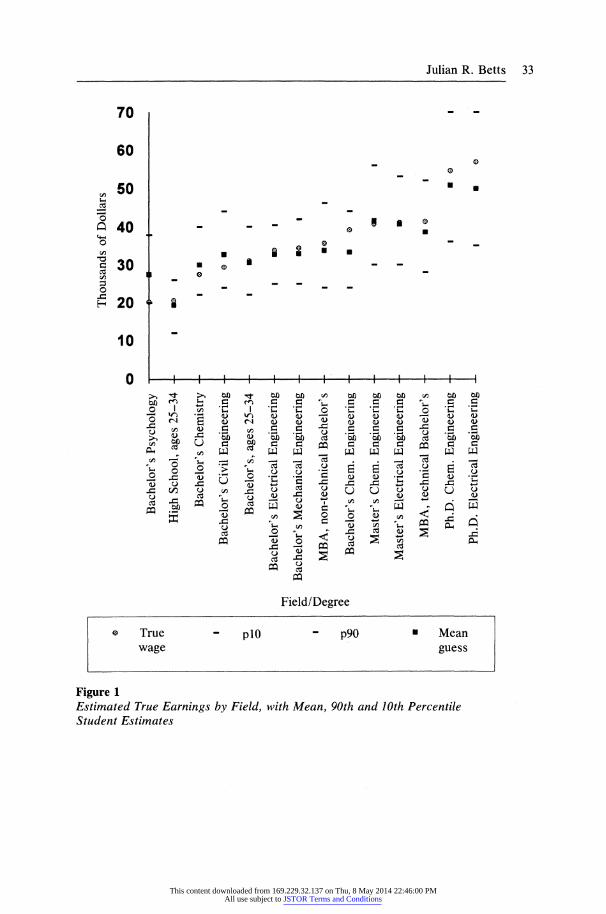
Figure 1 displays the mean, 10th, and 90th percentile estimates of annual sala- ries. The figure includes data for starting salaries for each field/degree combina- tion, as well as earnings of workers aged 25-34 who have a high school diploma only or a bachelor's degree. The figure also shows estimated "true" salaries for each question. We postpone discussion of this latter variable until the next sec- tion. The figure illustrates that wage beliefs are far from uniform. Figures 2 through 4 illustrate students' beliefs about salaries for engineers by their highest degree and years of experience, with each data point centered on the midpoint of the range of experience in question.7 These figures indicate that students do realize that wage profiles are positively sloped. They also show a large variation in students' estimates, particularly at the upper end of the experience profile.
7. There is no point on the graph for Ph.D.'s in engineering with 0-2 years' experience because the salary survey did not report this figure, apparently due to the paucity of respondents in this range.
This content downloaded from 169.229.32.137 on Thu, 8 May 2014 22:46:00 PMAll use subject to JSTOR Terms and Conditions
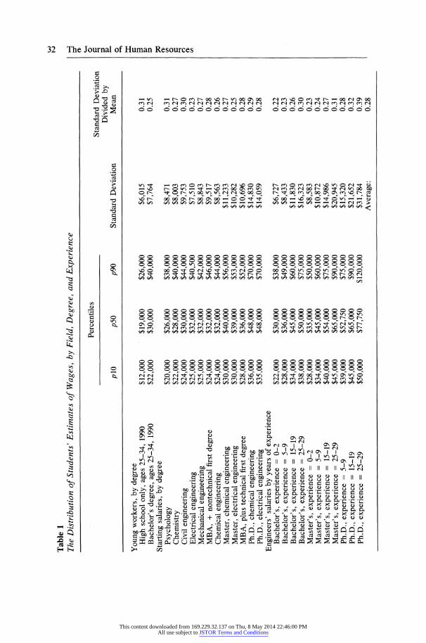
Table 1 The Distribution of Students' Estimates of Wages, by Field, Degree, and Experience
Percentiles Standard Deviation
Divided by plO p50 p90 Standard Deviation Mean
Young workers, by degree High school only, ages 25-34, 1990 Bachelor's degree, ages 25-34, 1990
Starting salaries, by degree Psychology Chemistry Civil engineering Electrical engineering Mechanical engineering MBA, + nontechnical first degree Chemical engineering Master, chemical engineering Master, electrical engineering MBA, plus technical first degree Ph.D., chemical engineering Ph.D., electrical engineering
Engineers' salaries by years of experience Bachelor's, experience = 0-2 Bachelor's, experience = 5-9 Bachelor's, experience = 15-19 Bachelor's, experience = 25-29 Master's, experience = 0-2 Master's, experience = 5-9 Master's, experience = 15-19 Master's, experience = 25-29 Ph.D., experience = 5-9 Ph.D., experience = 15-19 Ph.D., experience = 25-29
$12,000 $19,000 $22,000 $30,000
$20,000 $22,000 $24,000 $25,000 $25,000 $24,000 $24,000 $30,000 $30,000 $28,000 $36,000 $35,000
$22,000 $28,000 $34,000 $38,000 $28,000 $34,000 $40,000 $45,000 $39,000 $45,000 $50,000
$26,000 $28,000 $30,000 $32,000 $32,000 $32,000 $32,000 $40,000 $39,000 $36,000 $48,000 $48,000
$30,000 $36,000 $45,000 $50,000 $35,000 $45,000 $54,000 $65,000 $52,750 $65,000 $77,750
H
0
(-q =s
0
0 0
'-t
cn ()
CD
$26,000 $40,000
$38,000 $40,000 $44,000 $40,500 $42,000 $46,000 $44,000 $56,000 $53,000 $52,000 $70,000 $70,000
$38,000 $49,000 $60,000 $75,000 $50,000 $60,000 $75,000 $90,000 $75,000 $90,000
$120,000
$6,015 $7,764
$8,471 $8,003 $9,753 $7,510 $8,843 $9,517 $8,563
$11,233 $10,282 $10,696 $14,830 $14,059
$6,727 $8,433
$11,830 $16,323 $8,583
$10,872 $14,986 $20,945 $15,320 $21,652 $31,784
Average:
0.31 0.25
0.31 0.27 0.30 0.23 0.27 0.28 0.26 0.27 0.25 0.28 0.29 0.28
0.22 0.23 0.26 0.30 0.23 0.24 0.27 0.31 0.28 0.32 0.39 0.28
This content downloaded from 169.229.32.137 on Thu, 8 May 2014 22:46:00 PMAll use subject to JSTOR Terms and Conditions
Thousands of Dollars
0 0h 0 0 01 0 0 0 0 00, e
Bachelor's Psychology
High School, ages 25-34 -
Bachelor's Chemistry -
Bachelor's Civil Engineering -
Bachelor's, ages 25-34 -
Bachelor's Electrical Engineering
O Bachelor's Mechanical Engineering CL
CD MBA, non-technical Bachelor's -Q
^( Bachelor's Chem. Engineering
Master's Chem. Engineering
Master's Electrical Engineering
MBA, technical Bachelor's
Ph.D. Chem. Engineering
Ph.D. Electrical Engineering
I GE I
I 0
I @ I
I E I
I KG I
*e I
* ?
* 0
0n s4 0 0
C.'C
a-;L
aCCyC
O Q (DC
I O
'O
c S
C-
<- $5 3
W (T el+
w w
I
I
I
This content downloaded from 169.229.32.137 on Thu, 8 May 2014 22:46:00 PMAll use subject to JSTOR Terms and Conditions
34 The Journal of Human Resources
80
70
60
r 50 - -
l 40 -
^- _
20
10
0 5 10 15 20 25 30
Years of Experience (Mean of Interval)
-* 'True' plO p90 - - - Mean Wage Guess
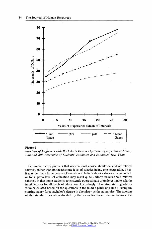
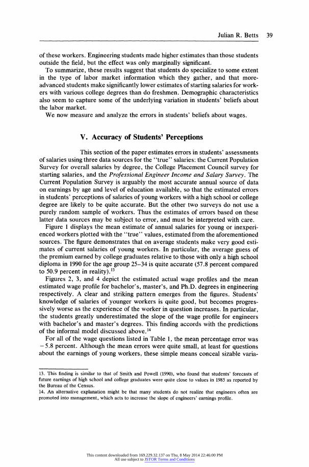
Figure 2 Earnings of Engineers with Bachelor's Degrees by Years of Experience: Mean, 10th and 90th Percentile of Students' Estimates and Estimated True Value
Economic theory predicts that occupational choice should depend on relative salaries, rather than on the absolute level of salaries in any one occupation. Thus, it may be that a large degree of variation in beliefs about salaries in a given field or for a given level of education may mask quite uniform beliefs about relative salaries, in that some students consistently overestimate or underestimate salaries in all fields or for all levels of education. Accordingly, 11 relative starting salaries were calculated based on the questions in the middle panel of Table 1, using the starting salary for a bachelor's degree in chemistry as the numeraire. The average of the standard deviation divided by the mean for these relative salaries was
This content downloaded from 169.229.32.137 on Thu, 8 May 2014 22:46:00 PMAll use subject to JSTOR Terms and Conditions
Julian R. Betts 35
90 T
80 +
70 +
2 Du -
o
0 50 - o co
c 40 -
0 30 F- 30 -
r
20 +
10 +
0
0 5 10 15 20 25 30
Years of Experience (Mean of Interval)
- 'True' plO p90 - - Mean Wage Guess
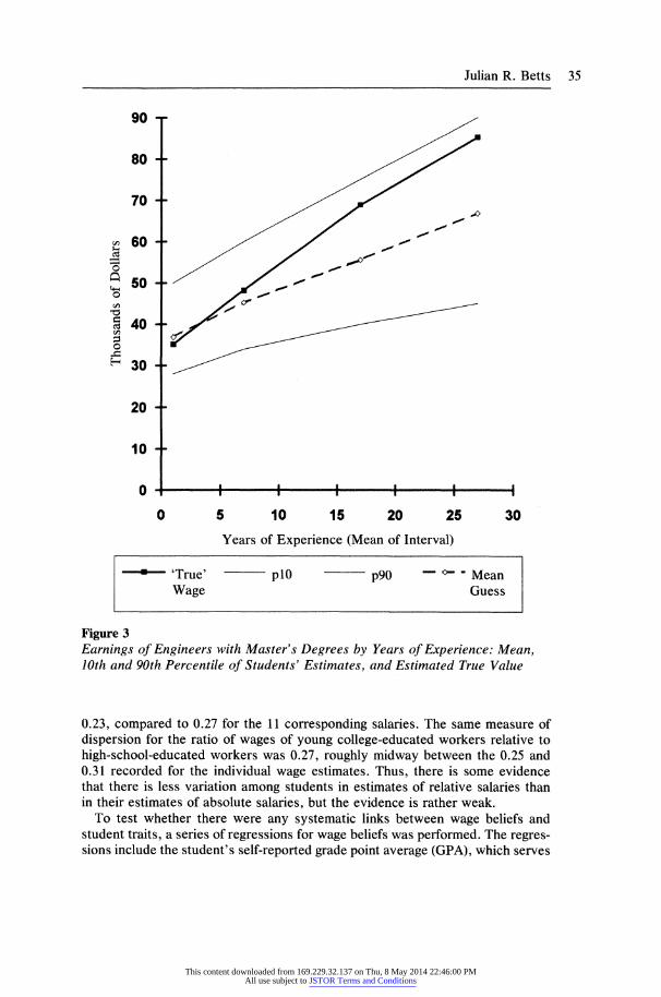
Figure 3 Earnings of Engineers with Master's Degrees by Years of Experience: Mean, 10th and 90th Percentile of Students' Estimates, and Estimated True Value
0.23, compared to 0.27 for the 11 corresponding salaries. The same measure of dispersion for the ratio of wages of young college-educated workers relative to high-school-educated workers was 0.27, roughly midway between the 0.25 and 0.31 recorded for the individual wage estimates. Thus, there is some evidence that there is less variation among students in estimates of relative salaries than in their estimates of absolute salaries, but the evidence is rather weak.
To test whether there were any systematic links between wage beliefs and student traits, a series of regressions for wage beliefs was performed. The regres- sions include the student's self-reported grade point average (GPA), which serves
.1 I
Q_
>-o/ --
?-
This content downloaded from 169.229.32.137 on Thu, 8 May 2014 22:46:00 PMAll use subject to JSTOR Terms and Conditions
36 The Journal of Human Resources
130
120
110
100
90
80
o 70 -
I 60
o 50
40
30
20
10
5 10 15 20 25 30
Years of Experience (Mean of Interval)
* 'True' pO- p90 - - Mean Wage Guess
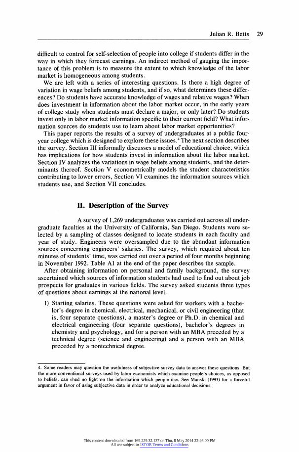
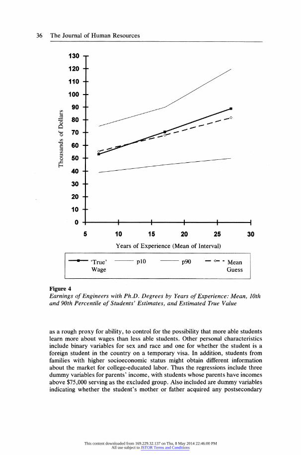
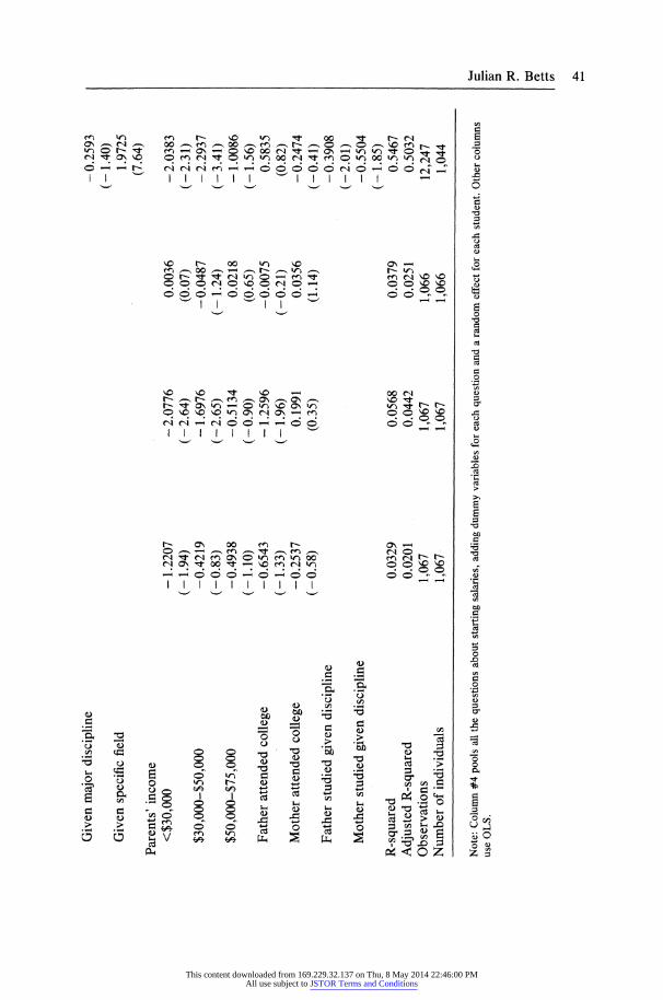
Figure 4 Earnings of Engineers with Ph.D. Degrees by Years of Experience: Mean, 10th and 90th Percentile of Students' Estimates, and Estimated True Value
as a rough proxy for ability, to control for the possibility that more able students learn more about wages than less able students. Other personal characteristics include binary variables for sex and race and one for whether the student is a foreign student in the country on a temporary visa. In addition, students from families with higher socioeconomic status might obtain different information about the market for college-educated labor. Thus the regressions include three dummy variables for parents' income, with students whose parents have incomes above $75,000 serving as the excluded group. Also included are dummy variables indicating whether the student's mother or father acquired any postsecondary
This content downloaded from 169.229.32.137 on Thu, 8 May 2014 22:46:00 PMAll use subject to JSTOR Terms and Conditions
Julian R. Betts 37
education, and whether the father or mother studied in the same major discipline (for example, engineering, science, etc.) as the wage question at hand.8
Columns 1 and 2 of Table 2 model students' beliefs about salaries in 1990 for full-time workers aged 25-34 with a high school degree only and a bachelor's degree respectively. Although the personal traits of the students have little ex- planatory power overall, several significant patterns do emerge.9 Students who are in the upper years of study tend to make lower estimates for both salaries, but the effect is much more noticeable for estimates of salaries of those with a college degree. Asian students gave significantly lower estimates of salaries for high school graduates, while black students and foreign students gave significantly higher estimates of earnings of college graduates. College attendance by a stu- dent's parents appeared to have no strong effect on either wage estimate.'0
One of the most interesting patterns is that students whose parents' income was less than $50,000 tended to make significantly lower estimates of earnings of college graduates than did students in the excluded group, which was students whose parents' income exceeded $75,000. This finding lends support to the model of Streufert (1991), which argues that young people form beliefs about the returns to education by observing workers in their neighborhood. To the extent that families segregate themselves by income, students in low-income neighborhoods should systematically underestimate the returns to education. The next section will reinforce this conclusion by showing that these students also make larger errors when estimating the salaries of young workers with a bachelor's degree.11
Smith and Powell (1990) present interesting results from a survey of 388 stu- dents at two universities. They asked students to predict earnings of both gradu- ates from their own college and their high school peers who did not attend college, for one and ten years in the future. Just as in the regressions reported here, women's estimates of earnings of high school graduates tended to be lower than those of men. Also, as in the present results, there was no statistically significant difference between men's and women's expectations for earnings of college grad- uates as a whole. But the latter result does not appear to hold in the present sample when students were asked about earnings of college-educated workers in specific fields, as will become clear below.12
8. For questions asking about engineers' salaries, these last dummy variables were set to 1 if the given parent's final field of study was engineering. Similarly, the indicator was set to 1 for the wage questions involving chemistry, psychology, and MBA's if the final parental field of study was science, humanities/ social sciences, or business respectively. 9. The OLS regressions in this table and later tables use White heteroskedastic-robust t-statistics. 10. The one exception to this last statement was that students whose fathers attended college made significantly lower estimates of the salaries of young workers with a bachelor's degree. This result is similar to that of Smith and Powell (1990). Their interpretation is that, holding family income constant, a student with a more highly educated father will underestimate the returns to college. 11. I thank a referee for bringing the paper by Streufert to my attention. 12. Perhaps the most interesting finding by Smith and Powell (1990) is that although men and women made highly similar forecasts for the earnings of college graduates, when asked to predict their own earnings men had a much higher tendency to inflate this figure relative to their estimate for their college peers than did women. Unfortunately, the questions in the present survey referred only to national averages, and not own expectations, so that I cannot attempt to replicate their finding of "self-enhanced" earnings forecasts among men.
This content downloaded from 169.229.32.137 on Thu, 8 May 2014 22:46:00 PMAll use subject to JSTOR Terms and Conditions
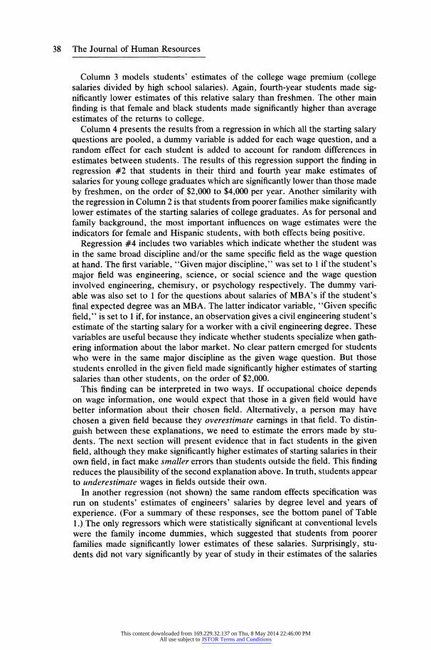
38 The Journal of Human Resources
Column 3 models students' estimates of the college wage premium (college salaries divided by high school salaries). Again, fourth-year students made sig- nificantly lower estimates of this relative salary than freshmen. The other main finding is that female and black students made significantly higher than average estimates of the returns to college.
Column 4 presents the results from a regression in which all the starting salary questions are pooled, a dummy variable is added for each wage question, and a random effect for each student is added to account for random differences in estimates between students. The results of this regression support the finding in regression #2 that students in their third and fourth year make estimates of salaries for young college graduates which are significantly lower than those made by freshmen, on the order of $2,000 to $4,000 per year. Another similarity with the regression in Column 2 is that students from poorer families make significantly lower estimates of the starting salaries of college graduates. As for personal and family background, the most important influences on wage estimates were the indicators for female and Hispanic students, with both effects being positive.
Regression #4 includes two variables which indicate whether the student was in the same broad discipline and/or the same specific field as the wage question at hand. The first variable, "Given major discipline," was set to 1 if the student's major field was engineering, science, or social science and the wage question involved engineering, chemisiry, or psychology respectively. The dummy vari- able was also set to 1 for the questions about salaries of MBA's if the student's final expected degree was an MBA. The latter indicator variable, "Given specific field," is set to 1 if, for instance, an observation gives a civil engineering student's estimate of the starting salary for a worker with a civil engineering degree. These variables are useful because they indicate whether students specialize when gath- ering information about the labor market. No clear pattern emerged for students who were in the same major discipline as the given wage question. But those students enrolled in the given field made significantly higher estimates of starting salaries than other students, on the order of $2,000.
This finding can be interpreted in two ways. If occupational choice depends on wage information, one would expect that those in a given field would have better information about their chosen field. Alternatively, a person may have chosen a given field because they overestimate earnings in that field. To distin- guish between these explanations, we need to estimate the errors made by stu- dents. The next section will present evidence that in fact students in the given field, although they make significantly higher estimates of starting salaries in their own field, in fact make smaller errors than students outside the field. This finding reduces the plausibility of the second explanation above. In truth, students appear to underestimate wages in fields outside their own.
In another regression (not shown) the same random effects specification was run on students' estimates of engineers' salaries by degree level and years of experience. (For a summary of these responses, see the bottom panel of Table 1.) The only regressors which were statistically significant at conventional levels were the family income dummies, which suggested that students from poorer families made significantly lower estimates of these salaries. Surprisingly, stu- dents did not vary significantly by year of study in their estimates of the salaries
This content downloaded from 169.229.32.137 on Thu, 8 May 2014 22:46:00 PMAll use subject to JSTOR Terms and Conditions
Julian R. Betts 39
of these workers. Engineering students made higher estimates than those students outside the field, but the effect was only marginally significant.
To summarize, these results suggest that students do specialize to some extent in the type of labor market information which they gather, and that more- advanced- students make significantly lower estimates of starting salaries for work- ers with various college degrees than do freshmen. Demographic characteristics also seem to capture some of the underlying variation in students' beliefs about the labor market.
We now measure and analyze the errors in students' beliefs about wages.
V. Accuracy of Students' Perceptions
This section of the paper estimates errors in students' assessments of salaries using three data sources for the "true" salaries: the Current Population Survey for overall salaries by degree, the College Placement Council survey for starting salaries, and the Professional Engineer Income and Salary Survey. The Current Population Survey is arguably the most accurate annual source of data on earnings by age and level of education available, so that the estimated errors in students' perceptions of salaries of young workers with a high school or college degree are likely to be quite accurate. But the other two surveys do not use a purely random sample of workers. Thus the estimates of errors based on these latter data sources may be subject to error, and must be interpreted with care.
Figure 1 displays the mean estimate of annual salaries for young or inexperi- enced workers plotted with the "true" values, estimated from the aforementioned sources. The figure demonstrates that on average students make very good esti- mates of current salaries of young workers. In particular, the average guess of the premium earned by college graduates relative to those with only a high school diploma in 1990 for the age group 25-34 is quite accurate (57.8 percent compared to 50.9 percent in reality).13
Figures 2, 3, and 4 depict the estimated actual wage profiles and the mean estimated wage profile for bachelor's, master's, and Ph.D. degrees in engineering respectively. A clear and striking pattern emerges from the figures. Students' knowledge of salaries of younger workers is quite good, but becomes progres- sively worse as the experience of the worker in question increases. In particular, the students greatly underestimated the slope of the wage profile for engineers with bachelor's and master's degrees. This finding accords with the predictions of the informal model discussed above.14
For all of the wage questions listed in Table 1, the mean percentage error was -5.8 percent. Although the mean errors were quite small, at least for questions about the earnings of young workers, these simple means conceal sizable varia-
13. This finding is similar to that of Smith and Powell (1990), who found that students' forecasts of future earnings of high school and college graduates were quite close to values in 1985 as reported by the Bureau of the Census. 14. An alternative explanation might be that many students do not realize that engineers often are promoted into management, which acts to increase the slope of engineers' earnings profile.
This content downloaded from 169.229.32.137 on Thu, 8 May 2014 22:46:00 PMAll use subject to JSTOR Terms and Conditions
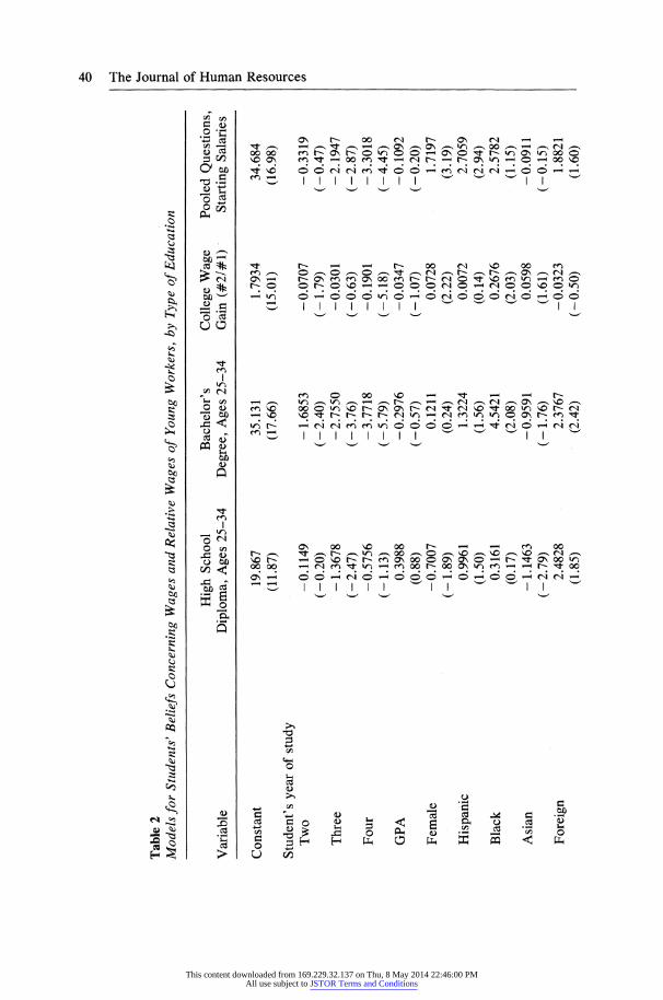
Table 2 Models for Students' Beliefs Concerning Wages and Relative Wages of Young Workers, by Type of Education
High School Bachelor's College Wage Pooled Questions, Variable Diploma, Ages 25-34 Degree, Ages 25-34 Gain (#2/#1) Starting Salaries
Constant
Student's year of study Two
Three
Four
GPA
Female
Hispanic
Black
Asian
Foreign
19.867 (11.87)
-0.1149 (-0.20) - 1.3678
(-2.47) -0.5756
(-1.13) 0.3988
(0.88) - 0.7007
(-1.89) 0.9961
(1.50) 0.3161
(0.17) - 1.1463
(-2.79) 2.4828
(1.85)
35.131 (17.66)
- 1.6853
(-2.40) - 2.7550
(-3.76) - 3.7718
(-5.79) -0.2976
(-0.57) 0.1211
(0.24) 1.3224
(1.56) 4.5421
(2.08) -0.9591
(-1.76) 2.3767
(2.42)
1.7934 (15.01)
- 0.0707 (-1.79) - 0.0301
(-0.63) -0.1901
(-5.18) -0.0347
(-1.07) 0.0728
(2.22) 0.0072
(0.14) 0.2676
(2.03) 0.0598
(1.61) - 0.0323
(-0.50)
34.684 (16.98)
- 0.3319 (-0.47) -2.1947
(-2.87) - 3.3018
(-4.45) -0.1092
(-0.20) 1.7197
(3.19) 2.7059
(2.94) 2.5782
(1.15) -0.0911
(-0.15) 1.8821
(1.60)
0
0
3
c rt
(r-
This content downloaded from 169.229.32.137 on Thu, 8 May 2014 22:46:00 PMAll use subject to JSTOR Terms and Conditions
Given major discipline - 0.2593 (-1.40)
Given specific field 1.9725 (7.64)
Parents' income <$30,000 -1.2207 -2.0776 0.0036 - 2.0383
(-1.94) (-2.64) (0.07) (-2.31) $30,000-$50,000 -0.4219 -1.6976 -0.0487 -2.2937
(-0.83) (-2.65) (-1.24) (-3.41) $50,000-$75,000 -0.4938 -0.5134 0.0218 -1.0086
(- 1. 10) (-0.90) (0.65) (-1.56) Father attended college -0.6543 - 1.2596 -0.0075 0.5835
(-1.33) (-1.96) (-0.21) (0.82) Mother attended college -0.2537 0.1991 0.0356 -0.2474
(-0.58) (0.35) (1.14) (-0.41) Father studied given discipline - 0.3908
(-2.01) Mother studied given discipline -0.5504
(-1.85) R-squared 0.0329 0.0568 0.0379 0.5467 Adjusted R-squared 0.0201 0.0442 0.0251 0.5032 Observations 1,067 1,067 1,066 12,247 Number of individuals 1,067 1,067 1,066 1,044
Note: Column #4 pools all the questions about starting salaries, adding dummy variables for each question and a random effect for each student. Other columns - use OLS.
?T?
C,
This content downloaded from 169.229.32.137 on Thu, 8 May 2014 22:46:00 PMAll use subject to JSTOR Terms and Conditions
42 The Journal of Human Resources
tions in the accuracy of the students' beliefs. The median of the absolute percent- age errors is a better measure of the errors typically made than is the mean of the signed errors. The average of these medians across all wage questions shown in Table 1 is 19.6 percent, compared to -5.8 percent for the raw mean.
Furthermore, not one student accurately ranked all 14 earnings levels. But perhaps a fairer test is to examine the proportion of students correctly ranking four jobs with quite highly dispersed salaries: jobs of those with an MBA preceded by a science or engineering bachelor's degree, and bachelor's degrees in mechani- cal engineering, chemistry, and psychology. If all students had guessed randomly due to a lack of information, we would expect just 4.2 percent [that is, (100 percent)/4!] to have answered correctly. If all students had possessed complete information, then 100 percent should have answered accurately. Of 1,163 students who answered the questions, 26.3 percent ranked these salaries correctly. Thus, students do know something about salaries, but they fall far short of having complete information.15
What determines students' errors in perception? To answer this question, we now econometrically model the students' errors. See Table 3. It is not useful to make the signed error the dependent variable, since a positive coefficient on regressor x could indicate that a higher value of x is associated with a higher positive error, a smaller negative error, or both.16 Therefore the following series of regressions examines the absolute value of errors, in order to determine what factors influence the actual size of errors in absolute terms. The dependent vari- able is the log of the absolute value of the percentage wage error:17
(west - wtrue) x 1o00 ln wtrue
The basic regression uses the same set of wage questions and regressors used to model wage beliefs in Table 2. The first two columns model absolute errors in
15. As mentioned in the previous section, large absolute errors in students' beliefs about a given salary may conceal relatively small errors in their estimates of relative salaries. This does not appear to be the case, though. When all of the salaries in the top two panels of Table 1 were converted to relative salaries using the salary of those with a bachelor's degree in chemistry as the numeraire, estimates of relative errors were quite similar, but were slightly higher in 11 of 13 cases. Using the starting salary for a Ph.D. in electrical engineering as numeraire produced similar results. 16. Consider the following example to see why modeling signed errors is not useful. Suppose women are equally divided into those making a - 1 percent error or a + 2 percent error, while men are equally divided into those making a - 50 percent error and a + 50 percent error. Regression of signed errors on a dummy for male would give a negative coefficient, incorrectly implying that the typical man made smaller errors than the typical woman. In contrast, if we use the absolute error as the dependent variable, then the coefficient on the male dummy would be positive, indicating (correctly) that the typical male makes larger errors. 17. The log absolute error is used as the dependent variable since the absolute values themselves are positive, which would have rendered the normality assumption used for inference in OLS highly untena- ble. Comparison of the log likelihood values for both linear and log versions of the dependent variable (after adjusting for the Jacobian term) showed the log specification to be superior in almost all regressions involving starting salaries, and for five of 11 regressions in Table A2. Estimates using the linear absolute percentage errors, which are available from the author on request, show highly similar results to those outlined below. Another advantage of the log specification, of course, is that it lessens the influence of outliers.
This content downloaded from 169.229.32.137 on Thu, 8 May 2014 22:46:00 PMAll use subject to JSTOR Terms and Conditions
Julian R. Betts 43
students' estimates of 1990 salaries of young full-time workers who have a high school diploma only or a bachelor's degree respectively. Since the "true" values for these salaries were calculated using the most reliable data source of the three used-the Current Population Survey-it is for these questions that we can have most confidence that we are accurately measuring errors in students' beliefs.
For both wage questions, students' errors tend to decline with year of study. But the differences become significant only between fourth-year and first-year students' errors in estimating the earnings of high school graduates. This result suggests continual learning about the labor market.18
A second notable finding is that students from poorer families made significantly larger errors estimating salaries of college graduates. The results in Table 2 indi- cate that this difference stems from students from poorer families underestimating the earnings of college graduates. The finding of a negative correlation between students' errors and parents' income has at least three possible interpretations. The first is that higher family income itself buys better information. Second, since lower income is often associated with retirement or families in which only one parent works, it may be that a working parent provides a child with a valuable window into the workplace. Third, the aforementioned model by Streufert (1991) of geographic sorting of families by income may explain the result: children from poorer neighborhoods may underestimate the returns to college due to a lack of information.
Column 3 models log absolute errors in students' estimates of the earnings of young college graduates relative to the earnings of young high school graduates. This regression reveals that fourth-year students appear to make significantly smaller errors than freshmen, which we interpret as another sign of learning. 19
Column 4 models the estimated log absolute error in all starting salary ques- tions. A random effect is added to account for repeated observations for students, and dummy variables are added for each question.20
The effect of year of study is highly similar to that in the regressions in Columns 1-3, but the coefficients are far more significant. Absolute errors decrease mono- tonically with year of study, with well over half of learning occurring among fourth-year students. The conclusion that most learning about the labor market occurs late in the student's college career runs against the predictions of the informal model discussed earlier, but as noted there, is consistent with the idea that students wait until they have learned about their abilities before investing in
18. One referee suggested that once a student has started college, she will have no further use for investing in information about the earnings of high school graduates. The results here suggest that college students do in fact learn more about the earnings of high school graduates as they progress through college. One possible explanation is that many of the information sources which students use, such as newspaper articles, often report earnings for college graduates alongside those for less educated workers. In other words, it may not be entirely possible to unbundle information acquisition. 19. To test whether a few particularly large wage errors were influencing these three regressions, the method proposed by Krasker et al. (1983) was used to remove influential observations, after which the regressions were repeated. No important changes resulted, except that the coefficient on the dummy variable for blacks became unidentified due to the small sample of blacks in the data set. 20. An nR2 test for exclusion of the dummy variables rejected the null with a p-value less than 0.000005. Regressions without the random effect for individuals produced highly similar coefficients, but the t- statistics were in general higher.
This content downloaded from 169.229.32.137 on Thu, 8 May 2014 22:46:00 PMAll use subject to JSTOR Terms and Conditions
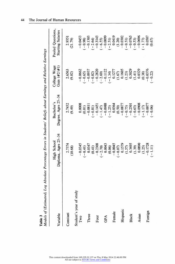
Table 3 Models of (Estimated) Log Absolute Percentage Errors in Students' Beliefs about Earnings and Relative Earnings
High School Bachelor's College Wage Pooled Questions, Variable Diploma, Ages 25-34 Degree, Ages 25-34 Gain (#2/#1) Starting Salaries
Constant
Student's year of study Two
Three
Four
GPA
Female
Hispanic
Black
Asian
Foreign
2.7374 (10.68)
-0.0345 (-0.41)
0.0347 (0.41)
-0.2308 (-2.70)
0.0043 (0.06)
-0.0045 (-0.07)
0.1579 (1.57) 0.3695
(1.39) 0.0890
(1.25) -0.1728
(-1.11)
2.7432 (9.49)
0.0008 (0.01)
- 0.0811 (-0.81) -0.1451
(-1.47) - 0.0988
(-1.25) 0.0364
(0.50) -0.0877
(-0.75) - 0.2501
(-0.63) - 0.0908
(-1.17) - 0.0077
(-0.06)
2.6563 (9.02)
- 0.0662 (-0.65) -0.0937
(-0.82) -0.2820
(-2.69) -0.1122
(-1.34) 0.1277
(1.67) 0.1605
(1.23) 0.5029
(1.41) 0.0329
(0.38) - 0.0376
(-0.22)
2.9351 (21.79)
- 0.0453 (-0.98) -0.1303
(- 2.64) - 0.3143
(- 6.55) - 0.0899
(-2.51) 0.0419
(1.20) - 0.0302
(-0.51) - 0.0765
(-0.53) - 0.0696
(-1.77) 0.0507
(0.67)
t- 0
0
~1 i,,
E= gO
Cn
This content downloaded from 169.229.32.137 on Thu, 8 May 2014 22:46:00 PMAll use subject to JSTOR Terms and Conditions
Given major discipline -0.0872 (-3.55)
Given specific field -0.1117 (-3.06)
Parents' income <$30,000 0.0697 0.2364 0.1302 0.0821
(0.68) (2.29) (1.08) (1.44) $30,000-$50,000 0.0305 0.1869 0.0566 0.0124
(0.39) (2.13) (0.59) (0.29) $50,000-$75,000 0.0913 -0.0103 0.0911 -0.0312
(1.20) (-0.12) (1.01) (-0.75) Father attended college 0.0629 0.1398 0.1517 0.0133
(0.75) (1.44) (1.45) (0.29) Mother attended college -0.0843 0.0067 0.1003 0.0339
(-1.21) (0.08) (1.11) (0.86) Father studied given discipline -0.0421
(-1.61) Mother studied given discipline -0.1382
(-3.32) R-squared 0.0203 0.0140 0.0208 0.0547 Adjusted R-squared 0.0072 0.0008 0.0077 -0.0360 Observations 1,067 1,067 1,066 12,247 Number of individuals 1,067 1,067 1,066 1,044 LM (nR2) test for exclusion of 0.311
(year) (given field) interac- tions (p-value)
Note: See notes to Table 2.
'i,
This content downloaded from 169.229.32.137 on Thu, 8 May 2014 22:46:00 PMAll use subject to JSTOR Terms and Conditions
46 The Journal of Human Resources
information. Also, as one referee pointed out, those fourth-year students who already had ajob offer at the time of the survey (in late fall and early winter) could have learned about earnings, at least in their own area, directly from employers.
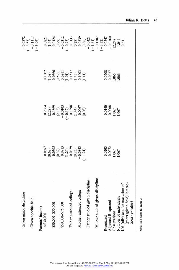
Students who are in the same "major discipline" as the occupation in question make significantly lower errors, by about 8.7 log points, while those who are in the specific discipline make even smaller errors, with a further reduction in the average error by 11.2 log points. Taken together, the implication is that a student in the specific field, such as chemical engineering, on average makes errors which are only 0.82 as large as students outside of engineering altogether.21
The informal model suggested that students might increasingly specialize in information acquisition as they progress through college, since the costs of trans- ferring to other fields rise. The bottom of the table reports results of tests for the exclusion of two interaction terms between the year of study and the dummy variables for the student being in the given field and the given area. The restric- tions were easily retained, so that the data do not give evidence of an increase in specialization as students progress.
Somewhat surprisingly, the coefficients on the measures of parental education are not significant, although there is evidence that students whose mother studied in the given field made significantly smaller errors.
Finally, students with higher GPAs appear to make significantly lower errors when estimating starting salaries. It is not clear whether GPA may be acting as an ability proxy in this model.22
The theoretical discussion in Section III suggested that students will be more willing to invest in information about starting salaries than about salaries of highly experienced workers, due to the discounting of future income. The figures dis- cussed earlier indicate that this hypothesis is correct. More formally, regressions in Table A2 in the appendix model estimated errors in students' beliefs about current salaries of engineers by years of experience.23 The regressions suggest
21 In other words, instead of making a 10 percent error, an engineer might make an error of 0.82 (10 percent) or 8.2 percent. 22. As a test of robustness, the models in Table 3 were reestimated using the proportional errors squared rather than the log of the absolute values of the errors. For the regressions in Columns 1 and 3, no coefficient crossed from being significant (that is, t I > 1.96) to insignificant or vice versa. In regression #2, the coefficient on the dummy for students in their fourth year of study became negative and signifi- cant at the 5 percent level, while the family income variables became insignificant. In the pooled regres- sion, the only crucial change was that the dummies for whether the student was in the specific field or major discipline became insignificantly different from zero. However, it became apparent that the squar- ing of the errors had created outlier problems which contributed to the latter changes. Thus observations were deleted if the squared error was greater than 0.5. (This corresponds to percentage errors greater than 70.7 percent.) In the remaining sample, containing 97 percent of the original observations, the dummy for study in the major discipline became significant (t = -3.10) and the dummy for study in the given field became moderately significant (t = - 1.77) again. Thus the overall patterns such as specialization by field and learning over time appear quite robust to the choice of dependent variable. 23. The response rate on these questions was 77-78 percent, compared to 93-97 percent for the ques- tions on starting salaries. One reason for the drop in response rate may simply be that these questions appeared at the end of the survey. But two of the students who did not fill out these questions on engineers' salaries by years of experience indicated on the form that they had "no idea" what the wage profiles looked like.
This content downloaded from 169.229.32.137 on Thu, 8 May 2014 22:46:00 PMAll use subject to JSTOR Terms and Conditions
Julian R. Betts 47
that students invest more in information about starting wages than they do about wages of highly experienced workers. The regressions show that students learn about the labor market over time, and that engineering students do know more about salaries of engineers. But these relations break down when students are asked about salaries of engineers with 15-19 and 25-29 years of experience, where no pattern of learning or specialization is discernible.
In summary, although our estimates of students' errors in wage beliefs are based on our own possibly biased estimates of the "true" values, the results provide mostly intuitive results. In particular, students do specialize in the acqui- sition of labor market information, even at an early date of study. Second, they learn more about the labor market as they progress. Third, the discussion of theory in Section III implied that students will invest more in information about the earnings of younger workers than older workers, due to discounting of future income. This idea gains support from errors in the students' estimates of the earnings of engineers by years of experience.
VI. Information Sources Used by Students
While the above analysis proves that observable student character- istics are associated with students' beliefs about the labor market, it does not provide any direct evidence about why certain students are better informed. For instance, why do fourth-year students seem to know more about the labor market than their younger colleagues? Does it reflect active search for information or merely learning by osmosis which automatically occurs over time?
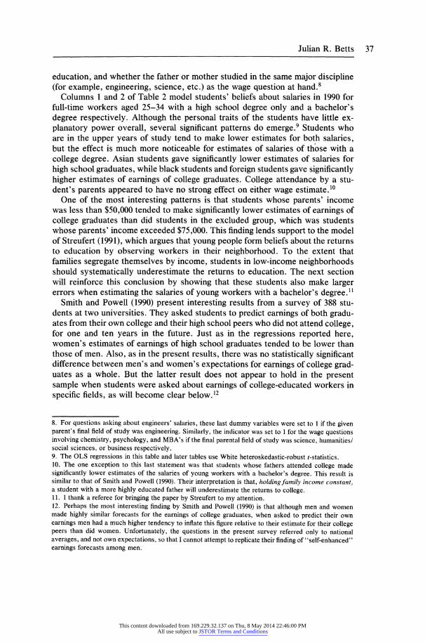
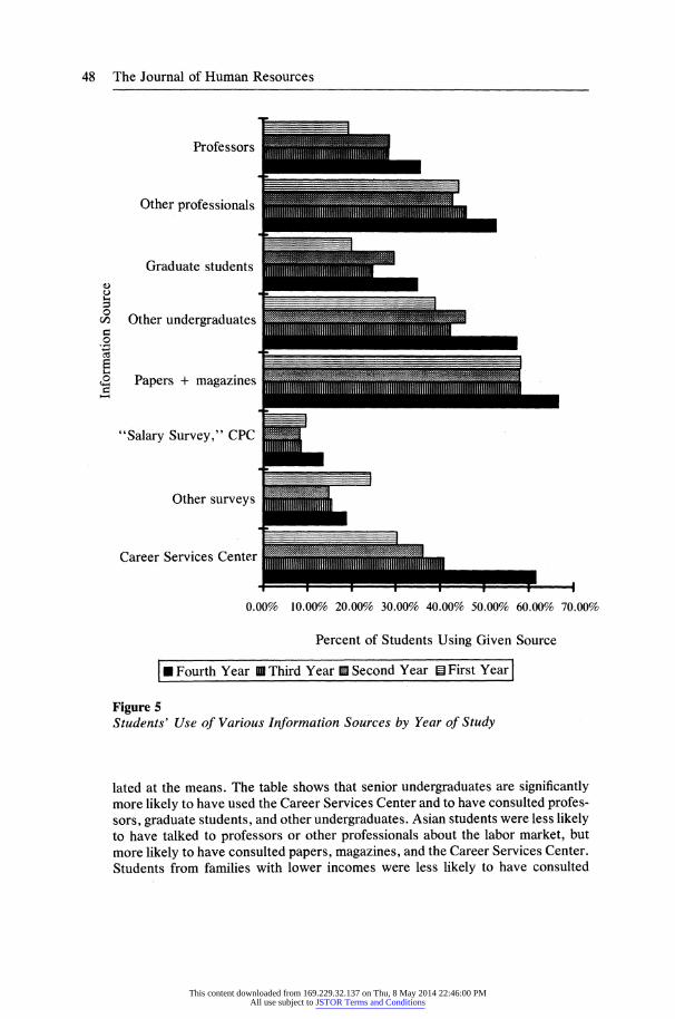
To this end, the survey asked students to indicate which information sources they had used to "find out about job prospects of graduates in various fields." The distribution of responses by year of study appears in Figure 5.24
As the figure shows, by far the most commonly used source of information is newspapers and magazines. Surprisingly few students report consulting profes- sors, graduate students, or salary surveys for information.
In all but one case there is a large increase in the proportion of students using each information source in the fourth year of study. This pattern is especially strong for use of the campus Career Services Center. It appears that this Center is not used by a majority of students until their fourth year of study, implying that the Center serves less to help students choose a field than it does to provide information about jobs to those who are about to graduate.
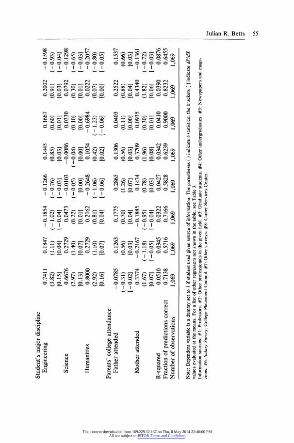
In order to model the determinants of the use of each of these eight information sources more formally, while controlling for possible collinearity between year of study and other student traits, logit models were estimated for each source of information. Table A-3 in the appendix shows the estimated coefficients, t- statistics, and, in square brackets below the t-statistics, the dPIdX values calcu-
24. Students were specifically asked whether they had consulted the Salary Survey of the College Placement Council both because this survey is readily available at the campus placement center and because it was used above to calculate errors in students' estimates of starting salaries.
This content downloaded from 169.229.32.137 on Thu, 8 May 2014 22:46:00 PMAll use subject to JSTOR Terms and Conditions
48 The Journal of Human Resources
Professors
Other professionals
Other undergraduates
Papers + magazines
"Salary Survey," CPC
Other surveys
Percent of Students Using Given Source
* Fourth YearU0 Third Year M Second YearElFirst YearI
Figure 5 Students' Use of Various Information Sources by Year of Study
lated at the means. The table shows that senior undergraduates are significantly more likely to have used the Career Services Center and to have consulted profes- sors, graduate students, and other undergraduates. Asian students were less likely to have talked to professors or other professionals about the labor market, but more likely to have consulted papers, magazines, and the Career Services Center. Students from families with lower incomes were less likely to have consulted
0 C
C a
'EZ c Uk c c
4w
This content downloaded from 169.229.32.137 on Thu, 8 May 2014 22:46:00 PMAll use subject to JSTOR Terms and Conditions
Julian R. Betts 49
professors or other professionals. Finally, the variables measuring parents' educa- tion in general had little effect.25
Thus, this section sheds some light on the reasons for the significant correla- tions observed earlier between errors in wage estimates and personal background. But, given that in many cases the logits successfully predict only about 60 percent of the responses, there is much that remains to be learned about how, for exam- ple, more senior students hone their knowledge of wages.26
VII. Summary and Conclusion
The above results provide answers to many of the questions set out in the introduction. First, students do have diverse beliefs about the labor market, as is shown in Section IV. These differences in beliefs are systematically linked to personal traits such as year and field of study.
Second, estimates of students' median absolute errors in wage beliefs were typically about 20 percent. But the mean of the estimated raw errors was very small, averaging only about -6 percent, as some students overestimated the salary in a given job while others underestimated it.
Third, two implications of the informal model were borne out by the data. Students specialized in acquiring information about earnings of workers in their own major discipline and subfield. This finding suggests the presence of sunk costs related to field-specific human capital. The second implication of the model was that students should find it more worthwhile to invest in information about earnings of young workers, due to discounting. The results support this hy- pothesis.
Third, the regression results indicate that fourth-year students knew signifi- cantly more about salary levels than first year students. On average over half of the learning between the first and fourth year of study occurred in the final year. This conclusion is supported by logit analyses of the determinants of the use of specific sources of labor market information, such as the campus placement cen- ter, which showed a significant increase in usage of a broad array of information sources during the fourth year of study. In contrast, the informal model had predicted that students might find it most worthwhile to invest in labor market information at an earlier stage. Possible explanations for the discrepancy include postponement of research into the labor market until the student has narrowed down the list of potential fields of study (due to the cost of information), and the automatic learning which occurs when fourth-year students begin to apply for jobs.
25. Repetition of the logit regressions without the dummies for parents' field(s) of specialization had little effect on the results, leaving the significance of the two dummies for college attendance by the parents little changed. 26. As another way of seeing this point, consider the fact that when the regressions in Table 3 were repeated with dummy variables for use of each source of information as additional regressors, the coefficients and t-statistics on the other regressors were little changed. (However, interpretation of these regressions is difficult, given the obvious endogeneity of the information-source variables.)
This content downloaded from 169.229.32.137 on Thu, 8 May 2014 22:46:00 PMAll use subject to JSTOR Terms and Conditions
50 The Journal of Human Resources
The finding that students differ significantly in their beliefs about wages in different fields deserves further comment. It implies that students will also form diverse expectations of future returns to education in various fields. As shown by Manski (1993), in such a world conventional methods of estimating the returns to schooling are likely to be biased.27
Indeed, the above findings raise doubts about the assumption made in some rational expectations versions of the human capital model that students forecast future wages based on accurate knowledge of current wages. Information is far from complete. For instance, only 26 percent of students accurately ranked four jobs by starting salary, compared to 4 percent in the case of purely random guessing and 100 percent in the case of perfect information. It is unlikely that these errors reflect measurement error alone: the regression analysis found sys- tematic differences in wage errors between students suggestive of, for instance, learning over time.
Two other branches of research point in the same direction. The Government Accounting Office (1990) reviews a series of papers which find large gaps in what high school students and their parents know about postsecondary financial aid and college costs, and suggests that this lack of information may prevent families from making fully rational educational decisions. Similarly, Leonard (1982) uses data from an annual survey of employers' wage expectations, and in most cases strongly rejects the hypothesis of rational expectations.
But taken as a whole, the above findings strongly support the assumption made by human capital theory that workers acquire information about earnings by level of education in order to choose their optimal level of education. Information is not perfect, but a process of learning over time is clearly discernible.
The findings of this study suggest that it would be worthwhile for economists to study the acquisition of labor market information in a panel format. A repeated survey of young workers over several years could yield important new insights into how people learn about the labor market and the ways in which this learning informs their subsequent decisions about education.
Appendix 1
Description of Survey Instrument
The survey begins with 16 background questions in multiple choice format, which is followed by a section asking students to estimate salaries in various fields.
For the questions on starting salaries students were given a list of 44 salaries in increments of $2,000, that is, "14 16 . . . 100," and were asked to circle the
appropriate salary for the given occupation and level of education in each case. This list of salaries was used in order to minimize "rounding error," that is, rough estimates such as $30,000, $40,000, etc. In addition, the survey stated "If your estimate lies in between two of the printed numbers, insert an arrow in
27. Manski also shows that even if all students have identical information, inference can still be biased in the case in which the researcher misspecifies the information set.
This content downloaded from 169.229.32.137 on Thu, 8 May 2014 22:46:00 PMAll use subject to JSTOR Terms and Conditions
Julian R. Betts 51
between, e.g. indicate an estimate of $25,000 by writing '22 24 J 26.' If your estimate lies outside the limits printed below, please write in your estimate by hand. Please make an estimate for all of the following, even if you are unsure."
The exact wording for the questions on starting salaries was "Below, please circle your estimate of the national average for annual starting salaries (in thou- sands of dollars) of graduates in the indicated fields and degree levels during this year." (Emphasis is as in the survey form). The overall response rate on these questions was 94.4 percent.
Similar wording was used for the questions about annual salaries in 1990 of workers aged 25-34 by highest degree. The response rate for these questions was 96.9 percent. For these two questions, students were asked to estimate earnings in 1990, because at the time of the survey 1990 was the most recent year for which data from the March Current Population Survey were available for purposes of comparison.
For all of these questions described above, there was some evidence of "rounding error," although students on the whole provided fairly precise esti- mates. For instance, 25.1 percent of estimates were exact multiples of $10,000, and 77.4 percent of estimates were multiples of $2,000. (Recall that the scale written on the survey form displayed salaries in even increments of $2,000.)
For the questions about salaries of engineers by level of education and years of experience, the instructions read: "The table below classifies engineers by their highest degree and their years of work experience since their final degree. In each box, please write your best estimate of the current ANNUAL SALARY of the given type of engineer." The overall response rate for these questions was 77.2 percent. Of these, 35.4 percent consisted of estimates which were exact multiples of $10,000.
This content downloaded from 169.229.32.137 on Thu, 8 May 2014 22:46:00 PMAll use subject to JSTOR Terms and Conditions
52 The Journal of Human Resources
Table Al Characteristics of Students in the Sample (n = 1,269)
Variable
Year of study One 23.64% Two 30.26% Three 21.91% Four 23.88% Missing 0.32%
Field of study Engineering 46.65% Science 21.20% Humanities 8.43% Social sciences 22.46% Missing 1.26%
Sex Male 69.66% Female 29.94% Missing 0.39%
Race White 57.84% Hispanic 8.12% Black 1.10% Asian 26.40% Other 5.75% Missing 0.79%
Foreign student Yes 5.75% No 93.30% Missing 0.95%
Mother attended college Yes 67.14% No 32.39% Missing 0.47%
Father attended college Yes 77.46% No 20.88% Missing 1.65%
Family income <$30,000 13.95% $30,000-$50,000 21.83% $50,000-$75,000 21.59% >$75,000 39.72% Missing 2.92%
This content downloaded from 169.229.32.137 on Thu, 8 May 2014 22:46:00 PMAll use subject to JSTOR Terms and Conditions
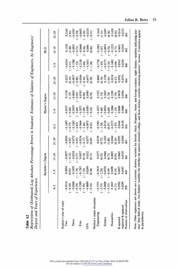
Table A2 Regressions of (Estimated) Log Absolute Percentage Errors in Students' Estimates of Salaries of Engineers, by Engineers' Degree and Years of Experience
Bachelor's Degree Master's Degree Ph.D.
0-2 5-9 15-19 25-29 0-2 5-9 15-19 25-29 5-9 15-19 25-29
Student's year of study Two -0.0116 0.0034 -0.0077 -0.0024 -0.1092 -0.0557 0.1128 0.0227 -0.0314 0.1320 0.2142
(-0.10) (0.03) (-0.12) (-0.03) (-0.75) (-0.60) (1.25) (0.24) (-0.31) (1.09) (1.83) Three -0.0368 -0.1939 -0.0234 -0.0772 -0.1263 -0.3019 -0.0045 -0.0917 -0.1590 -0.0923 -0.0507
(-0.29) (-1.76) (-0.37) (-0.95) (-0.85) (-3.04) (-0.05) (-0.88) (-1.52) (-0.71) (-0.39) Four -0.2389 -0.1265 0.0057 -0.0134 -0.3644 -0.2872 0.0743 -0.0164 -0.2138 -0.0448 -0.0492
(-1.93) (-1.24) (0.10) (-0.17) (-2.46) (-2.99) (0.80) (-0.16) (-2.09) (-0.36) (-0.39) GPA -0.0089 0.0249 0.0322 0.0377 -0.0973 -0.0383 0.0385 0.0477 -0.1031 0.0481 -0.0224
(-0.10) (0.30) (0.71) (0.69) (-0.93) (-0.54) (0.59) (0.78) (-1.28) (0.46) (-0.31) Student's major discipline
Engineering -0.3535 -0.2018 0.0175 0.0539 -0.3305 -0.3075 0.1322 0.0683 -0.1728 -0.1963 0.1610 (-3.55) (-2.26) (0.32) (0.72) (-2.50) (-3.68) (1.53) (0.70) (-1.95) (-1.87) (1.55)
Science -0.0408 -0.0529 0.0460 0.1623 0.0110 -0.0654 0.1823 0.1750 -0.0172 -0.0974 0.0497 (-0.35) (-0.50) (0.71) (1.88) (0.07) (-0.68) (1.79) (1.61) (-0.16) (-0.76) (0.38)
Humanities 0.1845 0.0498 0.0893 0.0360 -0.2275 -0.2004 0.2182 0.0318 -0.1492 -0.1235 0.1420 (1.21) (0.35) (0.93) (0.26) (-1.05) (-1.33) (1.59) (0.17) (-0.99) (-0.77) (0.92)
R-squared 0.0582 0.0437 0.0645 0.0595 0.0446 0.0684 0.0678 0.0562 0.0543 0.0631 0.0514 Adjusted R-squared 0.0299 0.0147 0.0359 0.0309 0.0158 0.0400 0.0394 0.0274 0.0256 0.0345 0.0223 Number of observations 858 849 845 847 854 848 846 844 848 845 843
Note: Other regressors not shown are a constant, dummy variables for female, black, Hispanic, Asian, and foreign students, eight dummy variables indicating par- ents' final field of study, two dummy variables for whether the parents attended college, and three dummy variables indicating parents' income. T-statistics appear in parentheses.
t*
CD
cn
tn
el+
(-A (^
This content downloaded from 169.229.32.137 on Thu, 8 May 2014 22:46:00 PMAll use subject to JSTOR Terms and Conditions
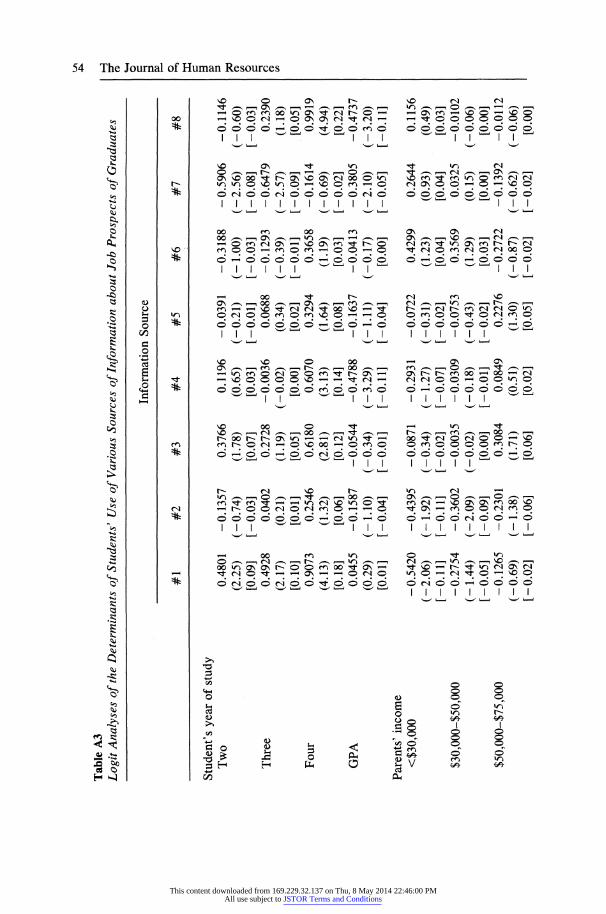
Table A3 Logit Analyses of the Determinants of Students' Use of Various Sources of Information about Job Prospects of Graduates
Information Source
#1 #2 #3 #4 #5 #6 #7 #8
Student's year of study Two
Three
Four
GPA
Parents' income <$30,000
$30,000-$50,000
$50,000-$75,000
0-3 3
s,
-
0
5=
co CD> c/
0.4801 -0.1357 0.3766 0.1196 -0.0391 -0.3188 -0.5906 -0.1146 (2.25) (-0.74) (1.78) (0.65) (-0.21) (-1.00) (-2.56) (-0.60) [0.09] [-0.03] [0.07] [0.03] [-0.01] [-0.03] [-0.08] [-0.03] 0.4928 0.0402 0.2728 -0.0036 0.0688 -0.1293 -0.6479 0.2390
(2.17) (0.21) (1.19) (-0.02) (0.34) (-0.39) (-2.57) (1.18) [0.10] [0.01] [0.05] [0.00] [0.02] [-0.01] [-0.09] [0.05] 0.9073 0.2546 0.6180 0.6070 0.3294 0.3658 -0.1614 0.9919
(4.13) (1.32) (2.81) (3.13) (1.64) (1.19) (-0.69) (4.94) [0.18] [0.06] [0.12] [0.14] [0.08] [0.03] [-0.02] [0.22] 0.0455 -0.1587 -0.0544 -0.4788 -0.1637 -0.0413 -0.3805 -0.4737
(0.29) (- 1. 10) (-0.34) (- 3.29) (- 1.11) (-0.17) (- 2.10) (- 3.20) [0.01] [-0.04] [-0.01] [-0.11] [-0.04] [0.00] [-0.05] [-0.11]
-0.5420 -0.4395 -0.0871 -0.2931 -0.0722 0.4299 0.2644 0.1156 (-2.06) (-1.92) (-0.34) (-1.27) (-0.31) (1.23) (0.93) (0.49) [-0.11] [-0.11] [-0.02] [-0.07] [-0.02] [0.04] [0.04] [0.03] -0.2754 -0.3602 -0.0035 -0.0309 -0.0753 0.3569 0.0325 -0.0102
(- 1.44) (-2.09) (-0.02) (-0.18) (-0.43) (1.29) (0.15) (-0.06) [-0.05] [-0.09] [0.00] [-0.01] [-0.02] [0.03] [0.00] [0.00] -0.1265 -0.2301 0.3084 0.0849 0.2276 -0.2722 -0.1392 -0.0112
(-0.69) (-1.38) (1.71) (0.51) (1.30) (-0.87) (-0.62) (-0.06) [-0.02] [ - 0.06] [0.06] [0.02] [0.05] [-0.02] [-0.02] [0.00]
This content downloaded from 169.229.32.137 on Thu, 8 May 2014 22:46:00 PMAll use subject to JSTOR Terms and Conditions
Student's major discipline Engineering
Science
Humanities
Parents' college attendance
0.7411 0.1847 -0.1854 -0.1266 0.1445 0.1667 0.2002 -0.1598 (3.82) (1.11) (-1.02) (-0.76) (0.85) (0.60) (0.91) (-0.93) [0.15] [0.041 [-0.04] [-0.03] [0.03] [0.01] [0.03] [-0.04] 0.6676 0.2729 0.0473 -0.0103 -0.0086 0.0330 0.0792 -0.1298
(2.97) (1.40) (0.22) (-0.05) (-0.04) (0.10) (0.30) (-0.65) [0.13] [0.07] [0.01] [0.00] [0.00] [0.00] [0.011 [-0.03] 0.8000 0.2729 0.2162 -0.2648 0.1054 -0.6984 0.0222 -0.2057
(2.92) (1.10) (0.81) (-1.06) (0.42) (-1.23) (0.07) (-0.80) [0.16] [0.07] [0.04] [-0.06] [0.02] [-0.06] [0.00] [-0.05]
Father attended -0.0785 0.1263 0.1775 0.2865 0.1306 0.0403 0.2522 0.1537 (-0.31) (0.56) (0.70) (1.26) (0.56) (0.11) (0.88) (0.66) [-0.02] [0.03] [0.04] [0.07] [0.03] [0.00] [0.04] [0.03]
Mother attended 0.3374 -0.2167 -0.1885 0.1434 0.3709 0.0935 0.4340 -0.1361 (1.67) (-1.18) (-0.95) (0.78) (1.96) (0.30) (1.82) (-0.72) [0.07] [-0.05] [-0.04] [0.03] [0.08][0.08] [0.01] [0.06] [-0.03]
R-squared 0.0510 0.0345 0.0322 0.0427 0.0342 0.0410 0.0390 0.0876 Fraction of predictions correct 0.7138 0.5716 0.7166 0.5828 0.6239 0.9000 0.8232 0.6455 Number of observations 1,069 1,069 1,069 1,069 1,069 1,069 1,069 1,069
Note: Dependent variable is a dummy set to 1 if student used given source of information. The parentheses ( ) indicate t-statistics; the brackets [ ] indicate dPldX values evaluated at the means. For a list of other regressors not shown in the table, see Table 3. Information sources: #1: Professors. #2: Other professionals in the given field. #3: Graduate students. #4: Other undergraduates. #5: Newspapers and maga- zines. #6: Salary Survey, College Placement Council. #7: Other surveys. #8: Career Services Center.
4-4
5.
tt CD
cw <-*
This content downloaded from 169.229.32.137 on Thu, 8 May 2014 22:46:00 PMAll use subject to JSTOR Terms and Conditions
56 The Journal of Human Resources
References
Altonji, Joseph G. 1993. "The Demand for and Return to Education when Education Outcomes Are Uncertain." Journal of Labor Economics 11(1), Part 1:48-83.
Blaug, M. 1976. "The Empirical Status of Human Capital Theory: A Slightly Jaundiced View." Journal of Economic Literature 14(3):827-55.
College Placement Council. 1992. Salary Survey. September edition. Bethlehem, Penn.: College Placement Council, Inc.
Freeman, Richard B. 1971. The Market for College-Trained Manpower. Cambridge, Mass.: Harvard University Press.
. 1975a. "Supply and Salary Adjustments to the Changing Science Manpower Market: Physics, 1948-1973." American Economic Review 65(1):27-39.
--- . 1975b. "Legal Cobwebs: A Recursive Model of the Market for New Lawyers." Review of Economics and Statistics 57(2):171-79. ---. 1976a. "A Cobweb Model of the Supply and Starting Salary of New Engineers." Industrial and Labor Relations Review 29(2):236-48.
. 1976b. The Overeducated American. New York: Academic Press. Freeman, Richard B., and John A. Hansen. 1983. "Forecasting the Changing Market for
College-Trained Workers." In Responsiveness of Training Institutions to Changing Labor Market Demands, ed. Robert E. Taylor, Howard Rosen, and Frank C. Pratzner, 79-99. Columbus, Ohio: The National Center for Research in Vocational Education, The Ohio State University.
Government Accounting Office. 1990. Gaps in Parents' and Students' Knowledge of School Costs and Federal Aid. Briefing report to the Chairman, Committee on Labor and Human Resources, U.S. Senate, July.
Krasker, William S., Edwin Kuh, and Roy E. Welsch. 1983. "Estimation for Dirty Data and Flawed Models." In Handbook of Econometrics, Volume 1, eds. Zvi Griliches and Michael D. Intriligator, 651-98. Amsterdam: North Holland.
Leonard, Jonathan S. 1982. "Wage Expectations in the Labor Market: Survey Evidence on Rationality." Review of Economics and Statistics 64(1):157-61.
Manski, Charles F. 1993. "Adolescent Econometricians: How Do Youth Infer the Returns to Schooling?" In Studies of Supply and Demand in Higher Education, eds. Michael Rothschild and Lawrence J. White, 291-312. Chicago: The University of Chicago Press.
National Society of Professional Engineers. 1992. Professional Engineer Income and Salary Survey 1992. Alexandria, Va.: National Society of Professional Engineers.
Siow, Aloysius. 1984. "Occupational Choice under Uncertainty." Econometrica 52(3):631-45.
Smith, Herbert L. 1986. "Overeducation and Underemployment: An Agnostic Review." Sociology of Education (59)(April):85-99.
Smith, Herbert L., and Brian Powell. 1990. "Great Expectations: Variations in Income Expectations among College Seniors." Sociology of Education 63(July): 194-207.
Streufert, Peter. 1991. "The Effect of Underclass Social Isolation on Schooling Choice." Institute for Research on Poverty Discussion Paper #954-91, University of Wisconsin-Madison.
Zarkin, Gary A. 1983. "Cobweb Versus Rational Expectations Models: Lessons from the Market for Public School Teachers." Economic Letters 13(1):87-95. - . 1985. "Occupational Choice: An Application to the Market for Public School
Teachers." Quarterly Journal of Economics 100(2):409-46.
This content downloaded from 169.229.32.137 on Thu, 8 May 2014 22:46:00 PMAll use subject to JSTOR Terms and Conditions