Embed Size (px)
Citation preview

Purdue UniversityPurdue e-Pubs
Open Access Dissertations Theses and Dissertations
Spring 2015
Well-posedness and convergence of cfd two-fluidmodel for bubbly flowsAvinash VaidheeswaranPurdue University
Follow this and additional works at: https://docs.lib.purdue.edu/open_access_dissertations
Part of the Mechanical Engineering Commons, and the Nuclear Engineering Commons
This document has been made available through Purdue e-Pubs, a service of the Purdue University Libraries. Please contact [email protected] foradditional information.
Recommended CitationVaidheeswaran, Avinash, "Well-posedness and convergence of cfd two-fluid model for bubbly flows" (2015). Open Access Dissertations.575.https://docs.lib.purdue.edu/open_access_dissertations/575


i
WELL-POSEDNESS AND CONVERGENCE OF CFD TWO-FLUID MODEL FOR
BUBBLY FLOWS
A Dissertation
Submitted to the Faculty
of
Purdue University
by
Avinash Vaidheeswaran
In Partial Fulfillment of the
Requirements for the Degree
of
Doctor of Philosophy
May 2015
Purdue University
West Lafayette, Indiana

ii
ACKNOWLEDGEMENTS
I am grateful to my advisor Dr. Martin Lopez de Bertodano for his guidance and
encouragement during my doctoral studies at Purdue University. I wish to extend my
thanks to Dr. Mamoru Ishii, Dr. Tom Shih, and Dr. Allen Garner for having served on my
dissertation committee, and for their valuable input to improve the work being presented.
I run short of words to express my appreciation for the support I have been receiving
from my parents, Vaidheeswaran and Ganga Vaidheeswaran, ever since I started my
research career. I feel thankful to my fiancée, Deepthi Chandramouli who had belief in
me and stood by me during my apparently never-ending doctoral research. I am indebted
to my senior colleagues William Fullmer, and Deoras Prabhudharwadkar who helped in
my seamless transition in to doctoral research. I take this opportunity to thank Dr.
Buchanan (Bechtel Marine Propulsion Corportation, Bettis Laboratory) and Dr. Paul
Guilbert (Ansys UK) for their mentoring and assistance. Life at Purdue would not have
been complete without my friends Varenya, Ashwin, Kamesh, Rangharajan, Venkat,
Parithi, Kaushik, Deepan, and Mathew Joseph. I wish to thank my fellow school mates
Ram Anand Vadlamani, Krishna Chetty, Subash Sharma, Caleb Brooks, Brian Sims,
Stylianos Chatzidakis, Phil Forsberg for their invaluable moral support. I would like to
extend my gratitude to Chrystal, Toni and Kellie for their assistance during my graduate
studies. My sincere apologies for not mentioning those being instrumental in my success.

iii
TABLE OF CONTENTS
Page
LIST OF TABLES ............................................................................................................. vi
LIST OF FIGURES .......................................................................................................... vii
NOMENCLATURE ........................................................................................................... x
ABBREVIATIONS ......................................................................................................... xiv
ABSTRACT ............................................................................................................. xv
CHAPTER 1. INTRODUCTION ................................................................................. 1
1.1 Significance of Problem .............................................................................1
1.2 Previous Work ............................................................................................2
1.3 Thesis Outline ............................................................................................6
CHAPTER 2. TWO-FLUID MODEL .......................................................................... 8
2.1 Governing equations ..................................................................................8
2.2 Constitutive Relations ..............................................................................10
2.2.1 Interphase momentum transfer ..........................................................10
2.2.1.1 Drag ..................................................................................................... 10
2.2.1.2 Lift ....................................................................................................... 12
2.2.1.3 Turbulent dispersion ............................................................................ 12
2.2.1.4 Wall ..................................................................................................... 13
2.2.1.5 Virtual mass ......................................................................................... 14
2.2.2 Interfacial pressure ............................................................................15
2.2.3 Turbulence.........................................................................................16
2.3 1-D Two-Fluid Model ..............................................................................18
2.3.1 4-equation TFM ................................................................................18
2.3.2 Fixed-flux 2-equation TFM ..............................................................21

iv
Page
2.3.3 Drift flux void propagation equation.................................................24
CHAPTER 3. LINEAR STABILITY ANALYSIS .................................................... 26
3.1 Overview ..................................................................................................26
3.2 Characteristics Analysis ...........................................................................28
3.3 Collision mechanism ................................................................................31
3.4 Dispersion analysis ..................................................................................37
CHAPTER 4. 1-D NUMERICAL SIMULATION .................................................... 42
4.1 Overview ..................................................................................................42
4.2 Discretization ...........................................................................................43
4.3 Results ......................................................................................................46
4.3.1 Drift flux void propagation equation.................................................46
4.3.2 Fixed-flux 2-equation TFM ..............................................................49
CHAPTER 5. CFD TFM ANALYSIS ....................................................................... 53
5.1 Overview ..................................................................................................53
5.2 Preliminary analysis .................................................................................57
5.2.1 Experiment and problem set up.........................................................57
5.2.2 Results ...............................................................................................58
5.3 Modified logarithmic law of the wall ......................................................59
5.4 Near-wall modeling ..................................................................................63
5.5 Results ......................................................................................................65
CHAPTER 6. CFD TFM SIMULATIONS ................................................................ 70
6.1 Preliminary analysis .................................................................................70
6.2 Transient CFD TFM analysis ...................................................................74
6.2.1 Experiment and problem set up.........................................................74
6.2.2 Results ...............................................................................................76
CHAPTER 7. CONCLUSIONS AND RECOMMENDATIONS .............................. 93
7.1 Summary of Work ....................................................................................93
7.2 Recommendations ....................................................................................96
v
Page
APPENDICES
Appendix A Characteristics ..........................................................................................98
Appendix B Collision .................................................................................................101
Appendix C Effect of compressibility ........................................................................105
Appendix D Method of Manufactured Solutions .......................................................112
REFERENCES ........................................................................................................... 120
VITA ........................................................................................................... 131

vi
LIST OF TABLES
Table .............................................................................................................................. Page
Table 3.1: Parameters for linear stability analysis ............................................................ 30
Table 5.1: Parameters for CFD calculations without near-wall modeling ........................ 58
Appendix Table .....................................................................................................................
Table C 1: Parameters to calculate acoustic speed ......................................................... 106
Table D 1: Parameters for MMS with 2-equation TFM ................................................. 114
Table D 2: Parameters for MMS with CFD TFM........................................................... 118

vii
LIST OF FIGURES
Figure ............................................................................................................................. Page
Figure 3.1: Non-dimensional eigenvalues with CP=0.25, CVM=0.5 .................................. 31
Figure 3.2: Variation of g(α2) ........................................................................................... 33
Figure 3.3: Non-dimensional eigenvalues with collision ................................................. 35
Figure 3.4: Comparison with the data of Kytomaa and Brennan [50] .............................. 36
Figure 3.5: Dispersion relations for ill-posed and well-posed TFMs (α2=0.1) ................. 39
Figure 3.6: Material roots for well-posed TFM (α2=0.1) .................................................. 40
Figure 3.7: Effect of adding collision (α2=0.3) ................................................................. 41
Figure 4.1: Staggered grid arrangement............................................................................ 43
Figure 4.2: Initial condition .............................................................................................. 48
Figure 4.3: Numerical results and convergence ................................................................ 48
Figure 4.4: Initial condition for 2-equation TFM ............................................................. 50
Figure 4.5: Comparison of (a) ill-posed, (b) well-posed results with grid refinement ..... 51
Figure 4.6: Convergence with well-posed 2-equation TFM ............................................. 52
Figure 5.1: Void fraction predictions with default CFD TFM.......................................... 59
Figure 5.2: Liqiuid velocity predictions with default CFD TFM ..................................... 60
Figure 5.3: Grid convergence with default CFD TFM ..................................................... 60
Figure 5.4: Void fraction approximation .......................................................................... 62
Figure 5.5: Void fraction approximation with the data of Marie et al. [26] ..................... 65

viii
Figure ............................................................................................................................. Page
Figure 5.6: Location of yc ................................................................................................. 66
Figure 5.7: Void fraction predictions with near-wall modeling ....................................... 68
Figure 5.8: Liquid velocity predictions with near-wall modeling .................................... 68
Figure 5.9: Void fraction convergence with near-wall modeling ..................................... 69
Figure 5.10: Liquid velocity convergence with near-wall modeling ................................ 69
Figure 6.1: Initial void fraction distribution ..................................................................... 72
Figure 6.2: Comparison of TFM results (a) ill-posed, (b) well-posed .............................. 73
Figure 6.3: Structure of the plume of Reddy Vanga [17] ................................................. 77
Figure 6.4: Computational domain ................................................................................... 78
Figure 6.5: Instantaneous contours of α2, Δx = 5 mm ...................................................... 79
Figure 6.6: Contours of α2 with ill-posed TFM (a) Δx = 5 mm, (b) Δx = 1.25 mm ......... 80
Figure 6.7: Contours of α2 with well-posed TFM (a) Δx = 5 mm, (b) Δx = 1.25 mm ..... 81
Figure 6.8: Time series plot of u1, Δx = 5 mm .................................................................. 84
Figure 6.9: Phase space plot of u1, Δx = 5 mm ................................................................. 84
Figure 6.10: FFT speactra of α2, Δx = 5 mm .................................................................... 85
Figure 6.11: FFT spectra of u1, Δx = 5 mm ...................................................................... 85
Figure 6.12: Time series plot of u1, Δx = 2.5 mm ............................................................ 86
Figure 6.13: Phase space plot of u1, Δx = 2.5 mm ............................................................ 86
Figure 6.14: FFT spectra of α2, Δx = 2.5 mm ................................................................... 87
Figure 6.15: FFT spectra of u1, Δx = 2.5 mm ................................................................... 87
Figure 6.16: Time series plot of u1, Δx = 1.25 mm .......................................................... 88
Figure 6.17: Phase space plot of u1, Δx = 1.25 mm .......................................................... 88

ix
Figure ............................................................................................................................. Page
Figure 6.18: FFT spectra of α2, Δx = 1.25 mm ................................................................. 89
Figure 6.19: FFT spectra of u1, Δx = 1.25 mm ................................................................. 89
Figure 6.20: Convergence of α2 spectra ............................................................................ 90
Figure 6.21: Convergence of u1 spectra ............................................................................ 90
Figure 6.22: Energy spectra, jg = 2 mm/s.......................................................................... 91
Figure 6.23: Energy spectra, jg = 6 mm/s.......................................................................... 91
Figure 6.24: Comparison of α2 distribution with data, jg = 2 mm/s ................................. 92
Appendix Figure ...................................................................................................................
Figure C 1: Comparison of acoustic speed with Henry et al. [74] .................................. 108
Figure C 2: Comparison of acoustic speeds with Dejong and Firey [75] ....................... 109
Figure C 3: Dispersion relation without collision for different α2 .................................. 110
Figure C 4: Dispersion relation with collision, α2 = 0.28 ............................................... 111
Figure D 1: Rate of convergence for 2-equation TFM ................................................... 114
Figure D 2: Rate of convergence for CFD TFM in Ansys Fluent 15.0 .......................... 119

x
NOMENCLATURE
Latin
A cross-sectional area
c acoustic speed
CFL Courant-Friedrichs-Lewy number (Courant number)
C0 distribution parameter
CD drag coefficient
Ck Void wave propagation velocity
CL lift coefficient
CTD interfacial pressure coefficient
CTD turbulent dispersion coefficient
CVM virtual mass coefficient
Cwall wall force coefficient
CS Smagorinsky model constant
Cμ k-ε model constant
D diameter
xi
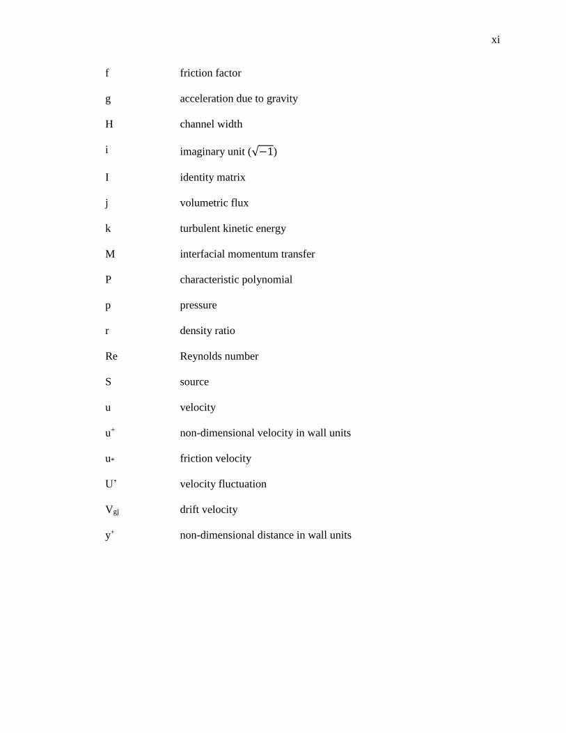
f friction factor
g acceleration due to gravity
H channel width
i imaginary unit (√−1)
I identity matrix
j volumetric flux
k turbulent kinetic energy
M interfacial momentum transfer
P characteristic polynomial
p pressure
r density ratio
Re Reynolds number
S source
u velocity
u+ non-dimensional velocity in wall units
u* friction velocity
U’ velocity fluctuation
Vgj drift velocity
y+ non-dimensional distance in wall units

xii
Greek
α void fraction
β two-phase friction velocity scaling factor
Δ filter size
ε turbulent eddy dissipation
κ von Karmann constant
λ eigenvalue
λk wave length
μ dynamic viscosity
ν kinematic viscosity
ρ density
σ surface tension
τ shear stress
ω growth rate
Superscripts
Coll collision
D drag
L lift
m mixture

xiii
n time level
T turbulent component
TD turbulent dispersion
VM virtual mass
W wall
x two-phase
Subscripts
b bubble
BI bubble induced
c cell center
CD central derivative
i interfacial
j junction
p peak
r relative
SI shear induced
UD upwind derivative
1,l liquid phase
2,g gas phase
∞ free stream
xiv
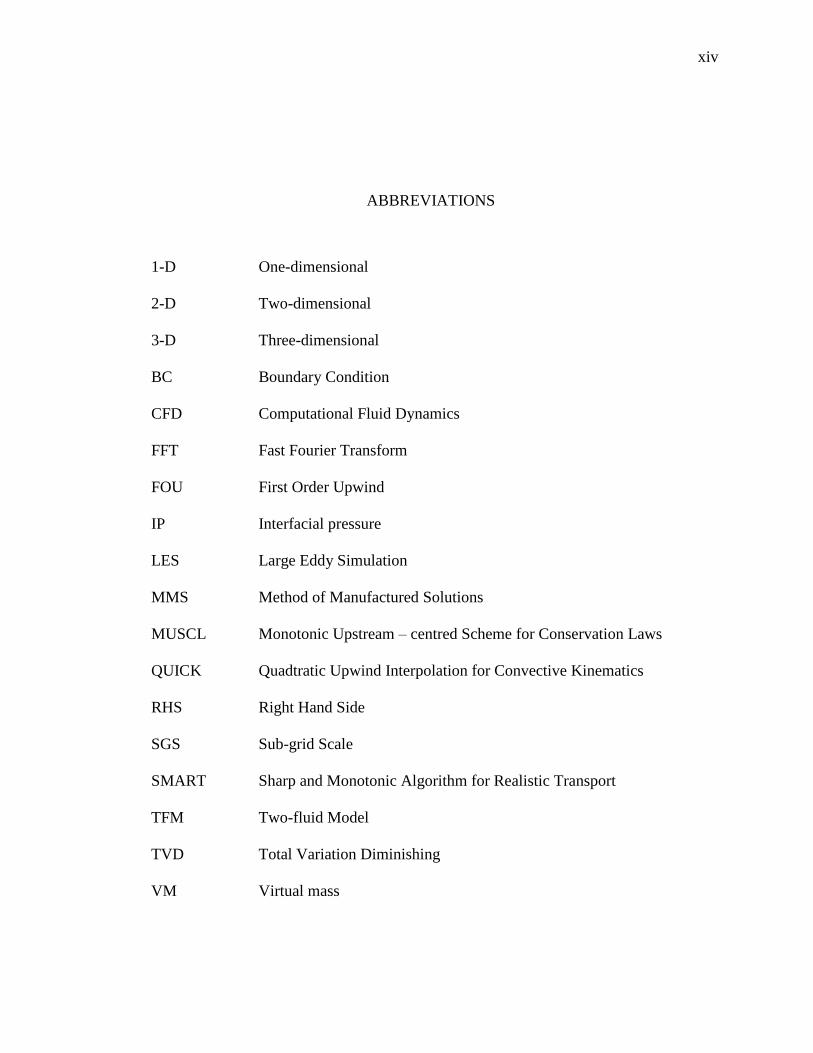
ABBREVIATIONS
1-D One-dimensional
2-D Two-dimensional
3-D Three-dimensional
BC Boundary Condition
CFD Computational Fluid Dynamics
FFT Fast Fourier Transform
FOU First Order Upwind
IP Interfacial pressure
LES Large Eddy Simulation
MMS Method of Manufactured Solutions
MUSCL Monotonic Upstream – centred Scheme for Conservation Laws
QUICK Quadtratic Upwind Interpolation for Convective Kinematics
RHS Right Hand Side
SGS Sub-grid Scale
SMART Sharp and Monotonic Algorithm for Realistic Transport
TFM Two-fluid Model
TVD Total Variation Diminishing
VM Virtual mass

xv
ABSTRACT
Vaidheeswaran, Avinash. Ph.D., Purdue University, May 2015.Well-posedness and
Convergence of CFD Two-fluid Model for Bubbly Flows. Major Professor: Martin Lopez
de Bertodano.
The current research is focused on developing a well-posed multidimensional CFD two-
fluid model (TFM) for bubbly flows. Two-phase flows exhibit a wide range of local flow
instabilities such as Kelvin-Helmholtz, Rayleigh-Taylor, plume and jet instabilities. They
arise due to the density difference and/or the relative velocity between the two phases. A
physically correct TFM is essential to model these instabilities. However, this is not the
case with the TFMs in numerical codes, which can be shown to have complex
eigenvalues due to incompleteness and hence are ill-posed as initial value problems. A
common approach to regularize an incomplete TFM is to add artificial physics or
numerically by using a coarse grid or first order methods. However, it eliminates the local
physical instabilities along with the undesired high frequency oscillations resulting from
the ill-posedness. Thus, the TFM loses the capability to predict the inherent local
dynamics of the two-phase flow. The alternative approach followed in the current study is
to introduce appropriate physical mechanisms that make the TFM well-posed.
First a well-posed 1-D TFM for vertical bubbly flows is analyzed with characteristics,
and dispersion analysis. When an incomplete TFM is used, it results in high frequency

xvi
oscillations in the solution. It is demonstrated through the travelling void wave problem
that, by adding the missing short wavelength physics to the numerical TFM, this can be
removed by making the model well-posed. To extend the limit of well-posedness beyond
the well-known TFM of Pauchon and Banerjee [1], the mechanism of collision is
considered, and it is shown by characteristics analysis that the TFM then becomes well-
posed for all void fractions of practical interest. The aforementioned ideas are then
extended to CFD TFM. The travelling void wave problem is again used to demonstrate
that by adding appropriate physics, the problem of ill-posedness is resolved.
Furthermore, issues pertaining to the presence of the wall boundaries need to be
addressed in a CFD TFM. A near-wall modeling technique is proposed which takes into
account the turbulent boundary conditions and void fraction distribution in the vicinity of
the wall. An important consequence of using the proposed technique is that the need of
wall force model, which is questionable when applied to air-water turbulent bubbly flows,
is eliminated. Also the bubbly TFM near the wall becomes convergent.
Finally, the well-posed CFD TFM developed in the present study is checked for grid
convergence. Previous researchers have advocated the idea of fixing the minimum grid
size based on bubble diameter. This has restricted a thorough verification exercise in the
past. It is shown that the grid size criterion can be removed if the model is made well-
posed, which also makes sense because a continuum model should be independent of grid
size. It is observed that the solution from the coarse grid simulations is a limit cycle
whereas upon grid refinement, the solution becomes chaotic which is characteristic of
xvii
turbulent bubbly two-phase flows. Therefore the grid size restriction may have an
unwanted consequence. FFT spectra and time averaged void fraction profiles are used to
assess grid convergence since the solutions are chaotic. The energy spectra indicate the
Kolmogorov -5/3 scaling commonly used to describe turbulent flows.

1
CHAPTER 1. INTRODUCTION
1.1 Significance of Problem
The research presented is focused on understanding the mathematical behavior of a CFD
TFM applied to vertical bubbly two-phase flows. Dispersed bubbly flows are of great
importance as they have desirable heat and mass transfer characteristics due to high
interfacial area concentration. In water cooled nuclear reactors, the bubbles nucleate from
the heated surface and migrate to the center thus providing an efficient channel for heat
transfer. In addition, bubbly two phase flows are relevant for safety aspects of nuclear
reactor operation. For example, in the passive cooling phase of a boiling water reactor
(BWR), the steam is vented into the suppression pool to remove the decay heat, resulting
in a two phase mixture flow. Also, it is important to understand the underlying physics of
the bubbly flows in order to model transient events leading to the critical heat flux in fuel
rod assemblies in reactors. Bubbly flows are also observed in a range of chemical
processes such as oxidation, alkylation, and chlorination. Other applications of bubbly
flows include stainless steel manufacturing, oil and gas industry and bioreactors.
CFD application for two-phase flows involves solving the TFM system of equations
derived from first principles as done by Ishii [2], and Vernier and Delhaye [3], and can be
applied to flows ranging from horizontal stratified flows to vertical annular flows. It is

2
hence important to understand the dominant mechanisms pertaining to specific flow
regimes. To make the TFM mathematically well-behaved, it is common to use an
artificial viscosity or a coarse grid to solve any issues that arise from an incomplete TFM.
Verification and validation exercises are a common practice in the field of numerical
modeling. If the TFM is ill-posed, it will not be possible to verify the model. It starts
showing non-physical behavior such as high frequency oscillations in the velocity and
void fraction distributions as the mesh is refined. The current research is directed at a
mechanistic approach to make the TFM well-posed. The important mechanisms
pertaining to the case of two-phase bubbly flows are identified, and eventually a well-
posed TFM is proposed that could be verified and validated.
1.2 Previous Work
Application of the TFM to analyze two-phase bubbly flows has been studied extensively
in the past by researchers. The well-posedness and stability of the TFM has always
remained a topic of debate. Ramshaw and Trapp [4] were among the first to analyze the
mathematical behavior of the TFM applied to stratified flows. It was recognized that by
adding appropriate physics to the TFM, it can be made well-posed. Lyczkowski et al. [5]
claimed that the TFM applied to bubbly flows is ill-posed as an initial value problem. It
was finally concluded that the TFM can be made well-posed if sufficient numerical
damping is added. Also, the eigenvalue analysis showed that the well-posedness was
dependent on parameters like pressure and liquid velocity. In practice, the well-posedness
of the TFM is determined by the eigenvalues associated with the material waves. They
must be real for the TFM to be well-posed regardless of the operating conditions. At this

3
point when there were different forms of TFM being proposed, certain aspects were still
being considered like, whether the void fraction should be included inside the pressure
gradient term. Lyczkowski et al. [5] proposed that the TFM becomes well-posed by doing
so. However, TFM derived rigorously from the first principles shows that the void
fraction term appears outside the pressure gradient term. Pauchon and Banerjee [1] were
the first to show the limit of TFM well-posedness in terms of non-dimensional
characteristics. This makes the well-posedness criterion independent of the conditions
like liquid velocity or pressure. Also, it was shown that the interfacial pressure force aids
in making the model well-posed while the behavior of the virtual mass force does the
opposite. This is in contradiction with the findings of Lyczkowski et al. [5] who
postulated that the virtual mass term increases the domain of well-posedness. Pauchon
and Banerjee [1] found that the interfacial pressure term proposed by Stuhmiller [6]
makes the TFM well-posed up to 26 % void fraction. Haley et al. [7] performed a
parametric study on the effect of interfacial pressure and the virtual mass coefficients on
the eigenvalues. The results obtained were consistent with the findings of Pauchon and
Banerjee [1]. Park et al. [8] derived a more complete TFM and performed a similar
parametric study and concluded that the region of well-posedness can be changed by
modifying these coefficients.
To extend the limit of well-posedness of the TFM applied to vertical bubbly flows, it is
shown here through the study of characteristics, that inter-bubble collisions need to be
considered. In the field of multiphase flows with particles, there are several models for
collision force. Ogawa et al. [9] were among the first to derive a constitutive relation for
4
momentum transfer due to collisions by using a simple binary collision model and
statistical averaging of the particle stress tensor. Savage and Jeffrey [10] developed a
mechanistic model for the particle collisions. The particles were assumed to have
velocities following a Maxwellian distribution. The spatial pair distribution function of
Carnahan and Starling [11] was used which was found to be in good agreement with the
molecular dynamics calculations up to a void fraction of 0.5. Lun et al. [12] followed a
similar procedure to that of Savage and Jeffrey [10] and extended their analysis to
inelastic collisions. Lun and Savage [13] proposed a modified correlation for the pair
distribution function and could be applied to the entire void fraction range observed for
particle flows. It behaves identical to that of Carnahan and Starling [11] for void fractions
up to 0.5. Beyond this limit, the correlation of Lun and Savage [13] follows the behavior
of the distribution function proposed by Ogawa et al. [9] which shows good agreement
with the molecular dynamics simulations for higher void fractions.
The TFM developed by Boelle et al. [14] includes the collisional contribution from direct
particle collisions and the turbulent motion of fluid and particles. The mechanism of
collision was seen to manifest itself as first and second order terms in the TFM, and the
model could be extended to inelastic collisions as well. The correlation proposed by Lun
and Savage [13] was used for the pair distribution function. Also, the contribution from
collisions was included in the governing equations for Reynolds stresses that provide
closure for turbulence modeling. Alajbegovic et al. [15] proposed a model for collision
force term derived by ensemble averaging the stress tensor using the pair correlation
function of Carnahan and Starling [11]. The model was validated with experiments of
Alajbegovic et al. [16] using ceramics, polystyrene and expanded polystyrene particles in

5
water covering a wide range of density ratios. Of particular interest is the case of
expanded polystyrene particles, where, the specific gravity (0.032) and particle diameter
(1.79 mm) are similar to the conditions of air-water two-phase flows.
The present research deals with the application of the well-posed TFM for the CFD
analysis of the bubble column experiments of Reddy Vanga [17]. There is a large body of
work concerning CFD simulations of dispersed bubbly flows using the Eulerian TFM.
One of the first numerical simulations on bubble columns was performed by Deen et al.
[18]. The results obtained with the LES and k-ε models were compared with the
experiments and it was concluded that the former shows better agreement. Lakehal et al.
[19] developed filtered TFM equations which are similar to the TFM of Ishii [2].In
addition, Lakehal et al. [19] proposed a filter size restriction that it should to be greater
than the bubble diameter. Milelli [20] proposed a criterion for the cut off filter size and
concluded that optimum results were obtained with a filter size to bubble diameter ratio
of 1.5. Zhang et al. [21] performed a sensitivity analysis of the coefficients for the TFM
closure relations including the sub-grid scale viscosity model of Smagorinsky [22], as
well as drag, lift and virtual mass forces. Dhotre et al. [23] performed CFD simulations of
a bubble column with LES using Smagorinsky [22] and dynamic Germano (1991) models.
It is found, in general, that a model constant of 0.1 for the model of Smagorinsky [22]
performs well in the case of two-phase bubbly flows. Niceno et al. [24] used a more
elaborate Eulerian TFM approach with LES, where a one-equation sub-grid scale model
for the kinetic energy is used. Recently, Ojima et al. [25] performed experiments and
numerical analysis of flow in a bubble column. They concluded that if the vortical
6
structures are predominant over the shear induced and bubble induced components of
turbulenc, the TFM gives reasonable predictions without the LES or RANS approach.
An important aspect of 3D TFM simulations is the near-wall treatment. Usually, the
boundary condition for the momentum equation is supplied through the standard
logarithmic law of the wall. In the presence of the bubbles, Marie et al. [26] observed that
the slope of the liquid velocity profile changes in the near-wall region. A mechanistic
model was proposed by Marie et al. [26] for the modified logarithmic law of the wall. It
was observed that the slope still remains constant, while the intercept changes based on
void fraction. In terms of near-wall modeling of the void fraction, it still remains to be
explained if conventional CFD TFM is the right approach. Larrateguy et al. [27], and
Moraga et al. [28] followed a different approach by introducing the bubble center
averaging methodology to separate the geometry of the bubbles from the force dynamics.
It is demonstrated here that by using, a well-posed CFD TFM, with the appropriate near-
wall modeling, reasonable convergence can be obtained, and that CFD calculations can
be performed with finer grid sizes (beyond the criterion set by Milelli [20]), which had
not been done in the past.
1.3 Thesis Outline
In the second chapter, the complete 3-D TFM of Ishii [2] for adiabatic two-phase flows is
described along with the constitutive relations. A brief account of 1-D TFM is given,
leading to the formulation of the fixed-flux 2-equation TFM, and drift flux void
propagation equation. In chapter 3, a detailed description of the eigenvalue analysis is

7
given. By adding the collision mechanism to the TFM, it is shown that the TFM becomes
well-posed in the domain of practical interest. In chapter 4, the non-linear void wave
propagation behavior of a stable kinematic wave is understood. Using a traveling void
wave problem, the issue of well-posedness is discussed. The fixed-flux 2-equation TFM,
and void propagation equation are solved numerically and it is shown that the results are
similar for a kinematically stable wave. Chapter 5 includes with the analysis and results
from CFD TFM calculations. As done in Chapter 4, the issue of ill-posedness is
demonstrated with a travelling void wave problem, which is shown to be removed by
adding appropriate physics. The near-wall modeling approach and its application to the
steady state two-phase flow conditions is discussed. Finally, the transient CFD
calculations of the bubble plume instability are analyzed, and it is shown with the FFT
spectra that the well-posed CFD TFM converges. Additionally, in Appendix A, the exact
analytical values of the characteristics are provided. In Appendix B, the collision force
model used in the present study is derived. Appendix C provides a comparison between
the acoustic roots predicted by the TFM with the experimental data. Further it is
demonstrated that the material wave propagation speeds are not affected by introducing
compressibility into the TFM. Finally, in Appendix D, the method of manufactured
solutions is discussed in the context of fixed-flux 2-equation TFM and CFD TFM, and it
is shown that the numerical schemes used in the present study are of higher order.

8
CHAPTER 2. TWO-FLUID MODEL
2.1 Governing equations
TFM describes the set of governing equations considering the constituent phases
separately each being characterized by an independent velocity field. Instead of analyzing
the local instant mass, momentum or energy transfer at the interface, collective
interactions are modeled in the TFM. Two-phase flows are observed to have quite a few
flow instabilities which arise due to difference in density and/or relative velocity between
the two phases. Since TFM allows each of the phases to have its own velocity field, it has
the capability to model flow dynamics driven by the relative velocity between the phases.
It is an important tool in analyzing transient phenomenon such as sudden mixing of
phases or flow regime transition where the two phases are weakly coupled. In comparison,
in the drift flux model introduced by Zuber and Findlay [29], the velocities of the
constituent phases are related to each other by the drift flux expressions depending on the
flow regime. Even though, the drift flux model is often considered reliable for flows that
are strongly coupled, it is not sufficient to transient phenomena.
In the current research, the adiabatic TFM applied to vertical bubbly two-phase flows is
considered following the work of Ishii [2]. The focus is on the hydrodynamics of the

9
constituent phases, and hence the energy equation will be neglected. The set of continuity
and momentum equations for each phase are given by,
𝜕
𝜕𝑡𝛼𝑘𝜌𝑘 + 𝛻. 𝛼𝑘𝜌𝑘��𝑘 = г𝑘 (2.1)
𝜕
𝜕𝑡𝛼𝑘𝜌𝑘��𝑘 + ∇. 𝛼𝑘𝜌𝑘��𝑘��𝑘
= −𝛼𝑘∇𝑝𝑘 + ∇. 𝛼𝑘(𝜏�� + 𝜏��𝑇) + 𝛼𝑘𝜌𝑘𝑔 + 𝑀𝑘𝑖
− (𝑝𝑘𝑖 − 𝑝𝑘)∇𝛼𝑘 + (𝜏��𝑖 − 𝜏��). ∇𝛼𝑘 + ��𝑘𝑖г𝑘
(2.2)
where k = 1 for liquid and k = 2 for gas phase. 𝛼𝑘, 𝜌𝑘, ��𝑘 are the void fraction, density
and velocity field corresponding to phase k. In addition, the void fraction of the phases
must satisfy the constraint,
∑ 𝛼𝑘
𝑘
= 1 (2.3)
Since the research presented here is restricted to the case of adiabatic flows, the inter-
phase mass transfer rate, г𝑘 = 0. Also, the momentum transfer due to mass transfer can be
neglected for the case of flows with no phase change. The term 𝑀𝑘𝑖 represents the
averaged contribution from the net momentum transfer occurring at the interface between
the two phases. It can be decomposed as shown below.
𝑀𝑘𝑖 = 𝑀𝑘𝑖𝐷 + 𝑀𝑘𝑖
𝐿 + 𝑀𝑘𝑖𝑇𝐷 + 𝑀𝑘𝑖
𝑊 + 𝑀𝑘𝑖𝑉𝑀 + 𝑀𝑘𝑖
𝐵 (2.4)
The terms on the RHS from left to right represent contributions from the drag, lift,
turbulent dispersion, wall, virtual mass and Basset forces respectively. For numerical
calculations, Basset force is usually neglected, since it is tough to compute the term

10
which involves integral over time. The terms 𝜏𝑘𝑖 and 𝑝𝑘𝑖 represent the shear stress and
the pressure at the interface respectively.
2.2 Constitutive Relations
2.2.1 Interphase momentum transfer
An essential part of the TFM is to account for the interactions between the constituent
phases. Since it is tough to physically account for the momentum transfer at each
interface, the averaged contribution is considered after time averaging the local instant
formulation (Ishii [2]). This couples the motion of the constituent phases, and determines
the phase distribution. It is important to note that the terms in Eq. (2.4) represent the
combined averaged effects of pressure and shear stress deviation from the mean value,
and not the absolute effect of the two. This distinction is important so that the relative
velocity or phase distribution is affected only by the flow dynamics and not by the
operating conditions. The macroscopic momentum jump condition is then given by,
∑ 𝑀𝑘𝑖
𝑘
= 0 (2.5)
This indicates the requirement that the forces acting at the interface form an action-
reaction pair for the constituent phases.
2.2.1.1 Drag
The momentum transfer due to drag force includes contributions from both the skin and
form drag under steady state conditions. The general form is given by,

11
𝑀2𝑖𝐷 = −
3
4𝛼2𝜌1
𝐶𝐷
𝐷𝑏
|��𝑟|��𝑟 (2.6)
The coefficient CD varies depending on the flow regime of the two-phase flows. For a
single particle, CD depends on the nature of the particle and the flow around it. For the
case of a multi-particle system, the presence of neighboring particles also affects the drag
coefficient. Following the work of Ishii and Chawla [30], the effect of surrounding
particles is taken into account through a mixture viscosity given by,
𝜇𝑚
𝜇1= (1 −
𝛼2
𝛼2𝑝)
−2.5𝛼2𝑝𝜇∗
(2.7)
where,
𝜇∗ =𝜇2 + 0.4𝜇1
𝜇2 + 𝜇1 (2.8)
The parameter 𝛼2𝑝 refers to the packing limit. For Stokes flow regime,
𝐶𝐷 =24
𝑅𝑒𝑏 (2.9)
where, Reb is defined based on the mixture viscosity as,
𝑅𝑒𝑏 =𝜌1𝐷𝑏𝑢𝑟
𝜇𝑚 (2.10)
For the case of distorted particles, the drag correlation is given by,
𝐶𝐷 =2
3𝐷𝑏√
𝑔Δ𝜌
𝜎(
1 + 17.67𝑓(𝛼2)6/7
18.67𝑓(𝛼2))
2
(2.11)
where,
𝑓(𝛼2) = (1 − 𝛼2)1.5 (2.12)
It can be seen from Eq. (2.11) that the drag coefficient increases with increasing particle
concentrations. For the CFD calculations reported in the present research, CD given by Eq.
(2.11) is used.
12
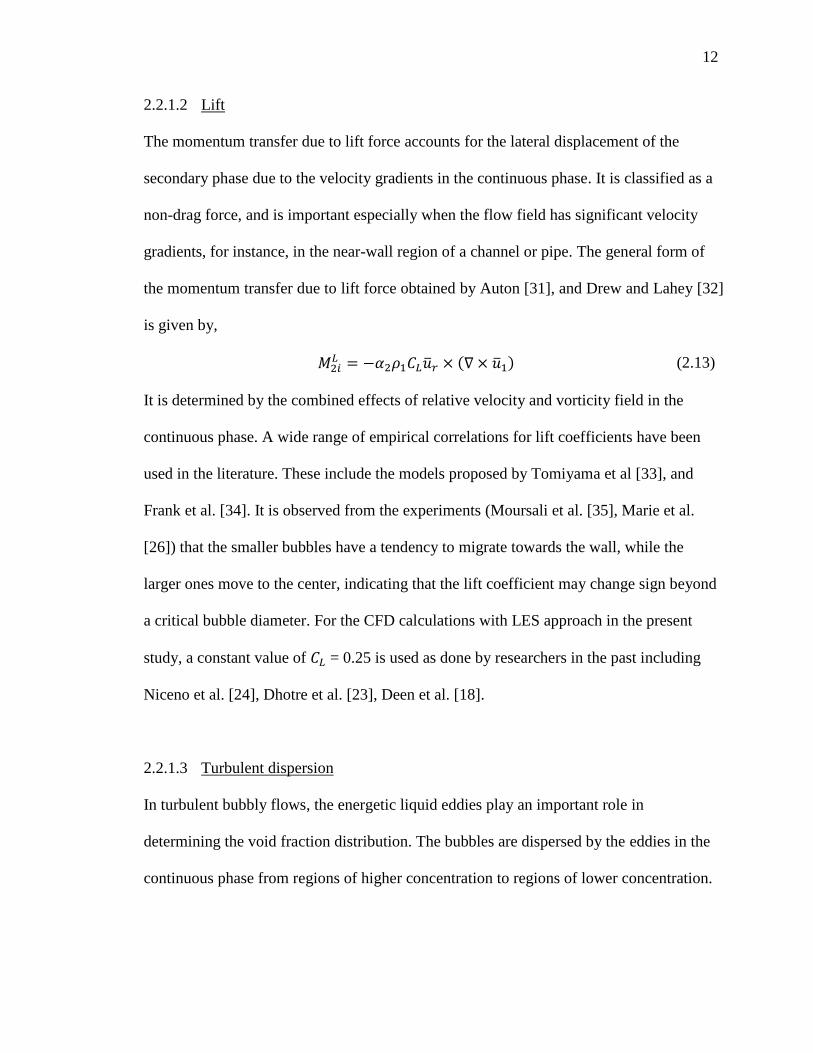
2.2.1.2 Lift
The momentum transfer due to lift force accounts for the lateral displacement of the
secondary phase due to the velocity gradients in the continuous phase. It is classified as a
non-drag force, and is important especially when the flow field has significant velocity
gradients, for instance, in the near-wall region of a channel or pipe. The general form of
the momentum transfer due to lift force obtained by Auton [31], and Drew and Lahey [32]
is given by,
𝑀2𝑖𝐿 = −𝛼2𝜌1𝐶𝐿��𝑟 × (∇ × ��1) (2.13)
It is determined by the combined effects of relative velocity and vorticity field in the
continuous phase. A wide range of empirical correlations for lift coefficients have been
used in the literature. These include the models proposed by Tomiyama et al [33], and
Frank et al. [34]. It is observed from the experiments (Moursali et al. [35], Marie et al.
[26]) that the smaller bubbles have a tendency to migrate towards the wall, while the
larger ones move to the center, indicating that the lift coefficient may change sign beyond
a critical bubble diameter. For the CFD calculations with LES approach in the present
study, a constant value of 𝐶𝐿 = 0.25 is used as done by researchers in the past including
Niceno et al. [24], Dhotre et al. [23], Deen et al. [18].
2.2.1.3 Turbulent dispersion
In turbulent bubbly flows, the energetic liquid eddies play an important role in
determining the void fraction distribution. The bubbles are dispersed by the eddies in the
continuous phase from regions of higher concentration to regions of lower concentration.

13
This phenomenon is represented in terms of an averaged momentum exchange term. The
turbulent dispersion force model developed by Lopez de Bertodano [36] is given by,
𝑀2𝑖𝑇𝐷 = −𝐶𝑇𝐷𝜌1𝑘1∇𝛼2 (2.14)
The momentum transfer due to turbulent dispersion is directly proportional to the
turbulent kinetic energy which gives a measure of the velocity fluctuations in the
continuous phase. A constant value of 𝐶𝑇𝐷=0.25 is used in the present study for steady
state CFD TFM calculations. For CFD calculations with LES, the eddy interactions with
the bubbles are resovled by using very fine grid, and hence a model for momentum
transfer due to turbulent dispersion is not required.
2.2.1.4 Wall
The presence of wall results in the difference in the rate at which the liquid flows around
the bubbles in the near-wall region. One side of the bubble experiences slower liquid
flow along the surface due to the no slip condition at the wall. This results in the
movement of the bubbles away from the wall. The model proposed by Antal et al. [37] is
most commonly used, given by,
𝑀2𝑖𝑊 = −𝛼2𝜌1𝐶𝑤𝑎𝑙𝑙|𝑢𝑟|2𝑛 (2.15)
𝐶𝑤𝑎𝑙𝑙 = 𝑚𝑖𝑛 {0, − (𝑐𝑤1
𝐷𝑏+
𝑐𝑤2
𝑦𝑤𝑎𝑙𝑙)} (2.16)
In addition, there exist models for wall force coefficient proposed by Tomiyama et al. [33]
and Frank et al. [34] based on the model of Antal et al. [37]. The most common approach
for the near-wall modeling in CFD is to use the wall force model given by Eq. (2.15) to
14
prevent non-physical void fractions in the near-wall region. The model of Antal et al. [37]
was calibrated based on the experiments of Nakoryakov, where perfectly spherical
bubbles having Db = 0.87 mm were generated and used for the experiments conducted at
low Re. In effect, the conditions were laminar given the small bubble size and low liquid
flow rates. The use of the same model for turbulent air-water bubbly flows is
questionable, where the flow rates are higher and the bubble sizes are larger. In the
present research, a new near-wall modeling procedure is proposed as explained in
Chapter 5.
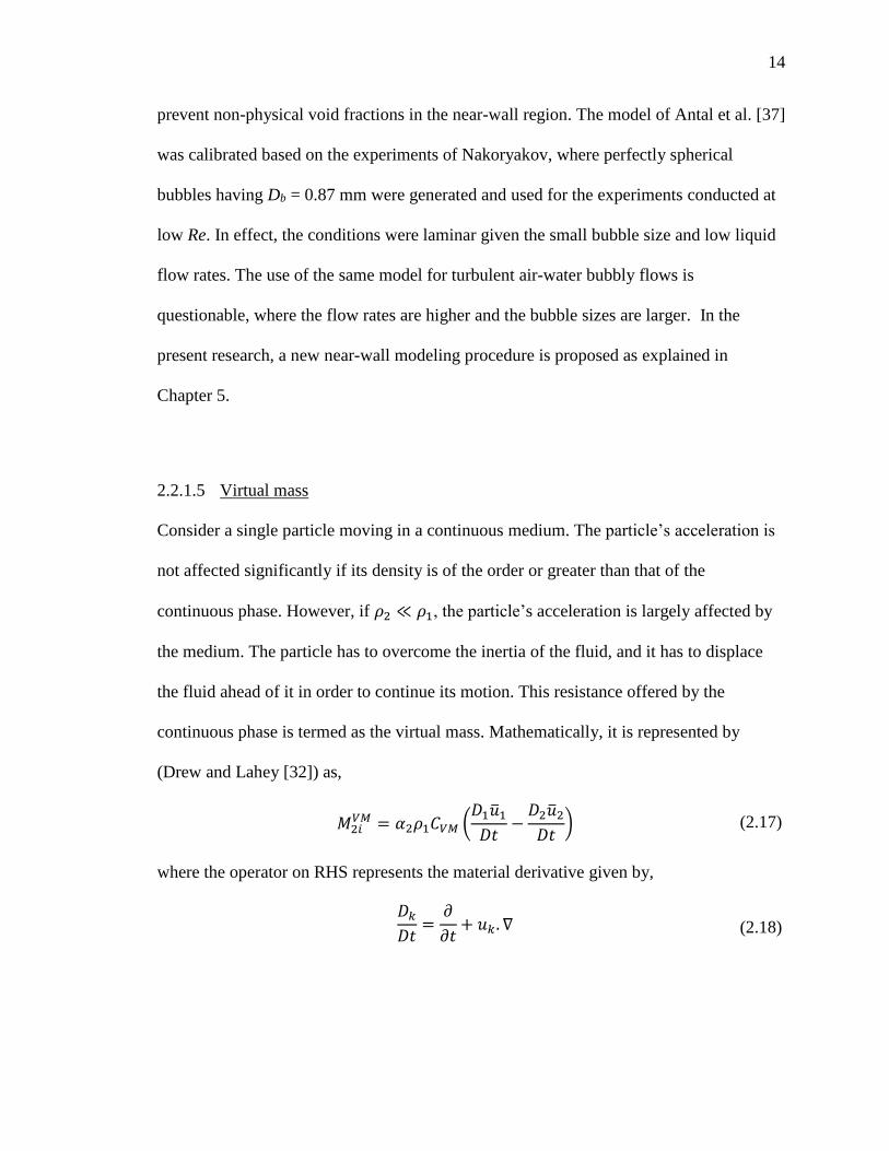
2.2.1.5 Virtual mass
Consider a single particle moving in a continuous medium. The particle’s acceleration is
not affected significantly if its density is of the order or greater than that of the
continuous phase. However, if 𝜌2 ≪ 𝜌1, the particle’s acceleration is largely affected by
the medium. The particle has to overcome the inertia of the fluid, and it has to displace
the fluid ahead of it in order to continue its motion. This resistance offered by the
continuous phase is termed as the virtual mass. Mathematically, it is represented by
(Drew and Lahey [32]) as,
𝑀2𝑖𝑉𝑀 = 𝛼2𝜌1𝐶𝑉𝑀 (
𝐷1��1
𝐷𝑡−
𝐷2��2
𝐷𝑡) (2.17)
where the operator on RHS represents the material derivative given by,
𝐷𝑘
𝐷𝑡=
𝜕
𝜕𝑡+ 𝑢𝑘 . ∇ (2.18)

15
For the case of potential flow around a sphere, CVM = 0.5 is used. For deformable bubbles,
correlations of Lamb [38] can be used. For higher concentrations, Zuber [39] developed a
correlation given by,
𝐶𝑉𝑀 =1
2(
1 + 2𝛼2
1 − 𝛼2) (2.19)
Physically, the virtual mass force is significant for the case of vertical bubbly flows.
When a bubble starts moving from rest under the action of buoyancy, it accelerates until
it reaches the terminal velocity, and the rate at which the velocity of the particle increases
is controlled by this transient term. In terms of the mathematical behavior of the TFM
system of equations, the characteristic roots or eigenvalues corresponding to the material
wave propagation is affected by the virtual mass term which consists of both the spatial
and temporal derivatives.
2.2.2 Interfacial pressure
Another factor that influences the phase distribution is the difference in pressure between
the interface and far-field. Following Bernoulli’s principle, for an inviscid flow past a
sphere, the difference between the interfacial pressure and the continuous phase pressure
is given by (Stuhmiller, [6]),
𝑝1𝑖 − 𝑝1 = −𝐶𝑝𝜌1|��𝑟|2 (2.20)
where, Cp = 0.25 is used which is obtained by evaluating the area average of the pressure
difference over the surface of a sphere. Pauchon and Banerjee [1] conclude that for
dispersed flow regime, the pressure in the dispersed phase is almost equal to the pressure
at the interface, and hence 𝑝2𝑖 ≈ 𝑝2. The interfacial pressure difference plays an

16
important role in regularizing the TFM applied to vertical bubbly flows. When this term
is not considered, the model is unconditionally ill-posed. It is shown by Pauchon and
Banerjee [1], Haley et al. [7], and Park et al. [8] that the TFM can be made well-posed by
using the interfacial pressure term given by Eq. (2.20). The effect of adding interfacial
pressure term to the TFM formulation will be discussed in detail in Chapter 3 using linear
stability analysis.
2.2.3 Turbulence
As for the single phase flows, the turbulence in the continuous phase needs to be closed
by using an appropriate model. The stress terms in the continuous phase appearing on the
right hand side of Eq. (2.2) can be represented as,
𝜏1 + 𝜏1𝑇 = 𝜌1 (𝜈1(∇��1 + ∇��1
+) − (2
3𝜈1 − 𝜆1) ∇. ��1𝐼) (2.21)
where, 𝜈1, and 𝜆1 are the effective kinematic viscosity of the continuous phase and the
bulk viscosity of the continuous phase respectively. For the two-phase bubbly flows, the
closure for the Reynolds stresses in Eq. (2.2) is based on the approach of Lopez de
Bertodano et al. [41]. This model assumes linear superposition of the shear induced and
bubble induced (pseudo turbulence) turbulent stresses. The effective viscosity is given by,
𝜈1 = 𝜈1,𝐿 + 𝜈1,𝑆𝐼𝑇 + 𝜈1,𝐵𝐼
𝑇 (2.22)
where, 𝜈1,𝐿, 𝜈1,𝑆𝐼𝑇 , and 𝜈1,𝐵𝐼
𝑇 represent the material viscosity of the liquid, shear induced
component of the eddy viscosity, and the bubble induced component of the eddy
viscosity respectively. The closure for the shear induced eddy viscosity is obtained from
the turbulence theory on single phase flows. The options available are algebraic models,

17
one-equation models, or two-equation models. For the two-equation k-epsilon model of
Launder and Spalding [42], the eddy viscosity is given by,
𝜈1,𝑆𝐼𝑇 = 𝐶𝜇
𝑘12
휀1 (2.23)
where, Cμ = 0.09.
For a more detailed turbulence modeling, the Reynolds stress transport equations are
used, where the individual stress components are solved using transport equations for
each one of them. For LES approach used in the present study, the closure provided by
the sub-grid scale viscosity model of Smagorinsky [22].is used which is given by,
𝜈1,𝑆𝐼𝑇 = (𝐶𝑠∆)2|𝑆1| (2.24)
where, Cs = 0.1. It accounts for the contributions from the turbulent eddies that are
smaller than the grid size, and that are not resolved by the CFD approach.
The relative motion of the dispersed phase in a continuous phase results in bubble
induced turbulence or pseudo-turbulence. The bubble induced viscosity following the
correlation of Sato and Sekoguchi [43] is given by,
𝜈1,𝐵𝐼𝑇 = 𝐶𝑆𝑎𝑡𝑜𝛼2𝐷𝑏|��𝑟| (2.25)
where,|��𝑟|and 𝐷𝑏 are the corresponding velocity and length scales to describe the motion
of bubbles in liquid. The value of CSato recommended by Sato and Sekoguchi [43] is 0.6.

18
2.3 1-D Two-Fluid Model
2.3.1 4-equation TFM
The 3-D TFM is very elaborate and is used to describe the detailed interaction
mechanisms of the constituent phases through the interfacial transfer terms occurring in
the conservation equations. This makes 3-D TFM important in describing transient
phenomenon such as flow-regime transition where the constituent phases may be weakly
coupled. If the problem being analyzed has significantly dominant features in the flow
direction alone compared to the transverse directions, a suitable alternative is to use 1-D
TFM derived from the 3-D TFM based on area averaging. It reduces the complexity of
developing a numerical code considerably. Also, the computational load for analysis is
less compared to using a 3-D TFM numerical code.
The 1-D TFM can be derived by area averaging the 3-D TFM described by Eqs. (2.1, 2.2).
Consider a channel or a pipe having a cross-sectional area A. The area averaged value of
an independent variable φ is given by,
⟨𝜙⟩ =1
𝐴∬ 𝜙 𝑑𝐴 (2.26)
The void-weighted mean value is given by,
⟨⟨𝜙⟩⟩ =⟨𝛼𝜙⟩
⟨𝛼⟩ (2.27)
The resulting set of equations after area averaging Eqs. (2.1, 2.2) given by Ishii and
Hibiki [44] are:
𝜕
𝜕𝑡⟨𝛼𝑘⟩𝜌𝑘 +
𝜕
𝜕𝑥⟨𝛼𝑘⟩𝜌𝑘⟨⟨𝑢𝑘⟩⟩ = ⟨г𝑘⟩ (2.28)

19
𝜕
𝜕𝑡⟨𝛼𝑘⟩𝜌𝑘⟨⟨𝑢𝑘⟩⟩ +
𝜕
𝜕𝑥𝐶𝑣𝑘⟨𝛼𝑘⟩𝜌𝑘⟨⟨𝑢𝑘⟩⟩2
= −⟨𝛼𝑘⟩𝜕
𝜕𝑥⟨⟨𝑝𝑘⟩⟩ +
𝜕
𝜕𝑥⟨𝛼𝑘⟩⟨⟨𝜏𝑘𝑧𝑧 + 𝜏𝑘𝑧𝑧
𝑇 ⟩⟩ −4𝛼𝑘𝑤𝜏𝑘𝑤
𝐷
− ⟨𝛼𝑘⟩𝜌𝑘𝑔𝑥 + ⟨𝑀𝑘⟩ − ⟨(𝑝𝑘𝑖 − 𝑝𝑘)𝜕𝛼𝑘
𝜕𝑥⟩ + ⟨г𝑘⟩⟨⟨𝑢𝑘𝑖⟩⟩
(2.29)
where, ⟨𝑀𝑘𝑑⟩ represents the total interfacial shear force given by,
⟨𝑀𝑘⟩ = ⟨𝑀𝑘𝑖 − ∇𝛼𝑘. 𝜏𝑖⟩𝑧 (2.30)
The term 𝑀𝑘𝑖 represents contributions from drag, and virtual mass forces. The lift force is
not included since the equations are area averaged. From here on for simplicity, the
operators, < >, << >> are dropped. The covariance term 𝐶𝑣𝑘 is given by Ishii and Hibiki
[44] as,
𝐶𝑣𝑔 ≈ 1 + 0.5(𝐶0 − 1) (2.31)
𝐶𝑣𝑓 ≈ 1 + 1.5(𝐶0 − 1) (2.32)
where, 𝐶0 is the distribution parameter which is defined as,
𝐶0 =⟨𝛼2𝑗⟩
⟨𝛼2⟩⟨𝑗⟩ (2.33)
For the case of short wavelength instabilities studied here, it is assumed the void fraction
and the liquid velocity distributions are uniform in the lateral directions. Hence, 𝐶0 = 1 is
used and hence, 𝐶𝑣𝑓 , 𝐶𝑣𝑔 = 1 . In addition, if the incompressibility and isothermal flow

20
assumptions are made, and the wall friction is dropped, Eq. 2.27, and Eq. 2.28 can be
simplified as,
𝜕𝛼1
𝜕𝑡+
𝜕
𝜕𝑥𝛼1𝑢1 = 0 (2.34)
𝜕𝛼2
𝜕𝑡+
𝜕
𝜕𝑥𝛼2𝑢2 = 0 (2.35)
𝜌1𝛼1 (𝜕𝑢1
𝜕𝑡+ 𝑢1
𝜕𝑢1
𝜕𝑥)
= −𝛼1
𝜕𝑝1
𝜕𝑥+
𝜕
𝜕𝑥𝛼1(𝜏𝑘𝑧𝑧 + 𝜏𝑘𝑧𝑧
𝑇 ) − 𝛼1𝜌1𝑔𝑥 − 𝑀2𝑖𝑉𝑀 − 𝑀2𝑖
𝐷
− (𝑝1𝑖 − 𝑝1)𝜕𝛼1
𝜕𝑥
(2.36)
𝜌2𝛼2 (𝜕𝑢2
𝜕𝑡+ 𝑢2
𝜕𝑢2
𝜕𝑥) = −𝛼2
𝜕𝑝1𝑖
𝜕𝑥− 𝛼2𝜌2𝑔𝑥 + 𝑀2𝑖
𝑉𝑀 + 𝑀2𝑖𝐷 (2.37)
It must be noted that the area averaged momentum transfer due to drag force should be
dependent on the averaged local slip velocity ⟨𝑢𝑟⟩, and not the difference between the
area averaged mean velocities, ��𝑟 = ⟨⟨𝑢2⟩⟩ − ⟨⟨𝑢1⟩⟩. ��𝑟 includes contributions from local
relative motion and the global profile effect of void fraction and velocities. Hence, using
this value in general may lead to inaccurate results. To use ⟨𝑢𝑟⟩ in the drag force
formulation, the correlation proposed by Ishii and Hibiki [44] can be used,
⟨𝑢𝑟⟩ ≈1 − 𝐶0⟨𝛼2⟩
1 − ⟨𝛼2⟩⟨⟨𝑢2⟩⟩ − 𝐶0⟨⟨𝑢1⟩⟩ (2.38)

21
However, in the present study, the focus is on analyzing short wavelength physics, and
the profile effects are neglected and the value of 𝐶0 = 1 is used, resulting in ⟨𝑢𝑟⟩ ≈ ��𝑟
2.3.2 Fixed-flux 2-equation TFM
The 4 Equation TFM for incompressible two-phase bubbly flows described by Eq. (2.34)
– Eq. (2.37) forms the basis for deriving the fixed-flux 2-equation TFM. The following
assumptions are made to obtain the final set of PDEs:
very low density ratio, 𝜌2 𝜌1⁄ ≪ 1
constant volumetric flux, 𝑗 = 𝐶
While making these assumptions, the focus shifts to the short wavelength behavior of the
TFM. In particular, it is suitable to analyze adiabatic air-water systems which satisfy the
aforementioned assumptions. An important limitation of this model however is that the
system or integral instabilities like the density wave oscillations cannot be analyzed. The
steps used to obtain the 2 Equation TFM as shown in Lopez de Bertodano et al. [45] is
outlined as follows. The first PDE is the sum of two continuity equations (Eqs. 2.34, 2.35)
given by,
𝜕
𝜕𝑡(𝜌1𝛼1 + 𝜌2𝛼2) +
𝜕
𝜕𝑥(𝜌1𝛼1𝑢1 + 𝜌2𝛼2𝑢2) = 0 (2.39)
The second PDE is obtained from the difference in the momentum equations (Eqs. 2.36,
2.37), after dividing them by the respective volume fractions, where the pressure gradient
term gets eliminated. It is given by,

22
(1 +𝐶𝑉𝑀
𝛼1)
𝐷1
𝐷𝑡𝜌1𝑢1 − (1 +
𝐶𝑉𝑀
𝑟 𝛼1)
𝐷2
𝐷𝑡𝜌2𝑢2 +
𝜕
𝜕𝑥𝐶𝑝𝜌1(𝑢2 − 𝑢1)2
+𝐶𝑝
𝛼1𝜌1(𝑢2 − 𝑢1)2
𝜕𝛼1
𝜕𝑥
= −(𝜌1 − 𝜌2)𝑔 −2
𝛼1𝐻
𝑓1
2𝜌1𝑢1
2 + (1
𝛼1+
1
𝛼2) 𝑀2𝑖
𝐷
(2.40)
where, 𝑟 = 𝜌2 𝜌1⁄ The constraints applied to these two equations are the void fraction
and volumetric flux conditions given by,
𝛼1 + 𝛼2 = 1 (2.41)
and,
𝛼1𝑢1 + 𝛼2𝑢2 = 𝑗 (2.42)
The two equations (Eqs. 2.39, 2.40) are recast as follows,
𝑑
𝑑𝑡𝜓 +
𝑑
𝑑𝑥𝜑 = 𝜍 (2.43)
where,
𝜓 = [
𝜌1𝛼1 + 𝜌2𝛼2
(1 + 𝑏)𝜌1𝑢1 − (1 +𝑏
𝑟) 𝜌2𝑢2
], (2.44)
𝜑 = [
𝜌1𝛼1𝑢1 + 𝜌2𝛼2𝑢2
1
2(1 + 𝐶𝑉𝑀/𝛼1)𝜌1𝑢1
2 −1
2(1 +
𝐶𝑉𝑀
𝑟𝛼1)𝜌2𝑢2
2 + 𝐶𝑝𝜌1(𝑢2 − 𝑢1)2] (2.45)
RHS of Eq. (2.43) represents the source terms given by,
𝜍 = [
0
−(𝜌1 − 𝜌2)𝑔 −2
𝛼1𝐻
𝑓1
2𝜌1|𝑢1|𝑢1 + 𝑀2𝑖
𝐷 ] (2.46)

23
The final step is to convert Eq. (2.43) into governing equations for primitive variables
given by,
𝐴𝜕
𝜕𝑡𝜙 + 𝐵
𝜕
𝜕𝑥𝜙 = 𝐹 (2.47)
where, 𝜙 = [𝛼1 𝑢1]𝑇, and 𝐴 = 𝐼. The coefficient matrix B is obtained by simplification
based on Taylor series expansion about the parameter r, for r << 1, which is the case for
air-water flows. It is given by,
𝐵 ≅ [
𝑢1 𝛼1
(1 + 𝛼1)𝐶𝑝 − 𝐶𝑉𝑀
𝐶𝑉𝑀 + 𝛼1 − 𝛼12
(𝑢2 − 𝑢1)2 𝑢1 +2𝛼1(𝐶𝑉𝑀 − 𝐶𝑝)
𝐶𝑉𝑀 + 𝛼1 − 𝛼12
(𝑢2 − 𝑢1)] (2.48)
The source terms are given by,
𝐹 ≅𝛼1𝛼2
𝐶𝑉𝑀 + 𝛼1𝛼2[
0
−𝑔 −2
𝛼1𝐻
𝑓1
2|𝑢1|𝑢1 + (
1
𝛼1+
1
𝛼2)
𝑀2𝐷
𝜌1
] (2.49)
The final form of 2-equation TFM is given by,
𝜕𝛼1
𝜕𝑡+ 𝑢1
𝜕𝛼1
𝜕𝑥+ 𝛼1
𝜕𝑢1
𝜕𝑥= 0 (2.50)
𝜕𝑢1
𝜕𝑡+ 𝐵21
𝜕𝛼1
𝜕𝑥+ 𝐵22
𝜕𝑢1
𝜕𝑥
=𝛼1𝛼2
𝐶𝑉𝑀 + 𝛼1𝛼2[−𝑔 −
2
𝛼1𝐻
𝑓1
2|𝑢1|𝑢1 + (
1
𝛼1+
1
𝛼2)
𝑀2𝑖𝐷
𝜌1]
(2.51)
where,
𝐵21 =(1 + 𝛼1)𝐶𝑝 − 𝐶𝑉𝑀
𝐶𝑉𝑀 + 𝛼1𝛼2
(𝑢2 − 𝑢1)2 (2.52)

24
𝐵22 = 𝑢1 +2𝛼1(𝐶𝑉𝑀 − 𝐶𝑝)
𝐶𝑉𝑀 + 𝛼1𝛼2
(𝑢2 − 𝑢1) (2.53)
It can be seen that the resulting equations bear resemblance to the shallow water theory
equations (Whitham [46]) but for the convective part of Eq. (2.51). The advantage of
using such a model is that the computational load is reduced even further, and the
implementation of algorithm to solve the governing equations becomes straightforward.
It can be verified that the 2 equation TFM described above is similar to the model derived
by Haley et al. [7].
2.3.3 Drift flux void propagation equation
A further reduction of the 1D TFM can be made to obtain a one equation drift flux void
propagation equation model as follows. The drift flux model of Zuber and Findlay [29] is
given by,
⟨𝑗2⟩ = ⟨𝛼2𝑗⟩ + ⟨𝛼2𝑉𝑔𝑗⟩ (2.54)
which can be rewritten as,
𝑢2 = 𝐶0𝑗 + 𝑉𝑔𝑗 (2.55)
where, the operators have been dropped for simplicity. j follows the definition of Eq.
(2.42). Inserting Eq. (2.55) in the gas phase continuity equation (Eq. 2.56), the drift flux
void propagation equation can be obtained as,
𝜕𝛼2
𝜕𝑡+ (𝐶0𝑗 + 𝑉𝑔𝑗 + 𝛼2
𝑑𝑉𝑔𝑗
𝑑𝛼2)
𝜕𝛼2
𝜕𝑥= 0 (2.56)
where the drift velocity (Ishii and Chawla [30]) is given by,
𝑉𝑔𝑗 = √2 (𝜎𝑔∆𝜌
𝜌12 )
1/4
(1 − 𝛼2)1.75 (2.57)

25
Thus, the TFM is reduced to a single first order partial differential equation. The velocity
of propagation of the kinematic void wave is given by,
𝐶𝑘 = 𝐶0𝑗 + 𝑉𝑔𝑗 + 𝛼2
𝑑𝑉𝑔𝑗
𝑑𝛼2 (2.58)
It can be seen that Ck is only dependent on α2. Eq. (2.56) is always stable, as it eliminates
the local physical instabilities that arise due to the relative velocity between the two-
phases. However, the non-linear void wave propagation characteristics are retained as
indicated by numerical calculations in the Section 4. When the material wave stability
conditions are satisfied, the 1-D 4-equation TFM, the 2 equation TFM, and the drift flux
void propagation equation are expected to give identical solutions.

26
CHAPTER 3. LINEAR STABILITY ANALYSIS
3.1 Overview
The TFM of Ishii [2] is very elaborate as it is applicable to all the two-phase flow
regimes having different flow configurations. It is shown in Ishii and Hibiki [44] that the
total number of unknowns involved in the rigorous TFM formulation of Ishii [2] can be
as high as 33. To use the TFM for two-phase flow analysis, there is always a need to
simplify the model so that it can be implemented into an algorithm. Usually, in this
process, there is a tendency to neglect terms that may seem cumbersome depending on
the flow regime of interest. If even one of the terms being dropped is of physical
significance, then the TFM may be rendered ill-posed due to incompleteness. According
to Hadamard’s classical definition, a system is defined as well-posed if,
there exists a solution
the solution is unique
the solution depends continuously on data and parameters
It is important for the system to be well-posed, so that a physically meaningful solution is
obtained. To regularize the TFM in the present study, it is important to understand the
physics the two-phase vertical bubbly flows. Matuszkiewicz [47] performed experiments
to understand the flow pattern transition from bubbly to slug, where the instabilities of
the void fraction waves were studied. Park et al. [48] measured void wave propagation
27
speeds associated with dispersed and clustered bubbles in air-oil mixture to describe the
flow regime transition. Cheng et al. [49] analysed the effect of parameters such as bubble
diameter, superficial velocities on the instability of void fraction waves leading to
changes in flow regime from bubbly to slug flow having intermediate stages such as
bubble cluster and cap bubbly flows. Hence, we may expect the TFM applied to bubbly
flows to be hyperbolic in nature in order to represent the wave like behaviour observed in
reality.
Before the TFM is applied to analyse two-phase flows, it is important to check if the
system of equations is indeed hyperbolic. If the eigenvalues associated with the material
waves are real, the system is considered hyperbolic and thus well-posed as an initial
value problem as discussed by Pauchon and Banerjee [1], Haley et al. [7], and Park et al.
[8]. If the material waves have complex eigenvalues, then the system becomes elliptic,
and hence ill-posed. Mathematically it would imply that the current state depends on
future state which makes no physical sense. In determining the well-posedness of the
system, the acoustic roots are not considered, since they are always real. This is one of
the major reasons for using incompressible TFM to perform linear stability analysis. It
will be shown in Appendix C that the material wave characteristics remain unchanged
with the incompressibility assumption.
One of the methods to resolve TFM ill-posedness is to add excess viscosity, which
regularizes the TFM artificially. Another common approach is to use a coarse grid or first
order numerics or a combination of both to achieve numerical regularization. The

28
additional damping provided by discretization or numerical schemes removes high
frequency oscillations that may arise in the solution due to ill-posedness, and makes the
model appear well-behaved. An important consequence of such techniques is that the
physical flow instabilities are also damped. Owing to the density difference and relative
velocity between the constituent phases, two-phase flows are associated with a variety of
flow dynamics such as Kelvin-Helmholtz, Rayleigh-Taylor, jet and plume instabilities. A
physically correct TFM should be capable of modelling these instabilities, and at the
same time be well-posed. The over-stabilization achieved by numerical or artificial
regularization will result in physically incorrect solutions. The objective here is to
achieve regularization by adding terms that are motivated by the physics of the problem.
As a result, the TFM may be made well-posed, and it may also be capable of predicting
the flow instabilities.
3.2 Characteristics Analysis
The analysis of eigenvalues of a system of equations give an understanding of the
mathematical behaviour. As mentioned before, depending on the nature of the
characteristic roots, the TFM system can be classified as either well-posed or ill-posed.
For the case of TFM for vertical bubbly flows, Pauchon and Banerjee [1] were the first to
apply this idea in the context of TFM for vertical bubbly flows. They showed the
importance of considering interfacial pressure term and virtual mass terms to determine
the region of well-posedness. Haley et al. [7] performed a more detailed analysis by
including the effect of bubble induced turbulence in the TFM, and obtained results
similar to that of Pauchon and Banerjee [1]. Park et al. [8] obtained results similar to

29
Pauchon and Banerjee [1] as well, and were able to show that depending on the
coefficient values (virtual mass, and interfacial pressure) used in the TFM, the region of
well-posedness can be changed. To perform linear stability analysis on TFM, the system
of equations (Eq. (2.34) – (2.37)) is recast into the following form,
𝐴𝜕
𝜕𝑡𝜙 + 𝐵
𝜕
𝜕𝑥𝜙 + 𝐷
𝜕2
𝜕𝑥2𝜙 + 𝐹 = 0 (3.1)
where, 𝜙 = [𝛼2 𝑢2 𝑢1 𝑝 ]𝑇. The matrices A, B, D, and F are given in Appendix A. As
shown by Pauchon and Banerjee [1], the nature of evolution of the solution from an
initial condition can be understood by solving,
Det(𝐴𝜆 − 𝐵) = 0 (3.2)
This results in 4 eigenvalues, 2 of which correspond to acoustic waves and the remaining
2 correspond to the material waves whose exact mathematical forms are given in
Appendix A. The acoustic wave speeds are always real. It is the material wave speeds
which determine the well-posedness of the TFM under consideration. Pauchon and
Banerjee [1] define the parameter 𝜆∗ as,
𝜆∗ =𝜆 − 𝑢1
𝑢2 − 𝑢1 (3.3)
so that the dimensionless eigenvalue depends only on 𝛼2. In addition, it is shown by
Pauchon and Banerjee [1] that it is along 𝜆∗ given by Eq. (3.3) that the quantity conserved
can be closely approximated to 𝛼2. Hence 𝜆∗ is used to represent the TFM characteristic
roots in this section. The parameters listed in Table 3.1 are used for linear stability
analysis.

30
Table 3.1: Parameters for linear stability analysis
Parameter Value
ρ1 1000 kg/m3
ρ2 1 kg/m3
u1 0 m/s
u2 0.2 m/s
ν1 10-6 m2/s
ν2 1.56 x 10⁻⁵ m2/s
As seen in Fig. 3.1, the TFM for vertical bubbly flows with the interfacial pressure and
the virtual mass terms where, 𝐶𝑝 = 0.25, 𝐶𝑉𝑀 = 0.5 is well-posed up to a void fraction
limit of 26 %. This result is in accordance with the work of Pauchon and Banerjee [1],
Haley et al. [7], and Park et al. [8]. The conclusion made by the some of the previous
researchers was that the transformation of eigenvalues from being real to imaginary may
be attributed to flow regime transition. This is questionable since the effect of flow
regime transition may be expected at longer wavelengths. Characteristics analysis
pertains to the study of short wavelength physics in the limit of 𝜆𝑘 → 0, where the system
is always expected to have real eigenvalues. Also, physically, it is possible to have two-
phase flows with 𝛼2 > 0.26, where the TFM should ideally be hyperbolic. Even for the
low superficial gas velocities, it can be seen that, the local void fraction is higher locally
near the entrance region where the gas is injected. It is important that the TFM be made
well-posed for such cases.

31
Figure 3.1: Non-dimensional eigenvalues with CP=0.25, CVM=0.5
3.3 Collision mechanism
To overcome the issue of conditional well-posedness, the mechanism of collision is
considered. It has been observed experimentally (like Zaruba et al. [50]), that at regions
of higher void fractions, the bubbles have a greater tendency to collide, being closely
packed. It is hence important to consider this phenomenon to make the TFM more
complete. In the field of fluid-particle flows, there exist several models to account for this
effect. Chapman and Cowling [51] were among the first to derive an expression for the
collision force starting from Boltzmann transport equations. The collision integral that
appears on the right hand side is evaluated using a small deviation from the equilibrium
velocity distribution function. An important parameter to be considered in case of inter-
particle collisions is the pair distribution function 𝑔(𝛼2). Physically, it accounts for the

32
increase in collision frequency at higher concentrations. Ogawa et al. [9] considered shear
driven granular flows. A distribution function was proposed conceptually based on
packing fraction limit 𝛼𝑝 as,
𝑔(𝛼2) = (1 −𝛼2
𝛼𝑝)
−1/3
(3.4)
Lun and Savage [13] found this to be appropriate for flows with void fractions close to
the fully packed state through molecular dynamics calculations. . Another commonly
used pair distribution function correlation was proposed by Carnahan and Starling [11]
given by,
𝑔(𝛼2) =2 − 𝛼2
2(1 − 𝛼2)3 (3.5)
Lun and Savage [13] concluded that this expression was in good agreement with the
molecular dynamics calculations for flows up to 𝛼2 = 0.5. Lun and Savage [13] also
proposed an empirical correlation that may be appropriate for the entire range of void
fraction (upto the packing limit) given by,
𝑔(𝛼2) = (1 −𝛼2
𝛼𝑝)
−2.5𝛼𝑝
(3.6)
In the present research, the collision force model of Alajbegovic et al. [15] is used which
has been validated for vertical two-phase flows having density ratio and particle size
similar to that of air-water flows. The expression is given by,
𝑀𝑐𝑜𝑙𝑙 = −∇. [(𝜌2 + 𝜌1𝐶𝑉𝑀)𝑔(𝛼2)𝛼22(2𝑢2
′ 𝑢2′ + 𝑢2
′ . 𝑢2′ 𝐼)] (3.7)
The pair distribution function of Carnahan and Starling [11] given by Eq. (3.5) is used in
Eq. (3.7). The variation of 𝑔(𝛼2) as a function of 𝛼2 is shown in Fig. 3.2. It can be seen
that, as the concentration increases, the pair distribution function starts becoming more

33
Figure 3.2: Variation of g(α2)
and more dominant, and its effect cannot be neglected in regions of higher 𝛼2. It is
important to note that the contribution from the inter-bubble collisions is to be considered
only in the momentum equation for the gas phase, and not as an action-reaction force pair
between the gas and liquid phases.
The collision force model given by Eq. (3.7) is adapted for the present study. The particle
stress tensor is assumed to be istotropic. For the case of 1-D analysis, as shown in
Appendix B, the model reduces to,
𝑀𝑐𝑜𝑙𝑙 = −𝐶𝑐𝑜𝑙𝑙𝜌1𝐶𝑉𝑀2 ((3𝛼2
2𝑢𝑟2𝑔(𝛼2)
𝑑𝛼2
𝑑𝛼2+ 𝛼2
3𝑢𝑟2
𝑑𝑔(𝛼2)
𝑑𝛼2)
𝜕𝛼2
𝜕𝑥
+ 2𝛼23𝑢𝑟𝑔(𝛼2)
𝜕𝑢𝑟
𝜕𝑥)
(3.8)

34
When Eq. (3.8) is used in the characteristics analysis, it can be seen (Fig. 3.3) that the
TFM is made well-posed even beyond 𝛼2 = 0.26 , which was the limiting void fraction
as found by Pauchon and Banerjee [1]. This is a significant improvement over the
existing TFMs. Having made the TFM unconditionally well-posed, the analysis of bubbly
flows can be extended to understand the dynamics of phenomenon such as clustering or
flow regime transition that usually occur at higher gas phase concentrations.
Fig. 3.4 shows the comparison of non-dimensional eigenvalues with the data of Kytoma
and Brennen [52]. The faster of the two characteristics is alone compared, since it is
associated with the only material wave that is observed in the experiments. It will be
shown by dispersion analysis that the slower characteristic root is associated with
significant physical damping, because of which one may not see this in reality. It can be
seen in Fig. 3.4 that by using a suitable coefficient, 𝐶𝑐𝑜𝑙𝑙, the predictions are in good
agreement with the data of Kytomaa and Brennen [52]. The effect of compressibility on
the characteristics is discussed in Appendix C.

35
Figure 3.3: Non-dimensional eigenvalues with collision

36
Figure 3.4: Comparison with the data of Kytomaa and Brennan [50]
37
3.4 Dispersion analysis
The eigenvalue analysis gives information about the behaviour of a system of equations
in the limit of 𝜆𝑘 → 0. To understand the behavior of all the different wavelengths,
perturbation analysis is used, which is also referred to as the dispersion analysis. For the
case of horizontal stratified two-phase flows, Ramshaw and Trapp [4] and Pokharna et al.
[53] have used this method to study the well-posedness and instability of the TFM. In the
present study, it is used to discuss the well-posedness of the TFM applied to vertical
bubbly flows. The dispersion relation is obtained as follows. Each independent variable
of 𝜙 is perturbed about an initial reference state as,
𝜙 = 𝜙0 + 𝛿𝜙 (3.9)
When Eq. (2.34) – Eq. (2.37) are linearized using Eq. (3.9), the perturbed system of
equations can be recast into
𝐴𝜕
𝜕𝑡𝛿𝜙 + 𝐵
𝜕
𝜕𝑥𝛿𝜙 + 𝐷
𝜕2
𝜕𝑥2𝛿𝜙 +
𝜕𝐹
𝜕𝜙𝛿𝜙 = 0 (3.10)
An assumption is made that the reference state is steady with respect to the perturbations.
It can also be viewed as follows: the time and length scales associated with the
perturbations are much smaller than those characterizing the reference state (Pokharna et
al. [53]). The perturbation is assumed to take the form of a travelling wave given by,
𝛿𝜙 = 𝛿𝜙0𝑒𝑖(𝑘𝑥−𝜔𝑡) (3.11)
Using Eq. (3.11), Eq. (3.10) reduces to,
[−𝑖𝜔𝐴 + 𝑖𝑘𝐵 + (𝑖𝑘)2𝐷 +𝜕𝐹
𝜕𝜙] 𝛿𝜙 = 0 (3.12)
For a non-trivial solution 𝛿𝜙 to exist, the following relationship must be satisfied,

38
det [𝜔𝐴 − 𝑘𝐵 − 𝑖𝑘2𝐷 +𝜕𝐹
𝜕𝜙] 𝛿𝜙 = 0 (3.13)
The solution to Eq. (3.13) gives the dispersion relation. For the parameters listed in Table
(3.1), when 𝐶𝑝 = 0, 𝐶𝑉𝑀 = 0, it can be seen that the imaginary part of the angular
frequency 𝜔, is positive for 𝛼2 = 0.1. Further, as 𝜆𝑘 → 0, 𝜔 → ∞. This is an indicator
that the TFM is ill-posed and it is shown in Fig. 3.5. When viscous stresses are added to
the TFM for both the phases, it can be seen that the wave growth becomes bounded as
𝜆𝑘 → 0. This is an improvement over the basic model, however it is not sufficient.
Though the model is well-posed, it is highly unstable at very low 𝜆𝑘. Finally, when the
appropriate physics are added to the TFM, the growth is bounded as 𝜆𝑘 → 0 having a
negligible growth rate comparatively. This indicates a physically acceptable well-posed
behavior which is the case for 𝛼2 = 0.1 as seen in the experiments, where one may
observe dispersed bubbly flows. Fig 3.6 shows the dispersion relation for both the
material waves. It is evident that the growth rate associated with the slower characteristic
root is considerably less (highly negative). This may be the reason why only one of the
two waves are observed in the experiments which is not as highly damped as the other
one.
Finally, the effect of adding collision mechanism is considered at 𝛼2 = 0.3. It can be seen
in Fig. 3.7 that when the interfacial pressure and virtual mass terms alone are included in
the analysis, an ill-posed behavior is observed. When the momentum transfer due to
collision is added to the TFM, the growth rate is bounded as shown. It may be possible in
future to study transient phenomenon such as flow regime transition, or wave instability,

39
Figure 3.5: Dispersion relations for ill-posed and well-posed TFMs
(α2=0.1)
since it is demonstrated by physical regularization that the TFM can be made
unconditionally well-posed.

40
Figure 3.6: Material roots for well-posed TFM (α2=0.1)

41
Figure 3.7: Effect of adding collision (α2=0.3)

42
CHAPTER 4. 1-D NUMERICAL SIMULATION
4.1 Overview
In order to solve the 4 equation 1-D TFM, the numerical procedure is elaborate, and
includes additional complexities such as the pressure-velocity coupling. It is
demonstrated by Haley et al. [7] and Lopez de Bertodano et al. [45] that the mathematical
behavior of the 2 equation TFM is identical to that of the 4 equation TFM in terms of
stability and characteristics. Thus, using the fixed-flux 2-equation TFM is deemed
appropriate for the current analysis, where the focus is on regularizing the TFM by
adding the missing short wavelength physics. As may notice, the 2 equation model is
easier and straightforward to implement in to a numerical algorithm.
The numerical method used to solve the 2-equation TFM set of equations is based on
finite differencing. The structure of the numerical scheme is similar to the one used by
Fullmer et al. [54]. A staggered grid approach is used, where, 𝛼1 values are stored at the
cell centers and 𝑢1 values are stored at the junctions as indicated in Fig. 4.1. Eq. (2.50)
and Eq. (2.51) are recast as,
𝜕𝜙
𝜕𝑡= 𝐹 (𝜙) (4.1)
where, 𝜙 = [𝛼1 𝑢1]𝑇 . An explicit time marching scheme is used where. The functions
𝐹 (𝜙) are assumed to be known at each time step as follows

43
Figure 4.1: Staggered grid arrangement
𝐹(𝛼1,𝑐) = −1
Δ𝑥((��1𝑢1)𝑗 − (��1𝑢1)𝑗−1) (4.2)
𝐹(𝑢1,𝑗) = −1
Δ𝑥(𝐵21,𝑗(𝛼1,𝑐 − 𝛼1,𝑐−1) + 𝐵22,𝑗(��1,𝑐 − ��1,𝑐−1)) + 𝑆𝑢,𝑗 (4.3)
The variables with a hat do not exist at the specified locations and need to be donored
using an appropriate numerical scheme. For the case of drift flux void wave propagation
equation given by Eq. (2.56), the term 𝐹 (𝜙) is given as,
𝐹(𝛼2,𝑐) = −1
Δ𝑥(𝐶𝑘,𝑐(��2,𝑗 − ��2,𝑗−1)) (4.4)
The PDEs of fixed-flux 2-equation TFM and drift flux void wave propagation equation
are treated as ODEs at each time step and advanced in time. For the calculations shown
here, periodic boundary conditions are employed with ghost cells at the beginning and the
end of the domain.
4.2 Discretization
The first order approximation for donoring is commonly referred to as the first order
upwind scheme (FOU). For the stencil shown in Fig. 4.1, it is given by,

44
𝛼1,𝑗 = {𝛼1,𝑐−1, 𝐶𝑘,𝑗 > 0
𝛼1,𝑐, 𝐶𝑘,𝑗 < 0 (4.5)
Based on the direction of propagation of information, the value of the variables to the
right or left is chosen to be donored to the locations where they are not available. It is
important to note that drift flux void wave propagation velocity, 𝐶𝑘 is chosen to
determine the direction of the values being donored, so that the scheme has the right
physical basis as opposed to using the liquid velocity, 𝑢1. At very low volumetric fluxes,
the void wave propagates opposite to the direction of the liquid flow as determined by the
balance between the buoyancy and drag forces. Hence, 𝑢1 cannot be used to represent the
direction of propagation of information in such cases. The liquid velocity 𝑢1 is donored
in the same way as void fraction 𝛼1
The leading order truncation error for FOU is given by O(Δx), which would be a
coefficient of the second derivative when expanded using Taylor series. This would
imply that even if a physical model for diffusion is not provided, the inherent numerical
diffusion will smear sharp gradients. The focus of the current study is to minimize the
effect of numerical damping to the maximum extent which is made possible by using
higher order schemes that are more accurate. If one considers, the standard second order
upwind or central difference schemes, they are prone to spurious numerical oscillations.
The flux limiter approach of Waterson and Deconinck [55] is used in the present research
as the method offers both higher order accuracy and numerical stability. Void fraction at
junction j is given by,
��1,𝑗 = 𝛼1,𝑐−1 + Δ𝑥𝜓(𝑑) (𝜕𝛼1
𝜕𝑥)
𝑈𝐷 (4.6)

45
where,
(𝜕𝛼1
𝜕𝑥)
𝑈𝐷=
𝛼1,𝑐−1 − 𝛼1,𝑐−2
Δ𝑥 (4.7)
and the derivative ratio is given by,
𝑑 = (𝜕𝛼1
𝜕𝑥)
𝐶𝐷(
𝜕𝛼1
𝜕𝑥)
𝑈𝐷⁄ (4.8)
which gets simplified for a grid with uniform spacing as,
𝑑 =𝛼1,𝑐 − 𝛼1,𝑐−1
𝛼1,𝑐−1 − 𝛼1,𝑐−2 (4.9)
𝜓(𝑑) represents the flux limiter function. The liquid velocity 𝑢1 is donored to the cell
centers in a similar manner. The general piecewise limiter scheme of Waterson and
Deconinck [55] is used here whose general form is given by,
𝜓(𝑑) = 𝑀𝑎𝑥 [0, 𝑀𝑖𝑛 [𝑑(𝑎 + 2),𝑑(1 + 𝑘)
2+
𝑑(1 − 𝑘)
2, 𝑚]] (4.10)
It can be noticed that if 𝜓(𝑑) = 0 reduces Eq. (4.7) to the first order upwind scheme,
while 𝜓(𝑑) = 1 makes it second order central difference scheme. Depending on the
choice of a, k, and m, specific flux limiter scheme can be used. a = -1, k = -1, m = 1 gives
the minmod scheme developed by Roe [56] which used extensively. The minmod
approach is classified as total variation diminishing (TVD) scheme, and is considered to
have the least order of accuracy compared to the other flux limiter schemes. The
monotonic upstream-centered scheme for conservation laws (MUSCL scheme) of van
Leer [57] is obtained by setting a = 0, k = 0, m = 2. It is also considered TVD, and it is
shown by Waterson and Deconinck [55] to have the maximum order of accuracy
(O(2.22)) of all piecewise limiter schemes when the solution is smooth. Similarly, a = 0,
k = 1/2, m = 4 results in the sharp and monotonic algorithm for realistic transport

46
(SMART) scheme of Gaskell and Lau [58]. It is known to perform better for hyperbolic
equations capable of producing shock like structures, which is the case of TFM. Hence
SMART scheme is used in the present study, which is proven to have O(2.11) for smooth
solutions by Waterson and Deconinck [55].
To advance the variables 𝛼1, and 𝑢1 in time, a Runge-Kutta method is chosen. The most
commonly used scheme is the standard fourth order Runge-Kutta method. In the current
study, the third order three stage Runge-Kutta method of Gottlieb and Shu [59] is used,
given by,
𝜙(1) = 𝜙𝑛 + ∆𝑡 𝐹 (𝜙𝑛)
𝜙(2) =1
4𝜙(1) +
3
4𝜙𝑛 +
1
4∆𝑡 𝐹 (𝜙(1))
𝜙(𝑛+1) =2
3𝜙(2) +
1
3𝜙𝑛 +
2
3∆𝑡 𝐹 (𝜙(2))
(4.11)
It is proven to have the property of a strong stability preserving (SSP) scheme, which is
equivalent to TVD schemes for spatial discretizations commonly used to increase
numerical stability. The combination of SMART scheme along with 3 stage 3rd order SSP
Runge Kutta method is used, which is shown in Appendix D to have a higher order
accuracy by using the method of manufactured solutions.
4.3 Results
4.3.1 Drift flux void propagation equation
The drift flux void wave propagation equation is the simplest possible way to describe the
non-linear evolution of a kinematic void wave. As mentioned earlier, one need not worry

47
about the well-posedness of the equation since the short wavelength physics have been
removed by introducing the drift flux correlation. Also, it does not allow for any wave
growth thus making the model unconditionally stable. Given the simplicity of the 1
equation model, it is a very useful tool for validation purposes. If it is known apriori that
the void wave propagation is supposed to be stable, the drift flux void propagation
equation gives an accurate prediction for the non-linear evolution of the void wave. Eq.
(2.56) is discretized using the combination of SMART scheme of Gaskell and Lau [58]
and 3rd order SSP Runge Kutta method of Gottlieb and Shu [59]. The grid sizes used for
the numerical calculations are 2 mm, 1 mm, and 0.5 mm. The time step size is chosen
such that ∆𝑡 ∆𝑥⁄ = 0.2, and the calculations are run up to 4 s. The initial condition chosen
(Fig. 4.2) is a Gaussian wave centered at 𝑥 = 0.1 m having a width of 0.1 m, in a 1 m
long domain for the different grid sizes.
Fig. 4.3 shows the evolution of void wave described by Eq. (2.56). It can be seen that the
steepening occurs at the rear, accompanied by an expansion wave at the front, which is
opposite to what we may observe with Burgers equation. This can be explained as
follows. The components of the wave which have higher void fraction, experience a
greater drag based on the drift velocity correlation of Ishii and Hibiki [44] being used for
bubbly flows. As a result, the faster and the slower moving components converge at the
rear resulting in the formation of a shock. In the case of Burgers equation, the higher
valued components of the wave move at a faster rate resulting in the formation of shock
at the front.

48
Figure 4.2: Initial condition
Figure 4.3: Numerical results and convergence

49
4.3.2 Fixed-flux 2-equation TFM
Having known that, the numerical scheme employed is higher order accurate, the well-
posedness of the 2 equation TFM is tested using a traveling void wave problem. The
initial condition is a Gaussian wave superimposed with a high frequency sine wave to
represent the void fraction as shown in Fig. 4.4. A uniform value of 𝑢1 = −0.01 m/s is
chosen as the initial condition for liquid velocity. The grid sizes used are 2 mm, 1 mm
and 0.5 mm corresponding to N = 500, 1000, and 2000 respectively. The time step size is
chosen such that ∆𝑡 ∆𝑥⁄ = 0.2, and the calculations are run up to 4 s. Eqs. (2.50) and
(2.51) are solved first for the case of an ill-posed formulation, i.e., 𝐶𝑝 = 0, 𝐶𝑉𝑀 = 0,
and 𝐶𝑐𝑜𝑙𝑙 = 0. The top, middle and bottom sets of plots in Fig. 4.5 are obtained with ∆𝑥 =
2 mm, 1 mm, and 0.5 mm respectively. It can be seen that the coarse mesh solution
appears well-behaved while the fine mesh solutions shows high frequency oscillations in
the void fraction distribution when the ill-posed TFM is used. The 2 mm grid has
sufficient numerical damping that the oscillations do not occur in the void fraction
distribution. When the 1 mm grid is used, the numerical diffusion is reduced. This results
in the growth of high frequency components as predicted by the dispersion analysis for
the case of ill-posed TFM formulation (Fig. 3.5). When the mesh is refined further to
∆𝑥 = 0.5 𝑚𝑚, the high frequency components become more predominant.
As discussed in Section 3, the TFM is made well-posed by including the interfacial
pressure and collision force terms. It can be seen (Fig. 4.5) that the solutions are free
from high frequency oscillations. Hence, it is shown that by adding appropriate short
wavelength physics to the TFM formulation, the non-physical high frequency solutions

50
Figure 4.4: Initial condition for 2-equation TFM
can be avoided. Further, it can be observed that the converged results obtained with the
fixed-flux 2-equation TFM (Fig. 4.6) are identical to the results from drift flux void
propagation equation (Fig. 4.3) for the case of a stable wave. The drag coefficient
correlation of Ishii and Chawla [30] determines the velocity of propagation of the void
wave for the 2 equation model and it seen to be consistent with the drift flux correlation
of Ishii and Hibiki [44].

51
Figure 4.5: Comparison of (a) ill-posed, (b) well-posed results with
grid refinement

52
Figure 4.6: Convergence with well-posed 2-equation TFM

53
CHAPTER 5. CFD TFM ANALYSIS
5.1 Overview
There are two common approaches used in CFD to perform numerical analysis of
dispersed two-phase flows viz. Eulerian-Lagrangian and Eulerian-Eulerian. In the
Eulerian-Lagrangian formulation, the discrete particles of the dispersed phase are treated
individually and not modelled as a continuum. The motion of the bubbles is resolved by
using a force balance for each of them, while the calculations for the continuous phase
variables are done based on continuum assumption. Crowe et al. [60] were one of the first
to work on the Eulerian-Lagrangian formulation for dispersed two-phase flows. Shuen et
al. [61] performed numerical simulations to analyze the behavior of particles in a
turbulent round jet. Mostafa and Mongia [62] studied in detail the interaction of turbulent
eddies with particles. This was later followed by the works of Trapp and Mortensen [63],
Chang and Wu [64], Sommerfeld [65], Vreman [66], and Mando et al. [67]. The
implementation of Lagrangian approach is simpler, as the governing equations are
straightforward. However, even with the developments in computing resources, it is
computationally intensive to perform calculations with the Eulerian-Lagrangian approach
for a large group of bubbles.

54
Eulerian-Eulerian modeling approach started gaining popularity with the introduction of
TFM by Ishii [2], and Vernier and Delhaye [3]. The methodology is computationally
efficient, as it treats the dispersed phase to behave as a continuum field as well. However,
complications arise in modelling the terms in the governing equations of theTFM due to
the presence of sharp interfaces. The averaging procedure used to arrive at the governing
equations introduces several terms. The TFM is very extensive as it is applicable to all
the two-phase flow regimes, and it is difficult to implement all the terms into a numerical
algorithm. While developing a code to solve the TFM system of equations, one may tend
to neglect complicated terms that are in the original formulation. This may result in the
model being rendered ill-posed because of incompleteness, and hence proper care needs
to be taken while implementing the TFM for CFD calculations. As shown in Chapter 4,
by including appropriate physics, the TFM can be made properly posed as an initial value
problem.
An additional complexity arises for the case of 3-D CFD TFM whereby the wall
boundaries have to be considered as well. The universal logarithmic law of the wall is
used to specify the liquid velocity at the wall adjacent node when a no slip wall BC is
used. For the case of two-phase flows, due to the presence of the bubbles, the slope of the
liquid velocity in the near-wall region is different from that of single phase flows as
noticed by Moursali et al. [35], and Marie et al. [26]. Hence, appropriate wall BC needs
to be prescribed to account for the bubbles in the near-wall region for two-phase flows.
55
Also, it has been shown by Larrateguy et al. [27], and Moraga et al. [28] that the force
dynamics can be separated from the geometry of the bubbles in the near-wall region.for
adiabatic flows. A different approach was followed by Larrateguy et al. [27], and Moraga
et al. [28] to perform CFD TFM calculations for wall-bounded flows. Bubble center
indicator function was used to average the governing equations for dispersed phase, and
the primitive variables were recovered by an additional post-processing step which was
purely based on geometry. In the present study, a near-wall modeling approach is
proposed based on the ideas of Larrateguy et al. [27], and Moraga et al. [28] to develop a
well-posed convergent Eulerian TFM with the appropriate near-wall treatment.
Steady state CFD calculations are performed to validate the proposed near-wall modeling
approach with the intention of isolating the problem of near-wall modeling from the two-
phase flow dynamics. For the liquid velocity, logarithmic law of the wall developed
based on the mixing length theory of Prandtl is used to provide the wall BC given by,
𝑢+ =1
𝜅𝑙𝑛(𝑦+) + 𝐶 (5.1)
where, 𝜅 = 0.41, and 𝐶 = 5.0. The parameters 𝑢+, and 𝑦+ are defined as,
𝑢+ =𝑢
𝑢∗, 𝑦+ =
𝑦𝑢∗
𝜈 (5.2)
where, 𝑢∗ is the friction velocity given by,
𝑢∗ = √𝜏𝑤
𝜈 (5.3)
For the gas phase, free slip wall boundary conditions are used, whereby, the velocity
gradient at the boundary is set to 0.

56
In addition to Eq. (2.1), Eq. (2.2), the transport equations for turbulence kinetic energy,
𝑘1 and turbulence eddy dissipation, 휀1 are solved for the continuous phase as modeled by
Launder and Spalding [42], which are given by,
𝜕
𝜕𝑡𝜌1𝑘1 + 𝛻. 𝜌1��1𝑘1 = ∇. [𝜌1 (𝜈 +
𝜈𝑡
𝜎𝑘) ∇k1] + 𝑃𝑘 − 𝜌1휀1 (5.4)
𝜕
𝜕𝑡𝜌1휀1 + 𝛻. 𝜌1��1휀1 = ∇. [𝜌1 (𝜈 +
𝜈𝑡
𝜎𝜀) ∇휀1] +
휀1
𝑘1
(𝐶𝜀1𝑃𝑘 − 𝐶𝜀2𝜌1휀1) (5.5)
where, 𝜎𝑘 = 1.0, 𝜎𝜀 = 1.3, 𝐶1𝜀 = 1.44, 𝐶2𝜀 = 1.92. Turbulence wall functions are used to
specify the values at the wall for turbulence kinetic energy and turbulence eddy
dissipation 𝑘1 and 휀1. An assumption of equilibrium in turbulence kinetic energy
production and dissipation rates results in the wall boundary conditions given by,
𝑘𝐵𝐶 =𝑢∗
√𝐶𝜇
; 휀𝐵𝐶 =𝑢∗
𝑥3
𝜅𝑦𝑤 (5.6)
The results shown in this section are performed with steady state CFD analysis using the
software ANSYS CFX 15.0. The high resolution scheme [68] is chosen for spatial
discretization. In terms of the 1-D stencil shown in Fig. 4.1, the scheme can be
represented as
��1,𝑗 = 𝛼1,𝑐−1 + 𝛽Δ𝑥𝜕𝛼1
𝜕𝑥
(5.7)
where, the parameter 𝛽 is calculated according to Barth and Jesperson [69].𝜕𝛼1
𝜕𝑥
represents
the average gradient form the adjacent cells
57
5.2 Preliminary analysis
5.2.1 Experiment and problem set up
Marie et al. [26] performed experiments with air-water bubbly flows over a flat plate at
atmospheric conditions. The objective was to understand the boundary layer development
for the case of two-phase flows. The range of inlet void fraction is chosen to vary from 0 %
to 5 % in the free stream. The experiments were conducted for two different liquid
superficial velocities, 0.75 m/s and 1 m/s. Optical probe and Laser Doppler Anemometer
(LDA) were used to measure void fraction and liquid velocity distributions respectively.
The data were obtained at a location of 1 m downstream from the beginning of the flat
plate.
The computational domain chosen is 1.5 m high and 0.05 m wide. The coarse mesh used
for CFD calculations consists of 150 nodes in the axial (x) and 50 in the transverse
direction (y). Only one element is chosen in the third dimension (z) which is 3.5 mm deep.
CFD siulations with the refined mesh are performed by doubling the number of nodes in
the x and y directions. No-slip wall boundary conditions are used for the liquid phase for
the right and the left walls. Symmetry conditions are applied to the front and the back
walls, since the focus here is to capture the right velocity and the void fraction profiles in
the y direction. The liquid and gas velocities at the inlet are set to 1 m/s, and the inlet
void fraction is 1.5 %. The model coefficients used are summarized in Table 5.1.

58
Table 5.1: Parameters for CFD calculations without near-wall modeling
Parameter Model Coefficient value
Drag Ishii and Zuber [30] Eq. (2.10)
Lift Auton [31] 0.1
Wall Antal et al. [37] Cw1=-0.01, Cw2= 0.05
Turbulent dispersion Lopez de Bertodano (1993) 0.25
5.2.2 Results
When the default steady state CFD TFM is used, a good agreement with the void fraction
profile is obtained with the coarse mesh (Fig. 5.1). The void peak is located at a distance
of Rb from the wall, and the width of the peak is approximately Db, which is in agreement
with the data of Marie et al. [26]. However, the liquid velocity does not have the right
slope in the near-wall region as seen in Fig. 5.2. In the experiments of Marie et al. [26], it
was concluded that the presence of bubbles in the near-wall region results in an increase
in the slope of the velocity profile due to the effect of buoyancy. This calls for an
accurate treatment of the wall boundary conditions for the liquid momentum equation,
since currently, the standard logarithmic law of the wall formulated for the single phase
flows is used.
Further, Fig. 5.3 shows that the void fraction prediction obtained with the refined mesh
does not seem to converge. The value and the location of the peak in the void fraction
profile is shifted when the mesh is refined. This suggests that the wall force model (Antal

59
Figure 5.1: Void fraction predictions with default CFD TFM
et al. [37]) developed based on laminar flow experiments with sub-millimetric bubbles
may not be the right approach to treat the bubble layer for turbulent bubbly flows. It is
evident that the near-wall treatment of the CFD TFM needs consideration in order to
perform the exercises of verification and validation. The technique adopted must be
consistent with the modified logarithmic law of the wall proposed by Marie et al. [26] to
account for the presence of bubbles.
5.3 Modified logarithmic law of the wall
The wall bounded vertical two-phase bubbly flows are characterized by the presence of
bubbles in the vicinity of the wall. The lift force that acts on the dispersed phase tends to
push them in the direction of the velocity gradient present in the continuous phase, i.e.,
towards the wall. However, experimentalists including Moursalli et al. [35], and Marie et

60
Figure 5.2: Liqiuid velocity predictions with default CFD TFM
Figure 5.3: Grid convergence with default CFD TFM

61
al. [26] have found that for the case of larger bubbles, the wake effect becomes dominant
and the bubbles would have a tendency to migrate towards the center of the channel or
pipe. For the present study, the focus is on cases where the bubbles have a diameter of
about 3.5 mm, and always tend to move towards the wall. Due to the buoyancy effects in
the near-wall region, the velocity measurements show a different slope compared to the
single phase flows as observed by Marie et al. [26].
Marie et al. [26] developed the theory of modified logarithmic law of the wall that could
be applied to two-phase flows following a mechanistic approach. The momentum balance
in the inner region of the turbulent boundary layer over a flat plate results in,
𝜏
𝜌= 𝑢∗
2 − 𝑔 ∫ (𝛼2 − 𝛼∞)𝑑𝑦′𝑦
0
(5.8)
From the experiments on adiabatic two phase wall bounded bubbly flows, it is seen in the
experiments (Marie et al. [26]), that the void fraction distribution takes the shape of a
near-wall peak. The width of the peak is of the order of the bubble diameter. In
accordance with the observation, Marie et al. [26] approximated the void fraction
distribution to be a double step function, where the peak step has the width of a bubble
diameter as seen in Fig. 5.4. The lower step represents the free stream value. Eq. (5.8) can
then be simplified as,
(1 − 𝛼2) (𝜈𝜕𝑢
𝜕𝑦− 𝑢′𝑣′ ) = 𝑢∗
2 − 𝑔(𝛼𝑝 − 𝛼∞)𝑦 (5.9)
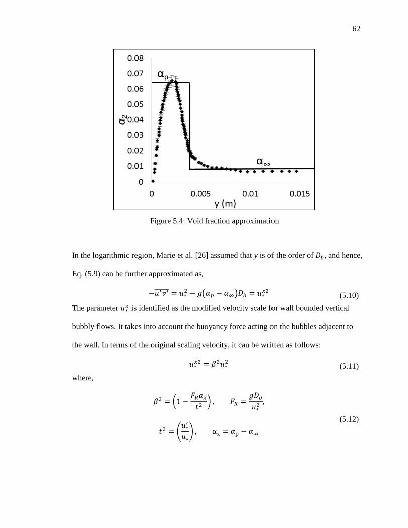
62
Figure 5.4: Void fraction approximation
In the logarithmic region, Marie et al. [26] assumed that y is of the order of 𝐷𝑏, and hence,
Eq. (5.9) can be further approximated as,
−𝑢′𝑣′ = 𝑢∗2 − 𝑔(𝛼𝑝 − 𝛼∞)𝐷𝑏 = 𝑢∗
𝑥2 (5.10)
The parameter 𝑢∗𝑥 is identified as the modified velocity scale for wall bounded vertical
bubbly flows. It takes into account the buoyancy force acting on the bubbles adjacent to
the wall. In terms of the original scaling velocity, it can be written as follows:
𝑢∗𝑥2 = 𝛽2𝑢∗
2 (5.11)
where,
𝛽2 = (1 −𝐹𝑅𝛼𝑥
𝑡2) , 𝐹𝑅 =
𝑔𝐷𝑏
𝑢∗2
,
𝑡2 = (𝑢∗
′
𝑢∗) , αx = αp − α∞
(5.12)
63
The non-dimensional parameter, 𝐹𝑅 is the frictional Froude number, which shows the
effect of gravity acting on the bubbles. By introducing the modified velocity scale in Eq.
(5.1), the logarithmic law of the wall can be rewritten as,
𝑢+𝑥 =1
𝜅𝑙𝑛𝑦+𝑥 + 𝐶𝑥 (5.13)
The variables,𝑢+𝑥 and 𝑦+𝑥 are non-dimensionalized using the modified velocity scale 𝑢∗𝑥.
It can be seen that the modified log-law has the same slope as Eq. (5.1), but the y
intercept, 𝐶𝑥 is no longer a constant, and is dependent on the parameter 𝛽 given by,
𝐶𝑥 − 𝐶 = 𝑠 (1
𝛽− 1) −
1
𝜅 (5.14)
The wall boundary conditions for 𝑘1 and 휀1 get modified as,
𝑘𝐵𝐶 =𝑢∗
√𝐶𝜇
; 휀𝐵𝐶 =𝑢∗
𝑥3
𝜅𝑦𝑤 (5.15)
5.4 Near-wall modeling
As discussed earlier, the void fraction distribution close to the wall has a characteristic
peak at a distance of bubble radius from the wall. This is a result of the shape of the
bubbles and the forces acting on it. In the near-wall region, the applicability of the
conventional two-fluid model is questionable. If the bubbles are assumed to be non-
deformable, the minimum distance a bubble center can be located from the wall is 𝑦 =
𝑅𝑏. For 𝑦 < 𝑅𝑏, the applicability of wall or lift force in the conventional form may be
questionable since, they represent the averaged forces that are supposed to act at the
bubble center.

64
Larrateguy et al. [27] and Moraga et al. [28] used a different approach to this problem.
The concept of bubble center averaging technique was adopted. It is summarized as
follows: the continuity and momentum equations for the liquid phase are solved in the
conventional manner. The dispersed phase conservation equations are obtained by
ensemble averaging the equations based on the bubble center indicator function η as
opposed to the phase indicator function 𝜒. The results obtained with the η averaged
equations, 𝛼2𝜂
and 𝑢2𝜂
are post-processed to obtain the primitive variables 𝛼2 and 𝑢2. This
is a purely geometric step where, the primitive variables are reconstructed based on the
shape of the bubbles. The proposed averaging technique thus separates the two aspects of
the bubble layer close to the wall, i.e., the bubble shape and the forces acting on the
bubbles.
However, this methodology is not applicable within the framework of the existing CFD
TFM codes since the equations need to be modified and the post-processing step needs to
be added. An alternate approach is proposed and validated in the current study. The
interfacial forces are removed up to a distance 𝑦𝑐 from the wall, which is calculated
based on the bubble geometry. In the present research, 𝑦𝑐 is calculated based on the
assumption that the bubbles are spherical and non-deformable. It must be noted that the
proposed technique can be applied to cases where the bubbles have other shapes such as
prolong or oblate spheroidal. Fig. 5.5 shows the comparison of the void fraction profile of
Marie et al. [26], with the assumed shape in the near-wall region used to calculate 𝑦𝑐. It
can be seen that there is a good agreement between the two. When the void fraction
profile is averaged, the void fraction distributions should have the same areas indicated
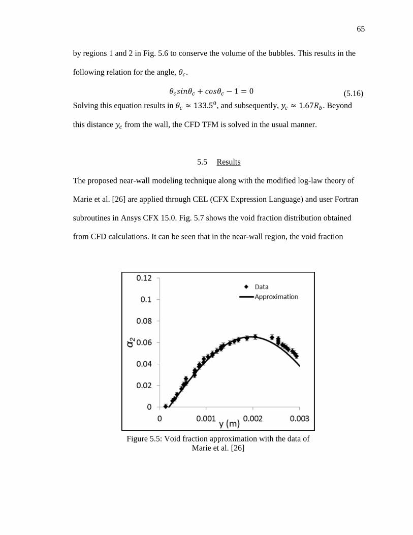
65
Figure 5.5: Void fraction approximation with the data of
Marie et al. [26]
by regions 1 and 2 in Fig. 5.6 to conserve the volume of the bubbles. This results in the
following relation for the angle, 𝜃𝑐.
𝜃𝑐𝑠𝑖𝑛𝜃𝑐 + 𝑐𝑜𝑠𝜃𝑐 − 1 = 0 (5.16)
Solving this equation results in 𝜃𝑐 ≈ 133.50, and subsequently, 𝑦𝑐 ≈ 1.67𝑅𝑏. Beyond
this distance 𝑦𝑐 from the wall, the CFD TFM is solved in the usual manner.
5.5 Results
The proposed near-wall modeling technique along with the modified log-law theory of
Marie et al. [26] are applied through CEL (CFX Expression Language) and user Fortran
subroutines in Ansys CFX 15.0. Fig. 5.7 shows the void fraction distribution obtained
from CFD calculations. It can be seen that in the near-wall region, the void fraction

66
Figure 5.6: Location of yc
profile gets averaged by using the proposed near-wall modeling approach. The free
stream value is in good agreement with the data of Marie et al. [26]. The results indicate
the presence of a double step function like distribution similar to the assumption of Marie
et al. [26] in developing the modified log-law. Hence, the proposed near-wall modeling
technique is consistent. The actual void fraction profile can later be reconstructed using
the geometry of the bubbles.
It can be seen in Fig. 5.8 that the slope of the liquid velocity profile is predicted well. The
effect of buoyancy force acting on the bubbles is reflected in the resulting velocity
distribution. In addition, it was possible to demonstrate convergence for both the void
fraction and the liquid velocity profiles which has not been done in the past. Once the
67
right near-wall modeling approach is used along with the wall functions based on the
modified log-law of Marie et al. [26], the void fraction and liquid velocity distributions
converge as seen in Fig. 5.9 and Fig. 5.10.
Finally, the applicability of the wall force model is addressed to a reasonable extent.
Typically, the wall force model of Antal et al. [37] is used to obtain the right shape of the
void fraction profile by varying the model coefficients according to the experimental
conditions. The model of Antal et al. [37] is developed based on the differential drainage
of the liquid around the bubble close to the wall, and calibrated with the experiments of
Nakoryakov, where the size of the bubbles is smaller (𝐷𝑏 = 0.87 𝑚𝑚) than the ones that
appear in air-water bubbly flows at atmospheric conditions. Also, the liquid flow
velocities used in the experiments of Nakoryakov are less (about 0.1 m/s) so that the
conditions were laminar. In practice, most of the dispersed bubbly flows are characterized
by shear induced and bubble induced turbulence (pseudo turbulence), and the bubble
motion becomes chaotic. In addition, when the bubbles come in contact with the walls
and the physical basis for the model of Antal et al. [37] may no longer be valid. The
proposed near-wall modeling approach eliminates the need for a wall force model.
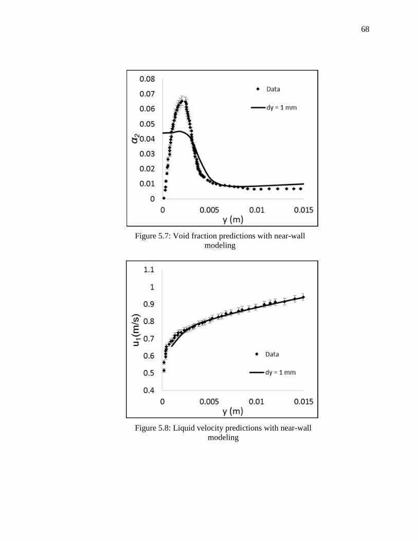
68
Figure 5.8: Liquid velocity predictions with near-wall
modeling
Figure 5.7: Void fraction predictions with near-wall
modeling

69
Figure 5.10: Liquid velocity convergence with near-wall
modeling
Figure 5.9: Void fraction convergence with near-wall
modeling

70
CHAPTER 6. CFD TFM SIMULATIONS
The Eulerian CFD TFM for transient calculations comprises of the set of equations given
by Eqs. (2.1), (2.2), which includes continuity and momentum equations for each of the
constituent phases along with the interphase interaction terms. The default CFD TFM
applied with LES modeling is observed to be ill-posed. The analysis presented in Chapter
3 is extended to 3-D CFD TFM calculations in this chapter. It is sought to achieve well-
posedness by adding essential short wavelength physics i.e., by introducing the interfacial
pressure difference and collision terms in to the TFM formulation. The proposed near-
wall modeling approach provides appropriate treatment of the void fraction distribution
in the near-wall region as described in Chapter 5. Well-posedness and consistency in
near-wall modeling are necessary to perform verification and validation with 3-D CFD
TFM.
6.1 Preliminary analysis
First, it is sought to demonstrate that well-posedness can be achieved by regularizing the
CFD TFM as done for 1-D TFM in Chapter 4. The travelling void wave problem similar
to the one seen in Chapter 4 is used as the test case. A 2D rectangular domain 0.1m by
1.0m is considered. All the four walls are treated as free-slip boundaries for both the
phases. The problem is hence made quasi 1-D, since the intention here is to focus on the

71
issues related to the well-posedness of the CFD TFM and isolating it from the other
aspects of CFD TFM viz., turbulence, and boundary conditions. To understand the
mathematical behavior of the TFM, it is important that a higher order numerical scheme
with a fine enough grid is used. This ensures that the contributions from numerical
viscosity are removed that may otherwise smoothen out the high frequency oscillations
arising from the ill-posed nature of the model, and make it appear well-posed.
Keeping this in mind, a uniform mesh with 1.25 mm grid spacing is used with a time step
size of 2 ms. The CFD calculations are performed using ANSYS Fluent 15.0 for a total
duration of 2 s. The initial condition is a Gaussian void fraction distribution
superimposed with a high frequency sine wave as shown in Fig. 6.1. The higher order
QUICK (Quadratic Upstream Interpolation for Convective Kinematics) scheme proposed
by Leonard [70] is used for spatial discretization. If the 1-D stencil shown in Fig. 4.1 is
considered, the numerical scheme is given by,
��1,𝑗 =𝜃
2(𝛼1,𝑐−1 + 𝛼1,𝑐) +
(1 − 𝜃)
2(3𝛼1,𝑐−1 − 𝛼1,𝑐−2) (6.1)
where, 𝜃 = 1/8 is commonly used. The bounded second order accurate implicit scheme
is used for temporal discretization [71] which is given by,
𝜕𝜙
𝜕𝑡=
𝜙𝑛+1 2⁄ − 𝜙𝑛−1 2⁄
Δ𝑡 (6.2)
where,
𝜙𝑛+1 2⁄ = 𝜙𝑛 +1
2𝛽𝑛+1 2⁄ (𝜙𝑛 − 𝜙𝑛−1) (6.3)
and,
𝜙𝑛−1 2⁄ = 𝜙𝑛−1 +1
2𝛽𝑛−1 2⁄ (𝜙𝑛−1 − 𝜙𝑛−2) (6.4)

72
Figure 6.1: Initial void fraction distribution
The bounding factors 𝛽𝑛+1 2⁄ , 𝛽𝑛−1 2⁄ are calculated internally based on the flow variables
[71]. Through the method of manufactured solutions, it is confirmed that the combination
of QUICK scheme along with the bounded second order implicit scheme in Ansys Fluent
15.0 has an order of accuracy higher than 1 as demonstrated in Appendix D.
When an ill-posed TFM formulation is used, it gives rise to pockets of high void fraction
concentrations as seen in Fig. 6.2 (a). After adding the appropriate short wavelength
physics (interfacial pressure, and collision force), the model is made well-posed. The
solution obtained (Fig. 6.2 (b)) is comparable to the solution in Fig. 4.5 for the 1 D TFM
having a shock at the rear and an expansion wave at the front.

73
Figure 6.2: Comparison of TFM results (a) ill-posed, (b) well-posed

74
6.2 Transient CFD TFM analysis
6.2.1 Experiment and problem set up
The work of Reddy Vanga [17] on two-phase bubbly plume is chosen to validate the
CFD TFM. A rectangular test section having a cross sectional area of 0.1 m by 0.02 m
was used to perform the experiments. The initial level of stagnant water in the test section
was varied between 0.2 m and 1.3 m. The gas superficial velocity ranged from 2 mm/s to
20 mm/s. The mean bubble diameter was observed to be 3 mm. Two distinct regions
were noted in the experiments. Close to the sparger, the bubbles rose in the stagnant
liquid column in the form of an oscillating plume, and this gives rise to an averaged
center-peaked void fraction profile as seen in Fig. 6.3. Far downstream, the bubbles rose
more uniformly resulting in a wall-peaked void fraction profile similar to the results in
the steady state calculations. In the region near the sparger, the dynamic behavior is
caused by the liquid recirculation zones on either side of the plume, and this will be the
focus to of the present study. The void fraction data obtained at 8 cm downstream from
the inlet will be used for benchmarking.
When CFD TFM is used with the LES approach, usually Milelli criterion [20] is followed,
according to which the grid size is restricted by ∆> 1.5𝐷𝑏. TFM being developed based
on continuum assumption, the restriction on the grid size based on the bubble diameter
makes no sense physically. Also, for the geometry of Reddy Vanga [17], if the Milelli
criterion [20] were to be followed, the minimum grid size that one could use is 5 mm, and
the depth of the channel in y direction is 20 mm resulting in 4 equally spaced nodes. It is
clear that a thorough convergence study can never be performed if the grid size restriction

75
based on the bubble diameter is to be imposed. Hence in the current study, the Milelli
criterion [20] is not used in selecting the grid size, but it is followed to determine the
filter size used in the sub-grid scale viscosity model of Smagorinsky [22]. In the current
calculations the sub-grid scale filter size is set to 5 mm.
The transient CFD calculations are performed with Ansys Fluent 15.0. The rectangular
domain used for the study is shown in Fig. 6.4. No slip wall BC is used for the liquid
phase, while free slip BC is used for the gas phase. Enhanced k-ε model is used to
prescribe the wall BC for the liquid phase velocity. The laminar and the logarithmic law
of the wall are blended using the function proposed by Kader [72] resulting in,
𝑢+ = 𝑒Γ𝑢𝑙𝑎𝑚+ + 𝑒
1Γ⁄ 𝑢𝑡𝑢𝑟𝑏
+ (6.5)
where,
Γ =𝑎(𝑦+)4
1 + 𝑏𝑦+ (6.6)
where, a = 0.01, b = 5. It is concluded in Fluent theory manual [71] that the blending
function approach predicts the right asymptotic behavior for large and small y+, and at the
same time it gives a reasonable prediction for y+ in the range 3 < y+ < 10. This is suitable
in the current study since the Reynolds number associated with the flow in general is very
less.
The grid convergence test is performed with three different grid sizes, 5 mm, 2.5 mm and
1.25 mm. The time step sizes chosen are 8 ms, 4 ms, and 2 ms respectively. QUICK
scheme is chosen for the spatial discretization and bounded second order implicit scheme

76
for the temporal discretization. Time averaged void fraction profiles are obtained using
monitor lines at 8 cm from the inlet.
6.2.2 Results
Initially, the basic CFD TFM with the proposed near-wall modeling is used to simulate
the plume oscillations, i.e, without the interfacial pressure or collision mechanism. The
coarse mesh with Δx = 5 mm gives a well-behaved numerical solution as seen in Fig. 6.5.
The plume structure at three different time frames are shown, and it can be noticed that
the CFD TFM is capable of capturing the dynamics of the instability. When the mesh is
refined, the solution starts to show high void fraction regions in the domain as seen in Fig.
6.6 (b). This is similar to the observations made in the case of traveling void wave
problem (Fig. 6.2 (a)), and it again indicates the ill-posedness in the basic CFD TFM. The
non-physical high concentration regions are not seen when the coarse mesh is used
because of the inherent numerical diffusion that arises from the coarse discretization.
When the properly posed CFD TFM is used by including the contributions from
interfacial pressure and collision terms, the solution obtained with the refined mesh is
free from numerical instabilities as seen in Fig. 6.7 (b).

77
Figure 6.3: Structure of the plume
of Reddy Vanga [17]

78
Figure 6.4: Computational domain

79
Figure 6.5: Instantaneous contours of α2, Δx = 5 mm

80
Figure 6.6: Contours of α2 with ill-posed TFM (a) Δx = 5 mm,
(b) Δx = 1.25 mm

81
Figure 6.7: Contours of α2 with well-posed TFM (a) Δx = 5
mm, (b) Δx = 1.25 mm

82
Well-posedness is an important feature of the numerical TFM without which,
convergence studies will no longer be feasible. At the same time, regularization needs to
be done by adding physically motivated terms in order to avoid over damping of the
system. Now that the CFD TFM is made well-posed by adding appropriate short
wavelength physics, the grid convergence test is performed. Time series of the void
fraction and liquid velocities are obtained at the monitor point located at the coordinates
(0.05, 0.01, 0.2), where it is expected to be characterized by liquid eddies having a wide
range of frequencies. For the case of 5 mm mesh, the time series shows a periodic
behavior characterized by specific frequencies as shown in Fig. 6.8. Typically, phase
space plots are used to describe the non-linear dynamics to characterize the system. The
given time series and its lagged series are used to visualize the trajectories in the phase
space, using a suitable time lag (0.5 s in the current study). As seen in Fig. 6.9, the phase
space plot indicates a closed trajectory that is followed periodically. The time series and
the phase space plots clearly indicate limit cycle behavior. The other parameter
commonly used for statistical analysis is the Fast Fourier Transform (FFT) spectra. The
time series is transformed in to Fourier frequency domain by performing an FFT, where
the time-velocity or time-void fraction data sets are converted to frequency-amplitude
data sets. The amplitude in the frequency domain is defined by,
|𝐴(𝜑)| =
𝐹𝐹𝑇(𝜑′)
𝑁2⁄
(6.7)
where, 𝜑′ represents the series of fluctuations in 𝜑 given by,
𝜑′ = 𝜑 − �� (6.8)

83
where, �� represents the mean 𝜑 calculated from the time series. In the present study, 𝜑 =
[𝛼2, 𝑢1] is used for spectral analysis. The FFT spectra of both 𝛼2, and 𝑢1 (Fig. 6.10, Fig.
6.11) exhibit distinct isolated frequencies. This indicates a lack of interaction between the
different Fourier components that exists for a turbulent flow characterized by chaos.
When a 2.5 mm mesh is used, the time series of liquid velocity is shown in Fig. 6.12,
which can be noticed to be non-periodic. On the phase space plot (Fig. 6.13), the
trajectories are inter-woven and are not distinct as opposed to well-defined trajectories
that is seen with the 5 mm mesh simulations (Fig. 6.9). This is a clear indicator of a
chaotic behavior. The FFT spectra (Fig. 6.14, Fig. 6.15) indicate continuous distributions
on the frequency domain. This makes it possible to cascade or transfer energy through the
interacting Fourier modes. A similar set of results is obtained for the case of 1.25 mm
mesh, which exhibits chaotic behavior as well (Fig. 6.16 – Fig. 6.19).
It can be seen (Fig. 6.20, Fig. 6.21) that the void fraction and liquid velocity results
obtained with the 2.5 mm and 1.25 mm mesh show good spectral convergence. Another
significant feature is the prevalence of -5/3 slope in the turbulent kinetic energy (TKE)
spectra for both 𝑗𝑔 = 2 𝑚𝑚/𝑠, and 𝑗𝑔 = 6 𝑚𝑚/𝑠 cases as seen in Fig. 6.22, Fig. 6.23.
Finally, the results using the CFD TFM developed in the present study is compared with
the void fraction data of Reddy Vanga [17] as shown in Fig. 6.24, which indicates a good
convergence as well. Thus, it is shown here that the 3-D CFD TFM for wall-bounded
bubbly flows can be made well-posed and convergent by adding appropriate short
wavelength physics along with a consistent near-wall modeling.
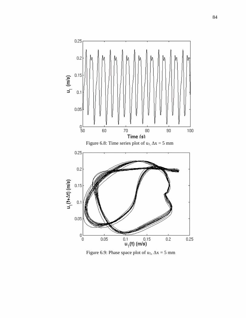
84
Figure 6.8: Time series plot of u1, Δx = 5 mm
Figure 6.9: Phase space plot of u1, Δx = 5 mm

85
Figure 6.10: FFT speactra of α2, Δx = 5 mm
Figure 6.11: FFT spectra of u1, Δx = 5 mm

86
Figure 6.12: Time series plot of u1, Δx = 2.5 mm
Figure 6.13: Phase space plot of u1, Δx = 2.5 mm
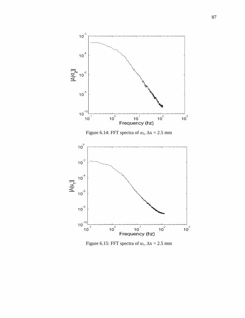
87
Figure 6.14: FFT spectra of α2, Δx = 2.5 mm
Figure 6.15: FFT spectra of u1, Δx = 2.5 mm

88
Figure 6.16: Time series plot of u1, Δx = 1.25 mm
Figure 6.17: Phase space plot of u1, Δx = 1.25 mm

89
Figure 6.18: FFT spectra of α2, Δx = 1.25 mm
Figure 6.19: FFT spectra of u1, Δx = 1.25 mm

90
Figure 6.20: Convergence of α2 spectra
Figure 6.21: Convergence of u1 spectra
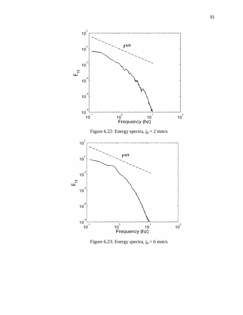
91
Figure 6.22: Energy spectra, jg = 2 mm/s
Figure 6.23: Energy spectra, jg = 6 mm/s

92
Figure 6.24: Comparison of α2 distribution with data, jg = 2 mm/s

93
CHAPTER 7. CONCLUSIONS AND RECOMMENDATIONS
7.1 Summary of Work
In Chapter 2, the 3-D TFM of Ishii [2] for incompressible vertical bubbly two-phase
flows along with the closure relations for the interfacial momentum transfer terms and
turbulence modeling were described. The simplified 3-D TFM was the starting point to
derive the area-averaged 1-D TFM, which is efficient for analysis where significant
changes occur in the direction of the flow. Only the momentum transfer contributions
from drag, and virtual mass forces were preserved since they are dominant in the axial
direction. If the assumptions are made that volumetric flux is constant, and the density
ratio 𝜌2 𝜌1⁄ ≪ 1, this 4-equation TFM can be reduced to a fixed-flux 2-equation TFM,
which is an appropriate simplification in the context of short wavelength physics. It may
be suitable for air-water two-phase flows as the density ratio is much lesser than 1.
However, it is inappropriate to analyze system or integral instabilities, where the constant
flux assumption breaks down.
In Chapter 3, the complete linear stability analysis of the 1-D TFM was presented. The
nature of the eigenvalues determine the mathematical behavior of the model. For the
TFM to be well-posed, it needs to be hyperbolic which is determined by the material
roots being real. Previous results obtained by Pauchon and Banerjee [1], Haley et al. [7],
94
and Park et al. [8] were confirmed. To overcome the issue of conditional well-posedness,
the mechanism of collision is considered. The model of Alajbegovic et al. [15] is adapted
to develop a correlation suitable for bubbly two-phase flows. It was shown that by adding
collision mechanism, the TFM can be made unconditionally well-posed. Additionally, the
developed collision force model is suitable in any of the modeling frameworks, unlike the
original model which depends on the particle stress tensor that is calculated only when
Reynolds stress transport modeling is performed. It was also shown that the model is
capable of predicting the correct right kinematic wave velocities. Dispersion analysis was
used to demonstrate the need for physical regularization. It was shown that viscous
stresses alone are not sufficient to stabilize the TFM.
In Chapter 4, numerical simulations were performed with void propagation and 1-D
fixed-flux 2-equation TFM to understand the non-linear evolution of the kinematic void
wave. A traveling void wave problem was used to demonstrate the issue of ill-posedness.
It was shown that when an incomplete TFM formulation is used, it results in high
frequency oscillations. When the physical mechanisms of interfacial pressure and bubble
collisions were added, the TFM becomes properly posed as an initial value problem. This
eliminated the non-physical high frequency oscillations. Also, it was shown that when the
flow is stable, the results obtained with the drift flux void propagation equation and
fixed-flux 2-equation TFM are identical. The wave propagation velocity is determined by
the drift velocity correlation for the void propagation equation and by the drag coefficient
for the fixed-flux TFM.
95
In Chapter 5, it was shown that the results from 1-D linear and non-linear analysis can be
extended to 3-D CFD TFM calculations. It was demonstrated with the traveling wave
problem that the CFD TFM can be well-posed with the inclusion of missing short
wavelength physics, i.e. interfacial pressure and collision forces. The issue of the near-
wall modeling was addressed with a new approach that converges, and is consistent with
the modified logarithmic law of the wall theory of Marie et al. [26]. Furthermore, the
near-wall modeling approach used in the present study eliminated the need for a wall
force model. The experiment of Reddy Vanga [17] was used to validate the well-posed 3-
D CFD TFM developed in the present study. It was observed that the CFD calculation
with the coarse mesh resulted in a limit cycle while for the case of a turbulent bubbly
two-phase flow, one may expect chaos. However, when the refined meshes were used,
the solutions were chaotic. Thus, it was shown that the use of grid size restrictions (eg.
Milelli, [20]) may lead to inappropriate physical results. Since the TFM of Ishii [2] or
Vernier and Delhaye [3] was developed based on continuum approach, it should be free
from such criteria. In addition, it was also observed that the CFD calculations on bubble
column revealed the -5/3 Komogorov scaling typically used to characterize the eddies in
the inertial range for turbulent flows. The well-posed Eulerian CFD TFM is shown to be
convergent in a statistical sense by comparing the FFT spectra and time averaged void
fraction profiles.
In Appendix A and Appendix B, the exact analytical solutions to the eigenvalues were
presented after including interfacial pressure and collision force terms in the TFM
formulation. In Appendix C, the effect of compressibility on the eigenvalues of the TFM
96
was discussed. It was shown that the acoustic roots do not affect the well-posedness of
the TFM. Finally in Appendix D, the method of manufactured solutions is presented in
the framework of 1-D TFM code and CFD TFM of ANSYS Fluent 15.0. It was verified
that the numerical schemes used in the present study had orders of accuracy higher than
one.
It is hence shown that the TFM may become well-posed as an initial value problem if the
appropriate physics are added. For the case of bubbly flows, the mechanism of collision
is deemed necessary to regularize the TFM and make it unconditionally well-posed. This
aspect of the numerical TFMs (1-D or 3-D CFD) is important to make convergence study
feasible. Otherwise, the solution gets affected by high frequency oscillations when the
mesh is refined as demonstrated. In addition, for the case of 3-D TFM, the near-wall
region needs to be treated appropriately in order to make the solution consistent with the
boundary conditions and to obtain convergence in this region.
7.2 Recommendations
The author would like to make the following recommendations based on the current TFM
analysis:
1. The convergent well-posed TFM developed in the present study is capable of
being applied to flows where local void fractions are higher than 26 %. Hence, a
possible extension of the current work may be to explore the flow regime
transition, and to understand the phenomena from the perspective of void wave

97
instability. It would be interesting to observe if this instability could be modeled
for vertical two-phase flows that may eventually lead to flow regime transition.
2. The current research can be extended to understand the dynamic behavior of two-
phase jets. The proposed TFM can be used with an appropriate three field two-
fluid model similar to Lopez de Bertodano et al. [73], and Prabhudharwadkar et al.
[74]. Experiments of Sun et al. [75] on a rectangular channel give measurements
of void fraction distribution data of the small and big bubbles that can be used to
validate the model.
3. In addition, the applicability of the well-posed TFM in conjunction with the
interfacial area transport equation (IATE) can be explored for 1-group and 2-
group cases. The resulting model will be more predictive, since the morphology
of the bubbles will be determined by the interfacial area concentration, which is
obtained by solving the transport equation.

98
APPENDICES
Figure C.7.1:
Comparison of
acoustic speeds
with Henry et al.
(1971)

98
Appendix A Characteristics
One of the methods to determine the well-posedness of a mathematical model is to
analyse the eigenvalues or characteristics of a system of equation. It is demonstrated by
Ramshaw and Trapp [4] that in the limit of 𝜆 → 0 the dispersion analysis and the
characteristics analysis become identical. For the case of 4 equation 1-D TFM, the
governing equations can be recast into
𝐴𝜕
𝜕𝑡𝜙 + 𝐵
𝜕
𝜕𝑥𝜙 + 𝐷
𝜕2
𝜕𝑥2𝜙 + 𝐹 = 0 (A.1)
The coefficient matrix A is given by,
𝐴 = [
𝐴11 0 0 0𝐴21 0 0 0
0 𝐴32 𝐴33 00 𝐴42 𝐴43 0
] (A.2)
where,
𝐴11 = 1
𝐴21 = 1
𝐴32 = 𝜌1(1 − 𝛼2) + 𝐶𝑉𝑀𝜌1𝛼2
𝐴33 = −𝐶𝑉𝑀𝜌1𝑢2𝛼2
𝐴42 = −𝐶𝑉𝑀𝜌1𝛼2
𝐴43 = 𝜌2
𝛼2 + 𝐶𝑉𝑀𝜌1
𝛼2
(A.3)
The coefficient matrix B is given by,
𝐵 = [
𝐵11 𝐵12 0 0𝐵21 0 𝐵23 0𝐵31 𝐵32 𝐵33 𝐵34
0 𝐵42 𝐵43 𝐵44
] (A.4)

99
where,
𝐵11 = 𝑢1
𝐵12 = −(1 − 𝛼2)
𝐵21 = 𝑢2
𝐵23 = 𝛼2
𝐵31 = −𝐶𝑃𝜌1𝑢𝑟2
𝐵32 = 𝑢1(𝜌1(1 − 𝛼2) + 𝐶𝑉𝑀𝜌1𝛼2)
𝐵33 = −𝐶𝑉𝑀𝜌1𝑢2𝛼2
𝐵34 = 1 − 𝛼2
𝐵42 = −𝐶𝑉𝑀𝜌1𝑢2𝛼2 + 2𝐶𝑃𝜌1𝑢𝑟𝛼2
𝐵43 = −2𝐶𝑃𝜌1𝑢𝑟𝛼2 + 𝑢2(𝜌2𝛼2 + 𝐶𝑉𝑀𝜌1𝛼2)
𝐵44 = 𝛼2
(A.5)
The coefficient matrix D is given by,
𝐷 = [
0 0 0 00 0 0 00 𝐷32 0 00 0 𝐷43 0
] (A.6)
where,
𝐷32 = 𝜌1(𝜈1 + 𝜈1,𝑆𝑎𝑡𝑜)
𝐷43 = 𝜌2𝜈2 (A.7)
The source term matrix F is given by,
𝐹 = [
00
−𝜌1(1 − 𝛼2)𝑔 − 𝑀2𝑖𝐷
𝜌2𝛼2𝑔 + 𝑀2𝑖𝐷
] (A.8)

100
The constraint equation for the eigenvalues is given by,
Det(𝐴𝜆 − 𝐵) = 0 (A.9)
The resulting eigenvalues corresponding to the material waves are,
𝜆1,2 = 𝜉 ± √𝜂 (A.10)
where,
𝜉 =𝜌1𝐶𝑉𝑀(𝛼2𝑢1 + 𝛼1𝑢2) − 𝛼1(𝜌1𝐶𝑃𝑢𝑟 − 𝜌1𝛼2𝑢1 − 𝜌2𝛼1𝑢2)
𝜌1𝐶𝑉𝑀 + 𝛼1(𝜌1𝛼2 + 𝜌2𝛼1) (A.11)
𝜂 = 𝜂1 + 𝜂2𝜂3 (A.12)
where,
𝜂1 = 𝜉2 (A.13)
𝜂2 =1
𝛼2(𝜌1𝐶𝑉𝑀 + 𝛼1(𝜌1𝛼2 + 𝜌2𝛼1)) (A.14)
𝜂3 = −𝛼2 (𝜌1𝐶𝑉𝑀(𝛼2𝑢12 + 𝛼1𝑢2
2)
+ 𝛼1(𝜌1𝛼2𝑢12 + 𝜌2𝛼1𝑢2
2
− 𝐶𝑃𝜌1𝑢𝑟(2(𝛼2𝑢1 + 𝛼1𝑢2) + 𝛼2𝑢𝑟)))
(A.15)
101
Appendix B Collision
The model proposed by Alajbegovic et al. [15] is used in the current study. It is given by,
𝑀𝑐𝑜𝑙𝑙 = −∇. [(𝜌2 + 𝜌1𝐶𝑉𝑀)𝑔(𝛼2)𝛼22(2𝑢2
′ 𝑢2′ + 𝑢2
′ . 𝑢2′ 𝐼)] (B.1)
where, I represents the identity tensor. Assuming the bubbles to be in turbulence
equilibrium with the liquid, the stress tensors in the two medium can be related by,
𝑢2′ 𝑢2
′ =1
1 +𝜏𝑝
𝜏𝑐⁄
𝑢1′ 𝑢1
′ (B.2)
where, 𝜏𝑐 represents the time constant for the bubble induced eddies given by,
𝜏𝑐 =𝐷𝑏
𝑢𝑟 (B.3)
and 𝜏𝑝 represents the particle relaxation time which can be obtained from the force
balance on a single bubble given by,
(𝜌2 + 𝜌1𝐶𝑉𝑀)𝑑𝑢2
𝑑𝑡= −
3
4
𝐶𝐷𝑅𝑒𝜇1𝑢2
𝐷𝑏2 (B.4)
where,
𝜏𝑝 =4
3
(𝜌2 + 𝜌1𝐶𝑉𝑀)𝐷𝑏2
𝐶𝐷𝑅𝑒𝜇1 (B.5)
For the case of Stokes’ flow, 𝜏𝑝
𝜏𝑐⁄ ≪ 1 , whereas for the case of air-water turbulent
bubbly flows, the ratio 𝜏𝑝
𝜏𝑐⁄ may be much higher. Further, the bubble induced
component of the stress tensor in the continuous phase is given by Bertodano et al. [41]
as,
𝑢1′ 𝑢1
′ = [
4/5 0 00 3/5 00 0 3/5
]1
2𝐶𝑉𝑀𝛼2|𝑢𝑟|2 (B.6)

102
If an assumption is made that, the stress tensor associated with the bubbles is isotropic,
and using Eq. (B.2) - (B.6), Eq. (B.1) can be simplified as,
𝑀𝑐𝑜𝑙𝑙 = −𝐶𝑐𝑜𝑙𝑙𝜌1𝐶𝑉𝑀2 ∇. [𝑔(𝛼2)𝛼2
3|𝑢𝑟|2𝐼] (B.7)
For the case of linear stability analysis, the momentum transfer term due to collisions in
1-D can be reduced to,
𝑀𝑐𝑜𝑙𝑙 = −𝐶𝑐𝑜𝑙𝑙𝜌1𝐶𝑉𝑀2 ((3𝛼2
2𝑢𝑟2𝑔(𝛼2) + 𝛼2
3𝑢𝑟2
𝑑𝑔(𝛼2)
𝑑𝛼2)
𝜕𝛼2
𝜕𝑥
+ 2𝛼23𝑢𝑟𝑔(𝛼2)
𝜕𝑢𝑟
𝜕𝑥)
(B.8)
The pair correlation function of Carnahan and Starling [11] is used, given by,
𝑔(𝛼2) =2 − 𝛼2
2(1 − 𝛼2)3 (B.9)
It must be kept in mind that the collision force model used here is based on hard sphere
collisions which may not be sufficient to represent the bubble-bubble interactions seen in
reality.
When the collision term is added to the TFM, the elements 𝐵41, 𝐵43, and 𝐵43 become,
𝐵41 = 𝐶𝑐𝑜𝑙𝑙𝜌1𝐶𝑉𝑀2 (3𝛼2
2𝑢𝑟2𝑔(𝛼2) + 𝛼2
3𝑢𝑟2
𝑑𝑔(𝛼2)
𝑑𝛼2) (B.10)
𝐵42 = −2𝐶𝑐𝑜𝑙𝑙𝜌1𝐶𝑉𝑀2 𝛼2
3𝑢𝑟𝑔(𝛼2) − 𝐶𝑉𝑀𝜌1𝑢2𝛼2 + 2𝐶𝑃𝜌1𝑢𝑟𝛼2 (B.11)
𝐵43 = 2𝐶𝑐𝑜𝑙𝑙𝜌1𝐶𝑉𝑀2 𝛼2
3𝑢𝑟𝑔(𝛼2) − 2𝐶𝑃𝜌1𝑢𝑟𝛼2 + 𝑢2(𝜌2𝛼2 + 𝐶𝑉𝑀𝜌1𝛼2) (B.12)
The eigenvalues corresponding to the material waves get modified as,
𝜆′1,2 = 𝜉′ ± √𝜂′ (B.13)
where,
103
𝜉′ =𝐶𝑈𝛼1 − 2𝛼2(𝜌1𝐶𝑉𝑀(𝛼2𝑢1 + 𝛼1𝑢2) − 𝛼1(𝜌1𝐶𝑃𝑢𝑟 − 𝜌1𝛼2𝑢1 − 𝜌2𝛼1𝑢2))
−2𝛼2(𝜌1𝐶𝑉𝑀 + 𝛼1(𝜌1𝛼2 + 𝜌2𝛼1)) (B.14)
𝜂′ = 𝜂′1 + 𝜂′2(𝜂′3 + 𝜂′4) (B.15)
where,
𝜂′1 = 𝜉′2 (B.16)
𝜂′2 =1
𝛼2(𝜌1𝐶𝑉𝑀 + 𝛼1(𝜌1𝛼2 + 𝜌2𝛼1)) (B.17)
𝜂′3 = 𝐶𝑈𝛼1(𝛼2𝑢1 + 𝛼1𝑢2) (B.18)
𝜂′4 = −𝛼2 (𝐵41𝛼12 + 𝜌1𝐶𝑉𝑀(𝛼2𝑢1
2 + 𝛼1𝑢22)
+ 𝛼1(𝜌1𝛼2𝑢12 + 𝜌2𝛼1𝑢2
2
− 𝐶𝑃𝜌1𝑢𝑟(2(𝛼2𝑢1 + 𝛼1𝑢2) + 𝛼2𝑢𝑟)))
(B.19)
where,
𝐶𝑈 = 2𝐶𝑐𝑜𝑙𝑙𝜌1𝐶𝑉𝑀2 𝛼2
3𝑢𝑟𝑔(𝛼2) (B.20)
Finally, the collision term can also be cast into 2-equation TFM framework. The
coefficient of the void fraction gradient term appearing in Eq. (2.51) gets modified as,
𝐵21′ = 𝐵21 −
𝐶𝑐𝑜𝑙𝑙𝐶𝑉𝑀2
(1 − 𝛼1)(
𝛼1(1 − 𝛼1)
𝐶𝑉𝑀 + 𝛼1(1 − 𝛼1)) (𝐶1 + 𝐶2 + 𝐶3) (B.21)
where, 𝐵21 is given by Eq. (2.52). The terms 𝐶1, 𝐶2, and 𝐶3 are given by,
𝐶1 = −3(1 − 𝛼1)2𝑢𝑟2𝑔(𝛼2) (B.22)

104
𝐶2 = 2𝑢𝑟(1 − 𝛼1)𝑔(𝛼2) (B.23)
𝐶3 = (1 − 𝛼1)3𝑢𝑟2
𝑑𝑔(𝛼2)
𝑑𝛼2 (B.24)
The coefficient of the velocity gradient term appearing in Eq. (2.51) gets modified as,
𝐵22′ = 𝐵22 −
𝐶𝑐𝑜𝑙𝑙𝐶𝑉𝑀2
(1 − 𝛼1)(
𝛼1(1 − 𝛼1)
𝐶𝑉𝑀 + 𝛼1(1 − 𝛼1)) 𝐶4 (B.25)
𝐶4 = −2𝑢𝑟(1 − 𝛼1)2𝑔(𝛼2) (B.26)

105
Appendix C Effect of compressibility
Some of the commonly observed two-phase flows occur at conditions where
compressibility of the phases may need to be considered. The ideal gas law is used to
relate density in terms of pressure. Including the effect of compressibility in the 1-D TFM
formulation, the governing equations can be written as,
𝜕𝛼1
𝜕𝑡+
𝜕
𝜕𝑥𝛼1𝑢1 +
𝛼1
𝜌1𝑐12 (
𝜕𝑝
𝜕𝑡+ 𝑢1
𝜕𝑝
𝜕𝑥) = 0 (C.1)
𝜕𝛼2
𝜕𝑡+
𝜕
𝜕𝑥𝛼2𝑢2 +
𝛼2
𝜌2𝑐22 (
𝜕𝑝
𝜕𝑡+ 𝑢2
𝜕𝑝
𝜕𝑥) = 0 (C.2)
𝜌1𝛼1 (𝜕𝑢1
𝜕𝑡+ 𝑢1
𝜕𝑢1
𝜕𝑥)
= −𝛼1
𝜕𝑝1
𝜕𝑥+
𝜕
𝜕𝑥𝛼1(𝜏𝑘𝑧𝑧 + 𝜏𝑘𝑧𝑧
𝑇 ) − 𝛼1𝜌1𝑔𝑥 − 𝑀2𝑖𝑉𝑀 − 𝑀2𝑖
𝐷
− (𝑝𝑘𝑖 − 𝑝𝑘)𝜕𝛼1
𝜕𝑥
(C.3)
𝜌2𝛼2 (𝜕𝑢2
𝜕𝑡+ 𝑢2
𝜕𝑢2
𝜕𝑥) +
𝑢1
𝑐12
𝜕𝑝
𝜕𝑥= −𝛼2
𝜕𝑝1𝑖
𝜕𝑥− 𝛼2𝜌2𝑔𝑥 + 𝑀2𝑖
𝑉𝑀 + 𝑀2𝑖𝐷 (C.4)
With regards to the system of equations seen in Appendix A, the following modifications
need to be done
𝐴14 =𝛼1
𝜌1𝑐12
𝐴24 =𝛼2
𝜌2𝑐22
(C.5)
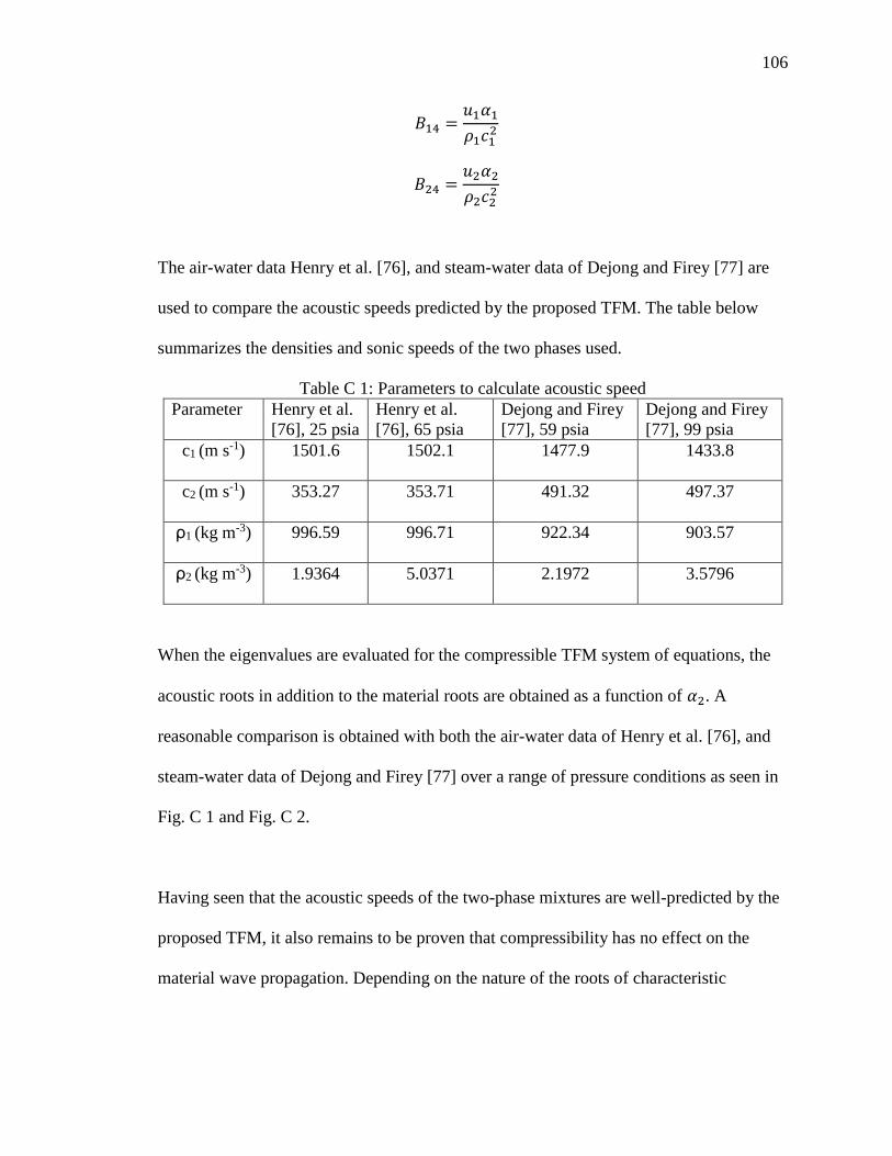
106
𝐵14 =𝑢1𝛼1
𝜌1𝑐12
𝐵24 =𝑢2𝛼2
𝜌2𝑐22
The air-water data Henry et al. [76], and steam-water data of Dejong and Firey [77] are
used to compare the acoustic speeds predicted by the proposed TFM. The table below
summarizes the densities and sonic speeds of the two phases used.
Table C 1: Parameters to calculate acoustic speed
Parameter Henry et al.
[76], 25 psia
Henry et al.
[76], 65 psia
Dejong and Firey
[77], 59 psia
Dejong and Firey
[77], 99 psia
c1 (m s-1) 1501.6 1502.1 1477.9 1433.8
c2 (m s-1) 353.27 353.71 491.32 497.37
ρ1 (kg m-3) 996.59 996.71 922.34 903.57
ρ2 (kg m-3) 1.9364 5.0371 2.1972 3.5796
When the eigenvalues are evaluated for the compressible TFM system of equations, the
acoustic roots in addition to the material roots are obtained as a function of 𝛼2. A
reasonable comparison is obtained with both the air-water data of Henry et al. [76], and
steam-water data of Dejong and Firey [77] over a range of pressure conditions as seen in
Fig. C 1 and Fig. C 2.
Having seen that the acoustic speeds of the two-phase mixtures are well-predicted by the
proposed TFM, it also remains to be proven that compressibility has no effect on the
material wave propagation. Depending on the nature of the roots of characteristic

107
polynomial, the system is classified as either well-posed or ill-posed. First, the effect of
adding interfacial pressure and virtual mass is shown by comparing the plots of
characteristic polynomial for different values of 𝛼2 (Fig. C.3). It can be seen that the
results are in accordance with Fig. 3.1, where, the well-posedness of the TFM is restricted
to α2 < 0.26. Fig. C 3 shows that for α2 = 0.2, 0.24, a total of 4 real roots are obtained, of
which 2 pertain to the material wave, and hence the system is classified as well-posed
under those conditions. However, for the case of α2 = 0.28, only two real roots are
obtained pertaining to the acoustic speeds since the TFM becomes ill-posed.
Fig. C 4 shows the effect of adding collision mechanism for the case of α2 = 0.28., where
the TFM was ill-posed previously. It is seen that there exist 4 real roots, 2 corresponding
to the acoustic wave speeds of the mixture and 2 corresponding to the material wave
speeds, since the TFM becomes well-posed by adding the inter-bubble collision term.
This is in accordance with Fig. 3.3 where it is shown that the TFM becomes
unconditionally well-posed.
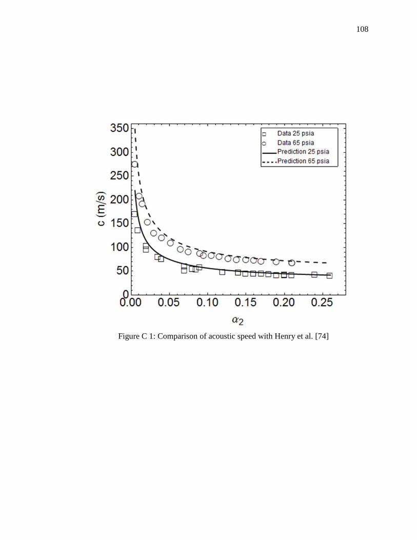
108
Figure C 1: Comparison of acoustic speed with Henry et al. [74]

109
Figure C 2: Comparison of acoustic speeds with Dejong and Firey [75]

110
Figure C 3: Dispersion relation without collision for different α2

111
Figure C 4: Dispersion relation with collision, α2 = 0.28

112
Appendix D Method of Manufactured Solutions
Code verification is a necessary procedure to be done to assess the order of accuracy. The
usual procedure is to perform numerical calculations with the numerical code for a case
where the exact solution is known. The numerical solution obtained is then compared
with the exact solution using one of the standard norms for different grid sizes to
compute the order of accuracy. However, for the case of TFM, there is no known solution
that makes use of all the terms appearing in the TFM.
The alternative is to adopt the method of manufactured solutions proposed by Roache
[78]. The procedure is straightforward to be implemented in any numerical code. A form
of an exact solution is picked, which is then substituted into the governing equations
resulting in additional source terms. These terms are then added to the original source
terms present in the model on the right hand side of the respective equations. When the
system of equations is solved, the difference between the numerical solution and the
exact proposed solution is used to obtain the order of convergence
The 1-D 2- equation TFM given by Eqs. (2.50), (2.51) can be formulated as,
𝑆𝛼1=
𝜕𝛼1
𝜕𝑡+ 𝑢1
𝜕𝛼1
𝜕𝑥+ 𝛼1
𝜕𝑢1
𝜕𝑥 (D.1)
𝑆𝑢1=
𝜕𝑢1
𝜕𝑡+ 𝐵21
𝜕𝛼1
𝜕𝑥+ 𝐵22
𝜕𝑢1
𝜕𝑥− 𝑆 (D.2)
The following form of exact solution is used,

113
��1 = 𝐶1 + 𝐷1𝑠𝑖𝑛(𝜅(𝑥 − 𝑐𝑡)) (D.3)
��1 = 𝐶2 + 𝐷2𝑠𝑖𝑛(𝜅(𝑥 − 𝑐𝑡)) (D.4)
Substituting Eq. (D.3) and Eq. (D.4) in Eqs. (D.1), (D.2), the following source terms can
be obtained
𝑆𝛼1= 𝜅 (−𝑐𝐷1𝑐𝑜𝑠(𝜅(𝑥 − 𝑐𝑡)) + 𝐶1𝐷2𝑐𝑜𝑠(𝜅(𝑥 − 𝑐𝑡))
+ 𝐶2𝐷1𝑐𝑜𝑠(𝜅(𝑥 − 𝑐𝑡))
+ 2𝐷1𝐷1𝑠𝑖𝑛(𝜅(𝑥 − 𝑐𝑡))𝑐𝑜𝑠(𝜅(𝑥 − 𝑐𝑡)))
(D.5)
𝑆𝑢1= 𝜅 (−𝑐𝐷2𝑐𝑜𝑠(𝜅(𝑥 − 𝑐𝑡)) + ��21𝐷1𝑐𝑜𝑠(𝜅(𝑥 − 𝑐𝑡))
+ ��22𝐷2𝑐𝑜𝑠(𝜅(𝑥 − 𝑐𝑡))) − �� (D.6)
where, ��21, ��21 are the coefficients 𝐵21, 𝐵22as functions of the exact solution ��1, ��1. ��
represents the RHS of Eq. (2.51) using ��1, ��1. When the proposed form of the exact
solution is used, the governing equations get modified as,
𝜕𝛼1
𝜕𝑡+ 𝑢1
𝜕𝛼1
𝜕𝑥+ 𝛼1
𝜕𝑢1
𝜕𝑥= 𝑆𝛼1
(D.7)
𝜕𝑢1
𝜕𝑡+ 𝐵21
𝜕𝛼1
𝜕𝑥+ 𝐵22
𝜕𝑢1
𝜕𝑥= 𝑆 + 𝑆𝑢1
(D.8)
The values of the constants are summarized in Table D 1. The domain considered for the
problem extends from – 𝜋 to – 𝜋. The number of grid points considered for the problem
are N = 160, 320, 640, 1280. The calculations are performed for a total duration of 4 s by
fixing the time step based on ∆𝑡∆𝑥⁄ = 0.05. The resulting solutions are compared with
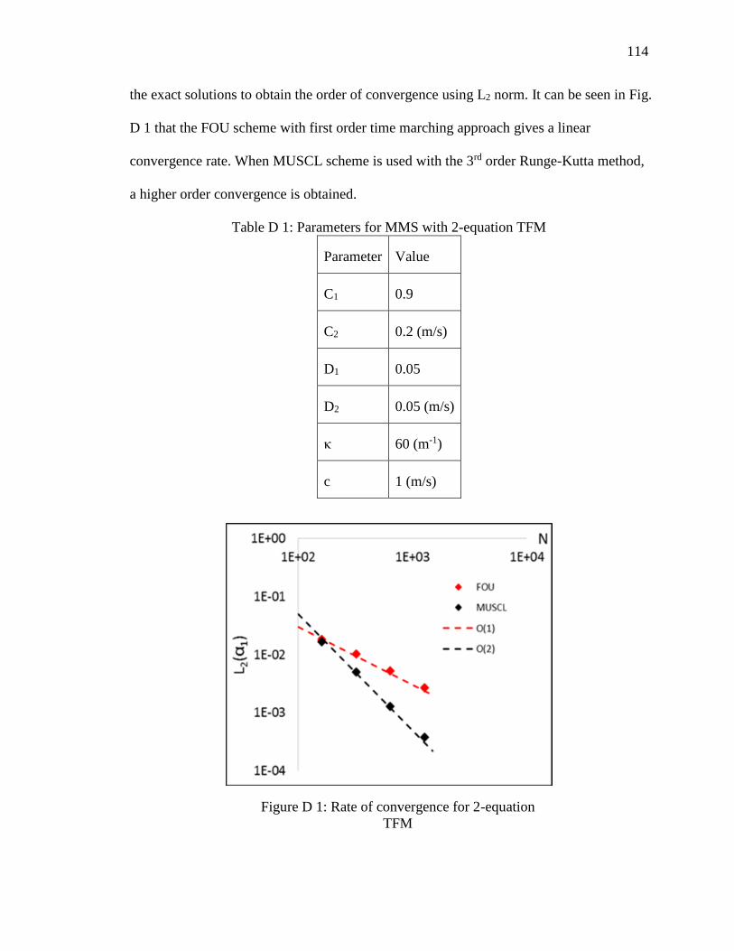
114
Figure D 1: Rate of convergence for 2-equation
TFM
the exact solutions to obtain the order of convergence using L2 norm. It can be seen in Fig.
D 1 that the FOU scheme with first order time marching approach gives a linear
convergence rate. When MUSCL scheme is used with the 3rd order Runge-Kutta method,
a higher order convergence is obtained.
Table D 1: Parameters for MMS with 2-equation TFM
Parameter Value
C1 0.9
C2 0.2 (m/s)
D1 0.05
D2 0.05 (m/s)
κ 60 (m-1)
c 1 (m/s)

115
The approach of verification and validation is extended to CFD analysis with the
commercial code ANSYS Fluent (version 15.0). Researchers in the past have been
successful in implementing MMS to verify the Navier Stokes solvers using the method of
manufactured solutions. This includes the work of Roy et al. [79], and Vedovoto et al.
[80]. Very little has been done for the case of MMS applied to TFM solvers. Choudhary
et al. [81] performed MMS for the TFM implemented in the commercial code MFIX.
In the present work, the verification procedure is performed on a 2-D domain for the
incompressible TFM. It was noted previously that for the case of single phase
incompressible flows, the velocity field chosen as an exact solution must be divergence
free, i.e., ∇. 𝑢 = 0. For two-phase flows, the analogous constraint would be a divergence
free volumetric flux, i.e., ∇. 𝑗 = 0. Similar to Vedovoto et al. [80], the initial conditions
are described for void fraction, x component velocity, y component velocity and pressure
given by,
��1 = 𝑢0𝑠𝑖𝑛2 (2𝜋
𝜆(𝑥 + 𝑦)) (D.9)
��1 = 𝑣0𝑐𝑜𝑠2 (2𝜋
𝜆(𝑥 + 𝑦)) (D.10)
𝑝 = 𝑝0 (𝑐𝑜𝑠 (2𝜋
𝜆(𝑥 + 𝑦)) − 1) (D.11)
��2 = 𝛼2,0 + 𝛿𝑐𝑜𝑠 (2𝜋
𝜆(𝑥 + 𝑦)) (D.12)
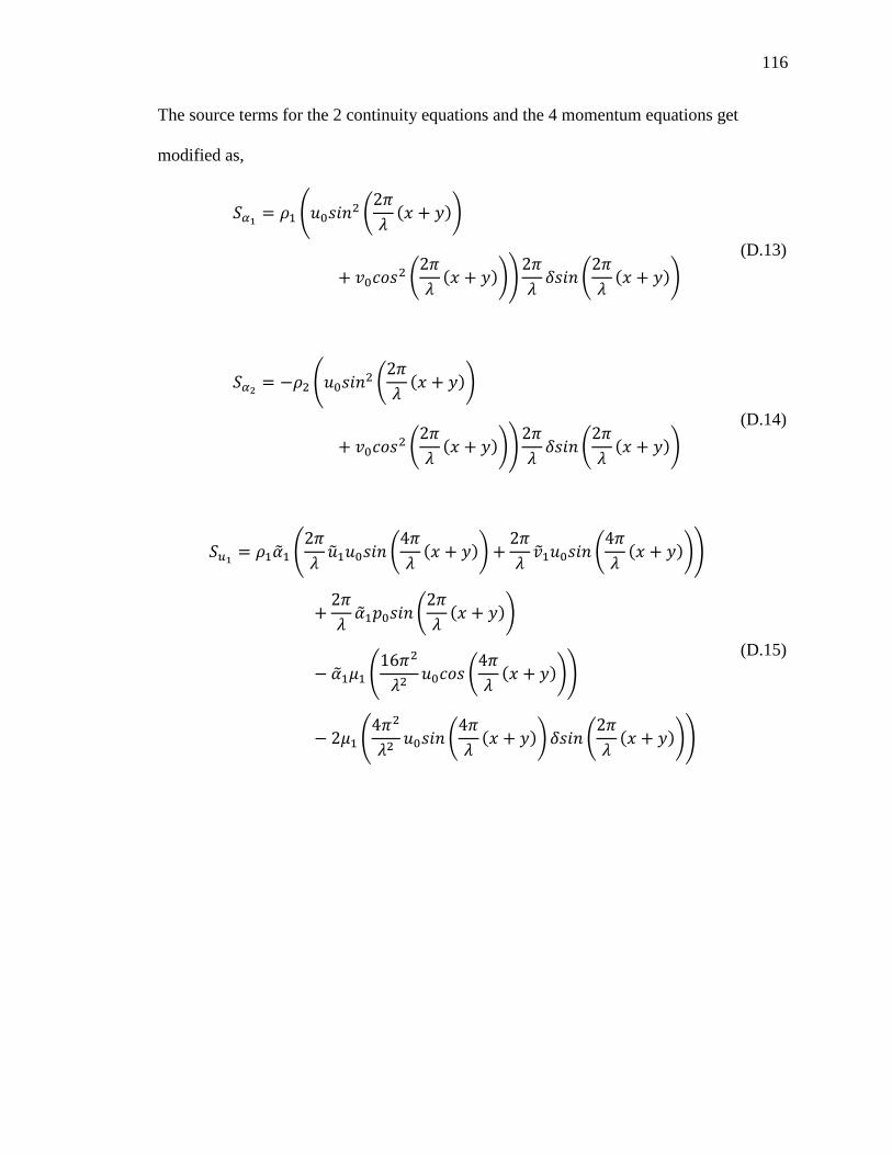
116
The source terms for the 2 continuity equations and the 4 momentum equations get
modified as,
𝑆𝛼1= 𝜌1 (𝑢0𝑠𝑖𝑛2 (
2𝜋
𝜆(𝑥 + 𝑦))
+ 𝑣0𝑐𝑜𝑠2 (2𝜋
𝜆(𝑥 + 𝑦)))
2𝜋
𝜆𝛿𝑠𝑖𝑛 (
2𝜋
𝜆(𝑥 + 𝑦))
(D.13)
𝑆𝛼2= −𝜌2 (𝑢0𝑠𝑖𝑛2 (
2𝜋
𝜆(𝑥 + 𝑦))
+ 𝑣0𝑐𝑜𝑠2 (2𝜋
𝜆(𝑥 + 𝑦)))
2𝜋
𝜆𝛿𝑠𝑖𝑛 (
2𝜋
𝜆(𝑥 + 𝑦))
(D.14)
𝑆𝑢1= 𝜌1��1 (
2𝜋
𝜆��1𝑢0𝑠𝑖𝑛 (
4𝜋
𝜆(𝑥 + 𝑦)) +
2𝜋
𝜆��1𝑢0𝑠𝑖𝑛 (
4𝜋
𝜆(𝑥 + 𝑦)))
+2𝜋
𝜆��1𝑝0𝑠𝑖𝑛 (
2𝜋
𝜆(𝑥 + 𝑦))
− ��1𝜇1 (16𝜋2
𝜆2𝑢0𝑐𝑜𝑠 (
4𝜋
𝜆(𝑥 + 𝑦)))
− 2𝜇1 (4𝜋2
𝜆2𝑢0𝑠𝑖𝑛 (
4𝜋
𝜆(𝑥 + 𝑦)) 𝛿𝑠𝑖𝑛 (
2𝜋
𝜆(𝑥 + 𝑦)))
(D.15)

117
𝑆𝑢2= 𝜌2��2 (
2𝜋
𝜆��2𝑢0𝑠𝑖𝑛 (
4𝜋
𝜆(𝑥 + 𝑦)) +
2𝜋
𝜆��2𝑢0𝑠𝑖𝑛 (
4𝜋
𝜆(𝑥 + 𝑦)))
+2𝜋
𝜆��2𝑝0𝑠𝑖𝑛 (
2𝜋
𝜆(𝑥 + 𝑦))
− ��2𝜇2 (16𝜋2
𝜆2𝑢0𝑐𝑜𝑠 (
4𝜋
𝜆(𝑥 + 𝑦)))
− 2𝜇2 (4𝜋2
𝜆2𝑢0𝑠𝑖𝑛 (
4𝜋
𝜆(𝑥 + 𝑦)) 𝛿𝑠𝑖𝑛 (
2𝜋
𝜆(𝑥 + 𝑦)))
(D.16)
𝑆𝑣1= 𝜌1��1 (
2𝜋
𝜆��1𝑣0𝑠𝑖𝑛 (
4𝜋
𝜆(𝑥 + 𝑦)) +
2𝜋
𝜆��1𝑣0𝑠𝑖𝑛 (
4𝜋
𝜆(𝑥 + 𝑦)))
+2𝜋
𝜆��1𝑝0𝑠𝑖𝑛 (
2𝜋
𝜆(𝑥 + 𝑦))
− ��1𝜇1 (16𝜋2
𝜆2𝑣0𝑐𝑜𝑠 (
4𝜋
𝜆(𝑥 + 𝑦)))
− 2𝜇1 (4𝜋2
𝜆2𝑣0𝑠𝑖𝑛 (
4𝜋
𝜆(𝑥 + 𝑦)) 𝛿𝑠𝑖𝑛 (
2𝜋
𝜆(𝑥 + 𝑦)))
(D.17)
𝑆𝑣2= 𝜌2��2 (
2𝜋
𝜆��2𝑣0𝑠𝑖𝑛 (
4𝜋
𝜆(𝑥 + 𝑦)) +
2𝜋
𝜆��2𝑣0𝑠𝑖𝑛 (
4𝜋
𝜆(𝑥 + 𝑦)))
+2𝜋
𝜆��2𝑝0𝑠𝑖𝑛 (
2𝜋
𝜆(𝑥 + 𝑦))
− ��2𝜇2 (16𝜋2
𝜆2𝑣0𝑐𝑜𝑠 (
4𝜋
𝜆(𝑥 + 𝑦)))
− 2𝜇2 (4𝜋2
𝜆2𝑣0𝑠𝑖𝑛 (
4𝜋
𝜆(𝑥 + 𝑦)) 𝛿𝑠𝑖𝑛 (
2𝜋
𝜆(𝑥 + 𝑦)))
(D.18)
A square domain 1 m by 1 m is chosen for the CFD calculations. Uniform grid with 80 x
80, 160 x 160, 320 x 320, and 640 x 640 nodes are chosen. The time step size is chosen

118
such that Δ𝑡 Δ𝑥⁄ = 0.1. The calculations are performed for 2s using QUICK scheme for
spatial discretization and second order implicit temporal scheme. Table D 2 summarizes
the parameters used for verifying the CFD TFM code (ANSYS Fluent 15.0). It can be
seen from Fig. D 2 that for the case of velocities, convergence with O(1.9) is obtained,
while for void fraction and pressure, convergence with O(1.5) is seen.
Table D 2: Parameters for MMS with CFD TFM
Parameter Value
u0 1 (ms-1)
v0 1 (ms-1)
p0 1 (Pa)
α2,0 0.05 ()
δ 0.01 ()
λ 0.1 (m)
μ1 1 (ms-2)
μ2 1 (ms-2)
ρ1 1 (kgm-3)
ρ2 1 (kgm-3)
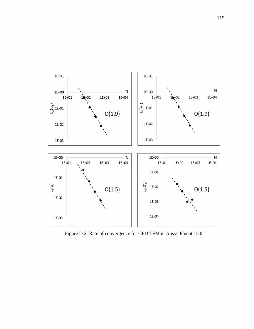
119
Figure D 2: Rate of convergence for CFD TFM in Ansys Fluent 15.0

120
REFERENCES

120
REFERENCES
[1] C. Pauchon and S. Banerjee, "Interphase Momentum Interaction Effects in the
Averaged Multifield Model, Part 1: Void Propagation in Bubbly Flows,"
International Journal of Multiphase Flow, vol. 12, pp. 559-573, 1986.
[2] M. Ishii, Thermo-fluid Dynamic Theory of Two-phase Flow, Paris: Eyrolles, 1975.
[3] P. Vernier and J. M. Delhaye, "General Two-phase Flow Equations Applied to the
Thermohydrodynamics of Boiling Nuclear Reactors," Energie Primaire, vol. 4,
1968.
[4] J. D. Ramshaw and J. A. Trapp, "Characteristics, Stability and Short-wavelength
Phenomenona in Two=phase Flow Equation Systems," Nuclear Science and
Engineering, vol. 66, pp. 93-102, 1978.
[5] R. W. Lyczkowski, D. Gidaspow, C. W. Solbrig and E. D. Hughes, "Characteristics
and Stability Analyses of Transient One-dimensional Two-phase Flow Equations
and Their Finite Difference Approximations," Nuclear Science and Engineering,
vol. 66, pp. 378-396, 1978.
121
[6] J. H. Stuhmiller, "The Influence of Interfacial Pressure Forces on the Character of
Two-phase Flow Model Equations," International Journal of Multiphase Flow, vol.
3, pp. 551-560, 1977.
[7] T. Haley, D. Drew and R. Lahey, "An analysis of the Eigenvalues of Bubbly Two-
phase Flows," Chemical Engineering Communications, vol. 106, pp. 93-117, 1991.
[8] J. W. Park, D. A. Drew and R. T. Lahey, "The Analysis of Void Wave Propagation
in Adiabatic in Adiabatic Monodispersed Bubbly Two-phase Flows Using an
Ensemble-averaged Two-fluid Model," International Journal of Multiphase Flow,
vol. 24, pp. 1205-1244, 1998.
[9] S. Ogawa, A. Umemura and N. Oshima, "On the Equations of Fully Fluidized
Granular Materials," Journal of Applied Mathematics and Physics, vol. 31, pp. 483-
493, 1980.
[10] S. B. Savage and D. J. Jeffrey, "The Stress Tensor in a Granular Flow at High Shear
Rates," Journal of Fluid Mechanics, vol. 110, pp. 255-272, 1981.
[11] N. F. Carnahan and K. E. Starling, "Equations of State for Non-attracting Rigid
Spheres," Journal of Chemical Physics, vol. 51, pp. 635-636, 1969.
[12] C. K. Lun, S. B. Savage, D. J. Jeffrey and N. Chepurniy, "Kinetic Theories for
Granular Flow: Inelastic Particles in Couette Flow and Slightly Inelastic Particles in
a General Flowfield," Journal of Fluid Mechanics, vol. 140, pp. 223-256, 1984.
122
[13] C. K. Lun and S. B. Savage, "The Effects of an Impact Velocity Dependent
Coefficient of Restitution on Stresses Developed by Sheared Granular Materials,"
Acta Mechanica, vol. 63, pp. 15-44, 1986.
[14] A. Boelle, G. Balzer and O. Simonin, "Second-order Prediction of the Particle-phase
Stress Tensor of Inelastic Spheres in Simple Shear Dense Suspensions," in Gas
Particle Flows, ASME FED, 1995.
[15] A. Alajbegovic, D. A. Drew and R. T. Lahey Jr., "An Analysis of Phase Distribution
and Turbulence in Dispersed Particle/liquid Flows," Chemical Engineering
Communications, vol. 174, pp. 85-133, 1999.
[16] A. Alajbegovic, F. Assad , F. Bonetto and R. T. Lahey, "Phase Distribution and
Turbulence Structure for Solid/Fluid Upflow in a Pipe," International Journal of
Multiphase Flow, vol. 20, pp. 453-479, 1994.
[17] B. N. Reddy Vanga, Experimental Investigation and Two-Fluid Model Large Eddy
Simulations of Re-circulating Turbulent Flow in Bubble Columns, West Lafayette,
Indiana: Purdue University, 2004.
[18] N. G. Deen, T. Solberg and B. H. Hjertager, "Large Eddy Simulation of the Gas-
liquid Flow in a Square Cross-sectioned BubbleColumn," Chemical Engineering
Science, vol. 56, pp. 6341-6349, 2001.
[19] D. Lakehal, B. L. Smith and M. Milelli, "Large Eddy Simulation of Bubbly
Turbulent Shear Flows," Jouornal of Turbulence, vol. 3, 2002.

123
[20] M. Milelli, A Numerical Analysis of Confined Turbulent Bubble Plumes, Zurich:
Swiss Federal Institute of Technology, 2002.
[21] D. Zhang, N. G. Deen and J. A. Kuipers, "Numerical Simulation of the Dynamic
Flow Behavior in a Bubble Column: A study of Closures for Turbulence and
Interface Forces," Chemical Engineering Science, vol. 61, pp. 7593-7608, 2006.
[22] J. Smagorinsky, "General Circulation Experiments with the Primitive Equations I.
The Basic Experiment," Monthly Weather Review, vol. 91, pp. 99-163, 1963.
[23] M. T. Dhotre, B. Niceno and B. L. Smith, "Large Eddy Simulation of a Bubble
Column Using Dynamic Sub-grid Scale Model," Chemical Engineering Journal,
vol. 136, pp. 337-348, 2008.
[24] B. Niceno, M. T. Dhotre and N. G. Deen, "One-equation Sub-grid Scale (SGS)
Modelling for Euler-Euler Large Eddy Simulation (EELES) of Dispersed Bubbly
Flow," Chemical Engineering Science, vol. 63, pp. 3923-3931, 2008.
[25] S. Ojima, K. Hayashi, S. Hosokawa and A. Tomiyama, "Distributions of Void
Fraction and Liquid Velocity in Air-water Bubble Column," International Journal of
Multiphase Flow, vol. 67, pp. 111-121, 2014.
[26] J. L. Marie, E. Moursali and S. Tran-Cong, "Similarity Law and Turbulence
Intensity Profiles in a Bubbly Boundary Layer," International Journal of Multiphae
Flow, vol. 23, pp. 227-247, 1997.

124
[27] A. E. Larreteguy, D. A. Drew and R. T. Lahey Jr., "A Particle Center-averaged Two-
fluid Model for Wall-bounded bubbly Flows," in ASME Fluid Engineering Division
Summer Meeting, Montreal, 2002.
[28] F. J. Moraga, A. E. Larreteguy, D. A. Drew and R. T. Lahey Jr., "A Center-averaged
Two-fluid Model for Wall-bounded Bubbly Flows," Computers and Fluids, vol. 35,
pp. 429-461, 2006.
[29] N. Zuber and J. A. Findlay, "Average Volumetric Concentration in Two-phase Flow
Systems," Journal of Heat Transfer, vol. 87, pp. 453-468, 1965.
[30] M. Ishii and T. C. Chawla, "Local Drag Laws in Dispersed Two-phase Flow," ANL,
Argonne, 1979.
[31] T. R. Auton, "The Lift Force on a Spherical Body in a Rotational Flow," Journal of
Fluid Mechanics, vol. 183, pp. 199-218, 1987.
[32] D. A. Drew and R. T. Lahey Jr., "The Virtual Mass and Lift Force on a Sphere in
Rotating and Straining Inviscid Fluid," International Journal of Multiphase Flow,
vol. 13, no. 1, pp. 113-121, 1987.
[33] A. Tomiyama, H. Tarnai, I. Zun and S. Hosokama, "Transverse Migration of Single
Bubbles in Simple Shear Flow," Chemical Science and Engineering, vol. 57, pp.
1849-1858, 2002.
[34] T. Frank, J. M. Shi and A. D. Burns, "Validation of Eulerian Multiphase Flow
Models for Nuclear Safety Applications," in Third International Symposium on Two-
phase Flow Modeling and Experimentation, Pisa, 2004.
125
[35] E. Moursali, J. L. Marie and J. Bataille, "An Upward Turbulent Bubbly Boundary
Layer Along a Vertical Flat Plate," International Journal of Multiphase Flow, vol.
21, no. 1, pp. 107-117, 1995.
[36] M. Lopez de Bertodano, "Turbulent Bubbly Two-phase Flow in a Triangular Duct,"
Troy, 1992.
[37] S. P. Antal, R. T. Lahey and J. E. Flaherty, "Analysis of Phase distribution in Fully
Developed Laminar Bubbly Two-phase Flow," International Journal of Multiphae
Flow, vol. 17, pp. 635-652, 1991.
[38] H. Lamb, Hydrodynamics, New York: Dover, 1932.
[39] N. Zuber, "On the Dispersed Two-phase Flow in the Laminar Flow Regime,"
Chemical Engineering Science, vol. 19, pp. 897-917, 1964.
[40] D. A. Drew and S. L. Passman, Theory of Multicomponent Fluids, New York:
Springer-Verlag, 1998.
[41] M. Lopez de Bertodano, R. T. Lahey Jr. and O. C. Jones, "Development of a k-
epsilon Model for Bubbly Two-phase Flow," Journal of Fluids Engineering, vol.
116, pp. 128-134, 1994.
[42] B. E. Launder and D. B. Spalding, "The Numerical Computation of Turbulent
Flows," Computer Methods in Applied Mechanics and Engineering, vol. 3, pp. 269-
289, 1974.
[43] Y. Sato and K. Sekoguchi, "Liquid Velocity Distribution in Two-phase Bubble
Flow," International Journal of Multiphase Flow, vol. 2, pp. 79-95, 1975.

126
[44] M. Ishii and T. Hibiki, Thermo-fluid Dynamics of Two-phase Flow, 2 ed., New
York: Springer, 2011.
[45] M. Lopez de Bertodano, W. Fullmer and A. Vaidheeswaran, "One-dimensional
Two-equation Two-fluid Model Stability," Multiphase Science and Technology, vol.
25, pp. 133-167, 2013.
[46] G. B. Whitham, Linear and Non-linear Waves, New York: Wiley, 1975.
[47] A. Matuszkiewicz, J. C. Flamand and J. A. Boure, "The Bubble-slug Flow Pattern
Transition and Instabilities of Void Fraction Waves," International Journal of
Multiphase Flow, vol. 2, pp. 199-217, 1987.
[48] J. W. Park, D. A. Drew and R. T. Lahey Jr., "The Measuement of Void Waves in
bubbly Two-phase Flows," Nuclear Engineering and Design, vol. 149, pp. 37-52,
1994.
[49] H. Cheng, J. H. Hills and B. J. Azzopardi, "Effects of Initial Bubble Size on Flow
Pattern Transition in a 28.9 mm Diameter Column," International Journal of
Multiphase Flow, vol. 28, pp. 1047-1062, 2002.
[50] A. Zaruba, E. Krepper, H.-M. Prasser and E. Schliecher, "Measurement of Bubble
Velocity Profiles and Turbulent Diffusion Coefficients of the Gaseous Phase in
Rectangular Bubble Column Using Image Processing," Experimental Thermal and
Fluid Science, vol. 29, pp. 851-860, 2005.
[51] S. Chapman and T. G. Cowling, The Mathematical Theory of Non-uniform Gases,
London: Cambridge University Press, 1970.
127
[52] H. K. Kytomaa and C. E. Brennen, "Small Amplitude Kinematic Wave Propagation
in Two-component Media," International Journal of Multiphase Flow, vol. 17, no.
1, pp. 13-26, 1991.
[53] H. Pokharna, M. Mori and V. H. Ransom, "Regularization of Two-phase Flow
Models: A Comparison of Numerical and Differential Approaches," Journal of
Computational Physics, vol. 134, pp. 282-295, 1997.
[54] W. D. Fullmer, M. Lopez de Bertodano, M. Chen and A. Clausse, "Analysis of
Stability, Verification and Chaos with the Kreiss-Ystrom Equations," Applied
Mathematics and Computation, vol. 248, pp. 28-46, 2014.
[55] N. P. Waterson and H. Deconinck, "Desing Principles for Bounded Higher-order
Convection Schemes - A Unified Approach," Journal of Computational Physics,
vol. 224, pp. 182-207, 2007.
[56] P. L. Roe, "Characteristic-based Schemes for the Euler Equations," Annual Review
of Fluid Mechanics, vol. 18, pp. 337-365, 1986.
[57] B. van Leer, "Towards the Ultimate Conservative Difference Scheme . V. A Second-
order Sequel to Godunov's Method," Journal of Computational Physics, vol. 32, no.
1, pp. 101-136, 1979.
[58] P. H. Gaskell and A. K. Lau, "Curvature-compensated Convective Transport:
SMART, a New Boundedness-preserving Transport Algorithm," International
Journal of Numerical Methods in Fluids, vol. 8, pp. 617-641, 1988.

128
[59] S. Gottlieb and C. W. Shu, "Total Variation Diminishing Runge-Kutta Schemes,"
Mathematics of Computation, vol. 67, pp. 73-85, 1998.
[60] C. T. Crowe, M. P. Sharma and D. E. Stock, "The Particle Source-in-cell (PSI-
CELL) for Gas Droplet Flows," Journal of Fluids Engineering, vol. 99, pp. 325-331,
1977.
[61] J. S. Shuen, L. D. Chen and G. M. Faeth, "Evaluation of a Stochastic Model of
Particle Dispersion in a Turbulent Round Jet," AIChE, vol. 29, pp. 167-170, 1983.
[62] A. A. Mostafa and H. C. Mongia, "On the Interaction of Particles and Turbulent
Fluid Dlow," International Journal of Heat and Mass Transfer, vol. 31, pp. 2063-
2075, 1988.
[63] J. A. Trapp and G. A. Mortensen, "A Discrete Particle Model for Bubble-slug Two-
phase Flows," Journal of Computational Physics, vol. 107, pp. 367-377, 1993.
[64] K. C. Chang and W. J. Wu, "Sensitivity Study on Monte Carlo Solution Procedure
of Two-phase Turbulent flow," Numerical Heat Transfer, vol. 25, pp. 223-244,
1994.
[65] M. Sommerfeld, "Analysis of Collision Effects for Turbulent Gas-particle Flow in a
Horizontal Channel: Part I. Particle Transport," International Journal of Multiphase
Flows, vol. 29, pp. 675-699, 2003.
[66] A. W. Vreman, "Turbulence Characteristics of Particle-laden Pipe Flow," Journal of
Fluid Mechanics, vol. 584, pp. 235-279, 2007.

129
[67] M. Mando and Y. Chungen, "Euler-Lagrangian Simulation of Gas-solid Pipe Flow
with Smooth and rough Wall Boundary Conditions," Powder Technology, vol. 225,
pp. 32-42, 2012.
[68] ANSYS CFX 15.0, CFX Solver Theory Guide, 2013.
[69] T. J. Barth and D. C. Jespersen, "The Design and Application of Upqind Schemes on
Unstructured Meshes," in AIAA, Reno, 1989.
[70] B. P. Leonard, "A Stable and Accurate Convective Modelling Procedure Based on
Quadratic Upstream Interpolation," Computer Methods in Applied Mechanics and
Engineering, vol. 19, pp. 59-98, 1979.
[71] ANSYS Fluent 15.0, Fluent Theory guide, 2013.
[72] B. A. Kader, "Temperature and Concentration Profiles in Fully Turbulent Boundary
Layers," International Journal of Heat and Mass Transfer, vol. 24, no. 9, pp. 1541-
1544, 1981.
[73] M. Lopez de Bertodano, X. Sun and J. Buchanan, "A Three-field Two-fluid CFD
Model with a Laterall Displacement Force for Cap Bubble Regime in a Duct," in
Sixth International Conference on Multiphase Flow, Leipzig, 2007.
[74] D. Prabhudharwadkar, A. Vaidheeswaran, M. Lopez de Bertodano, J. Buchanan and
P. Guilbert, "Two-fluid CFD Simulations of Cap Bubble Flow Using the Two-group
Interfacial Area Transport Equations," Journal of Computational Multiphase Flows,
vol. 4, pp. 363-374, 2012.

130
[75] X. Sun, "Two-group Interfacial Area Transport Equation for a Confined Test
Section," West Lafayette, 2001.
[76] R. E. Henry, M. A. Grolmes and H. K. Fauske, "Pressure-pulse Propagation in Two-
phase and Two-componenet Mixtures," Argonne, 1971.
[77] V. J. Dejong and J. C. Firey, "Effect of Slip and Phase Change on Sound Velocity in
Steam-water Mixtures and the Relation to Critical Flow," I & EC Process Design
and Development, vol. 7, pp. 454-463, 1968.
[78] P. J. Roache, "Code Verification by the Method of Manufactured Solutions,"
Journal of Fluids Engineering, vol. 124, pp. 4-10, 2002.
[79] C. J. Roy, C. C. Nelson, T. M. Smith and C. C. Ober, "Verification of Euler/Navier-
Stokes Codes Using the Method of Manufactured Solutions," International Journal
for Numerical Methods in Fluids, vol. 44, pp. 599-620, 2004.
[80] J. M. Vedovoto, A. Neto, A. Mura and L. da Silva, "Application of the Method of
Manufactured Solutions to the Verification of a Pressure-based Finite-volume
Numerical Scheme," Computers and Fluids, vol. 51, pp. 85-99, 2011.
[81] A. Choudhary, C. J. Roy, J. F. Dietiker, M. Shahnam and R. Garg, "Code
Verification for Multiphse Flows Using the Method of Manufactured Solutions," in
ASME Fluids Engineering Division, Chicago, 2014.
[82] J. L. Guermond and J. Shen, "A New Class of Truly Consistent Splitting Schemes
for Incompressible Flows," Journal of Computational Physics, vol. 192, pp. 262-
276, 2003.

131
VITA

131
VITA
Avinash Vaidheeswaran was born in Chennai, India on December 6, 1987. He
received his high school education from DAV senior secondary school, Chennai. He
received the merit certificate for being placed in top 0.1% in India in Physics high school
final examination. He pursued his Bachelors studies from 2005 – 2009 at the Department
of Mechanical Engineering at National Institute of Technology, Trichy, India. He served
as a Research Assistant at the Department of Mechanical Engineering, IIT Madras to Dr.
Raghavan Vasudevan and worked on droplet combustion experiments. He also worked
under the guidance of Dr. Sunetra Sarkar at the Department of Aerospace Engineering,
IIT Madras on modeling the insect wing flapping mechanism.
He began his doctoral studies at Purdue University under the supervision of Dr.
Martin Lopez de Bertodano. He received a five-year Lynn fellowship from the graduate
school. During his dissertation work, he has collaborated with Bechtel Marine Propulsion
Corporation and Ansys UK in developing CFD two-fluid model. His research interests
include two-phase flows, stability analysis, turbulence, CFD, and boiling heat transfer.
Upon completion of his doctoral studies, he will continue as a postdoctoral research
associate at Purdue University with Dr. Martin Lopez de Bertodano.


![GLOBAL WELL-POSEDNESS OF THE MAXWELL-KLEIN-GORDON … · arxiv:0910.1850v2 [math.ap] 12 aug 2010 global well-posedness of the maxwell-klein-gordon equation below the energy norm markus](https://img.pdfslide.us/doc/110x75/5b82ba157f8b9a934f8ba1e3/global-well-posedness-of-the-maxwell-klein-gordon-arxiv09101850v2-mathap.jpg)