Research Article The Well-Posedness and Stability Analysis of a …downloads.hindawi.com/journals/jam/2013/131076.pdf · 2019-07-31 · Research Article The Well-Posedness and Stability

Hindawi Publishing CorporationJournal of Applied MathematicsVolume 2013 Article ID 131076 9 pageshttpdxdoiorg1011552013131076

Research ArticleThe Well-Posedness and Stability Analysis ofa Computer Series System

Xing Qiao1 Dan Ma1 Fu Zheng2 and Guangtian Zhu3

1 School of Mathematical Science Daqing Normal University Daqing 163712 China2Department of Mathematics Bohai University Jinzhou 121013 China3 Academy of Mathematics and System Sciences CAS Beijing 100080 China

Correspondence should be addressed to Xing Qiao xiaoqiao1502163com

Received 13 August 2012 Accepted 2 April 2013

Academic Editor Vu Phat

Copyright copy 2013 Xing Qiao et al This is an open access article distributed under the Creative Commons Attribution Licensewhich permits unrestricted use distribution and reproduction in any medium provided the original work is properly cited

A repairable computer system model which consists of hardware and software in series is established in this paper This study isdevoted to discussing the unique existence of the solution and the stability of the studied system In view of 119888

0semigroup theory

we prove the existence of a unique nonnegative solution of the system Then by analyzing the spectra distribution of the systemoperator we deduce that the transient solution of the system strongly converges to the nonnegative steady-state solution which isthe eigenvector corresponding to eigenvalue 0 of the system operator Finally some reliability indices of the system are provided atthe end of the paper with a new method

1 Introduction

With the development of the modern technology and theextensive use of the electronic products the reliability prob-lem of the repairable systems has become a hot topic It is wellknown that the reliability of a system is an important conceptin engineering The high degree of reliability is usuallyachieved by introducing redundancy or repairman (eg [1ndash4]) or applying preventive maintenance (eg [5 6]) optimalinspection plans (eg [7ndash9]) or optimal replacement policy(eg [10]) The aim is to increase the performance of thesystem by reducing the downtime or the maintenance andinspection cost of the system

In the general reliability analysis of the computer systemhowever because of different characteristics of the hardwareand software we cannot simply take the hardware and soft-ware as a unit or two different types of units [9] Then it israre to analyze synthetically [11]With the passage of the usingtime and the number of failures increasing the reliability ofthe hardware would descend and the repair time would belonger [12] During the software debugging and testing stagesas the failures occur potential software error is discoveredand corrected constantly which make the software reliabilitygrow [13] Since the hardware failure or software failure

leads to the whole computer system failure the computersystem can be formulated as a series system with hardwareand software (namely hardware and software in series)Thereare someobstacles to overcome to obtain themain result sinceour model is more complicated than that of [11ndash13]

In this paper we study a repairable computer systemwhich is composed of hardware and software in series Theunique existence of the system solution is obtained by using1198880semigroup theory The exponential stability of the system

is further achieved by analyzing the spectrum distribution ofthe system operator given by (2)ndash(4) which shows that thesolution to the system (2)ndash(4) is exponentially stableThuswenot only provide strict theoretical foundation for reliabilitystudy but also make it more valuable in practice

The remainder of the paper is organized as follows InSection 2 we formulate themathematicalmodel of the systemwith concerned notations in Section 31 we show the uniqueexistence of the dynamic solution of the system In Section 32we study the unique existence of the solution of the abstractCauchy problem corresponding to the system and presenta detailed spectral analysis of the system operator somesteady-state reliability indices of the system are presented inSection 4 and Section 5 concludes the paper

2 Journal of Applied Mathematics

2 Mathematical Model Formulation

In the reliability analysis of repair system it is usuallyassumed that the repaired units which compose system areas good as new and the failed units are repaired immediatelyHowever in reality it is usually not the case In real life it ispossible that the reliability reduces after the software failureeach time That is the condition 119865

(119899)

119878(119905) = 119865

119878(119886119899minus1

119905) = 1minus

119890minus119886119899minus1

120582119904119905 119905 ge 0 120582

119904gt 0 and the coefficient 119886 gt 1 With

the number of repair times increasing the failure rate isincreasing gradually In view of the aging and accumulativewear the repair time will become longer and longer andtend towards infinity that is the system is nonrepairableTherefore we first suppose that the software is overhauled(replaced) to be as good as new after the (119873 minus 1)th minimalrepair and studying the number of minimal repair beforeoverhaul repair is more appropriate And we will also discusshow its reliability will be affected by the number of minimalrepair and overhaul In [14] the author supposed that thesoftware cannot be repaired as good as new and utilized thegeometric process and supplementary variable technique toanalyze the system reliability However the life and repairtimes of the hardware and software are supposed to followexponential distribution In this paper under assumptionthat the life time of the hardware and software follows expo-nential distribution and repair time is subject to the generaldistribution we set up amathematicalmodel of the repairablecomputer system by the supplementary variable methodwhich is composed of the hardware and software in seriesThe hardware is repaired to be as good as new the softwareis repaired periodically and restored software life decreasesAfter a period of time an overhaul makes it as a new one

The system model is formulated specifically as follows

(i) The computer system is composed of hardware119867 andsoftware 119878 in series

(ii) The distribution function of the life time 119883119867

ofhardware119867 is 119865

119867(119905) = 1 minus 119890

minus120582ℎ119905 119905 ge 0 120582

ℎgt 0

(iii) The distribution function of the life time119883(119899)119878

of soft-ware 119878 during its 119899th period (eg the time betweenthe completion of its (119899 minus 1)th repair and that of the119899th repair) is 119865119899

119878(119905) = 119865

119878(119886119899minus1

119905) = 1 minus 119890minus119886119899minus1

120582119904119905 119905 ge 0

120582119904gt 0 119886 gt 1 119899 = 1 2 119873

(iv) Let 1198841be the repair time of hardware119867 119884

2the repair

time of software 119878 after its 119899th failure (119899 = 1 2 119873minus

1) and 1198843the repair time of software 119878 after its 119899th

failure respectively Their distribution functions are119866119895(119905) = int

119905

0119892119895(119909)119889119909 = 1minus119890

minusint119905

0

120583119895(119909)119889119909 and119864[119884

119895] = 1120583

119895

119895 = 1 2 3 where 1205833(119909) gt 120583

2(119909) for all 119909 ge 0

(v) The hardware 119867 is repaired as good as new Thesoftware 119878 is performed by a minimal repair (eg amaintenance action performed on a failed system bywhich its survival time is decreasing) during its 119899th(119899 = 1 2 119873 minus 1) period and an overhaul repair(eg a maintenance action performed on a failedsystem by which it is repaired as good as new) during

its 119873th period The above stochastic variables areindependent of each other

Let 119873(119905) be the system state at time 119905 and assume all thepossible states as below

0119894 (119894 = 1 2 119873) the system is working1119894 (119894 = 1 2 119873) the system is failed because the failure

hardware119867 is being repaired in the 119894th time2119894 (119894 = 1 2 119873) the system has in failure state because

the failure software 119878 is being repaired minimally in the119894th time (119894 = 1 2 119873 minus 1) and the software 119878 is beingoverhauled in the119873th time

Then the system state space is 119864 = 0119894 1119894 2119894 (119894 =

1 2 119873) in which the working state space is 119882 = 0119894

(119894 = 1 2 119873) and the failure state space is 119865 = 1119894 2119894

(119894 = 1 2 119873)When 119873(119905) = 119895119894 (119895 = 0 1 2 119894 = 1 2 119873) supple-

ment variable 119884119895(119905) (119895 = 1 2 3) which denotes the elapsed

repair time of hardware 119867 the elapsed minimal repairtime of software 119878 and its elapsed overhaul time at time 119905respectively then 119873(119905) 119884

119895(119905) constitutes a matrix Markov

process whose state probabilities are defined as follows

1198750119894 (

119905) = 119875 119873 (119905) = 0119894 119894 = 1 2 119873

1198751119894 (

119909 119905) = 119875 119909 lt 1198841 (

119905) le 119909 + 119889119909119873 (119905) = 1119894

119894 = 1 2 119873

1198752119894(119909 119905) = 119875 119909 lt 119884

2(119905) le 119909 + 119889119909119873 (119905) = 2119894

119894 = 1 2 119873 minus 1

1198752119873

(119909 119905) = 119875 119909 lt 1198843(119905) le 119909 + 119889119909119873 (119905) = 2119873

(1)

Then by using the method of probability analysis the systemunder consideration can be formulated as the following equa-tions

11988911987501 (

119905)

119889119905

= minus (120582ℎ+ 120582119904) 11987501 (

119905) + int

infin

0

11987511 (

119909 119905) 1205831 (119909) 119889119909

+ int

infin

0

1198752119873 (

119909 119905) 1205833 (119909) 119889119909

1198891198750119894(119905)

119889119905

= minus (120582ℎ+ 119886119894minus1

120582119904) 1198750119894(119905) + int

infin

0

1198751119894(119909 119905) 120583

1(119909) 119889119909

+ int

infin

0

1198752(119894minus1)

(119909 119905) 1205832(119909) 119889119909

119894 = 2 3 119873

1205971198751119894 (

119909 119905)

120597119909

+

1205971198751119894 (

119909 119905)

120597119905

= minus1205831 (

119909) 1198751119894 (119909 119905)

119894 = 1 2 119873

1205971198752119894(119909 119905)

120597119909

+

1205971198752119894(119909 119905)

120597119905

= minus1205832(119909) 1198752119894(119909 119905)

119894 = 1 2 119873 minus 1

1205971198752119873

(119909 119905)

120597119909

+

1205971198752119873

(119909 119905)

120597119905

= minus1205833(119909) 1198752119873

(119909 119905)

(2)

Journal of Applied Mathematics 3

The boundary conditions are1198751119894 (

0 119905) = 120582ℎ1198750119894 (

119905) 119894 = 1 2 119873

1198752119894 (

0 119905) = 119886119894minus1

1205821199041198750119894 (

119905) 119894 = 1 2 119873

(3)

The initial conditions are11987501

(0) = 1 and the others are equal to 0 (4)Taking into account the practical backgroundwe assume that

0 lt 119870 = sup119909isin[0infin)

120583119895(119909) lt infin

int

119879

0

120583119895(119909) 119889119909 lt infin 0 lt 119879 lt infin

int

infin

0

120583119895 (119909) 119889119909 = infin 119895 = 1 2 3

(5)

And then we may know that many repairsservices aredone periodically in practice So we can suppose that themean of repairservice rate exists and does not equal to 0([15 16])

0 lt 120583119895= lim119909rarrinfin

1

119909

int

119909

0

120583119895 (120591) 119889120591 lt infin 119895 = 1 2 3 (6)

3 Stability Analysis

In this section we firstly study the unique existence of theclassical solution of the system by pure analysis method inSection 31 In Section 32 we will formulate the problem intoa suitable Banach space Then we explain that the system hasa unique generalized solution and it is just the classical onewhen 119905 gt 0 We also carry out a detailed spectral analysis ofthe system operator119860+119864 Finally the exponential stability ofthe system can be readily achieved

31 Unique Existence of the Classical Solution

Theorem 1 The system (2)ndash(4) has a unique nonnegativesolution in 119862[0 119879] for any 119879 gt 0

Proof Solving (2)ndash(4) with the method in [17] one gets

11987501 (

119905) = 119890minus1205871119905+ int

infin

0

11989611

(119905 minus 120578) 11987511

(0 120578) 119889120578

+ int

infin

0

1198962119873

(119905 minus 120578) 1198752119873

(0 120578) 119889120578

1198750119894(119905) = 119890

minus120587119894119905+ int

infin

0

1198961119894(119905 minus 120578) 119875

1119894(0 120578) 119889120578

+ int

infin

0

1198962(119894minus1)

(119905 minus 120578) 1198752(119894minus1)

(0 120578) 119889120578

119894 = 2 3 119873

11987511

(0 119905) = 120582ℎ(119890minus1205871119905+ int

infin

0

11989611

(119905 minus 120578) 11987511

(0 120578) 119889120578

+int

infin

0

1198962119873

(119905 minus 120578) 1198752119873

(0 120578) 119889120578)

1198751119894 (

0 119905) = 120582ℎ(119890minus120587119894119905+ int

infin

0

1198961119894(119905 minus 120578) 119875

1119894(0 120578) 119889120578

+int

infin

0

1198962(119894minus1)

(119905 minus 120578) 1198752(119894minus1)

(0 120578) 119889120578)

119894 = 2 3 119873

11987521 (

0 119905) = 120582119904(119890minus1205871119905+ int

infin

0

11989611

(119905 minus 120578) 11987511

(0 120578) 119889120578

+int

infin

0

1198962119873

(119905 minus 120578) 1198752119873

(0 120578) 119889120578)

1198752119894 (

0 119905) = 119886119894minus1

120582119904(119890minus120587119894119905+ int

infin

0

1198961119894(119905 minus 120578) 119875

1119894(0 120578) 119889120578

+int

infin

0

1198962(119894minus1)

(119905 minus 120578) 1198752(119894minus1)

(0 120578) 119889120578)

119894 = 2 3 119873

(7)

where

120587119894= 120582ℎ+ 119886119894minus1

120582119904

1198961119894(119905 minus 120578) = int

119905minus120578

0

119890minus120587119894(119905minus120578)120587

119894Vminusint

V

0

1205831(120591)119889120591

1205831(V) 119889V

119894 = 1 2 119873

1198962119894(119905 minus 120578) = int

119905minus120578

0

119890minus120587119894+1(119905minus120578)120587

119894+1Vminusint

V

0

1205832(120591)119889120591

1205832(V) 119889V

119894 = 1 2 119873 minus 1

1198962119873

(119905 minus 120578) = int

119905minus120578

0

119890minus1205871(119905minus120578)120587

1Vminusint

V

0

1205833(120591)119889120591

1205833(V) 119889V

(8)

With the help of (7) we can get the following convolu-tion-type integral equation

119875 (119905) = 119865 (119905) + int

119905

0

119870(119905 minus 120578) 119875 (120578) 119889120578 (9)

where119875 (119905) = (119875

01(119905) 119875

0119873(119905) 11987511

(0 119905) 1198751119873

(0 119905)

11987521 (

0 119905) 1198752119873 (0 119905))119879

119865 (119905) = (119891 (119905) 120582ℎ119891 (119905) 120582119904

(119890minus1205871119905 119886119890minus1205872119905 119886

119873minus1119890minus120587119873119905)

119879

119891 (119905) = (119890minus1205871119905 119890minus1205872119905 119890

minus120587119873119905)

119870 (119905 minus 120578) = (

119874119899times119899

11987011

(119905 minus 120578) 11987012

(119905 minus 120578)

119874119899times119899

11987021

(119905 minus 120578) 11987022

(119905 minus 120578)

119874119899times119899

11987031

(119905 minus 120578) 11987032

(119905 minus 120578)

)

11987012

(119905 minus 120578)

= (

0 sdot sdot sdot 0 1198962119873

(119905 minus 120578)

11989621

(119905 minus 120578) sdot sdot sdot 0 0

d

0 sdot sdot sdot 119896

2(119873minus1)(119905 minus 120578) 0

)

119899times119899


11987022

(119905 minus 120578) = 120582ℎ11987012

(119905 minus 120578)

11987032

(119905 minus 120578)

= (

0 sdot sdot sdot 0 1205821199041198962119873(119905 minus 120578)

11988612058211990411989621(119905 minus 120578) sdot sdot sdot 0 0

d


119873minus11205821199041198962(119873minus1)(119905 minus 120578) 0

)

119899times119899

11987011

(119905 minus 120578) = diag (11989611

(119905 minus 120578) 11989611

(119905 minus 120578)

11989611

(119905 minus 120578))119899times119899

11987021

(119905 minus 120578) = diag (120582ℎ11989611

(119905 minus 120578) 120582ℎ11989611

(119905 minus 120578)

120582ℎ11989611

(119905 minus 120578))119899times119899

11987031

(119905 minus 120578) = diag (12058211990411989611

(119905 minus 120578) 11988612058211990411989611

(119905 minus 120578)

119886119873minus1

12058211990411989611

(119905 minus 120578))119899times119899

(10)

It is clear that the unique existence of the nonnegativesolution of the system (2)ndash(4) is equal to that of the convo-lution-type integral equation (9) Since for any 119879 gt 0 eachcoordinate of 119865(119905) and 119870(119905 minus 120578) is nonnegatively boundedfunction and is absolutely integrable in119862[0 119879] we can obtainthat the convolution-type integral equation (9) has a uniquenonnegative solution in 119862[0 119879] by using the related theoryin integral equation For this reason the system (2)ndash(4) hasa unique nonnegative solution in 119862[0 119879] for any 119879 gt 0 Theproof is complete

32 Exponential Stability In this subsection in order tofurther study the properties of the studied system we willformulate the problem into a suitable Banach space Thenwe study the unique existence of its solution and explain theexponential stability of the system by analyzing the spectrumdistribution of the system operator in detail

Firstly let the state space 119883 be

119883 = 119875 isin 119877119899times (1198711(119877+) times 1198711(119877+))

119899

| 119875

=

10038161003816100381610038161003816119875010038161003816100381610038161003816+

2

sum

119894=1

1003817100381710038171003817100381711987511989410038171003817100381710038171003817lt infin

(11)

where

119875 = (1198750 1198751(119909) 119875

2(119909))

1198750= (11987501 11987502 119875

0119873)119879

1198751(119909) = (119875

11(119909) 119875

12(119909) 119875

1119873(119909))119879

1198752(119909) = (119875

21(119909) 119875

22(119909) 119875

2119873(119909))119879

10038161003816100381610038161003816119875010038161003816100381610038161003816=

119873

sum

119894=1

10038161003816100381610038161198750119894

1003816100381610038161003816

1003816100381610038161003816100381611987511989510038161003816100381610038161003816=

119873

sum

119894=1

10038171003817100381710038171003817119875119895119894

100381710038171003817100381710038171198711(119877+) 119895 = 1 2

(12)

It is obvious that119883 is a Banach spaceSecondly we will introduce some operators in119883

Consider119860119875 = (diag(minus(120582ℎ+ 120582119904) minus(120582

ℎ+ 119886120582119904) minus(120582

ℎ+

119886119873minus1

120582119904))1198750 diag(minus(119889119889119909)minus120583

1(119909) minus(119889119889119909)minus120583

1(119909))1198751(119909)

diag(minus(119889119889119909) minus 1205832(119909) minus(119889119889119909) minus 120583

2(119909) minus(119889119889119909) minus

1205833(119909))1198752(119909))

Taking 119863(119860) = 119875 = (1198750 1198751(119909) 119875

2(119909)) isin 119883 | (119889119875

119895119894(119909)

119889119909) isin 1198711(119877+) 119895 = 1 2 119894 = 1 2 119873119875

119895119894(119909) (119895 = 1 2 119894 = 1 2

119873) are absolutely continuous functions satisfying 119875(0) =

(1198750 1198751(0) 1198752(0))=(119875

0 120582ℎ1198750 120582119904(11987501 11988611987502 119886

119873minus11198750119873

)119879)

119864119875 = (

119874119899times119899

1198641

1198642

1198742119899times119899

1198742119899times119899

1198742119899times119899

)(

1198750

1198751(119909)

1198752(119909)

) 119863 (119864) = 119883

(13)

where 119874119899times119899

1198742119899times119899

are zero vectors and 1198641

= diag(1205831(119909)

1205831(119909) 120583

1(119909))119899times119899

1198642

=

(

(

(

(

(

0 0 sdot sdot sdot 0 int

infin

0

1205833(119909) 119889119909

0 int

infin

0

1205832(119909) 119889119909 sdot sdot sdot 0 0

d

0 0 sdot sdot sdot int

infin

0

1205832(119909) 119889119909 0

)

)

)

)

)119899times119899

(14)

Then the former equations (2)ndash(4) can be formulated asan abstract Cauchy problem into the suitable Banach space119883 that is

119889

119889119905

119875 (sdot 119905) = (119860 + 119864) 119875 (sdot 119905) 119905 ge 0

119875 (sdot 119905) = (1198750(119905) 1198751(sdot 119905) 119875

2(sdot 119905))

119875 (sdot 0) = 1198750= ((1 0 0)

119879

1times119899 119874119899times1

119874119899times1

)

(15)

Since the system (2)ndash(4) is rewritten as an abstractCauchy problem it is necessary to prove the well-posednessof the system (15) Next we will prove that the system (15) hasa unique nonnegative solution by using 119888

0semigroup theory

We present the expression of the dynamic solution of thesystem equation

For convenience we will present four useful lemmas

Lemma 2 There exists constant 119871 gt 0 such that for any 119905 gt 0

(see [18])

int

infin

119905

119890minusint119909

119905

120583119895(120591)119889120591

119889119909 le 119871 119895 = 1 2 3 (16)

Lemma 3 For any 119903 isin 119903 isin C | Re 119903 gt 0 or 119903 = 119894119886 119886 isin

119877 119886 = 0 (see [18])10038161003816100381610038161003816100381610038161003816

int

infin

0

120583119895 (119909) 119890minusint119909

0

(119903+120583119895(120591))119889120591

119889119909

10038161003816100381610038161003816100381610038161003816

lt 1 119895 = 1 2 3 (17)

Lemma 4 The system operator 119860 + 119864 is a dispersive operator(see [19]) with dense domain

The proof of Lemma 4 can be seen in [20ndash22]


Lemma5 119903 isin C | Re 119903 gt 0 or 119903 = 119894119886 119886 isin 1198770 sube 120588(119860+119864)

Proof Firstly for any 119866 = (1198920 1198921(119909) 1198922(119909)) isin 119883 here 119892

119895=

(1198921198951 1198921198952 119892

119895119873)119879 119895 = 0 1 2 considering [119903119868 minus (119860 + 119864)]119875 =

119866 That is

(119903 + 120582ℎ+ 120582119904) 11987501

minus int

infin

0

1205831(119909) 11987511

(119909) 119889119909

minus int

infin

0

1205833(119909) 1198752119873

(119909) 119889119909 = 11989201

(18)

(119903 + 120582ℎ+ 119886119895minus1

120582119904) 1198750119895

minus int

infin

0

1205831 (

119909) 1198751119895 (119909) 119889119909

minus int

infin

0

1205832(119909) 1198752(119895minus1)

(119909) 119889119909 = 1198920119895

119895 = 2 119873

(19)

119889

119889119909

1198751119895 (

119909) + (119903 + 1205831 (

119909)) 1198751119895 (119909) = 119892

1119895 (119909)

119895 = 1 2 119873

(20)

119889

119889119909

1198752119895 (

119909) + (119903 + 1205832 (

119909)) 1198752119895 (119909) = 119892

2119895 (119909)

119895 = 2 3 119873 minus 1

(21)

119889

119889119909

1198752119873 (

119909) + (119903 + 1205833 (

119909)) 1198752119873 (119909) = 119892

2119873 (119909) (22)

And we can suppose

1198751119895(0) = 120582

ℎ1198750119895 119895 = 1 2 119873

1198752119895(0) = 119886

119895minus11205821199041198750119895 119895 = 1 2 119873

(23)

Solving (20)ndash(22) with the help of (23) one gets

1198751119895 (

119909) = 1198751119895 (

0) 119890minusint119909

0

[119903+1205831(120578)]119889120578

+ int

119909

0


120591

[119903+1205831(120578)]119889120578

1198921119895 (

120591) 119889120591

119895 = 1 2 119873

1198752119895 (

119909) = 1198752119895 (

0) 119890minusint119909

0

[119903+1205832(120578)]119889120578

+ int

119909

0


120591

[119903+1205832(120578)]119889120578

1198922119895 (

120591) 119889120591

119895 = 1 2 119873 minus 1

1198752119873

(119909)=1198752119873

(0) 119890minusint119909

0

[119903+1205833(120578)]119889120578

+int

119909

0


120591

[119903+1205833(120578)]119889120578

1198922119873

(120591) 119889120591

(24)

Noticing that 119892119895119894(119909) isin 119871

1[0infin) 119895 = 1 2 119894 = 1 2 119873

together with Lemma 2 we know 119875119895119894(119909) isin 119871

1[0infin) 119895 = 1 2

119894 = 1 2 119873 This implies that [119903119868 minus (119860 + 119864)] is an ontomapping

Secondly we will prove that this operator is also aninjective mapping That is the operator equation [119903119868 minus (119860 +

119864)]119875 = 0 has a unique solution 0 Set 119866 = 0 in the former

discussionThenwe can obtain the followingmatrix equationby combing (18)-(19) with (24)

(

(

(

(

(

119903 + 1198871

0 sdot sdot sdot 0 minus119886119873minus1

1205821199041198823

minus1205821199041198822

119903 + 1198872

sdot sdot sdot 0 0

0 minus1198861205821199041198822

d 0 0

d

0 0 sdot sdot sdot 119903 + 119887119873minus1

0

0 0 sdot sdot sdot minus119886119873minus2

1205821199041198822

119903 + 119887119873

)

)

)

)

)

times

(

(

(

(

11987501

11987502

11987503

1198750(119873minus1)

1198750119873

)

)

)

)

=(

(

(

0

0

0

0

0

)

)

)

(25)

where

119887119895= 120582ℎ(1 minus 119882

1) + 119886119895minus1

120582119904

(119895 = 1 2 119873)

119882119895= int

infin

0

120583119895(119909) 119890minusint119909

0

[119903+120583119895(120591)]119889120591

119889119909 119895 = 1 2 3

(26)

It is clear that10038161003816100381610038161003816119903 + 119887119895

10038161003816100381610038161003816=

10038161003816100381610038161003816119903 + 120582ℎ(1 minus 119882

1) + 119886119895minus1

120582119904

10038161003816100381610038161003816gt

10038161003816100381610038161003816119903 + 119886119895minus1

120582119904

10038161003816100381610038161003816

gt

10038161003816100381610038161003816119886119895minus1

120582119904

10038161003816100381610038161003816gt

10038161003816100381610038161003816minus119886119895minus1

1205821199041198822

10038161003816100381610038161003816 119895 = 1 2 119873 minus 1

1003816100381610038161003816119903 + 119887119873

1003816100381610038161003816=

10038161003816100381610038161003816119903 + 120582ℎ(1 minus 119882

1) + 119886119873minus1

120582119904

10038161003816100381610038161003816gt

10038161003816100381610038161003816119903 + 119886119873minus1

120582119904

10038161003816100381610038161003816

gt

10038161003816100381610038161003816119886119873minus1

120582119904

10038161003816100381610038161003816gt

10038161003816100381610038161003816minus119886119873minus1

1205821199041198823

10038161003816100381610038161003816gt 0

(27)

for 119903 gt 0 or 119903 = 119894119886 119886 isin 119877 0 From Lemma 3 we canobtain |119882

119895| lt 1 119895 = 1 2 3 Thus the matrix of coefficients

of the linear equations (25) is a strictly diagonal-dominantmatrix about column Therefore this matrix is invertiblewhich manifests that operator [119903119868 minus (119860 + 119864)] is a one-to-onemapping

Because [119903119868 minus (119860 + 119864)] is densely defined closed in 119883we can derive that [119903119868 minus (119860 + 119864)]

minus1 exists and is bounded byrecalling inverse operator theoremand closed graph theoremThat is set 119903 isin C | Re 119903 gt 0 or 119903 = 119894119886 119886 isin 119877 0 belongsto the resolvent set of the system operator 119860 + 119864 Thus wecomplete the proof of Lemma 5

Theorem 6 The simple eigenvalue of system operator 119860+119864 is0

Proof Firstly we will explain that 0 is the eigenvalue of119860+119864

with positive eigenvectorConsider (119860 + 119864)119875 = 0 and assume that 119875 satisfies the

boundary conditions (23) Then repeating the proof process


of the injective mapping in Lemma 5 with 119903 = 0 we can getthe following solutions

1198750119895

= 119886119873minus119895

1198750119873

(119895 = 1 2 119873)

1198751119895(119909) = 119886

119873minus119895120582ℎ1198750119873


0

1205831(120578)119889120578

(119895 = 1 2 119873)

1198752119895(119909) = 119886

119873minus1198951205821199041198750119873


0

1205832(120578)119889120578

(119895 = 1 2 119873 minus 1)

1198752119873

(119909) = 119886119873minus1

1205821199041198750119873


0

1205833(120578)119889120578

(28)

where 1198750119873

is an arbitrary real numberThen it can be derivedthat 119875

119895119894(119909) 119895 = 1 2 119894 = 1 2 119873 for all 119909 isin [0infin) by

taking 1198750119873

gt 0 without loss of generality Since the vector

119875lowast= ((119875

lowast

01 119875

lowast

0119873)119879 (119875lowast

11(119909) 119875

lowast

1119873(119909))119879

(119875lowast

21(119909) 119875

lowast

2119873(119909))119879)

(29)

is the positive eigenvector corresponding to eigenvalue 0 ofthe system operator 119860 + 119864 and it is also the positive steady-state solution of the system here 119875lowast

0119894and 119875

lowast

119895119894(119909) respectively

signify 1198750119894and 119875

119895119894(119909) showed in (28) 119895 = 1 2 119894 = 1 2 119873

In addition it is easy to see that the geometric multiplicity ofeigenvalue 0 in119883 is one

Secondly we will explain that the algebraic multiplicity ofeigenvalue 0 is one

Taking vector 119876 = (1198680

119899times1 1198681

119899times1 1198682

119899times1) here 119868

119895= (1 1

1)119879 119895 = 0 1 2 Then 119876 isin 119883

lowast For any 119875 isin 119863(119860 + 119864) it isnot difficult to show that ⟨(119860 + 119864)119875 119876⟩ = 0 by noticing theboundary conditions Therefore we can deduce that ⟨119875 (119860 +

119864)lowast119876⟩ = 0 for all 119875 isin 119883 for 119863(119860) is dense in 119883 This

manifests that 119876 is the eigenvector of (119860 + 119864)lowast the adjoint

operator of 119860 + 119864 corresponding to eigenvalue 0In the light of [23 24] we only need to explain that the

algebraic index of 0 in 119883 is one We use the reduction toabsurdity Assume that the algebraic index of 0 is 2 withoutloss of generality Thus there exists 119880 isin 119883 such that (119860 +

119864)119880 = 119875lowast Therefore

⟨119875lowast 119876⟩ = ⟨(119860 + 119864)119880119876⟩ = ⟨119880 (119860 + 119864)

lowast119876⟩ = 0

(30)

However

⟨119875lowast 119876⟩ =

119873

sum

119894=1

1198750119894+

2

sum

119895=1

119873

sum

119894=1

int

infin

0

119875119895119894(119909) 119889119909 gt 0 (31)

Equation (30) contradicts (31) Then the algebraic index of 0in 119883 is one Then the algebraic multiplicity of 0 in 119883 is oneThe proof of Theorem 6 is complete

Lemma 5 and Theorem 6 can imply that several impor-tant results hold Firstly they imply that the spectral bound119904(119860 + 119864) of 119860 + 119864 is zero Secondly Lemma 5 andTheorem 6illustrate 0 is a strictly dominant eigenvalue of the operator119860 + 119864

The following task is to verify the operator119860+119864 generatessome 119888

0semigroups 119879(119905)

Theorem7 Thesystemoperator119860+119864 generates a positive con-traction 119888

0semigroup 119879(119905)

Proof We can get the proof of Theorem 7 by the Phillipstheorem (see [25]) Lemma 4 and Lemma 5

Theorem 8 The system (15) has a unique nonnegative time-dependent solution 119875(sdot 119905) which satisfies 119875(sdot 119905) = 1 for all119905 isin [0infin)

Proof In view ofTheorem 7 and [25] we have that the system(15) has a unique nonnegative solution 119875(sdot 119905) and it can beexpressed as

119875 (sdot 119905) = 119879 (119905) 1198750 forall119905 isin [0infin) (32)

Because 119875(sdot 119905) satisfies (2)ndash(4) it is easy to receive that119889119875(sdot 119905)119889119905 = 0 Here 119875(sdot 119905) = 119879(119905)119875

0 = 119875

0 = 1 for all

119905 isin [0infin)Because119875

0notin 119863(119860) (32) is themild solution of the system

However Theorem 1 implies that the classical solution of thesystem uniquely exists for 119905 gt 0 Hence the mild solution119875(sdot 119905) = 119879(119905)119875

0is just the classical one for 119905 gt 0 Thus the

abstract Cauchy problem (15) is well posed

Theorem 9 The time-dependent solution of the system (2)ndash(4) strongly converges to its steady-state solution That islim119905rarrinfin

119875(sdot 119905) = 119875lowast where119875lowast is the eigenvector corresponding

to 0 in119883 satisfying 119875lowast = 1

Proof In the light of Theorem 8 the nonnegative solution ofthe system (2)ndash(4) can be expressed as 119875(sdot 119905) = 119879(119905)119875

0 for all

119905 isin [0infin) Thus combing Theorem 210 (see [19]) togetherwithTheorem 123 in [26] we can deduce that

119875 (sdot 119905) = 119879 (119905) 1198750= ⟨1198750 119876⟩ 119875

lowast+ 119877 (119905) 119875

0= 119875lowast+ 119877 (119905) 119875

0

(33)

where119876 is the same as defined inTheorem 6 and119877(119905) = 119862119890minus120576119905

for suitable constants 120576 gt 0 and 119862 gt 0 Hence we have

lim119905rarrinfin

119875 (sdot 119905) = ⟨1198750 119876⟩ 119875

lowast= 119875lowast (34)

As a result the exponential stability of the solution of thestudied system was obtained

Thus we show that the studied system has exponentialstability Exponential stability is a very important propertyin reliability study We can overcome some problems readilyand deduce some better conclusions by using it For exampleby using the property the governors can make up theirmind how to arrange the repairman to do minimal repair oroverhaul in his work time to increase the profit of the systembenefit

As far as such a problem is concerned previous literaturessuch as [27] only pointed out to when the profit of thesystem benefit with repairman vacation in steady state islarger than that of the classical system benefit But this is a lesspractical condition because they cannot solve the followingproblems Firstly how long time the system will take to getthe stability state Secondly whether the steady-state indices


such as steady-state availability can substitute for the transientones Thirdly what is the probability that the repairman cancarry out minimal repair

However by studying the exponential stability of thesystem all these problems can be solved easily Actually fora given fault the system can get to the steady state at a veryfast speed and its steady-state availability can substitute forthe dynamic one by considering a safety factor Moreover1198750119894(119905) (119894 = 1 2 119873) means the probability that the system

is operating normally after every minimal repair and therepairman is on vacation at time 119905 ge 0 and 119875

0119894(119905) rarr 119875

0119894gt 0

here 1198750119894(119894 = 1 2 119873) is the first 119873 coordinate of the

eigenvector 119875lowast inTheorem 9ThenTheorem 9 indicates thatafter a certain time 119905 gt 0 the repairman can always be urgedto overhaul with a fixed probability to increase the total profitof the system benefit

4 Reliability Indices

In this section we first present the steady-state probabilityand frequency of failure of the system with traditionalmethod Second we propose the steady-state availability andthe failure frequency of the system with one new methoddifferent from the traditional one (see [28]) And the twomethods were compared we have the secondmethod is morepractical and simple

Firstly the above equations (2) are valid for any 119905 ge 0Since we are interested in the steady-state behavior of oursystem we will seek the long-run probabilities which are thesolution of the following equations obtained from (2) takingthe limits as 119905 rarr infin

(120582ℎ+ 120582119904) 11987501

= int

infin

0

11987511

(119909) 1205831(119909) 119889119909 + int

infin

0

1198752119873

(119909) 1205833(119909) 119889119909

(120582ℎ+ 119886119894minus1

120582119904) 1198750119894= int

infin

0

1198751119894 (

119909) 1205831 (119909) 119889119909

+ int

infin

0

1198752(119894minus1)

(119909) 1205832(119909) 119889119909

119894 = 2 3 119873

(

119889

119889119909

+ 1205831 (

119909))1198751119894 (

119909) = 0 119894 = 1 2 119873

(

119889

119889119909

+ +1205832(119909))119875

2119894(119909) = 0 119894 = 1 2 119873 minus 1

(

119889

119889119909

+ 1205833(119909))119875

2119873(119909) = 0

(35)

Equations (35) are to be solved under the following con-ditions

1198751119894(0) = 120582

ℎ1198750119894 119894 = 1 2 119873

1198752119894(0) = 119886

119894minus11205821199041198750119894 119894 = 1 2 119873

(36)

The steady-state probabilities are 1198750119894 1198751119894= int

+infin

01198751119894(119909)119889119909

1198752119894

= int

+infin

01198752119894(119909)119889119909 where 119894 = 1 2 119873 respectively The

steady-state probabilities must satisfy the total probabilityequation

119873

sum

119894=1

(1198750119894+ 1198751119894+ 1198752119894) = 1 (37)

Probability and frequency of failure are given by 119875119891

=

sum119873

119894=1(1198751119894+ 1198752119894) and 119865

119891= sum119873

119894=1(120582ℎ+ 119886119894minus1

120582119904)1198750119894

Next we obtain the steady-state availability and thefailure frequency of the system by using the proposedmethodin this paper

Theorem 10 The steady-state availability after the 119873th timerepair is

119860V119873 =

sum119873

119894=1119886119894minus1

sum119873

119894=1119886119894minus1

(1 + 120582ℎ1198641) + 119886119873minus1

120582119904[(119873 minus 1) 119864

2+ 1198643]

(38)

where 119864119894= int

infin

0119890minusint119909

0

120583119894(119904)119889119904

119889119909 (119894 = 1 2 3)

Proof Let

119872 =

2

sum

119895=0

119873

sum

119894=1

119875lowast

119895119894≜

119873

sum

119894=1

119875lowast

0119894+

119873

sum

119894=1

int

infin

0

119875lowast

1119894(119909) 119889119909 +

119873

sum

119894=1

int

infin

0

119875lowast

2119894(119909) 119889119909

=

119873

sum

119894=1

119886119894minus1

(1 + 120582ℎ1198641) + 119886119873minus1

120582119904[(119873 minus 1) 119864

2+ 1198643]119875lowast

0119873

(39)

where119875lowast0119894 119875lowast

119895119894(119909) (119895 = 1 2 119894 = 1 2 119873) are the correspond-

ing coordinates of 119875lowast presented in (29)Then the steady-stateavailability of the system can be expressed as

119860V119873 =

sum119873

119894=1119875lowast

0119894

sum119873

119894=1(119875lowast

0119894+ 119875lowast

1119894(119909) + 119875

lowast

2119894(119909))

(40)

=

sum119873

119894=1119886119894minus1

sum119873

119894=1119886119894minus1

(1 + 120582ℎ1198641) + 119886119873minus1

120582119904[(119873 minus 1) 1198642

+ 1198643]

(41)

where 119864119894= int

infin

0119890minusint119909

0

120583119894(119904)119889119904

119889119909 (119894 = 1 2 3)

From the above availability expression the system steady-state availability decreases with the number of the minimalrepair times increasing So the system steady-state availabil-ity is gradually decreasing (for 119886 gt 1)

Theorem 11 The steady-state failure frequency after the 119873thtime repair is

119882119891119873

=

120582ℎsum119873

119894=1119886119894minus1

+ 120582119904119873119886119873minus1

sum119873

119894=1119886119894minus1

(1 + 120582ℎ1198641) + 119886119873minus1

120582119904[(119873 minus 1) 119864

2+ 1198643]

(42)

where 119864119894= int

infin

0119890minusint119909

0

120583119894(119904)119889119904

119889119909 (119894 = 1 2 3)


The proof of Theorem 11 is the same as Theorem 41 in[28]

Of course we can receive the formulations of the instanta-neous reliability indices and their corresponding steady-statevalues as well such as the reliability of the system and theprobability of the repairman being busy

As we all know the reliability indices are ordinarilyobtained by the Tauberian theorem and Laplacian trans-formation However the proposed method in this paper isprobably more simply and more valuable in some practiceapplications because the only thing needs to be considered isthe eigenvector corresponding to eigenvalue 0 of the systemoperator

In the light of these twomethods the firstmethod ismoreidealistic and does not exist in real life Compared with thefirstmethod the secondmethod ismore practical and simple

5 Conclusion

In this paper we dealt with a repairable computer systemwhich composed of hardware and software in seriesWe werededicated to studying the unique existence and the exponen-tial stability of the solution of the system The exponentialstability of the system guaranteed that the stability of thesystem was not easy to be affected by some factors such asfailure rate and repair rate And we presented a new methodto receive the steady-state indices of the system by usingthe eigenvector corresponding to eigenvalue 0 of the systemoperator It wasmore simple and practical than the traditionalone

However it was well known that it was difficult or evenimpossible to obtain the time-dependent solution and thedynamic indices of the system This paper presented a newmethod to overcome these problems from the view point oftheory

Acknowledgments

The authors thank the referees for their useful commentsand suggestions The research is supported by NSFC (no11201037) and Natural Science Foundation of HeilongjiangProvince China (no QC2010024)

References

[1] T S S Rao and U C Gupta ldquoPerformance modelling of theMG1 machine repairman problem with cold-warm- and hot-standbysrdquo Computers amp Industrial Engineering vol 38 pp 251ndash267 2009

[2] E J Vanderperre and S S Makhanov ldquoOn Gaverrsquos parallel sys-tem sustained by a cold standby unit and attended by tworepairmenrdquo Operations Research Letters vol 30 no 1 pp 43ndash48 2002

[3] K H Wang and J C Ke ldquoProbabilistic analysis of a repairablesystemwith warm standbys plus balking and renegingrdquoAppliedMathematical Modelling vol 27 pp 327ndash336 2003

[4] Y L Zhang and G J Wang ldquoA deteriorating cold standbyrepairable system with priority in userdquo European Journal ofOperational Research vol 183 pp 278ndash295 2007

[5] M J Armstrong ldquoAge repair policies for the machine repairproblemrdquoEuropean Journal ofOperational Research vol 138 no1 pp 127ndash141 2002

[6] H B Xu and J M Wang ldquoAsymptotic stability of softwaresystem with rejuvenation policyrdquo in Proceedings of the 26thChinese Control Conference pp 646ndash650 2007

[7] R E Barlow and F Proschan StatisticalTheory of Reliability andlLife Testing Holt Reinehart andWinston New York NY USA1975

[8] Z S Khalil ldquoAvailability of series system with various shut-offrulesrdquo IEEETransactions onReliability vol 34 pp 187ndash189 1985

[9] A B Mark and M M Christine ldquoDeveloping integratedhardware-software reliability models difficulties and issuesrdquoin AIAAIEEE Digital Avionics Systems Conference-Proceedings1995

[10] Y L Zhang and G J Wang ldquoA geometric process repair modelfor a series repairable system with k dissimilar componentsrdquoApplied Mathematical Modelling vol 31 pp 1997ndash2007 2007

[11] F Rao P Q Li Y P Yao et al ldquoHardwaresoftware reliabilitygrowth modelrdquo Acta Automation Sinica vol 22 no 1 pp 33ndash39 1996

[12] Y Lin ldquoGeometric processes and replacement problemrdquo ActaMathematicae Applicatae Sinica vol 4 no 4 pp 366ndash377 1988

[13] Z Shi He He and Z Wu ldquoSoftware reliability and its evalua-tionrdquo Computer Applications vol 20 no 11 pp 1ndash5 2000

[14] X Wu J Zhang Y H Tang and B Dong ldquoBased on thesoftware and hardware features the reliability analysis of thecomputer systemrdquo Journal of Civil Aviation Flight University ofChina vol 17 no 1 pp 33ndash36 2006

[15] W-W Hu H-B Xu and G-T Zhu ldquoExponential stability ofa parallel repairable system with warm standbyrdquo Acta AnalysisFunctionalis Applicata vol 9 no 4 pp 311ndash319 2007

[16] WWHuH B Xu J Y Yu andG T Zhu ldquoExponential stabilityof a reparable multi-state devicerdquo Journal of Systems Science ampComplexity vol 20 no 3 pp 437ndash443 2007

[17] M E Gurtin and R C MacCamy ldquoNon-linear age-dependentpopulation dynamicsrdquo Archive for Rational Mechanics andAnalysis vol 54 pp 281ndash300 1974

[18] J H Cao and K Cheng Introduction to Reliability MathematicsHigher Education Press Beijing China 2006

[19] R Nagel One-Parameter Semigroups of Positive Operators Lec-ture Notes inMathematics Springer New York NY USA 1986

[20] G Geni X Z Li and G T Zhu Functional Analysis Methodin Queueing Theory Research Information Ltd HertfordshireUK 2001

[21] F Zheng and X Qiao ldquoExponential stability of a repairable sys-tem with N failure modes and one standby unitrdquo in Proceedingsof the International Conference on Intelligent Human-MachineSystems and Cybernetics vol 2 no 5336023 pp 146ndash149 2009

[22] W Yuan andG Xu ldquoSpectral analysis of a two unit deterioratingstandby systemwith repairrdquoWSEASTransactions onMathemat-ics vol 10 no 4 pp 125ndash138 2011

[23] N Dundord and J T Schwartz Linear Operators Part I WileyNew York NY USA 1958

[24] X Qiao D Ma and Z X Li ldquoExponential asymptotic stabilityof repairable system with randomly selected repairmanrdquo inProceedings of the Chinese Control and Decision Conference no5191527 pp 4580ndash4584 2009

[25] A Pazy Semigroups of Linear Operators and Applications toPartial Differential Equations Springer New York NY USA1983


[26] A E Taylor and D C Lay Introduction to Functional AnalysisJohn Wiley amp Sons New York NY USA 1980

[27] R B Liu Y H Tang and X Y Luo ldquoAn 119899-unit series repairablesystem with a repairman doing other workrdquo Journal of NaturalScience of Heilongjiang University vol 22 no 4 pp 493ndash4962005

[28] X Qiao D Ma Z X Zhao and F Z Sun ldquoThe indices analysisof a repairable computer system reliabilityrdquo Advances in Elec-trical Engineering and Automation AISC vol 139 pp 299ndash3052011

Submit your manuscripts athttpwwwhindawicom

Hindawi Publishing Corporationhttpwwwhindawicom Volume 2014

MathematicsJournal of


Mathematical Problems in Engineering

Hindawi Publishing Corporationhttpwwwhindawicom

Differential EquationsInternational Journal of

Volume 2014

Applied MathematicsJournal of


Probability and StatisticsHindawi Publishing Corporationhttpwwwhindawicom Volume 2014

Journal of


Mathematical PhysicsAdvances in

Complex AnalysisJournal of


OptimizationJournal of


CombinatoricsHindawi Publishing Corporationhttpwwwhindawicom Volume 2014

International Journal of


Operations ResearchAdvances in

Journal of


Function Spaces

Abstract and Applied AnalysisHindawi Publishing Corporationhttpwwwhindawicom Volume 2014

International Journal of Mathematics and Mathematical Sciences


The Scientific World JournalHindawi Publishing Corporation httpwwwhindawicom Volume 2014


Algebra

Discrete Dynamics in Nature and Society



Decision SciencesAdvances in

Discrete MathematicsJournal of


Volume 2014 Hindawi Publishing Corporationhttpwwwhindawicom Volume 2014

Stochastic AnalysisInternational Journal of


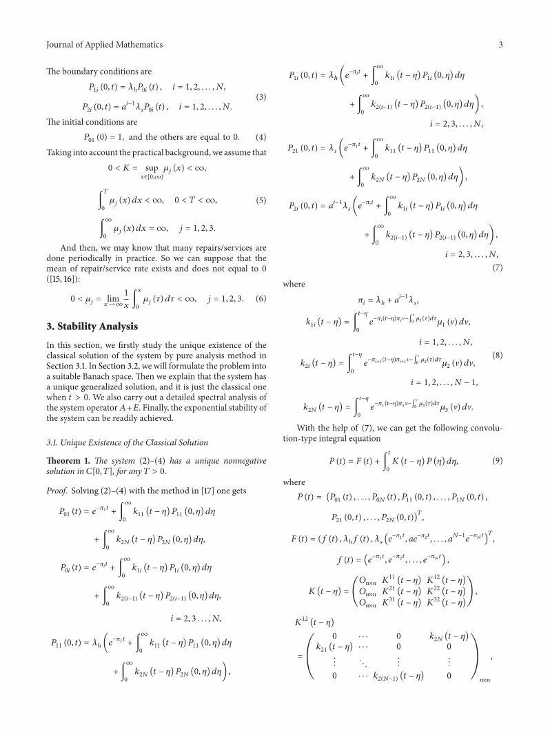2 Mathematical Model Formulation

In the reliability analysis of repair system it is usuallyassumed that the repaired units which compose system areas good as new and the failed units are repaired immediatelyHowever in reality it is usually not the case In real life it ispossible that the reliability reduces after the software failureeach time That is the condition 119865

(119899)

119878(119905) = 119865

119878(119886119899minus1

119905) = 1minus

119890minus119886119899minus1

120582119904119905 119905 ge 0 120582

119904gt 0 and the coefficient 119886 gt 1 With

the number of repair times increasing the failure rate isincreasing gradually In view of the aging and accumulativewear the repair time will become longer and longer andtend towards infinity that is the system is nonrepairableTherefore we first suppose that the software is overhauled(replaced) to be as good as new after the (119873 minus 1)th minimalrepair and studying the number of minimal repair beforeoverhaul repair is more appropriate And we will also discusshow its reliability will be affected by the number of minimalrepair and overhaul In [14] the author supposed that thesoftware cannot be repaired as good as new and utilized thegeometric process and supplementary variable technique toanalyze the system reliability However the life and repairtimes of the hardware and software are supposed to followexponential distribution In this paper under assumptionthat the life time of the hardware and software follows expo-nential distribution and repair time is subject to the generaldistribution we set up amathematicalmodel of the repairablecomputer system by the supplementary variable methodwhich is composed of the hardware and software in seriesThe hardware is repaired to be as good as new the softwareis repaired periodically and restored software life decreasesAfter a period of time an overhaul makes it as a new one

The system model is formulated specifically as follows

(i) The computer system is composed of hardware119867 andsoftware 119878 in series

(ii) The distribution function of the life time 119883119867

ofhardware119867 is 119865

119867(119905) = 1 minus 119890

minus120582ℎ119905 119905 ge 0 120582

ℎgt 0

(iii) The distribution function of the life time119883(119899)119878

of soft-ware 119878 during its 119899th period (eg the time betweenthe completion of its (119899 minus 1)th repair and that of the119899th repair) is 119865119899

119878(119905) = 119865

119878(119886119899minus1

119905) = 1 minus 119890minus119886119899minus1

120582119904119905 119905 ge 0

120582119904gt 0 119886 gt 1 119899 = 1 2 119873

(iv) Let 1198841be the repair time of hardware119867 119884

2the repair

time of software 119878 after its 119899th failure (119899 = 1 2 119873minus

1) and 1198843the repair time of software 119878 after its 119899th

failure respectively Their distribution functions are119866119895(119905) = int

119905

0119892119895(119909)119889119909 = 1minus119890

minusint119905

0

120583119895(119909)119889119909 and119864[119884

119895] = 1120583

119895

119895 = 1 2 3 where 1205833(119909) gt 120583

2(119909) for all 119909 ge 0

(v) The hardware 119867 is repaired as good as new Thesoftware 119878 is performed by a minimal repair (eg amaintenance action performed on a failed system bywhich its survival time is decreasing) during its 119899th(119899 = 1 2 119873 minus 1) period and an overhaul repair(eg a maintenance action performed on a failedsystem by which it is repaired as good as new) during

its 119873th period The above stochastic variables areindependent of each other

Let 119873(119905) be the system state at time 119905 and assume all thepossible states as below

0119894 (119894 = 1 2 119873) the system is working1119894 (119894 = 1 2 119873) the system is failed because the failure

hardware119867 is being repaired in the 119894th time2119894 (119894 = 1 2 119873) the system has in failure state because

the failure software 119878 is being repaired minimally in the119894th time (119894 = 1 2 119873 minus 1) and the software 119878 is beingoverhauled in the119873th time

Then the system state space is 119864 = 0119894 1119894 2119894 (119894 =

1 2 119873) in which the working state space is 119882 = 0119894

(119894 = 1 2 119873) and the failure state space is 119865 = 1119894 2119894

(119894 = 1 2 119873)When 119873(119905) = 119895119894 (119895 = 0 1 2 119894 = 1 2 119873) supple-

ment variable 119884119895(119905) (119895 = 1 2 3) which denotes the elapsed

repair time of hardware 119867 the elapsed minimal repairtime of software 119878 and its elapsed overhaul time at time 119905respectively then 119873(119905) 119884

119895(119905) constitutes a matrix Markov

process whose state probabilities are defined as follows

1198750119894 (

119905) = 119875 119873 (119905) = 0119894 119894 = 1 2 119873

1198751119894 (

119909 119905) = 119875 119909 lt 1198841 (

119905) le 119909 + 119889119909119873 (119905) = 1119894

119894 = 1 2 119873

1198752119894(119909 119905) = 119875 119909 lt 119884

2(119905) le 119909 + 119889119909119873 (119905) = 2119894

119894 = 1 2 119873 minus 1

1198752119873

(119909 119905) = 119875 119909 lt 1198843(119905) le 119909 + 119889119909119873 (119905) = 2119873

(1)

Then by using the method of probability analysis the systemunder consideration can be formulated as the following equa-tions

11988911987501 (

119905)

119889119905

= minus (120582ℎ+ 120582119904) 11987501 (

119905) + int

infin

0

11987511 (

119909 119905) 1205831 (119909) 119889119909

+ int

infin

0

1198752119873 (

119909 119905) 1205833 (119909) 119889119909

1198891198750119894(119905)

119889119905

= minus (120582ℎ+ 119886119894minus1

120582119904) 1198750119894(119905) + int

infin

0

1198751119894(119909 119905) 120583

1(119909) 119889119909

+ int

infin

0

1198752(119894minus1)

(119909 119905) 1205832(119909) 119889119909

119894 = 2 3 119873

1205971198751119894 (

119909 119905)

120597119909

+

1205971198751119894 (

119909 119905)

120597119905

= minus1205831 (

119909) 1198751119894 (119909 119905)

119894 = 1 2 119873

1205971198752119894(119909 119905)

120597119909

+

1205971198752119894(119909 119905)

120597119905

= minus1205832(119909) 1198752119894(119909 119905)

119894 = 1 2 119873 minus 1

1205971198752119873

(119909 119905)

120597119909

+

1205971198752119873

(119909 119905)

120597119905

= minus1205833(119909) 1198752119873

(119909 119905)

(2)



0 119905) = 120582ℎ1198750119894 (

119905) 119894 = 1 2 119873

1198752119894 (

0 119905) = 119886119894minus1

1205821199041198750119894 (

119905) 119894 = 1 2 119873

(3)




120583119895(119909) lt infin

int

119879

0


int

infin

0

120583119895 (119909) 119889119909 = infin 119895 = 1 2 3

(5)


0 lt 120583119895= lim119909rarrinfin

1

119909

int

119909

0

120583119895 (120591) 119889120591 lt infin 119895 = 1 2 3 (6)






11987501 (

119905) = 119890minus1205871119905+ int

infin

0

11989611

(119905 minus 120578) 11987511

(0 120578) 119889120578

+ int

infin

0

1198962119873

(119905 minus 120578) 1198752119873

(0 120578) 119889120578

1198750119894(119905) = 119890

minus120587119894119905+ int

infin

0

1198961119894(119905 minus 120578) 119875

1119894(0 120578) 119889120578

+ int

infin

0

1198962(119894minus1)

(119905 minus 120578) 1198752(119894minus1)

(0 120578) 119889120578

119894 = 2 3 119873

11987511

(0 119905) = 120582ℎ(119890minus1205871119905+ int

infin

0

11989611

(119905 minus 120578) 11987511

(0 120578) 119889120578

+int

infin

0

1198962119873

(119905 minus 120578) 1198752119873

(0 120578) 119889120578)

1198751119894 (

0 119905) = 120582ℎ(119890minus120587119894119905+ int

infin

0

1198961119894(119905 minus 120578) 119875

1119894(0 120578) 119889120578

+int

infin

0

1198962(119894minus1)

(119905 minus 120578) 1198752(119894minus1)

(0 120578) 119889120578)

119894 = 2 3 119873

11987521 (

0 119905) = 120582119904(119890minus1205871119905+ int

infin

0

11989611

(119905 minus 120578) 11987511

(0 120578) 119889120578

+int

infin

0

1198962119873

(119905 minus 120578) 1198752119873

(0 120578) 119889120578)

1198752119894 (

0 119905) = 119886119894minus1

120582119904(119890minus120587119894119905+ int

infin

0

1198961119894(119905 minus 120578) 119875

1119894(0 120578) 119889120578

+int

infin

0

1198962(119894minus1)

(119905 minus 120578) 1198752(119894minus1)

(0 120578) 119889120578)

119894 = 2 3 119873

(7)

where

120587119894= 120582ℎ+ 119886119894minus1

120582119904

1198961119894(119905 minus 120578) = int

119905minus120578

0

119890minus120587119894(119905minus120578)120587

119894Vminusint

V

0

1205831(120591)119889120591

1205831(V) 119889V

119894 = 1 2 119873

1198962119894(119905 minus 120578) = int

119905minus120578

0

119890minus120587119894+1(119905minus120578)120587

119894+1Vminusint

V

0

1205832(120591)119889120591

1205832(V) 119889V

119894 = 1 2 119873 minus 1

1198962119873

(119905 minus 120578) = int

119905minus120578

0

119890minus1205871(119905minus120578)120587

1Vminusint

V

0

1205833(120591)119889120591

1205833(V) 119889V

(8)


119875 (119905) = 119865 (119905) + int

119905

0

119870(119905 minus 120578) 119875 (120578) 119889120578 (9)

where119875 (119905) = (119875

01(119905) 119875

0119873(119905) 11987511

(0 119905) 1198751119873

(0 119905)

11987521 (

0 119905) 1198752119873 (0 119905))119879

119865 (119905) = (119891 (119905) 120582ℎ119891 (119905) 120582119904

(119890minus1205871119905 119886119890minus1205872119905 119886

119873minus1119890minus120587119873119905)

119879

119891 (119905) = (119890minus1205871119905 119890minus1205872119905 119890

minus120587119873119905)

119870 (119905 minus 120578) = (

119874119899times119899

11987011

(119905 minus 120578) 11987012

(119905 minus 120578)

119874119899times119899

11987021

(119905 minus 120578) 11987022

(119905 minus 120578)

119874119899times119899

11987031

(119905 minus 120578) 11987032

(119905 minus 120578)

)

11987012

(119905 minus 120578)

= (

0 sdot sdot sdot 0 1198962119873

(119905 minus 120578)

11989621


d


2(119873minus1)(119905 minus 120578) 0

)

119899times119899


11987022

(119905 minus 120578) = 120582ℎ11987012

(119905 minus 120578)

11987032

(119905 minus 120578)

= (



d



)

119899times119899

11987011

(119905 minus 120578) = diag (11989611

(119905 minus 120578) 11989611

(119905 minus 120578)

11989611

(119905 minus 120578))119899times119899

11987021

(119905 minus 120578) = diag (120582ℎ11989611

(119905 minus 120578) 120582ℎ11989611

(119905 minus 120578)

120582ℎ11989611

(119905 minus 120578))119899times119899

11987031

(119905 minus 120578) = diag (12058211990411989611

(119905 minus 120578) 11988612058211990411989611

(119905 minus 120578)

119886119873minus1

12058211990411989611

(119905 minus 120578))119899times119899

(10)




119883 = 119875 isin 119877119899times (1198711(119877+) times 1198711(119877+))

119899

| 119875

=

10038161003816100381610038161003816119875010038161003816100381610038161003816+

2

sum

119894=1

1003817100381710038171003817100381711987511989410038171003817100381710038171003817lt infin

(11)

where

119875 = (1198750 1198751(119909) 119875

2(119909))

1198750= (11987501 11987502 119875

0119873)119879

1198751(119909) = (119875

11(119909) 119875

12(119909) 119875

1119873(119909))119879

1198752(119909) = (119875

21(119909) 119875

22(119909) 119875

2119873(119909))119879

10038161003816100381610038161003816119875010038161003816100381610038161003816=

119873

sum

119894=1

10038161003816100381610038161198750119894

1003816100381610038161003816

1003816100381610038161003816100381611987511989510038161003816100381610038161003816=

119873

sum

119894=1

10038171003817100381710038171003817119875119895119894

100381710038171003817100381710038171198711(119877+) 119895 = 1 2

(12)



ℎ+ 119886120582119904) minus(120582

ℎ+

119886119873minus1

120582119904))1198750 diag(minus(119889119889119909)minus120583

1(119909) minus(119889119889119909)minus120583

1(119909))1198751(119909)


2(119909) minus(119889119889119909) minus

1205833(119909))1198752(119909))

Taking 119863(119860) = 119875 = (1198750 1198751(119909) 119875

2(119909)) isin 119883 | (119889119875

119895119894(119909)

119889119909) isin 1198711(119877+) 119895 = 1 2 119894 = 1 2 119873119875

119895119894(119909) (119895 = 1 2 119894 = 1 2


(1198750 1198751(0) 1198752(0))=(119875

0 120582ℎ1198750 120582119904(11987501 11988611987502 119886

119873minus11198750119873

)119879)

119864119875 = (

119874119899times119899

1198641

1198642

1198742119899times119899

1198742119899times119899

1198742119899times119899

)(

1198750

1198751(119909)

1198752(119909)

) 119863 (119864) = 119883

(13)

where 119874119899times119899

1198742119899times119899


= diag(1205831(119909)

1205831(119909) 120583

1(119909))119899times119899

1198642

=

(

(

(

(

(


infin

0

1205833(119909) 119889119909

0 int

infin

0

1205832(119909) 119889119909 sdot sdot sdot 0 0

d


infin

0

1205832(119909) 119889119909 0

)

)

)

)

)119899times119899

(14)


119889

119889119905

119875 (sdot 119905) = (119860 + 119864) 119875 (sdot 119905) 119905 ge 0

119875 (sdot 119905) = (1198750(119905) 1198751(sdot 119905) 119875

2(sdot 119905))

119875 (sdot 0) = 1198750= ((1 0 0)

119879

1times119899 119874119899times1

119874119899times1

)

(15)


0semigroup theory




(see [18])

int

infin

119905


119905

120583119895(120591)119889120591

119889119909 le 119871 119895 = 1 2 3 (16)


119877 119886 = 0 (see [18])10038161003816100381610038161003816100381610038161003816

int

infin

0

120583119895 (119909) 119890minusint119909

0

(119903+120583119895(120591))119889120591

119889119909

10038161003816100381610038161003816100381610038161003816

lt 1 119895 = 1 2 3 (17)






119895=

(1198921198951 1198921198952 119892


119866 That is

(119903 + 120582ℎ+ 120582119904) 11987501

minus int

infin

0

1205831(119909) 11987511

(119909) 119889119909

minus int

infin

0

1205833(119909) 1198752119873

(119909) 119889119909 = 11989201

(18)

(119903 + 120582ℎ+ 119886119895minus1

120582119904) 1198750119895

minus int

infin

0

1205831 (

119909) 1198751119895 (119909) 119889119909

minus int

infin

0

1205832(119909) 1198752(119895minus1)

(119909) 119889119909 = 1198920119895

119895 = 2 119873

(19)

119889

119889119909

1198751119895 (

119909) + (119903 + 1205831 (

119909)) 1198751119895 (119909) = 119892

1119895 (119909)

119895 = 1 2 119873

(20)

119889

119889119909

1198752119895 (

119909) + (119903 + 1205832 (

119909)) 1198752119895 (119909) = 119892

2119895 (119909)

119895 = 2 3 119873 minus 1

(21)

119889

119889119909

1198752119873 (

119909) + (119903 + 1205833 (

119909)) 1198752119873 (119909) = 119892

2119873 (119909) (22)

And we can suppose

1198751119895(0) = 120582

ℎ1198750119895 119895 = 1 2 119873

1198752119895(0) = 119886

119895minus11205821199041198750119895 119895 = 1 2 119873

(23)


1198751119895 (

119909) = 1198751119895 (

0) 119890minusint119909

0

[119903+1205831(120578)]119889120578

+ int

119909

0


120591

[119903+1205831(120578)]119889120578

1198921119895 (

120591) 119889120591

119895 = 1 2 119873

1198752119895 (

119909) = 1198752119895 (

0) 119890minusint119909

0

[119903+1205832(120578)]119889120578

+ int

119909

0


120591

[119903+1205832(120578)]119889120578

1198922119895 (

120591) 119889120591

119895 = 1 2 119873 minus 1

1198752119873

(119909)=1198752119873

(0) 119890minusint119909

0

[119903+1205833(120578)]119889120578

+int

119909

0


120591

[119903+1205833(120578)]119889120578

1198922119873

(120591) 119889120591

(24)


1[0infin) 119895 = 1 2 119894 = 1 2 119873


1[0infin) 119895 = 1 2





(

(

(

(

(

119903 + 1198871


1205821199041198823

minus1205821199041198822

119903 + 1198872

sdot sdot sdot 0 0

0 minus1198861205821199041198822

d 0 0

d


0


1205821199041198822

119903 + 119887119873

)

)

)

)

)

times

(

(

(

(

11987501

11987502

11987503

1198750(119873minus1)

1198750119873

)

)

)

)

=(

(

(

0

0

0

0

0

)

)

)

(25)

where

119887119895= 120582ℎ(1 minus 119882

1) + 119886119895minus1

120582119904

(119895 = 1 2 119873)

119882119895= int

infin

0

120583119895(119909) 119890minusint119909

0

[119903+120583119895(120591)]119889120591

119889119909 119895 = 1 2 3

(26)

It is clear that10038161003816100381610038161003816119903 + 119887119895

10038161003816100381610038161003816=

10038161003816100381610038161003816119903 + 120582ℎ(1 minus 119882

1) + 119886119895minus1

120582119904

10038161003816100381610038161003816gt

10038161003816100381610038161003816119903 + 119886119895minus1

120582119904

10038161003816100381610038161003816

gt

10038161003816100381610038161003816119886119895minus1

120582119904

10038161003816100381610038161003816gt

10038161003816100381610038161003816minus119886119895minus1

1205821199041198822

10038161003816100381610038161003816 119895 = 1 2 119873 minus 1

1003816100381610038161003816119903 + 119887119873

1003816100381610038161003816=

10038161003816100381610038161003816119903 + 120582ℎ(1 minus 119882

1) + 119886119873minus1

120582119904

10038161003816100381610038161003816gt

10038161003816100381610038161003816119903 + 119886119873minus1

120582119904

10038161003816100381610038161003816

gt

10038161003816100381610038161003816119886119873minus1

120582119904

10038161003816100381610038161003816gt

10038161003816100381610038161003816minus119886119873minus1

1205821199041198823

10038161003816100381610038161003816gt 0

(27)












1198750119895

= 119886119873minus119895

1198750119873

(119895 = 1 2 119873)

1198751119895(119909) = 119886

119873minus119895120582ℎ1198750119873


0

1205831(120578)119889120578

(119895 = 1 2 119873)

1198752119895(119909) = 119886

119873minus1198951205821199041198750119873


0

1205832(120578)119889120578

(119895 = 1 2 119873 minus 1)

1198752119873

(119909) = 119886119873minus1

1205821199041198750119873


0

1205833(120578)119889120578

(28)

where 1198750119873



taking 1198750119873


119875lowast= ((119875

lowast

01 119875

lowast

0119873)119879 (119875lowast

11(119909) 119875

lowast

1119873(119909))119879

(119875lowast

21(119909) 119875

lowast

2119873(119909))119879)

(29)


0119894and 119875

lowast

119895119894(119909) respectively

signify 1198750119894and 119875

119895119894(119909) showed in (28) 119895 = 1 2 119894 = 1 2 119873



Taking vector 119876 = (1198680

119899times1 1198681

119899times1 1198682

119899times1) here 119868

119895= (1 1

1)119879 119895 = 0 1 2 Then 119876 isin 119883







⟨119875lowast 119876⟩ = ⟨(119860 + 119864)119880119876⟩ = ⟨119880 (119860 + 119864)

lowast119876⟩ = 0

(30)

However

⟨119875lowast 119876⟩ =

119873

sum

119894=1

1198750119894+

2

sum

119895=1

119873

sum

119894=1

int

infin

0

119875119895119894(119909) 119889119909 gt 0 (31)




0semigroups 119879(119905)


0semigroup 119879(119905)






0 = 119875

0 = 1 for all










0 for all


119875 (sdot 119905) = 119879 (119905) 1198750= ⟨1198750 119876⟩ 119875

lowast+ 119877 (119905) 119875

0= 119875lowast+ 119877 (119905) 119875

0

(33)



lim119905rarrinfin

119875 (sdot 119905) = ⟨1198750 119876⟩ 119875









0119894(119905) rarr 119875

0119894gt 0






(120582ℎ+ 120582119904) 11987501

= int

infin

0

11987511

(119909) 1205831(119909) 119889119909 + int

infin

0

1198752119873

(119909) 1205833(119909) 119889119909

(120582ℎ+ 119886119894minus1

120582119904) 1198750119894= int

infin

0

1198751119894 (

119909) 1205831 (119909) 119889119909

+ int

infin

0

1198752(119894minus1)

(119909) 1205832(119909) 119889119909

119894 = 2 3 119873

(

119889

119889119909

+ 1205831 (

119909))1198751119894 (

119909) = 0 119894 = 1 2 119873

(

119889

119889119909

+ +1205832(119909))119875

2119894(119909) = 0 119894 = 1 2 119873 minus 1

(

119889

119889119909

+ 1205833(119909))119875

2119873(119909) = 0

(35)


1198751119894(0) = 120582

ℎ1198750119894 119894 = 1 2 119873

1198752119894(0) = 119886

119894minus11205821199041198750119894 119894 = 1 2 119873

(36)


+infin

01198751119894(119909)119889119909

1198752119894

= int

+infin



119873

sum

119894=1

(1198750119894+ 1198751119894+ 1198752119894) = 1 (37)


=

sum119873

119894=1(1198751119894+ 1198752119894) and 119865

119891= sum119873

119894=1(120582ℎ+ 119886119894minus1

120582119904)1198750119894



119860V119873 =

sum119873

119894=1119886119894minus1

sum119873

119894=1119886119894minus1

(1 + 120582ℎ1198641) + 119886119873minus1

120582119904[(119873 minus 1) 119864

2+ 1198643]

(38)

where 119864119894= int

infin

0119890minusint119909

0

120583119894(119904)119889119904

119889119909 (119894 = 1 2 3)

Proof Let

119872 =

2

sum

119895=0

119873

sum

119894=1

119875lowast

119895119894≜

119873

sum

119894=1

119875lowast

0119894+

119873

sum

119894=1

int

infin

0

119875lowast

1119894(119909) 119889119909 +

119873

sum

119894=1

int

infin

0

119875lowast

2119894(119909) 119889119909

=

119873

sum

119894=1

119886119894minus1

(1 + 120582ℎ1198641) + 119886119873minus1

120582119904[(119873 minus 1) 119864

2+ 1198643]119875lowast

0119873

(39)




119860V119873 =

sum119873

119894=1119875lowast

0119894

sum119873

119894=1(119875lowast

0119894+ 119875lowast

1119894(119909) + 119875

lowast

2119894(119909))

(40)

=

sum119873

119894=1119886119894minus1

sum119873

119894=1119886119894minus1

(1 + 120582ℎ1198641) + 119886119873minus1

120582119904[(119873 minus 1) 1198642

+ 1198643]

(41)

where 119864119894= int

infin

0119890minusint119909

0

120583119894(119904)119889119904

119889119909 (119894 = 1 2 3)



119882119891119873

=

120582ℎsum119873

119894=1119886119894minus1

+ 120582119904119873119886119873minus1

sum119873

119894=1119886119894minus1

(1 + 120582ℎ1198641) + 119886119873minus1

120582119904[(119873 minus 1) 119864

2+ 1198643]

(42)

where 119864119894= int

infin

0119890minusint119909

0

120583119894(119904)119889119904

119889119909 (119894 = 1 2 3)






5 Conclusion



Acknowledgments


References





































Volume 2014




Journal of











Journal of


Function Spaces






Algebra











0 119905) = 120582ℎ1198750119894 (

119905) 119894 = 1 2 119873

1198752119894 (

0 119905) = 119886119894minus1

1205821199041198750119894 (

119905) 119894 = 1 2 119873

(3)




120583119895(119909) lt infin

int

119879

0


int

infin

0

120583119895 (119909) 119889119909 = infin 119895 = 1 2 3

(5)


0 lt 120583119895= lim119909rarrinfin

1

119909

int

119909

0

120583119895 (120591) 119889120591 lt infin 119895 = 1 2 3 (6)






11987501 (

119905) = 119890minus1205871119905+ int

infin

0

11989611

(119905 minus 120578) 11987511

(0 120578) 119889120578

+ int

infin

0

1198962119873

(119905 minus 120578) 1198752119873

(0 120578) 119889120578

1198750119894(119905) = 119890

minus120587119894119905+ int

infin

0

1198961119894(119905 minus 120578) 119875

1119894(0 120578) 119889120578

+ int

infin

0

1198962(119894minus1)

(119905 minus 120578) 1198752(119894minus1)

(0 120578) 119889120578

119894 = 2 3 119873

11987511

(0 119905) = 120582ℎ(119890minus1205871119905+ int

infin

0

11989611

(119905 minus 120578) 11987511

(0 120578) 119889120578

+int

infin

0

1198962119873

(119905 minus 120578) 1198752119873

(0 120578) 119889120578)

1198751119894 (

0 119905) = 120582ℎ(119890minus120587119894119905+ int

infin

0

1198961119894(119905 minus 120578) 119875

1119894(0 120578) 119889120578

+int

infin

0

1198962(119894minus1)

(119905 minus 120578) 1198752(119894minus1)

(0 120578) 119889120578)

119894 = 2 3 119873

11987521 (

0 119905) = 120582119904(119890minus1205871119905+ int

infin

0

11989611

(119905 minus 120578) 11987511

(0 120578) 119889120578

+int

infin

0

1198962119873

(119905 minus 120578) 1198752119873

(0 120578) 119889120578)

1198752119894 (

0 119905) = 119886119894minus1

120582119904(119890minus120587119894119905+ int

infin

0

1198961119894(119905 minus 120578) 119875

1119894(0 120578) 119889120578

+int

infin

0

1198962(119894minus1)

(119905 minus 120578) 1198752(119894minus1)

(0 120578) 119889120578)

119894 = 2 3 119873

(7)

where

120587119894= 120582ℎ+ 119886119894minus1

120582119904

1198961119894(119905 minus 120578) = int

119905minus120578

0

119890minus120587119894(119905minus120578)120587

119894Vminusint

V

0

1205831(120591)119889120591

1205831(V) 119889V

119894 = 1 2 119873

1198962119894(119905 minus 120578) = int

119905minus120578

0

119890minus120587119894+1(119905minus120578)120587

119894+1Vminusint

V

0

1205832(120591)119889120591

1205832(V) 119889V

119894 = 1 2 119873 minus 1

1198962119873

(119905 minus 120578) = int

119905minus120578

0

119890minus1205871(119905minus120578)120587

1Vminusint

V

0

1205833(120591)119889120591

1205833(V) 119889V

(8)


119875 (119905) = 119865 (119905) + int

119905

0

119870(119905 minus 120578) 119875 (120578) 119889120578 (9)

where119875 (119905) = (119875

01(119905) 119875

0119873(119905) 11987511

(0 119905) 1198751119873

(0 119905)

11987521 (

0 119905) 1198752119873 (0 119905))119879

119865 (119905) = (119891 (119905) 120582ℎ119891 (119905) 120582119904

(119890minus1205871119905 119886119890minus1205872119905 119886

119873minus1119890minus120587119873119905)

119879

119891 (119905) = (119890minus1205871119905 119890minus1205872119905 119890

minus120587119873119905)

119870 (119905 minus 120578) = (

119874119899times119899

11987011

(119905 minus 120578) 11987012

(119905 minus 120578)

119874119899times119899

11987021

(119905 minus 120578) 11987022

(119905 minus 120578)

119874119899times119899

11987031

(119905 minus 120578) 11987032

(119905 minus 120578)

)

11987012

(119905 minus 120578)

= (

0 sdot sdot sdot 0 1198962119873

(119905 minus 120578)

11989621


d


2(119873minus1)(119905 minus 120578) 0

)

119899times119899


11987022

(119905 minus 120578) = 120582ℎ11987012

(119905 minus 120578)

11987032

(119905 minus 120578)

= (



d



)

119899times119899

11987011

(119905 minus 120578) = diag (11989611

(119905 minus 120578) 11989611

(119905 minus 120578)

11989611

(119905 minus 120578))119899times119899

11987021

(119905 minus 120578) = diag (120582ℎ11989611

(119905 minus 120578) 120582ℎ11989611

(119905 minus 120578)

120582ℎ11989611

(119905 minus 120578))119899times119899

11987031

(119905 minus 120578) = diag (12058211990411989611

(119905 minus 120578) 11988612058211990411989611

(119905 minus 120578)

119886119873minus1

12058211990411989611

(119905 minus 120578))119899times119899

(10)




119883 = 119875 isin 119877119899times (1198711(119877+) times 1198711(119877+))

119899

| 119875

=

10038161003816100381610038161003816119875010038161003816100381610038161003816+

2

sum

119894=1

1003817100381710038171003817100381711987511989410038171003817100381710038171003817lt infin

(11)

where

119875 = (1198750 1198751(119909) 119875

2(119909))

1198750= (11987501 11987502 119875

0119873)119879

1198751(119909) = (119875

11(119909) 119875

12(119909) 119875

1119873(119909))119879

1198752(119909) = (119875

21(119909) 119875

22(119909) 119875

2119873(119909))119879

10038161003816100381610038161003816119875010038161003816100381610038161003816=

119873

sum

119894=1

10038161003816100381610038161198750119894

1003816100381610038161003816

1003816100381610038161003816100381611987511989510038161003816100381610038161003816=

119873

sum

119894=1

10038171003817100381710038171003817119875119895119894

100381710038171003817100381710038171198711(119877+) 119895 = 1 2

(12)



ℎ+ 119886120582119904) minus(120582

ℎ+

119886119873minus1

120582119904))1198750 diag(minus(119889119889119909)minus120583

1(119909) minus(119889119889119909)minus120583

1(119909))1198751(119909)


2(119909) minus(119889119889119909) minus

1205833(119909))1198752(119909))

Taking 119863(119860) = 119875 = (1198750 1198751(119909) 119875

2(119909)) isin 119883 | (119889119875

119895119894(119909)

119889119909) isin 1198711(119877+) 119895 = 1 2 119894 = 1 2 119873119875

119895119894(119909) (119895 = 1 2 119894 = 1 2


(1198750 1198751(0) 1198752(0))=(119875

0 120582ℎ1198750 120582119904(11987501 11988611987502 119886

119873minus11198750119873

)119879)

119864119875 = (

119874119899times119899

1198641

1198642

1198742119899times119899

1198742119899times119899

1198742119899times119899

)(

1198750

1198751(119909)

1198752(119909)

) 119863 (119864) = 119883

(13)

where 119874119899times119899

1198742119899times119899


= diag(1205831(119909)

1205831(119909) 120583

1(119909))119899times119899

1198642

=

(

(

(

(

(


infin

0

1205833(119909) 119889119909

0 int

infin

0

1205832(119909) 119889119909 sdot sdot sdot 0 0

d


infin

0

1205832(119909) 119889119909 0

)

)

)

)

)119899times119899

(14)


119889

119889119905

119875 (sdot 119905) = (119860 + 119864) 119875 (sdot 119905) 119905 ge 0

119875 (sdot 119905) = (1198750(119905) 1198751(sdot 119905) 119875

2(sdot 119905))

119875 (sdot 0) = 1198750= ((1 0 0)

119879

1times119899 119874119899times1

119874119899times1

)

(15)


0semigroup theory




(see [18])

int

infin

119905


119905

120583119895(120591)119889120591

119889119909 le 119871 119895 = 1 2 3 (16)


119877 119886 = 0 (see [18])10038161003816100381610038161003816100381610038161003816

int

infin

0

120583119895 (119909) 119890minusint119909

0

(119903+120583119895(120591))119889120591

119889119909

10038161003816100381610038161003816100381610038161003816

lt 1 119895 = 1 2 3 (17)






119895=

(1198921198951 1198921198952 119892


119866 That is

(119903 + 120582ℎ+ 120582119904) 11987501

minus int

infin

0

1205831(119909) 11987511

(119909) 119889119909

minus int

infin

0

1205833(119909) 1198752119873

(119909) 119889119909 = 11989201

(18)

(119903 + 120582ℎ+ 119886119895minus1

120582119904) 1198750119895

minus int

infin

0

1205831 (

119909) 1198751119895 (119909) 119889119909

minus int

infin

0

1205832(119909) 1198752(119895minus1)

(119909) 119889119909 = 1198920119895

119895 = 2 119873

(19)

119889

119889119909

1198751119895 (

119909) + (119903 + 1205831 (

119909)) 1198751119895 (119909) = 119892

1119895 (119909)

119895 = 1 2 119873

(20)

119889

119889119909

1198752119895 (

119909) + (119903 + 1205832 (

119909)) 1198752119895 (119909) = 119892

2119895 (119909)

119895 = 2 3 119873 minus 1

(21)

119889

119889119909

1198752119873 (

119909) + (119903 + 1205833 (

119909)) 1198752119873 (119909) = 119892

2119873 (119909) (22)

And we can suppose

1198751119895(0) = 120582

ℎ1198750119895 119895 = 1 2 119873

1198752119895(0) = 119886

119895minus11205821199041198750119895 119895 = 1 2 119873

(23)


1198751119895 (

119909) = 1198751119895 (

0) 119890minusint119909

0

[119903+1205831(120578)]119889120578

+ int

119909

0


120591

[119903+1205831(120578)]119889120578

1198921119895 (

120591) 119889120591

119895 = 1 2 119873

1198752119895 (

119909) = 1198752119895 (

0) 119890minusint119909

0

[119903+1205832(120578)]119889120578

+ int

119909

0


120591

[119903+1205832(120578)]119889120578

1198922119895 (

120591) 119889120591

119895 = 1 2 119873 minus 1

1198752119873

(119909)=1198752119873

(0) 119890minusint119909

0

[119903+1205833(120578)]119889120578

+int

119909

0


120591

[119903+1205833(120578)]119889120578

1198922119873

(120591) 119889120591

(24)


1[0infin) 119895 = 1 2 119894 = 1 2 119873


1[0infin) 119895 = 1 2





(

(

(

(

(

119903 + 1198871


1205821199041198823

minus1205821199041198822

119903 + 1198872

sdot sdot sdot 0 0

0 minus1198861205821199041198822

d 0 0

d


0


1205821199041198822

119903 + 119887119873

)

)

)

)

)

times

(

(

(

(

11987501

11987502

11987503

1198750(119873minus1)

1198750119873

)

)

)

)

=(

(

(

0

0

0

0

0

)

)

)

(25)

where

119887119895= 120582ℎ(1 minus 119882

1) + 119886119895minus1

120582119904

(119895 = 1 2 119873)

119882119895= int

infin

0

120583119895(119909) 119890minusint119909

0

[119903+120583119895(120591)]119889120591

119889119909 119895 = 1 2 3

(26)

It is clear that10038161003816100381610038161003816119903 + 119887119895

10038161003816100381610038161003816=

10038161003816100381610038161003816119903 + 120582ℎ(1 minus 119882

1) + 119886119895minus1

120582119904

10038161003816100381610038161003816gt

10038161003816100381610038161003816119903 + 119886119895minus1

120582119904

10038161003816100381610038161003816

gt

10038161003816100381610038161003816119886119895minus1

120582119904

10038161003816100381610038161003816gt

10038161003816100381610038161003816minus119886119895minus1

1205821199041198822

10038161003816100381610038161003816 119895 = 1 2 119873 minus 1

1003816100381610038161003816119903 + 119887119873

1003816100381610038161003816=

10038161003816100381610038161003816119903 + 120582ℎ(1 minus 119882

1) + 119886119873minus1

120582119904

10038161003816100381610038161003816gt

10038161003816100381610038161003816119903 + 119886119873minus1

120582119904

10038161003816100381610038161003816

gt

10038161003816100381610038161003816119886119873minus1

120582119904

10038161003816100381610038161003816gt

10038161003816100381610038161003816minus119886119873minus1

1205821199041198823

10038161003816100381610038161003816gt 0

(27)












1198750119895

= 119886119873minus119895

1198750119873

(119895 = 1 2 119873)

1198751119895(119909) = 119886

119873minus119895120582ℎ1198750119873


0

1205831(120578)119889120578

(119895 = 1 2 119873)

1198752119895(119909) = 119886

119873minus1198951205821199041198750119873


0

1205832(120578)119889120578

(119895 = 1 2 119873 minus 1)

1198752119873

(119909) = 119886119873minus1

1205821199041198750119873


0

1205833(120578)119889120578

(28)

where 1198750119873



taking 1198750119873


119875lowast= ((119875

lowast

01 119875

lowast

0119873)119879 (119875lowast

11(119909) 119875

lowast

1119873(119909))119879

(119875lowast

21(119909) 119875

lowast

2119873(119909))119879)

(29)


0119894and 119875

lowast

119895119894(119909) respectively

signify 1198750119894and 119875

119895119894(119909) showed in (28) 119895 = 1 2 119894 = 1 2 119873



Taking vector 119876 = (1198680

119899times1 1198681

119899times1 1198682

119899times1) here 119868

119895= (1 1

1)119879 119895 = 0 1 2 Then 119876 isin 119883







⟨119875lowast 119876⟩ = ⟨(119860 + 119864)119880119876⟩ = ⟨119880 (119860 + 119864)

lowast119876⟩ = 0

(30)

However

⟨119875lowast 119876⟩ =

119873

sum

119894=1

1198750119894+

2

sum

119895=1

119873

sum

119894=1

int

infin

0

119875119895119894(119909) 119889119909 gt 0 (31)




0semigroups 119879(119905)


0semigroup 119879(119905)






0 = 119875

0 = 1 for all










0 for all


119875 (sdot 119905) = 119879 (119905) 1198750= ⟨1198750 119876⟩ 119875

lowast+ 119877 (119905) 119875

0= 119875lowast+ 119877 (119905) 119875

0

(33)



lim119905rarrinfin

119875 (sdot 119905) = ⟨1198750 119876⟩ 119875









0119894(119905) rarr 119875

0119894gt 0






(120582ℎ+ 120582119904) 11987501

= int

infin

0

11987511

(119909) 1205831(119909) 119889119909 + int

infin

0

1198752119873

(119909) 1205833(119909) 119889119909

(120582ℎ+ 119886119894minus1

120582119904) 1198750119894= int

infin

0

1198751119894 (

119909) 1205831 (119909) 119889119909

+ int

infin

0

1198752(119894minus1)

(119909) 1205832(119909) 119889119909

119894 = 2 3 119873

(

119889

119889119909

+ 1205831 (

119909))1198751119894 (

119909) = 0 119894 = 1 2 119873

(

119889

119889119909

+ +1205832(119909))119875

2119894(119909) = 0 119894 = 1 2 119873 minus 1

(

119889

119889119909

+ 1205833(119909))119875

2119873(119909) = 0

(35)


1198751119894(0) = 120582

ℎ1198750119894 119894 = 1 2 119873

1198752119894(0) = 119886

119894minus11205821199041198750119894 119894 = 1 2 119873

(36)


+infin

01198751119894(119909)119889119909

1198752119894

= int

+infin



119873

sum

119894=1

(1198750119894+ 1198751119894+ 1198752119894) = 1 (37)


=

sum119873

119894=1(1198751119894+ 1198752119894) and 119865

119891= sum119873

119894=1(120582ℎ+ 119886119894minus1

120582119904)1198750119894



119860V119873 =

sum119873

119894=1119886119894minus1

sum119873

119894=1119886119894minus1

(1 + 120582ℎ1198641) + 119886119873minus1

120582119904[(119873 minus 1) 119864

2+ 1198643]

(38)

where 119864119894= int

infin

0119890minusint119909

0

120583119894(119904)119889119904

119889119909 (119894 = 1 2 3)

Proof Let

119872 =

2

sum

119895=0

119873

sum

119894=1

119875lowast

119895119894≜

119873

sum

119894=1

119875lowast

0119894+

119873

sum

119894=1

int

infin

0

119875lowast

1119894(119909) 119889119909 +

119873

sum

119894=1

int

infin

0

119875lowast

2119894(119909) 119889119909

=

119873

sum

119894=1

119886119894minus1

(1 + 120582ℎ1198641) + 119886119873minus1

120582119904[(119873 minus 1) 119864

2+ 1198643]119875lowast

0119873

(39)




119860V119873 =

sum119873

119894=1119875lowast

0119894

sum119873

119894=1(119875lowast

0119894+ 119875lowast

1119894(119909) + 119875

lowast

2119894(119909))

(40)

=

sum119873

119894=1119886119894minus1

sum119873

119894=1119886119894minus1

(1 + 120582ℎ1198641) + 119886119873minus1

120582119904[(119873 minus 1) 1198642

+ 1198643]

(41)

where 119864119894= int

infin

0119890minusint119909

0

120583119894(119904)119889119904

119889119909 (119894 = 1 2 3)



119882119891119873

=

120582ℎsum119873

119894=1119886119894minus1

+ 120582119904119873119886119873minus1

sum119873

119894=1119886119894minus1

(1 + 120582ℎ1198641) + 119886119873minus1

120582119904[(119873 minus 1) 119864

2+ 1198643]

(42)

where 119864119894= int

infin

0119890minusint119909

0

120583119894(119904)119889119904

119889119909 (119894 = 1 2 3)






5 Conclusion



Acknowledgments


References





































Volume 2014




Journal of











Journal of


Function Spaces






Algebra










11987022

(119905 minus 120578) = 120582ℎ11987012

(119905 minus 120578)

11987032

(119905 minus 120578)

= (



d



)

119899times119899

11987011

(119905 minus 120578) = diag (11989611

(119905 minus 120578) 11989611

(119905 minus 120578)

11989611

(119905 minus 120578))119899times119899

11987021

(119905 minus 120578) = diag (120582ℎ11989611

(119905 minus 120578) 120582ℎ11989611

(119905 minus 120578)

120582ℎ11989611

(119905 minus 120578))119899times119899

11987031

(119905 minus 120578) = diag (12058211990411989611

(119905 minus 120578) 11988612058211990411989611

(119905 minus 120578)

119886119873minus1

12058211990411989611

(119905 minus 120578))119899times119899

(10)




119883 = 119875 isin 119877119899times (1198711(119877+) times 1198711(119877+))

119899

| 119875

=

10038161003816100381610038161003816119875010038161003816100381610038161003816+

2

sum

119894=1

1003817100381710038171003817100381711987511989410038171003817100381710038171003817lt infin

(11)

where

119875 = (1198750 1198751(119909) 119875

2(119909))

1198750= (11987501 11987502 119875

0119873)119879

1198751(119909) = (119875

11(119909) 119875

12(119909) 119875

1119873(119909))119879

1198752(119909) = (119875

21(119909) 119875

22(119909) 119875

2119873(119909))119879

10038161003816100381610038161003816119875010038161003816100381610038161003816=

119873

sum

119894=1

10038161003816100381610038161198750119894

1003816100381610038161003816

1003816100381610038161003816100381611987511989510038161003816100381610038161003816=

119873

sum

119894=1

10038171003817100381710038171003817119875119895119894

100381710038171003817100381710038171198711(119877+) 119895 = 1 2

(12)



ℎ+ 119886120582119904) minus(120582

ℎ+

119886119873minus1

120582119904))1198750 diag(minus(119889119889119909)minus120583

1(119909) minus(119889119889119909)minus120583

1(119909))1198751(119909)


2(119909) minus(119889119889119909) minus

1205833(119909))1198752(119909))

Taking 119863(119860) = 119875 = (1198750 1198751(119909) 119875

2(119909)) isin 119883 | (119889119875

119895119894(119909)

119889119909) isin 1198711(119877+) 119895 = 1 2 119894 = 1 2 119873119875

119895119894(119909) (119895 = 1 2 119894 = 1 2


(1198750 1198751(0) 1198752(0))=(119875

0 120582ℎ1198750 120582119904(11987501 11988611987502 119886

119873minus11198750119873

)119879)

119864119875 = (

119874119899times119899

1198641

1198642

1198742119899times119899

1198742119899times119899

1198742119899times119899

)(

1198750

1198751(119909)

1198752(119909)

) 119863 (119864) = 119883

(13)

where 119874119899times119899

1198742119899times119899


= diag(1205831(119909)

1205831(119909) 120583

1(119909))119899times119899

1198642

=

(

(

(

(

(


infin

0

1205833(119909) 119889119909

0 int

infin

0

1205832(119909) 119889119909 sdot sdot sdot 0 0

d


infin

0

1205832(119909) 119889119909 0

)

)

)

)

)119899times119899

(14)


119889

119889119905

119875 (sdot 119905) = (119860 + 119864) 119875 (sdot 119905) 119905 ge 0

119875 (sdot 119905) = (1198750(119905) 1198751(sdot 119905) 119875

2(sdot 119905))

119875 (sdot 0) = 1198750= ((1 0 0)

119879

1times119899 119874119899times1

119874119899times1

)

(15)


0semigroup theory




(see [18])

int

infin

119905


119905

120583119895(120591)119889120591

119889119909 le 119871 119895 = 1 2 3 (16)


119877 119886 = 0 (see [18])10038161003816100381610038161003816100381610038161003816

int

infin

0

120583119895 (119909) 119890minusint119909

0

(119903+120583119895(120591))119889120591

119889119909

10038161003816100381610038161003816100381610038161003816

lt 1 119895 = 1 2 3 (17)






119895=

(1198921198951 1198921198952 119892


119866 That is

(119903 + 120582ℎ+ 120582119904) 11987501

minus int

infin

0

1205831(119909) 11987511

(119909) 119889119909

minus int

infin

0

1205833(119909) 1198752119873

(119909) 119889119909 = 11989201

(18)

(119903 + 120582ℎ+ 119886119895minus1

120582119904) 1198750119895

minus int

infin

0

1205831 (

119909) 1198751119895 (119909) 119889119909

minus int

infin

0

1205832(119909) 1198752(119895minus1)

(119909) 119889119909 = 1198920119895

119895 = 2 119873

(19)

119889

119889119909

1198751119895 (

119909) + (119903 + 1205831 (

119909)) 1198751119895 (119909) = 119892

1119895 (119909)

119895 = 1 2 119873

(20)

119889

119889119909

1198752119895 (

119909) + (119903 + 1205832 (

119909)) 1198752119895 (119909) = 119892

2119895 (119909)

119895 = 2 3 119873 minus 1

(21)

119889

119889119909

1198752119873 (

119909) + (119903 + 1205833 (

119909)) 1198752119873 (119909) = 119892

2119873 (119909) (22)

And we can suppose

1198751119895(0) = 120582

ℎ1198750119895 119895 = 1 2 119873

1198752119895(0) = 119886

119895minus11205821199041198750119895 119895 = 1 2 119873

(23)


1198751119895 (

119909) = 1198751119895 (

0) 119890minusint119909

0

[119903+1205831(120578)]119889120578

+ int

119909

0


120591

[119903+1205831(120578)]119889120578

1198921119895 (

120591) 119889120591

119895 = 1 2 119873

1198752119895 (

119909) = 1198752119895 (

0) 119890minusint119909

0

[119903+1205832(120578)]119889120578

+ int

119909

0


120591

[119903+1205832(120578)]119889120578

1198922119895 (

120591) 119889120591

119895 = 1 2 119873 minus 1

1198752119873

(119909)=1198752119873

(0) 119890minusint119909

0

[119903+1205833(120578)]119889120578

+int

119909

0


120591

[119903+1205833(120578)]119889120578

1198922119873

(120591) 119889120591

(24)


1[0infin) 119895 = 1 2 119894 = 1 2 119873


1[0infin) 119895 = 1 2





(

(

(

(

(

119903 + 1198871


1205821199041198823

minus1205821199041198822

119903 + 1198872

sdot sdot sdot 0 0

0 minus1198861205821199041198822

d 0 0

d


0


1205821199041198822

119903 + 119887119873

)

)

)

)

)

times

(

(

(

(

11987501

11987502

11987503

1198750(119873minus1)

1198750119873

)

)

)

)

=(

(

(

0

0

0

0

0

)

)

)

(25)

where

119887119895= 120582ℎ(1 minus 119882

1) + 119886119895minus1

120582119904

(119895 = 1 2 119873)

119882119895= int

infin

0

120583119895(119909) 119890minusint119909

0

[119903+120583119895(120591)]119889120591

119889119909 119895 = 1 2 3

(26)

It is clear that10038161003816100381610038161003816119903 + 119887119895

10038161003816100381610038161003816=

10038161003816100381610038161003816119903 + 120582ℎ(1 minus 119882

1) + 119886119895minus1

120582119904

10038161003816100381610038161003816gt

10038161003816100381610038161003816119903 + 119886119895minus1

120582119904

10038161003816100381610038161003816

gt

10038161003816100381610038161003816119886119895minus1

120582119904

10038161003816100381610038161003816gt

10038161003816100381610038161003816minus119886119895minus1

1205821199041198822

10038161003816100381610038161003816 119895 = 1 2 119873 minus 1

1003816100381610038161003816119903 + 119887119873

1003816100381610038161003816=

10038161003816100381610038161003816119903 + 120582ℎ(1 minus 119882

1) + 119886119873minus1

120582119904

10038161003816100381610038161003816gt

10038161003816100381610038161003816119903 + 119886119873minus1

120582119904

10038161003816100381610038161003816

gt

10038161003816100381610038161003816119886119873minus1

120582119904

10038161003816100381610038161003816gt

10038161003816100381610038161003816minus119886119873minus1

1205821199041198823

10038161003816100381610038161003816gt 0

(27)












1198750119895

= 119886119873minus119895

1198750119873

(119895 = 1 2 119873)

1198751119895(119909) = 119886

119873minus119895120582ℎ1198750119873


0

1205831(120578)119889120578

(119895 = 1 2 119873)

1198752119895(119909) = 119886

119873minus1198951205821199041198750119873


0

1205832(120578)119889120578

(119895 = 1 2 119873 minus 1)

1198752119873

(119909) = 119886119873minus1

1205821199041198750119873


0

1205833(120578)119889120578

(28)

where 1198750119873



taking 1198750119873


119875lowast= ((119875

lowast

01 119875

lowast

0119873)119879 (119875lowast

11(119909) 119875

lowast

1119873(119909))119879

(119875lowast

21(119909) 119875

lowast

2119873(119909))119879)

(29)


0119894and 119875

lowast

119895119894(119909) respectively

signify 1198750119894and 119875

119895119894(119909) showed in (28) 119895 = 1 2 119894 = 1 2 119873



Taking vector 119876 = (1198680

119899times1 1198681

119899times1 1198682

119899times1) here 119868

119895= (1 1

1)119879 119895 = 0 1 2 Then 119876 isin 119883







⟨119875lowast 119876⟩ = ⟨(119860 + 119864)119880119876⟩ = ⟨119880 (119860 + 119864)

lowast119876⟩ = 0

(30)

However

⟨119875lowast 119876⟩ =

119873

sum

119894=1

1198750119894+

2

sum

119895=1

119873

sum

119894=1

int

infin

0

119875119895119894(119909) 119889119909 gt 0 (31)




0semigroups 119879(119905)


0semigroup 119879(119905)






0 = 119875

0 = 1 for all










0 for all


119875 (sdot 119905) = 119879 (119905) 1198750= ⟨1198750 119876⟩ 119875

lowast+ 119877 (119905) 119875

0= 119875lowast+ 119877 (119905) 119875

0

(33)



lim119905rarrinfin

119875 (sdot 119905) = ⟨1198750 119876⟩ 119875









0119894(119905) rarr 119875

0119894gt 0






(120582ℎ+ 120582119904) 11987501

= int

infin

0

11987511

(119909) 1205831(119909) 119889119909 + int

infin

0

1198752119873

(119909) 1205833(119909) 119889119909

(120582ℎ+ 119886119894minus1

120582119904) 1198750119894= int

infin

0

1198751119894 (

119909) 1205831 (119909) 119889119909

+ int

infin

0

1198752(119894minus1)

(119909) 1205832(119909) 119889119909

119894 = 2 3 119873

(

119889

119889119909

+ 1205831 (

119909))1198751119894 (

119909) = 0 119894 = 1 2 119873

(

119889

119889119909

+ +1205832(119909))119875

2119894(119909) = 0 119894 = 1 2 119873 minus 1

(

119889

119889119909

+ 1205833(119909))119875

2119873(119909) = 0

(35)


1198751119894(0) = 120582

ℎ1198750119894 119894 = 1 2 119873

1198752119894(0) = 119886

119894minus11205821199041198750119894 119894 = 1 2 119873

(36)


+infin

01198751119894(119909)119889119909

1198752119894

= int

+infin



119873

sum

119894=1

(1198750119894+ 1198751119894+ 1198752119894) = 1 (37)


=

sum119873

119894=1(1198751119894+ 1198752119894) and 119865

119891= sum119873

119894=1(120582ℎ+ 119886119894minus1

120582119904)1198750119894



119860V119873 =

sum119873

119894=1119886119894minus1

sum119873

119894=1119886119894minus1

(1 + 120582ℎ1198641) + 119886119873minus1

120582119904[(119873 minus 1) 119864

2+ 1198643]

(38)

where 119864119894= int

infin

0119890minusint119909

0

120583119894(119904)119889119904

119889119909 (119894 = 1 2 3)

Proof Let

119872 =

2

sum

119895=0

119873

sum

119894=1

119875lowast

119895119894≜

119873

sum

119894=1

119875lowast

0119894+

119873

sum

119894=1

int

infin

0

119875lowast

1119894(119909) 119889119909 +

119873

sum

119894=1

int

infin

0

119875lowast

2119894(119909) 119889119909

=

119873

sum

119894=1

119886119894minus1

(1 + 120582ℎ1198641) + 119886119873minus1

120582119904[(119873 minus 1) 119864

2+ 1198643]119875lowast

0119873

(39)




119860V119873 =

sum119873

119894=1119875lowast

0119894

sum119873

119894=1(119875lowast

0119894+ 119875lowast

1119894(119909) + 119875

lowast

2119894(119909))

(40)

=

sum119873

119894=1119886119894minus1

sum119873

119894=1119886119894minus1

(1 + 120582ℎ1198641) + 119886119873minus1

120582119904[(119873 minus 1) 1198642

+ 1198643]

(41)

where 119864119894= int

infin

0119890minusint119909

0

120583119894(119904)119889119904

119889119909 (119894 = 1 2 3)



119882119891119873

=

120582ℎsum119873

119894=1119886119894minus1

+ 120582119904119873119886119873minus1

sum119873

119894=1119886119894minus1

(1 + 120582ℎ1198641) + 119886119873minus1

120582119904[(119873 minus 1) 119864

2+ 1198643]

(42)

where 119864119894= int

infin

0119890minusint119909

0

120583119894(119904)119889119904

119889119909 (119894 = 1 2 3)






5 Conclusion



Acknowledgments


References





































Volume 2014




Journal of











Journal of


Function Spaces






Algebra












119895=

(1198921198951 1198921198952 119892


119866 That is

(119903 + 120582ℎ+ 120582119904) 11987501

minus int

infin

0

1205831(119909) 11987511

(119909) 119889119909

minus int

infin

0

1205833(119909) 1198752119873

(119909) 119889119909 = 11989201

(18)

(119903 + 120582ℎ+ 119886119895minus1

120582119904) 1198750119895

minus int

infin

0

1205831 (

119909) 1198751119895 (119909) 119889119909

minus int

infin

0

1205832(119909) 1198752(119895minus1)

(119909) 119889119909 = 1198920119895

119895 = 2 119873

(19)

119889

119889119909

1198751119895 (

119909) + (119903 + 1205831 (

119909)) 1198751119895 (119909) = 119892

1119895 (119909)

119895 = 1 2 119873

(20)

119889

119889119909

1198752119895 (

119909) + (119903 + 1205832 (

119909)) 1198752119895 (119909) = 119892

2119895 (119909)

119895 = 2 3 119873 minus 1

(21)

119889

119889119909

1198752119873 (

119909) + (119903 + 1205833 (

119909)) 1198752119873 (119909) = 119892

2119873 (119909) (22)

And we can suppose

1198751119895(0) = 120582

ℎ1198750119895 119895 = 1 2 119873

1198752119895(0) = 119886

119895minus11205821199041198750119895 119895 = 1 2 119873

(23)


1198751119895 (

119909) = 1198751119895 (

0) 119890minusint119909

0

[119903+1205831(120578)]119889120578

+ int

119909

0


120591

[119903+1205831(120578)]119889120578

1198921119895 (

120591) 119889120591

119895 = 1 2 119873

1198752119895 (

119909) = 1198752119895 (

0) 119890minusint119909

0

[119903+1205832(120578)]119889120578

+ int

119909

0


120591

[119903+1205832(120578)]119889120578

1198922119895 (

120591) 119889120591

119895 = 1 2 119873 minus 1

1198752119873

(119909)=1198752119873

(0) 119890minusint119909

0

[119903+1205833(120578)]119889120578

+int

119909

0


120591

[119903+1205833(120578)]119889120578

1198922119873

(120591) 119889120591

(24)


1[0infin) 119895 = 1 2 119894 = 1 2 119873


1[0infin) 119895 = 1 2





(

(

(

(

(

119903 + 1198871


1205821199041198823

minus1205821199041198822

119903 + 1198872

sdot sdot sdot 0 0

0 minus1198861205821199041198822

d 0 0

d


0


1205821199041198822

119903 + 119887119873

)

)

)

)

)

times

(

(

(

(

11987501

11987502

11987503

1198750(119873minus1)

1198750119873

)

)

)

)

=(

(

(

0

0

0

0

0

)

)

)

(25)

where

119887119895= 120582ℎ(1 minus 119882

1) + 119886119895minus1

120582119904

(119895 = 1 2 119873)

119882119895= int

infin

0

120583119895(119909) 119890minusint119909

0

[119903+120583119895(120591)]119889120591

119889119909 119895 = 1 2 3

(26)

It is clear that10038161003816100381610038161003816119903 + 119887119895

10038161003816100381610038161003816=

10038161003816100381610038161003816119903 + 120582ℎ(1 minus 119882

1) + 119886119895minus1

120582119904

10038161003816100381610038161003816gt

10038161003816100381610038161003816119903 + 119886119895minus1

120582119904

10038161003816100381610038161003816

gt

10038161003816100381610038161003816119886119895minus1

120582119904

10038161003816100381610038161003816gt

10038161003816100381610038161003816minus119886119895minus1

1205821199041198822

10038161003816100381610038161003816 119895 = 1 2 119873 minus 1

1003816100381610038161003816119903 + 119887119873

1003816100381610038161003816=

10038161003816100381610038161003816119903 + 120582ℎ(1 minus 119882

1) + 119886119873minus1

120582119904

10038161003816100381610038161003816gt

10038161003816100381610038161003816119903 + 119886119873minus1

120582119904

10038161003816100381610038161003816

gt

10038161003816100381610038161003816119886119873minus1

120582119904

10038161003816100381610038161003816gt

10038161003816100381610038161003816minus119886119873minus1

1205821199041198823

10038161003816100381610038161003816gt 0

(27)












1198750119895

= 119886119873minus119895

1198750119873

(119895 = 1 2 119873)

1198751119895(119909) = 119886

119873minus119895120582ℎ1198750119873


0

1205831(120578)119889120578

(119895 = 1 2 119873)

1198752119895(119909) = 119886

119873minus1198951205821199041198750119873


0

1205832(120578)119889120578

(119895 = 1 2 119873 minus 1)

1198752119873

(119909) = 119886119873minus1

1205821199041198750119873


0

1205833(120578)119889120578

(28)

where 1198750119873



taking 1198750119873


119875lowast= ((119875

lowast

01 119875

lowast

0119873)119879 (119875lowast

11(119909) 119875

lowast

1119873(119909))119879

(119875lowast

21(119909) 119875

lowast

2119873(119909))119879)

(29)


0119894and 119875

lowast

119895119894(119909) respectively

signify 1198750119894and 119875

119895119894(119909) showed in (28) 119895 = 1 2 119894 = 1 2 119873



Taking vector 119876 = (1198680

119899times1 1198681

119899times1 1198682

119899times1) here 119868

119895= (1 1

1)119879 119895 = 0 1 2 Then 119876 isin 119883







⟨119875lowast 119876⟩ = ⟨(119860 + 119864)119880119876⟩ = ⟨119880 (119860 + 119864)

lowast119876⟩ = 0

(30)

However

⟨119875lowast 119876⟩ =

119873

sum

119894=1

1198750119894+

2

sum

119895=1

119873

sum

119894=1

int

infin

0

119875119895119894(119909) 119889119909 gt 0 (31)




0semigroups 119879(119905)


0semigroup 119879(119905)






0 = 119875

0 = 1 for all










0 for all


119875 (sdot 119905) = 119879 (119905) 1198750= ⟨1198750 119876⟩ 119875

lowast+ 119877 (119905) 119875

0= 119875lowast+ 119877 (119905) 119875

0

(33)



lim119905rarrinfin

119875 (sdot 119905) = ⟨1198750 119876⟩ 119875









0119894(119905) rarr 119875

0119894gt 0






(120582ℎ+ 120582119904) 11987501

= int

infin

0

11987511

(119909) 1205831(119909) 119889119909 + int

infin

0

1198752119873

(119909) 1205833(119909) 119889119909

(120582ℎ+ 119886119894minus1

120582119904) 1198750119894= int

infin

0

1198751119894 (

119909) 1205831 (119909) 119889119909

+ int

infin

0

1198752(119894minus1)

(119909) 1205832(119909) 119889119909

119894 = 2 3 119873

(

119889

119889119909

+ 1205831 (

119909))1198751119894 (

119909) = 0 119894 = 1 2 119873

(

119889

119889119909

+ +1205832(119909))119875

2119894(119909) = 0 119894 = 1 2 119873 minus 1

(

119889

119889119909

+ 1205833(119909))119875

2119873(119909) = 0

(35)


1198751119894(0) = 120582

ℎ1198750119894 119894 = 1 2 119873

1198752119894(0) = 119886

119894minus11205821199041198750119894 119894 = 1 2 119873

(36)


+infin

01198751119894(119909)119889119909

1198752119894

= int

+infin



119873

sum

119894=1

(1198750119894+ 1198751119894+ 1198752119894) = 1 (37)


=

sum119873

119894=1(1198751119894+ 1198752119894) and 119865

119891= sum119873

119894=1(120582ℎ+ 119886119894minus1

120582119904)1198750119894



119860V119873 =

sum119873

119894=1119886119894minus1

sum119873

119894=1119886119894minus1

(1 + 120582ℎ1198641) + 119886119873minus1

120582119904[(119873 minus 1) 119864

2+ 1198643]

(38)

where 119864119894= int

infin

0119890minusint119909

0

120583119894(119904)119889119904

119889119909 (119894 = 1 2 3)

Proof Let

119872 =

2

sum

119895=0

119873

sum

119894=1

119875lowast

119895119894≜

119873

sum

119894=1

119875lowast

0119894+

119873

sum

119894=1

int

infin

0

119875lowast

1119894(119909) 119889119909 +

119873

sum

119894=1

int

infin

0

119875lowast

2119894(119909) 119889119909

=

119873

sum

119894=1

119886119894minus1

(1 + 120582ℎ1198641) + 119886119873minus1

120582119904[(119873 minus 1) 119864

2+ 1198643]119875lowast

0119873

(39)




119860V119873 =

sum119873

119894=1119875lowast

0119894

sum119873

119894=1(119875lowast

0119894+ 119875lowast

1119894(119909) + 119875

lowast

2119894(119909))

(40)

=

sum119873

119894=1119886119894minus1

sum119873

119894=1119886119894minus1

(1 + 120582ℎ1198641) + 119886119873minus1

120582119904[(119873 minus 1) 1198642

+ 1198643]

(41)

where 119864119894= int

infin

0119890minusint119909

0

120583119894(119904)119889119904

119889119909 (119894 = 1 2 3)



119882119891119873

=

120582ℎsum119873

119894=1119886119894minus1

+ 120582119904119873119886119873minus1

sum119873

119894=1119886119894minus1

(1 + 120582ℎ1198641) + 119886119873minus1

120582119904[(119873 minus 1) 119864

2+ 1198643]

(42)

where 119864119894= int

infin

0119890minusint119909

0

120583119894(119904)119889119904

119889119909 (119894 = 1 2 3)






5 Conclusion



Acknowledgments


References





































Volume 2014




Journal of











Journal of


Function Spaces






Algebra











1198750119895

= 119886119873minus119895

1198750119873

(119895 = 1 2 119873)

1198751119895(119909) = 119886

119873minus119895120582ℎ1198750119873


0

1205831(120578)119889120578

(119895 = 1 2 119873)

1198752119895(119909) = 119886

119873minus1198951205821199041198750119873


0

1205832(120578)119889120578

(119895 = 1 2 119873 minus 1)

1198752119873

(119909) = 119886119873minus1

1205821199041198750119873


0

1205833(120578)119889120578

(28)

where 1198750119873



taking 1198750119873


119875lowast= ((119875

lowast

01 119875

lowast

0119873)119879 (119875lowast

11(119909) 119875

lowast

1119873(119909))119879

(119875lowast

21(119909) 119875

lowast

2119873(119909))119879)

(29)


0119894and 119875

lowast

119895119894(119909) respectively

signify 1198750119894and 119875

119895119894(119909) showed in (28) 119895 = 1 2 119894 = 1 2 119873



Taking vector 119876 = (1198680

119899times1 1198681

119899times1 1198682

119899times1) here 119868

119895= (1 1

1)119879 119895 = 0 1 2 Then 119876 isin 119883







⟨119875lowast 119876⟩ = ⟨(119860 + 119864)119880119876⟩ = ⟨119880 (119860 + 119864)

lowast119876⟩ = 0

(30)

However

⟨119875lowast 119876⟩ =

119873

sum

119894=1

1198750119894+

2

sum

119895=1

119873

sum

119894=1

int

infin

0

119875119895119894(119909) 119889119909 gt 0 (31)




0semigroups 119879(119905)


0semigroup 119879(119905)






0 = 119875

0 = 1 for all










0 for all


119875 (sdot 119905) = 119879 (119905) 1198750= ⟨1198750 119876⟩ 119875

lowast+ 119877 (119905) 119875

0= 119875lowast+ 119877 (119905) 119875

0

(33)



lim119905rarrinfin

119875 (sdot 119905) = ⟨1198750 119876⟩ 119875









0119894(119905) rarr 119875

0119894gt 0






(120582ℎ+ 120582119904) 11987501

= int

infin

0

11987511

(119909) 1205831(119909) 119889119909 + int

infin

0

1198752119873

(119909) 1205833(119909) 119889119909

(120582ℎ+ 119886119894minus1

120582119904) 1198750119894= int

infin

0

1198751119894 (

119909) 1205831 (119909) 119889119909

+ int

infin

0

1198752(119894minus1)

(119909) 1205832(119909) 119889119909

119894 = 2 3 119873

(

119889

119889119909

+ 1205831 (

119909))1198751119894 (

119909) = 0 119894 = 1 2 119873

(

119889

119889119909

+ +1205832(119909))119875

2119894(119909) = 0 119894 = 1 2 119873 minus 1

(

119889

119889119909

+ 1205833(119909))119875

2119873(119909) = 0

(35)


1198751119894(0) = 120582

ℎ1198750119894 119894 = 1 2 119873

1198752119894(0) = 119886

119894minus11205821199041198750119894 119894 = 1 2 119873

(36)


+infin

01198751119894(119909)119889119909

1198752119894

= int

+infin



119873

sum

119894=1

(1198750119894+ 1198751119894+ 1198752119894) = 1 (37)


=

sum119873

119894=1(1198751119894+ 1198752119894) and 119865

119891= sum119873

119894=1(120582ℎ+ 119886119894minus1

120582119904)1198750119894



119860V119873 =

sum119873

119894=1119886119894minus1

sum119873

119894=1119886119894minus1

(1 + 120582ℎ1198641) + 119886119873minus1

120582119904[(119873 minus 1) 119864

2+ 1198643]

(38)

where 119864119894= int

infin

0119890minusint119909

0

120583119894(119904)119889119904

119889119909 (119894 = 1 2 3)

Proof Let

119872 =

2

sum

119895=0

119873

sum

119894=1

119875lowast

119895119894≜

119873

sum

119894=1

119875lowast

0119894+

119873

sum

119894=1

int

infin

0

119875lowast

1119894(119909) 119889119909 +

119873

sum

119894=1

int

infin

0

119875lowast

2119894(119909) 119889119909

=

119873

sum

119894=1

119886119894minus1

(1 + 120582ℎ1198641) + 119886119873minus1

120582119904[(119873 minus 1) 119864

2+ 1198643]119875lowast

0119873

(39)




119860V119873 =

sum119873

119894=1119875lowast

0119894

sum119873

119894=1(119875lowast

0119894+ 119875lowast

1119894(119909) + 119875

lowast

2119894(119909))

(40)

=

sum119873

119894=1119886119894minus1

sum119873

119894=1119886119894minus1

(1 + 120582ℎ1198641) + 119886119873minus1

120582119904[(119873 minus 1) 1198642

+ 1198643]

(41)

where 119864119894= int

infin

0119890minusint119909

0

120583119894(119904)119889119904

119889119909 (119894 = 1 2 3)



119882119891119873

=

120582ℎsum119873

119894=1119886119894minus1

+ 120582119904119873119886119873minus1

sum119873

119894=1119886119894minus1

(1 + 120582ℎ1198641) + 119886119873minus1

120582119904[(119873 minus 1) 119864

2+ 1198643]

(42)

where 119864119894= int

infin

0119890minusint119909

0

120583119894(119904)119889119904

119889119909 (119894 = 1 2 3)






5 Conclusion



Acknowledgments


References





































Volume 2014




Journal of











Journal of


Function Spaces






Algebra













0119894(119905) rarr 119875

0119894gt 0






(120582ℎ+ 120582119904) 11987501

= int

infin

0

11987511

(119909) 1205831(119909) 119889119909 + int

infin

0

1198752119873

(119909) 1205833(119909) 119889119909

(120582ℎ+ 119886119894minus1

120582119904) 1198750119894= int

infin

0

1198751119894 (

119909) 1205831 (119909) 119889119909

+ int

infin

0

1198752(119894minus1)

(119909) 1205832(119909) 119889119909

119894 = 2 3 119873

(

119889

119889119909

+ 1205831 (

119909))1198751119894 (

119909) = 0 119894 = 1 2 119873

(

119889

119889119909

+ +1205832(119909))119875

2119894(119909) = 0 119894 = 1 2 119873 minus 1

(

119889

119889119909

+ 1205833(119909))119875

2119873(119909) = 0

(35)


1198751119894(0) = 120582

ℎ1198750119894 119894 = 1 2 119873

1198752119894(0) = 119886

119894minus11205821199041198750119894 119894 = 1 2 119873

(36)


+infin

01198751119894(119909)119889119909

1198752119894

= int

+infin



119873

sum

119894=1

(1198750119894+ 1198751119894+ 1198752119894) = 1 (37)


=

sum119873

119894=1(1198751119894+ 1198752119894) and 119865

119891= sum119873

119894=1(120582ℎ+ 119886119894minus1

120582119904)1198750119894



119860V119873 =

sum119873

119894=1119886119894minus1

sum119873

119894=1119886119894minus1

(1 + 120582ℎ1198641) + 119886119873minus1

120582119904[(119873 minus 1) 119864

2+ 1198643]

(38)

where 119864119894= int

infin

0119890minusint119909

0

120583119894(119904)119889119904

119889119909 (119894 = 1 2 3)

Proof Let

119872 =

2

sum

119895=0

119873

sum

119894=1

119875lowast

119895119894≜

119873

sum

119894=1

119875lowast

0119894+

119873

sum

119894=1

int

infin

0

119875lowast

1119894(119909) 119889119909 +

119873

sum

119894=1

int

infin

0

119875lowast

2119894(119909) 119889119909

=

119873

sum

119894=1

119886119894minus1

(1 + 120582ℎ1198641) + 119886119873minus1

120582119904[(119873 minus 1) 119864

2+ 1198643]119875lowast

0119873

(39)




119860V119873 =

sum119873

119894=1119875lowast

0119894

sum119873

119894=1(119875lowast

0119894+ 119875lowast

1119894(119909) + 119875

lowast

2119894(119909))

(40)

=

sum119873

119894=1119886119894minus1

sum119873

119894=1119886119894minus1

(1 + 120582ℎ1198641) + 119886119873minus1

120582119904[(119873 minus 1) 1198642

+ 1198643]

(41)

where 119864119894= int

infin

0119890minusint119909

0

120583119894(119904)119889119904

119889119909 (119894 = 1 2 3)



119882119891119873

=

120582ℎsum119873

119894=1119886119894minus1

+ 120582119904119873119886119873minus1

sum119873

119894=1119886119894minus1

(1 + 120582ℎ1198641) + 119886119873minus1

120582119904[(119873 minus 1) 119864

2+ 1198643]

(42)

where 119864119894= int

infin

0119890minusint119909

0

120583119894(119904)119889119904

119889119909 (119894 = 1 2 3)






5 Conclusion



Acknowledgments


References





































Volume 2014




Journal of











Journal of


Function Spaces






Algebra














5 Conclusion



Acknowledgments


References





































Volume 2014




Journal of











Journal of


Function Spaces






Algebra




















Volume 2014




Journal of











Journal of


Function Spaces






Algebra
















Volume 2014




Journal of











Journal of


Function Spaces






Algebra









Documents

Research Article The Well-Posedness and Stability Analysis of a …downloads.hindawi.com/journals/jam/2013/131076.pdf · 2019-07-31 · Research Article The Well-Posedness and Stability