Embed Size (px)
Citation preview
Welfare implications of subsidization in the Dutch housing market
Frans Schilder
24-06-2010
Motive• Abundance of subsidies and little study into its effect
(i.e. in Dutch context)
• Compare recent findings using procedure as Rosen (1979) and Poterba (1992)
• Add impact of home equity in line with Conijn & Schilder (2010)
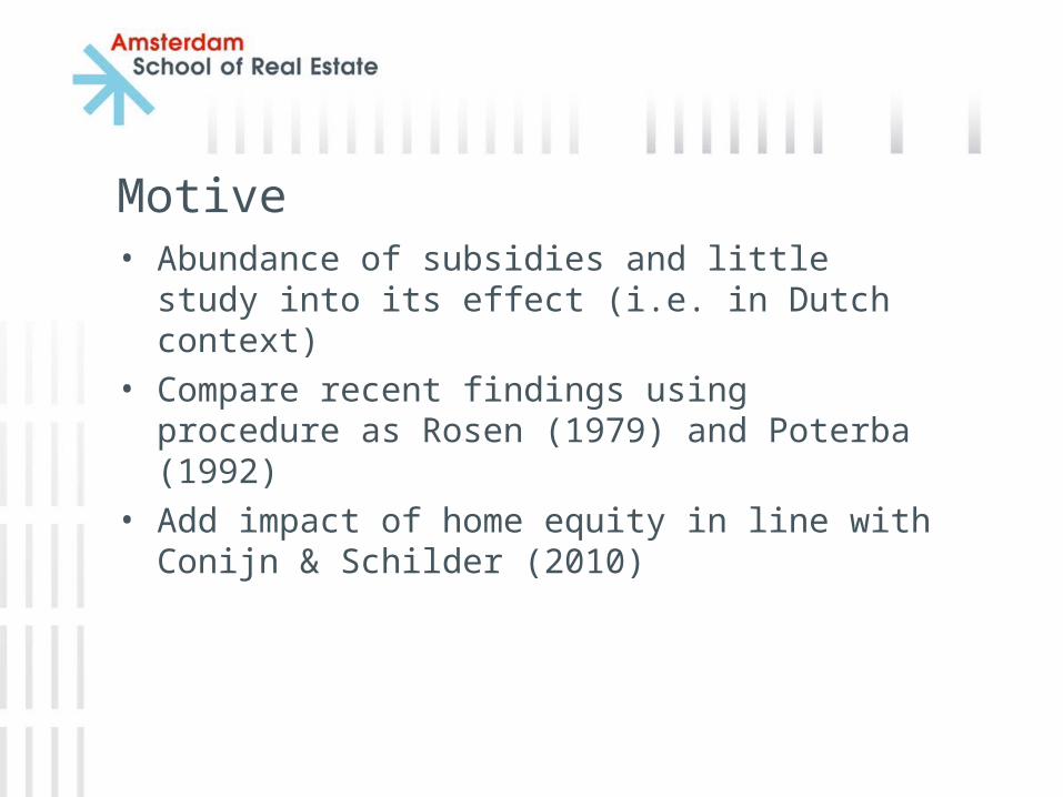
Context: housing market
Owner RenterAbsolute 3.83 3.30Relative 54 46
Housing association Private landlord Other TotalRegulated 2,4 0,3 0,3 3,0Non-regulated 0,1 0,1 0,0 0,2Total 2,4 0,4 0,4 3,2
Context: subsidiesOwner-occupier
- Mortgage interest deductibility- Tax exemption of capital gains / home equity
Renter- Housing allowance (low income only)- Regulated rents (implicit subsidy: all renters)
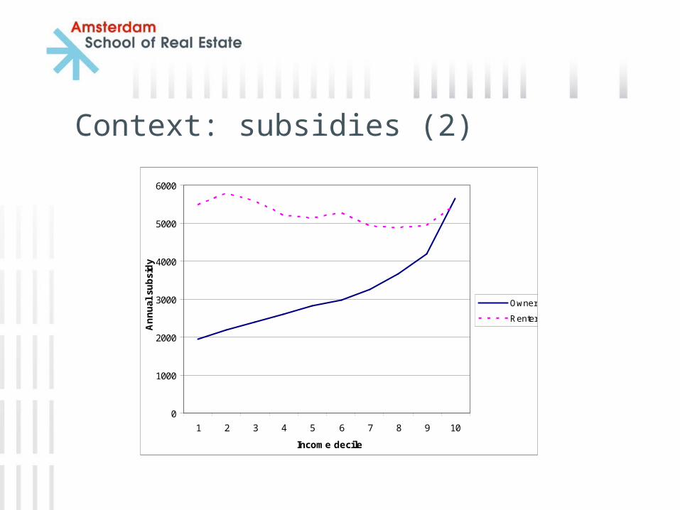
Context: subsidies (2)
0
1000
2000
3000
4000
5000
6000
1 2 3 4 5 6 7 8 9 10
Income decile
An
nu
al s
ub
sid
y
Owner
Renter
Welfare implications• Distorted housing consumption from subsidies
• Koning et al. (2006): 1 bln (owners only)
• Romijn & Besseling (2008): 2.75 bln (renters only)
• Donders et al. (2010): 3.7 – 7.4 bln (all – depending on scenario)

Welfare implications (2)
Inkomensdeciel
% huur
5855
46
1981199020022006
90%
80%
70%
60%
50%
40%
30%
20%
10%
0%1 2 3 4 5 6 7 8 9 10

Research issues• National or regional markets?
• Estimating demand curve in regulated market
• Home equity
• Sample selectivity
DataWoON 2006
• Cross-section of Dutch households
• Questionnaire
• n = 64.005
• Data on household characteristics, stated preferences, current consumption etc.
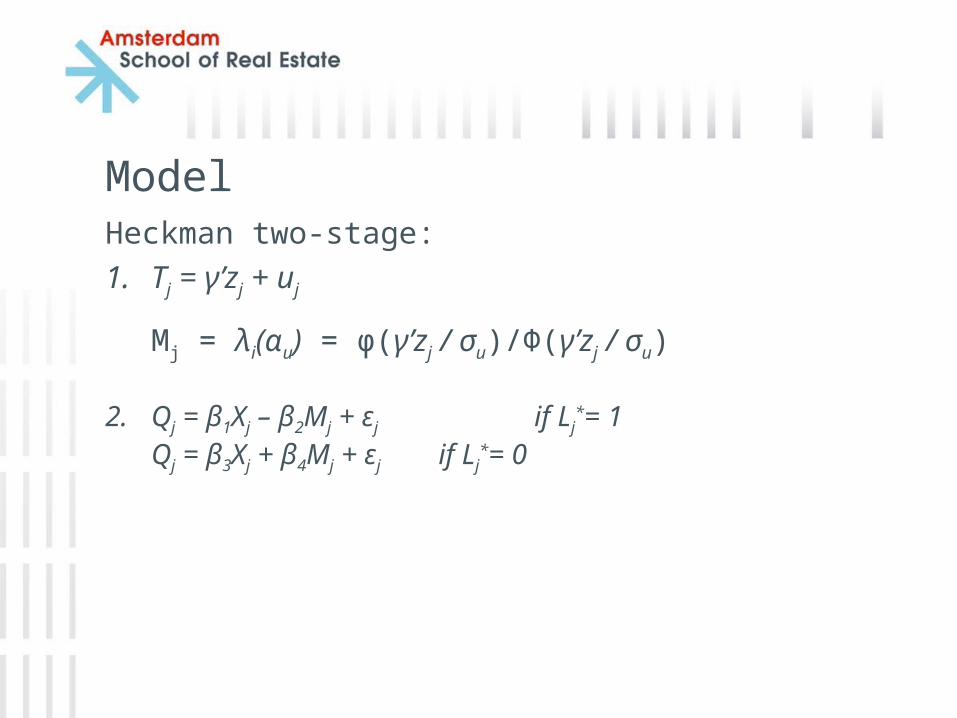
ModelHeckman two-stage:
1. Tj = γ’zj + uj
Mj = λi(αu) = φ(γ’zj / σu)/Φ(γ’zj / σu)
2. Qj = β1Xj – β2Mj + εj if Lj*= 1
Qj = β3Xj + β4Mj + εj if Lj*= 0
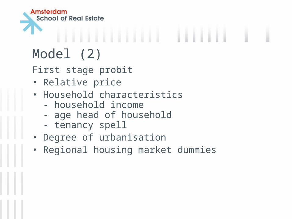
Model (2)First stage probit• Relative price• Household characteristics
- household income - age head of household- tenancy spell
• Degree of urbanisation• Regional housing market dummies
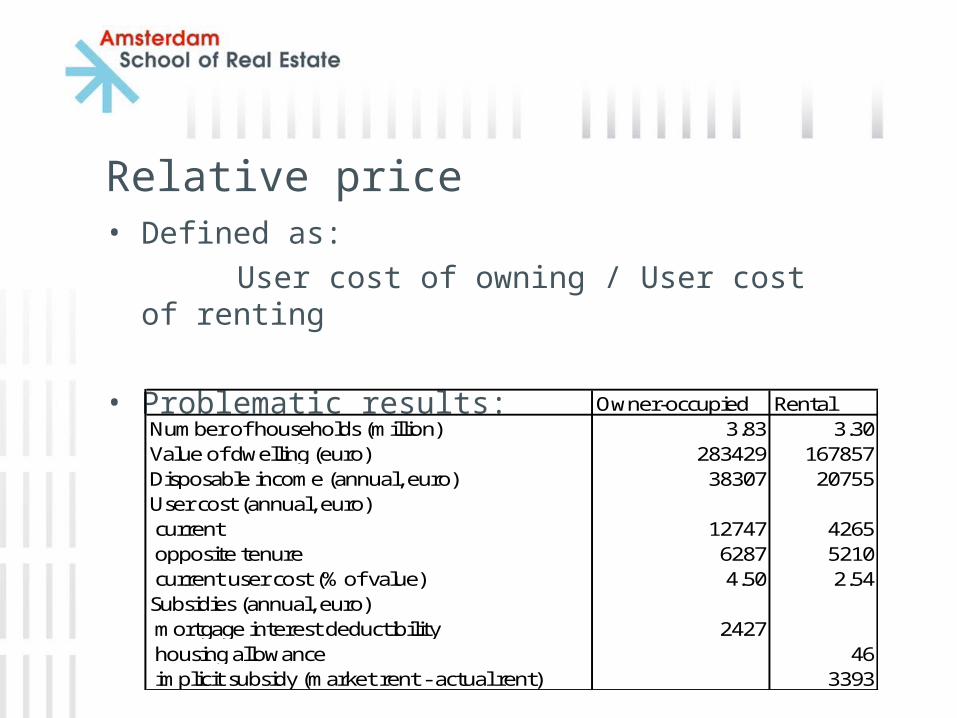
Relative price• Defined as:
User cost of owning / User cost of renting
• Problematic results:Owner-occupied Rental
Number of households (million) 3.83 3.30Value of dwelling (euro) 283429 167857Disposable income (annual, euro) 38307 20755User cost (annual, euro) current 12747 4265 opposite tenure 6287 5210 current user cost (% of value) 4.50 2.54Subsidies (annual, euro) mortgage interest deductibility 2427 housing allowance 46 implicit subsidy (market rent - actual rent) 3393

Model (3)Second stage OLS• User cost per housing service• Household characteristics
- Household income- Home equity- Household composition- Tenancy spell- Inverse Mills’ ratio
• Degree of urbanisation
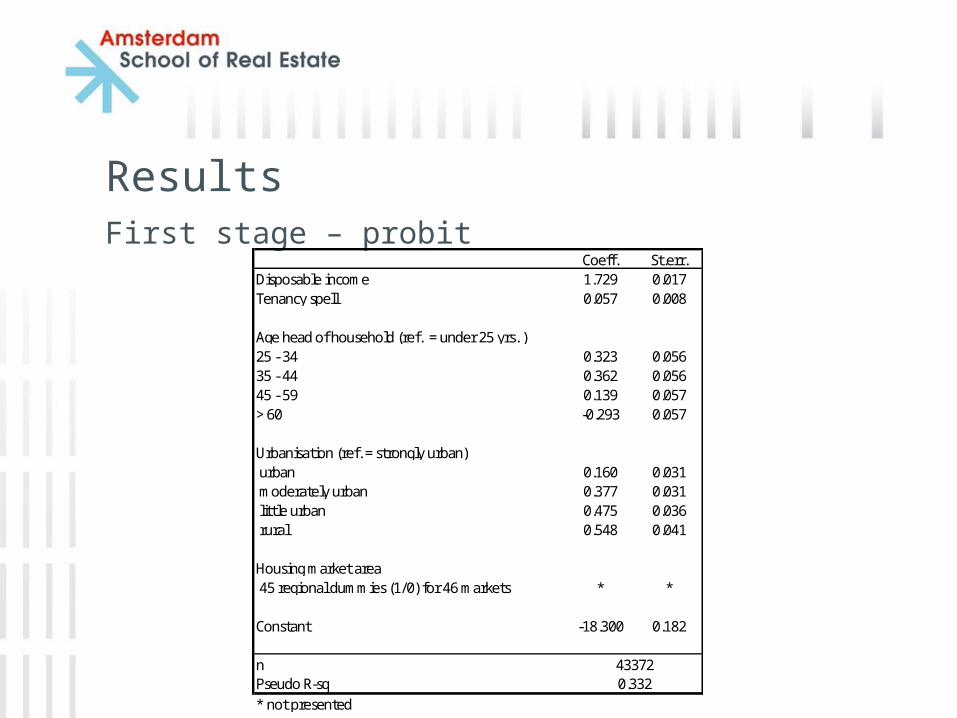
ResultsFirst stage – probit
Coeff. St.err.Disposable income 1.729 0.017Tenancy spell 0.057 0.008
Age head of household (ref. = under 25 yrs. )25 - 34 0.323 0.05635 - 44 0.362 0.05645 - 59 0.139 0.057> 60 -0.293 0.057
Urbanisation (ref. = strongly urban) urban 0.160 0.031 moderately urban 0.377 0.031 little urban 0.475 0.036 rural 0.548 0.041
Housing market area 45 regional dummies (1/0) for 46 markets * *
Constant -18.300 0.182
nPseudo R-sq* not presented
433720.332
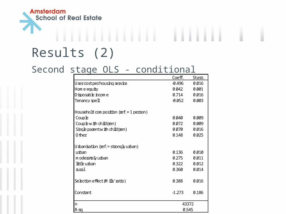
Results (2)Second stage OLS - conditional
Coeff. St.err.User cost per housing service -0.496 0.016Home equity 0.042 0.001Disposable income 0.714 0.016Tenancy spell -0.052 0.003
Household composition (ref. = 1 person) Couple 0.040 0.009 Couple with child(ren) 0.072 0.009 Single parent with child(ren) 0.070 0.016 Other 0.148 0.025
Urbanisation (ref. = strongly urban) urban 0.136 0.010 moderately urban 0.275 0.011 little urban 0.322 0.012 rural 0.360 0.014
Selection effect (Mills' ratio) 0.388 0.016
Constant -1.273 0.186
nR-sq
433720.545
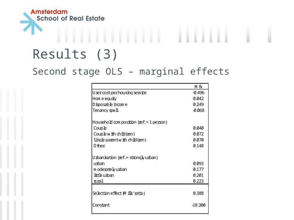
Results (3)Second stage OLS – marginal effects
MfxUser cost per housing service -0.496Home equity 0.042Disposable income 0.249Tenancy spell -0.068
Household composition (ref. = 1 person) Couple 0.040 Couple with child(ren) 0.072 Single parent with child(ren) 0.070 Other 0.148
Urbanisation (ref. = strongly urban) urban 0.093 moderately urban 0.177 little urban 0.201 rural 0.223
Selection effect (Mills' ratio) 0.388
Constant -18.300
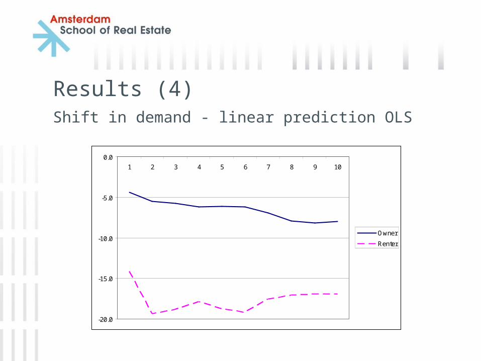
Results (4)Shift in demand - linear prediction OLS
-20.0
-15.0
-10.0
-5.0
0.0
1 2 3 4 5 6 7 8 9 10
Owner
Renter
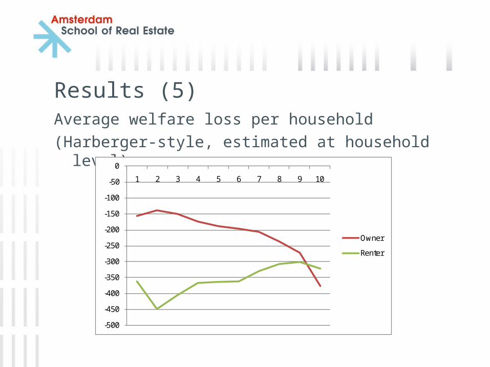
Results (5)Average welfare loss per household
(Harberger-style, estimated at household level)
-500
-450
-400
-350
-300
-250
-200
-150
-100
-50
0
1 2 3 4 5 6 7 8 9 10
Owner
Renter
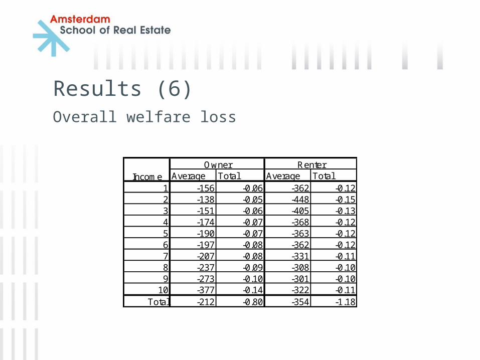
Results (6)Overall welfare loss
Average Total Average Total1 -156 -0.06 -362 -0.122 -138 -0.05 -448 -0.153 -151 -0.06 -405 -0.134 -174 -0.07 -368 -0.125 -190 -0.07 -363 -0.126 -197 -0.08 -362 -0.127 -207 -0.08 -331 -0.118 -237 -0.09 -308 -0.109 -273 -0.10 -301 -0.10
10 -377 -0.14 -322 -0.11Total -212 -0.80 -354 -1.18
RenterIncome
Owner

Conclusions• Significant welfare losses in the housing market
• Caused by disrupted consumption following incentives from housing subsidies
• Effects larger in rental sector than in owner-occupied sector