The Effects of Capital Subsidization on Israeli Industry

The Effects of Capital Subsidization on Israeli Industry

Introduction

Capital subsidization has been at the center of industrial policy in Israel over the

last thirty years. Its declared objectives were to encourage economic growth and

employment, as well as to improve the balance of payments and disperse the population

throughout the country. Government intervention focused on the Law of

Encouragement of Capital Investments (1959; here after “the Law”). This Law was

amended periodically1, but since 1968 it has granted four main types of investment

subsidies to “approved enterprises”: grants, loans with low rates of interest (often

negative real rates), accelerated depreciation, and other tax concessions on income

derived from the investment2.

Similar industrial strategy programs are supported by many countries. Factor

subsidies have been used extensively in European countries as important policy

instruments, usually in an attempt to reduce regional unemployment differentials

(Amstrong & Taylor (1985), Yuill et al (1989), Holden & Swales (1993)). Most

developing countries provide fiscal incentives to encourage domestic and foreign

investment. These schemes subsidize significantly the use of capital and produce greater

capital intensity in manufacturing (Lim (1992)). Moreover, the committee on industrial

support policies in the OECD stresses that: “Industrial subsidies often present

1 Up to the year 1990 it was changed 39 times, because of problems of implementation or changes ininvestment needs.2 Investments in equipment were entitled to grants of about 35 to 40 percent in Development Zone A, 20percent in zone B and 0 - 5 % in the central areas. About 40 % of the value of total investments got loans,which were unlinked to inflation until 1981-2. The accelerated depreciation allowance for equipment wastwice the rate of the regular one, and that for structures - 4 times. Corporate tax for approved enterpriseswas 25% instead of the ordinary tax of 45% (foreign investors paid only 10%).

2

impediments to structural adjustments, distort resource allocation and engender

international frictions... Reducing such subsidies is crucial for improving the flexibility

of economies and for increasing international trade on a competitive basis” (OECD

(1990)).

Canada has had extensive experience with the subsidization of capital investment

for the purpose of regional development.3 The degree of government involvement

reached its height in 1982 when the Canadian Government created a new Department of

Regional Industrial Expansion (DRIE) with its own cabinet minister; a department

whose mandate was to foster increased industrial activity in high unemployment regions.

While the level of subsidization has declined in recent years, as late as 1995 one billion

Canadian dollars was spent on industrial subsidies by the Canadian federal government

(Canadian Tax Foundation (1996)).

The leading principle embodied in the Law in Israel was the favoring of

industrial plants located in designated development zones, particularly in Galilee and the

Negev, and/or the encouragement of exports. Other general factors taken into

consideration in the selection of projects, as declared by the Investment Authority, were

the potential for creating employment, for contributing to the development of the area,

and for profitability. A rough estimate4 shows that the average subsidization embodied

in grants and loans alone, in the period 1970-1975, was some 20 percent of total

investment in industry (including investments that received no subsidies). It reached

31% in 1975-80; and declined again to 15% - 20% in the eighties. One should keep in

mind that these averages include many firms with subsidies of more than 50% of their

investments; for example - a firm investing in development area A in the second half of

3 The Atlantic Provinces are Canada’s own version of Israel’s development area A. 4 For a detailed explanation, see Bank of Israel Annual Report 1988, pp. 37-43, 156.

3

the 1970s received an ex-post subsidy of some 60 percent only by grants and loans. In

addition, there are other benefits to investing which are not included in the estimates

presented here.5

The main framework of the system was still functioning in the first half of the

nineties, but some alternative routes of subsidization were added: mainly government

guaranties for loans and income tax exemption for 10 years. The tax benefits were

estimated by the State Revenues department of the Finance Ministry, to approach

approximately $300m in 1997. Most investors (three-quarters of them) preferred the

grants however. Approved investments entitled to subsidies in the last few years, (since

1990) accounted for some 31% of total industrial investments. The sum of actual grants

plus an estimate of the value of the alternative benefits averaged an annual 42% of the

value of approved investment in this period.6 Grants were also the most widely used

financial instruments in OECD countries. Many of these countries also used

government loans and tax concessions in their regional policies (OECD (1990)).

It has been claimed that capital subsidization, along with high taxes on labor,

encouraged capital-intensive industries, decreased capital utilization, caused

inefficiency, and distorted the allocation of resources in the economy. Generally

speaking, the subsidization system in Israel and elsewhere is full of discriminations: by

destination - between production for local markets and exports; by ownership - between

local and foreign investors; by industry - manufacturing industry versus services; by

area, by type of asset (equipment versus structures), and in practice, also by size.

As we demonstrate below, the Law caused investors to prefer physical capital to

5 Among the benefits not included are the loan guarantees that were available to firms in the 1990s asan alternative to grants.6 The official grant rate in development area A (where 75% of the approved investment was concentrated)was 38%. Accordingly, one firm (Intel) recently received approval for a grant of 600(!) million dollars

4

labor, and to establish capital-intensive plants in development areas that were profitable

to the investor but not necessarily to the economy. Cheap capital, sometimes at a cost of

less than half its value, apparently resulted in over-investment, partial utilization of

machinery and equipment in industry, and unbalanced growth in the economy.

The development areas did not necessarily benefit over the long term. The high

rate of subsidization brought more investments but mainly for short periods. Many of the

subsidized plants in these areas closed down a short time after the subsidization period

ended (Lavy (1994))7. This result suggests that the subsidy scheme is not achieving its

declared aims - participation in government subsidy schemes in order to set up new

firms in developing towns appears to be associated with shorter life span of firms.

Similar developments have also been observed in other countries.

It is difficult to conclude that the Law achieved substantial net development in

the southern and northern regions (mainly constituting development area A). Although

the estimates show an increase in the rate of employment in these areas up to the

beginning of the eighties8, we cannot tell how much is due to other reasons. (To what

extend does the number of employees in the Dead Sea Works, for example, depend on

investment subsidization?)

The Law tried to achieve simultaneously two policy objectives that do

not necessarily coincide: preventing market failures and promoting specific areas. In

addition, the government used a very flexible map and definitions for the development

areas, which also changed under political pressure9. Although market failures are

for its intended investment of $1.6 billion, in Kiryat-Gat, in the next several years. 7 As found in a comprehensive study by D. Schwartz (1990, 1993)

8 From 21% out of total employees in the business sector in the sixties to 25% in the eighties and 26% inthe last years. 9 For example, a specific project in Haifa was included in development area A for a short while in order tosubsidize it.

5

characteristic of small firms, the government preferred large firms which could deal with

the bureaucracy and exert higher pressure on the politicians.

The overall effect of this subsidy system on the efficiency and productivity of

industrial firms is the ultimate purpose of this study, which is conducted at the

establishment level. We try to quantify the effect of capital subsidies on the productive

efficiency of firms, utilizing the production function framework. On the one hand, the

subsidy reduces the cost of capital, leading to a substitution of capital for labor

(allocative inefficency) and perhaps inducing technical inefficiency as well. On the

other hand, the subsidy, because it reduces the cost of capital, lowers the cost of

production (as long as input substitution occurs). The firm can thus lower its price and

expand output and the demand for labor. While the ultimate goal of our study is to try to

evaluate the capital subsidy policy by comparing some of the possible benefits of the

subsidization system such as output and employment growth with its costs, in this first

paper we consider only the efficiency costs.

In the next section we will present a short description of the unique data set that is used

for this study. The methodology is described in section 3, followed in section 4 by the

empirical results. In the first part of section 4, descriptive statistics that provide evidence

concerning the characteristics of firms that receive capital subsidies will be presented. In

the second part of section 4 production function estimates of the efficiency effects of

subsidies will be provided. Section 5 will conclude the paper with some preliminary

policy recommendations and suggestions for further research.

2. The Data

Three main surveys, conducted by the Central Bureau of Statistics, were used to

build the cross section - time series panel of firm data used in our study:

(1) The annual Industrial Surveys on incomes, expenditures, exports, labor inputs,

investments, and other related data on firms with five or more employees. It should be

mentioned that among the characteristics of the firm, the region in which the firm is

located is recorded, but unfortunately this is not always the case for individual plants.

6

The panel covers the 1990-1994 period, and includes approximately 2,000 industrial

firms that operated in this period.

(2) A Fixed Capital Stock Survey (as of January 1, 1992)10 was used to estimate the

firm’s capital stock by year of investment. A unique feature of this capital stock survey

is the fact that the amounts of capital grants are recorded in the same detail as the capital

investment. The survey is based on reports submitted to the tax authorities by the firms

in order to receive depreciation allowances. It includes detailed data on capital assets by

type and year of acquisition.11 Our data base is a representative unbalanced sub-sample

of the above mentioned annual Survey, and includes about 620 firms. Constant dollar

capital stock and capital grants at the individual firm level were generated for the period

1990-1994. Estimates for years other than 1992 were obtained by using the Survey data

as a benchmark, together with annual investment data, annual grants data, and

appropriate price deflators; utilizing the perpetual inventory method of capital stock

accumulation.

(3) R&D surveys, conducted by the CBS annually since 1969, which cover expenditures

on R&D investment, labor input (by education) and subsidies to R&D. Censuses were

conducted in 1979, 1984, and 1990. The R&D capital stock for every firm was

estimated from these data, assuming a depreciation rate of 1\7, and using the perpetual

inventory procedure used to estimate fixed capital services for the years 1990,91,93,94.

Additional information - on subsidization rates, taxes, and detailed geographic

coverage of the development areas - was collected mainly from official publications of

10 Only two other Capital Surveys were conducted in Israel, one for 1968 and the other for 1982, becauseof its complexity and unusual measurement difficulties. 11 Some firms were excluded from the panel because of statistical problems estimating their capital stock.For the regression analysis we used information on 620 firms, out of the original survey of 727 firms,after elimination of firms with outlying - probably wrong - basic data and firms which did not return thecapital stock survey questionaire.

7

the Investment Authority. See Regev (1993) for a detailed description of the

longitudinal panels, part of which we are using in this paper.12

The firm data include the values of output and intermediate inputs in current and

constant prices. The estimates of the appropriate price indexes were calculated for some

100 sub-branches of the industrial sector using various sources of price data. In some

cases there was an even finer detailed breakdown of the price data. The overall index of

output prices for every branch is a weighted average of export prices and the wholesale

price index for sales in the domestic market. The weights used were the real sales to the

different destinations.

The price index of intermediate inputs (materials) is based on information

regarding imports and purchases from local production as calculated in the CBS Input-

Output Tables. The data are classified here into some 200 sub-branches of commodities

and services. The overall materials price index is an average of import and local

production prices weighted by 1991 values from the input-output table for that year.

The main characteristics of the firm that serve as heterogeneity controls in the

production functions are: the size of the firm (measured by the labor input), a dummy

variable for mobility (entry and exit of firms), the qualities of labor and capital inputs

(for detailed definitions and explanations of the quality calculations see Regev (1997)),

the intensity of R&D activity, the utilization of capital by shift work, the ownership

sector (e.g., public sector, Histadrut), the industry the firm belongs to, and the year of

activity.

12 For additional descriptions of the characteristics of the data base used in this study see our previouspublications which utilize these data (Bregman, Fuss and Regev (1991,1995)).

8

3. The Methodology

The main purpose of this study is to investigate the effect of capital

subsidization on the production structure and efficiency in the Israeli manufacturing

industries. A firm will invest over time in a number of vintages of capital. The

amount of investment in vintage i will depend on the user cost of capital, which in

turn will depend on the extent of subsidization current at the time the investment is

made. It is these vintage investments and subsidies we observe in our data set. From

these data we wish to construct an aggregate capital stock and a measure of the

intensity of subsidization embodied in the capital stock in use by a particular firm at a

point in time (t).

According to the theory of aggregation (Leontief (1947a,b), Fisher (1965),

Hulten (1990)), an aggregate capital stock Kt exists if the relative marginal products

of vintages i and k are independent of the inputs outside of the aggregate. In this case

the aggregate stock of capital can be calculated as

Kt = It,0 + ∑ φt-i It,i (1)

where

It,0 = new capital investment13

It,i = capital investment of vintage i (in efficiency units) surviving to the beginning of year tφt-i = marginal product of vintage i capital / marginal product of new capital = MPt,i / MPt,t ,

and the summation is over all surviving vintages of capital (i>0).

According to the neoclassical model of capital accumulation (Jorgenson

(1963), Hall and Jorgenson (1967)), the firm will expect to maximize the present

13 Kt is defined as the aggregate capital stock at the beginning of period t. Hence It,0 is investment

9

value of profits from a particular vintage i investment by investing up to the point

where the value of the marginal product of capital is equal to the user cost of capital

ci 14,

pi MPi,i = ci (2)

MPi,i = ci /pi (3)

where pi is the output price at time i.

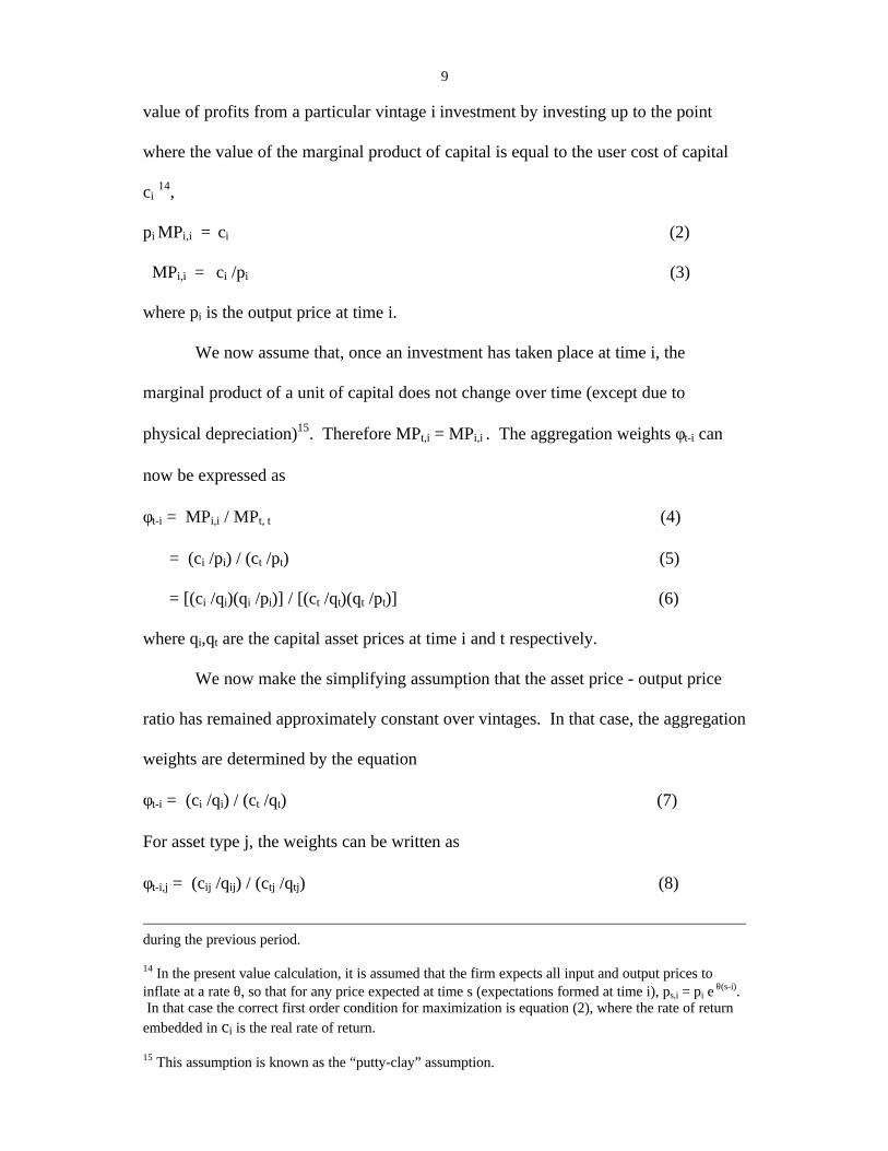
We now assume that, once an investment has taken place at time i, the

marginal product of a unit of capital does not change over time (except due to

physical depreciation)15. Therefore MPt,i = MPi,i . The aggregation weights φt-i can

now be expressed as

φt-i = MPi,i / MPt, t (4)

= (ci /pi) / (ct /pt) (5)

= [(ci /qi)(qi /pi)] / [(ct /qt)(qt /pt)] (6)

where qi,qt are the capital asset prices at time i and t respectively.

We now make the simplifying assumption that the asset price - output price

ratio has remained approximately constant over vintages. In that case, the aggregation

weights are determined by the equation

φt-i = (ci /qi) / (ct /qt) (7)

For asset type j, the weights can be written as

φt-i,j = (cij /qij) / (ctj /qtj) (8)

during the previous period.

14 In the present value calculation, it is assumed that the firm expects all input and output prices toinflate at a rate θ, so that for any price expected at time s (expectations formed at time i), ps,i = pi e

θ(s-i). In that case the correct first order condition for maximization is equation (2), where the rate of returnembedded in ci is the real rate of return.

15 This assumption is known as the “putty-clay” assumption.

10

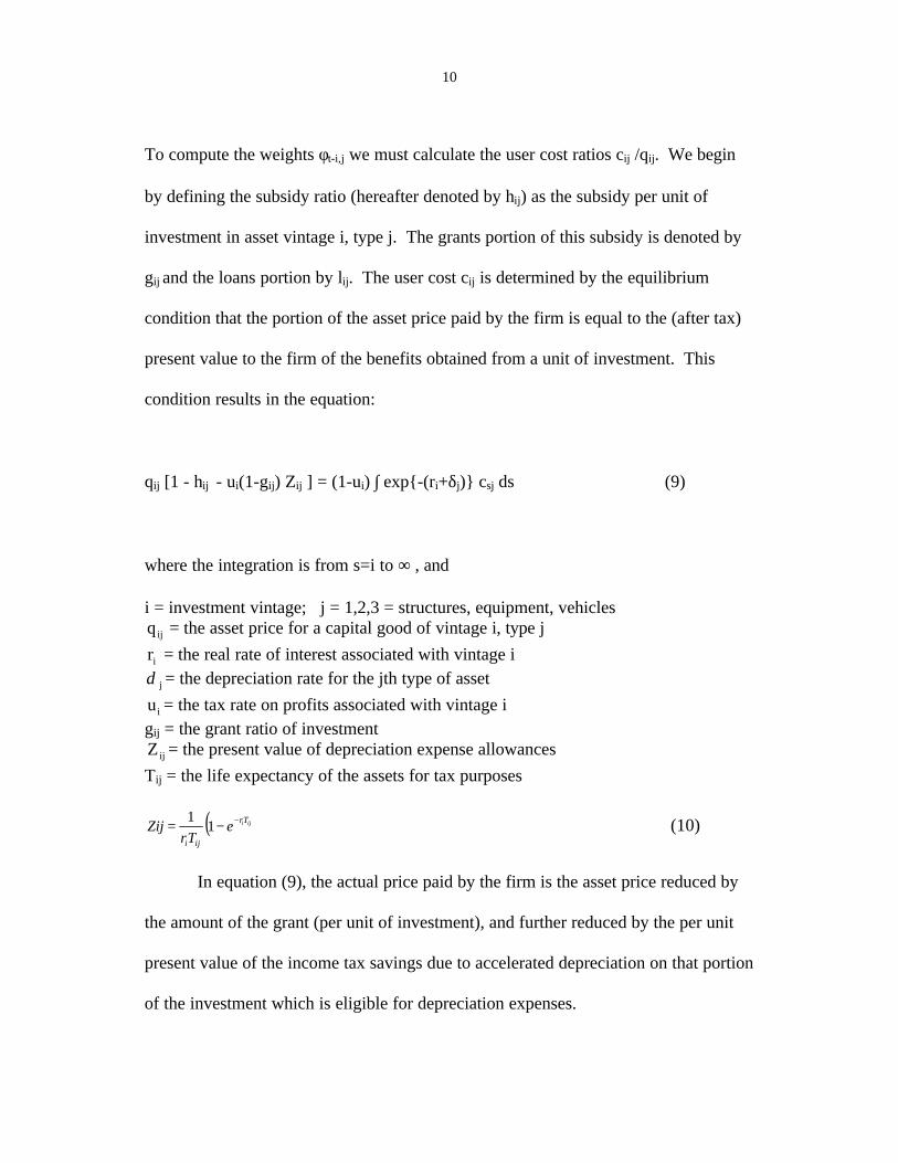
To compute the weights φt-i,j we must calculate the user cost ratios cij /qij. We begin

by defining the subsidy ratio (hereafter denoted by hij) as the subsidy per unit of

investment in asset vintage i, type j. The grants portion of this subsidy is denoted by

gij and the loans portion by lij. The user cost cij is determined by the equilibrium

condition that the portion of the asset price paid by the firm is equal to the (after tax)

present value to the firm of the benefits obtained from a unit of investment. This

condition results in the equation:

qij [1 - hij - ui(1-gij) Zij ] = (1-ui) ∫ exp{-(ri+δj)} csj ds (9)

where the integration is from s=i to ∞ , and

i = investment vintage; j = 1,2,3 = structures, equipment, vehiclesq ij = the asset price for a capital good of vintage i, type j

ri = the real rate of interest associated with vintage iδ j = the depreciation rate for the jth type of asset

u i = the tax rate on profits associated with vintage igij = the grant ratio of investmentZ ij = the present value of depreciation expense allowances

Tij = the life expectancy of the assets for tax purposes

( )ijiTr

iji

eTr

Zij −−= 11 (10)

In equation (9), the actual price paid by the firm is the asset price reduced by

the amount of the grant (per unit of investment), and further reduced by the per unit

present value of the income tax savings due to accelerated depreciation on that portion

of the investment which is eligible for depreciation expenses.

11

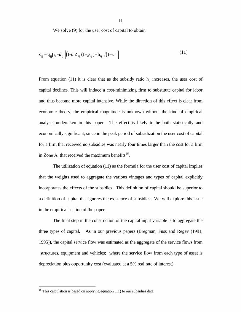
We solve (9) for the user cost of capital to obtain

( ) ( ) ( )[ ]c q r + 1-u h uij ij i j i ij ij i= − − −δ Z g ij( )1 1 (11)

From equation (11) it is clear that as the subsidy ratio hij increases, the user cost of

capital declines. This will induce a cost-minimizing firm to substitute capital for labor

and thus become more capital intensive. While the direction of this effect is clear from

economic theory, the empirical magnitude is unknown without the kind of empirical

analysis undertaken in this paper. The effect is likely to be both statistically and

economically significant, since in the peak period of subsidization the user cost of capital

for a firm that received no subsidies was nearly four times larger than the cost for a firm

in Zone A that received the maximum benefits16.

The utilization of equation (11) as the formula for the user cost of capital implies

that the weights used to aggregate the various vintages and types of capital explicitly

incorporates the effects of the subsidies. This definition of capital should be superior to

a definition of capital that ignores the existence of subsidies. We will explore this issue

in the empirical section of the paper.

The final step in the construction of the capital input variable is to aggregate the

three types of capital. As in our previous papers (Bregman, Fuss and Regev (1991,

1995)), the capital service flow was estimated as the aggregate of the service flows from

structures, equipment and vehicles; where the service flow from each type of asset is

depreciation plus opportunity cost (evaluated at a 5% real rate of interest).

16 This calculation is based on applying equation (11) to our subsidies data.

12

4. Empirical Results

a. Descriptive Statistics

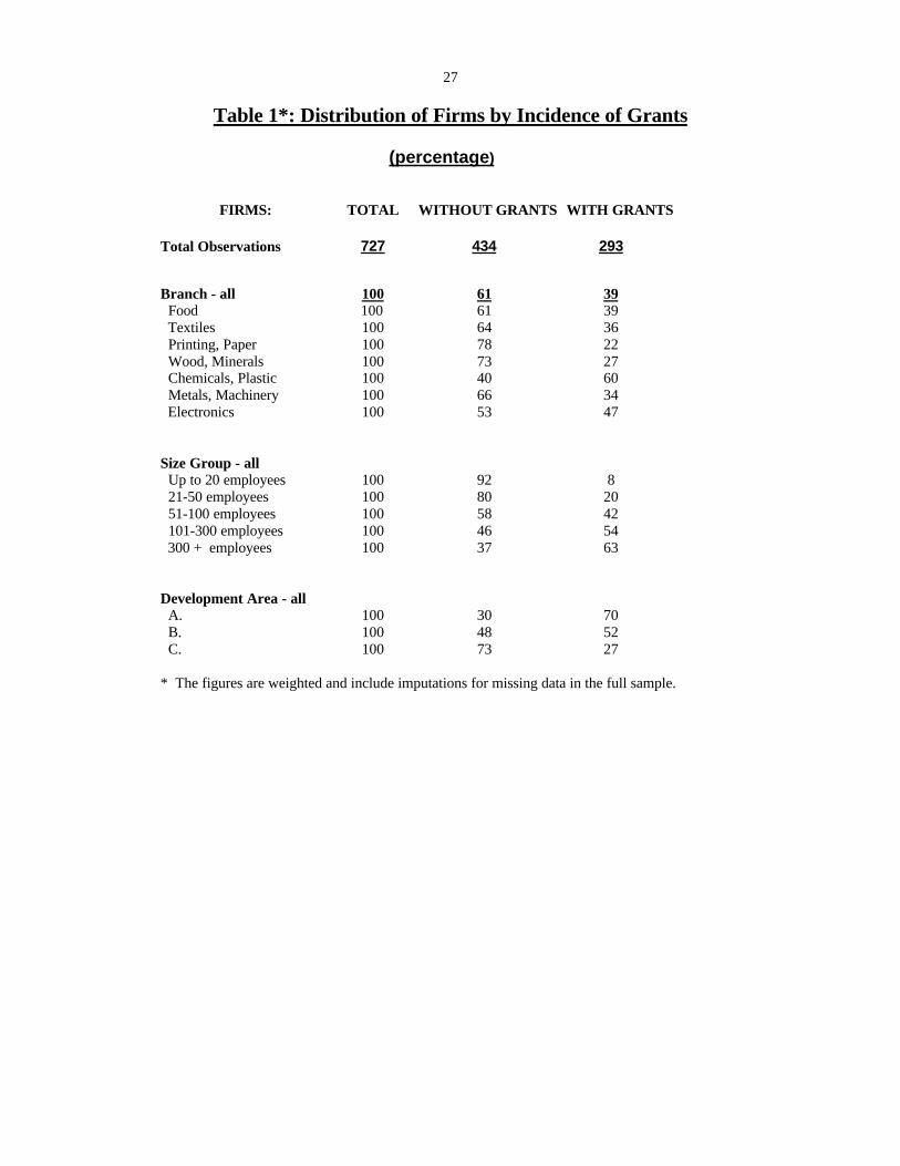
Tables 1 to 3 present some characteristics of the firms, sorted by the incidence of

capital subsidies. The data pertain to the years 1990-94. The descriptive statistics are

based on the full sample of 727 firms, where imputations were used to construct any

missing data. The data for these 727 firms were then expanded to the total population of

industrial firms in the Israeli economy using Central Bureau of Statistics expansion

factors (based on employment), in order to represent more accurately the whole of Israeli

industry. All data with the exception of the first row of Table 1 are after expansion. By

way of contrast, the regressions that follow (Tables 4 and 5) do not employ this

weighting procedure and include only the sample of 620 firms for which missing data

imputations were not necessary.

From Table 1 it can be seen that 293 of the 727 firms (40%) received grants for

capital in use as of the date of the observation. After expanding this sample of 727

firms, we obtain the result that over the 1990-94 period, 39% of the labor force in Israeli

industry worked for firms that utilized capital partially financed by grants. These

employment shares vary from a low of 22% in Printing and Paper to a high of 60% in

Chemicals and Plastic. As the size of firm increases, the share increases. As expected,

the highest percent of employment in firms with grants (70%) is in development area A,

with the next highest being development area B (52%). Perhaps surprising is the

sizeable percentage of firms in development area A without grants (30%), and the

percentage of firms in development area C with grants (27 %).

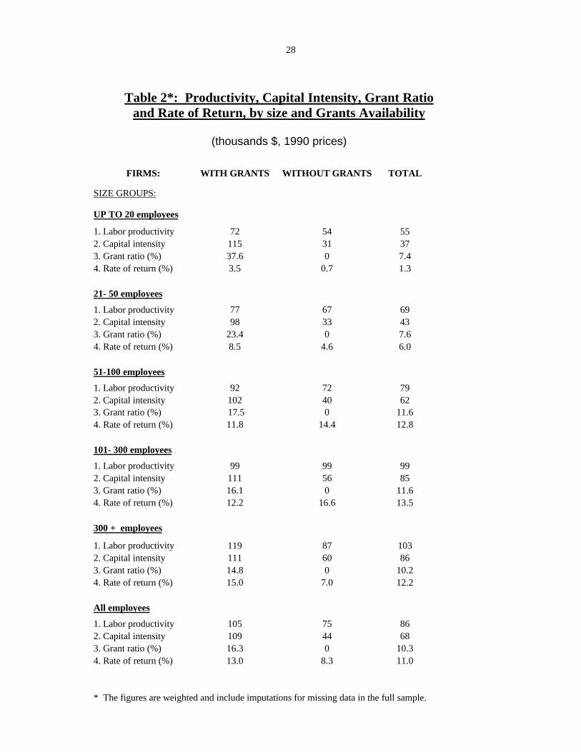
Table 2 provides a number of relevant economic indicators by size and incidence

13

of grants. The results in this table show that while there is some variation by size group,

on average, those firms who received grants had higher labor productivity, were more

capital intensive (higher capital/labor ratio) and had higher rates of return on capital.

The fact that firms with grants had higher labor productivity and were more capital

intensive suggests these firms were substituting cheaper capital for labor. The higher

labor productivity is not an indicator of greater efficiency, since a number of

characteristics (including capital intensity) varied systematically between firms with and

without grants. We will take this variation into account in our regression analysis (Table

4), where we demonstrate that firms with grants were actually less efficient.

The fact that firms with grants had, on average, higher rates of return on capital

stock is surprising. It is particularly surprising since the calculation does not take into

account the leverage enjoyed by firms with grants who finance only a portion of their

capital stock. We will return to this issue below.

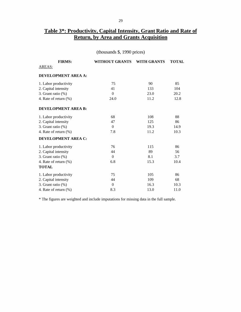
Table 3 highlights the differences in economic indicators among development

areas. Firms with grants have higher labor productivity and are more capital intensive

than firms without grants, regardless of area. With the exception of the anomalous result

in development area A17, firms with grants had higher rates of return than firms without

grants. Once again, the effective differences are understated since the leverage effects

on rates of return are ignored.

The comparative rates of return suggest that some segments of the subsidization

policy have been unnecessary, or at least too generous. In particular, consider

development area C. In this area, the issue of locating plants in underdeveloped regions

to stimulate employment is not at issue. The higher rates of return earned by firms that

17 The sample in this cell is small (42 firms), and the result is influenced by several firms with veryhigh calculated rates of return (over 1000%!) However when we remove the most unusual rates of

14

received grants than those that did not is indicative of the possibility of unnecessary

subsidization.

b. Construction of Alternative Subsidy Variables

As noted in the data section of this paper, the grants portion of the subsidy (gij)

for every firm is recorded in the Capital Stock Survey. The loans portion (lij) was

estimated by matching the individual observations with the terms of the loans specified

in the Law. The terms depend on the time and location of the investment, and whether

the firm qualifies as an exporter. This information is available from the data on firm

investments and characteristics. The actual subsidy embodied in the loan depends on the

nominal rate of interest charged, the nominal rate of interest prevailing in the market,

expected inflation during the payback period of the loan, and on the length of this loan

period. Our general approach to using this information to calculate the loan subsidy is

similar to that used in Litvin and Meridor (1983), Bregman (1985), and Bar-Nathan

(1989).

There are two ways in which the subsidy data was used. Section 3 of this paper

presents a theoretical model of the impact of subsidies based on an explicit application of

the neoclassical investment literature. This model was applied to the data. However,

before applying that model we first investigated a more ad hoc formulation. For each

firm at each point of time, each surviving investment was multiplied by the subsidy

ratio18 and aggregated to provide data on the proportion of the capital stock which is

subsidized. This calculation was performed for both the grants data (which is actual

return observations, the high average rate of return of about 20% for these firms remains.18 At this stage of the research we calculated the subsidy ratio for every firm from data on totalinvestments for every period of time (vintage), by using weighted averages of the different ratios of thethree types of capital available to us (structures, equipment and vehicles). We will perform the

15

data) and the grants + loans data (a mixture of actual and estimated data). These

variables were used as characteristics of the firm to be included in an augmented

production function estimation similar to the heterogeneity controls approach of

Bregman, Fuss and Regev (1995) and Griliches and Regev (1995). In this case, the

capital input is constructed as if subsidies were not present19.

c. The Regression Results

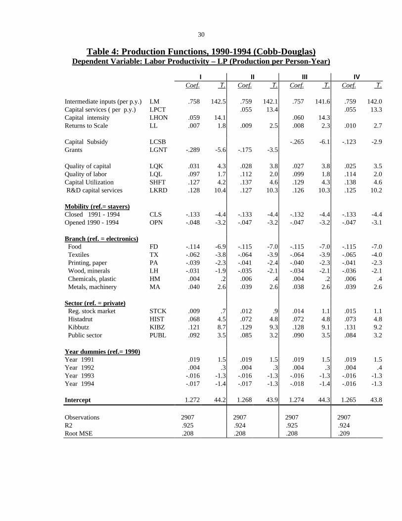
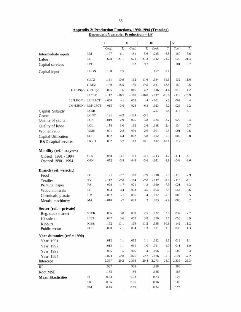
Table 4 contains OLS estimates of the parameters of the augmented Cobb-

Douglas production function.20,21 The more flexible translog function was also

estimated, but since the results were similar to the simpler Cobb-Douglas specification,

the translog results are relegated to an appendix (Appendix 2). The four columns of

results in Table 4 differ because of different versions of the subsidy variable and

different ways of measuring the capital input variable.22

In columns I and III, the capital input (LHON) is measured as the service flow

from the gross capital stock when the user cost of capital used to construct the aggregate

disaggregated calculations in later work. We do not expect the revised calculations to have a significantinfluence on the results. 19 To construct this variable, the aggregation theory outlined in section 3 was utilized, but theimplications of subsidies for the user cost of capital was ignored.20 Definitions of the neumonics representing the right hand side variables is contained in Appendix 1.21 In previous work with this data set we have also attempted to provide instrumental variableestimates to account for the possible endogeneity of the input variables. The various results have neverbeen sensitive to this change in estimation method, so we did not pursue this alternative in the currentpaper.22 A general issue with respect to all four columns is how to treat rental expenditures. The Israeli dataset has separate observations on the current dollar rental expenditures, unlike the U.S. manufacturingsurvey data that include rents in the intermediate inputs expenditure data. There are three possibilities:(1) ignore the data, (2) include it in materials (for comparability with U.S. results), (3) include it incapital. In previous work we ignored the information. Here we include it in capital by assuming anannual return of 12.5% on rented capital (rented capital=8*real rents). This inclusion characterizesboth the regression results to follow and the previous descriptive statistics. A problem with theinclusion of rents in capital is that we have no data on grants associated with rented capital. We haveinvestigated all three possible treatments of rent and the regression results are not sensitive to thechoice.

16

capital is calculated ignoring the existence of investment subsidies.23 In columns II and

IV, the capital service flow variable (LPCT) is calculated by applying the user cost of

capital variable that includes the subsidy adjustment (equation (11)) to estimate the

capital service flow. By construction, since subsidies lower the cost of capital, they also

lower the estimated service flow from a given stock of capital. The interpretation is that

firms with access to subsidized (hence less expensive) capital will extend their purchases

of capital to capital with a lower marginal product and therefore the service flow from a

given capital stock will be reduced.

In columns I and II the subsidies variable is represented by the proportion of

(constant dollar) grants actually received as a proportion of the (constant dollar) capital

stock (GNT)24. An increase in this variable implies a greater degree of capital

subsidization. In columns III and IV the subsidies variable CSB is calculated by adding

to the numerator of GNT the calculated non-grant subsidies (loans, tax concessions)

described above. This variable (CSB) represents our estimate of the total subsidy to

capital as a proportion of capital25. It is a mixture of actual grants observed and our

calculation of the additional subsidies the firms were entitled to receive as a result of

having qualified for the subsidy program in one of the various categories. An increase in

CSB implies a greater degree of subsidization.

Before we proceed to discuss the subsidy results, we first discuss the other

results of interest in Table 4. Since these other results are not very sensitive to the

23 The gross definition of capital was used because the grants were calculated on a gross basis. When theproduction function was estimated without including the subsidy variables, the estimated structure wasinvariant to whether the gross or net definitions of capital were used.24 The variable used in the regression is LGNT = log (1+GNT). The empirical results suggested that thislogarithmic transformation was the preferred way to deal with the fact that the majority of firms (60%) didnot receive grants. For such firms GNT=0.25 Once again, the variable actually used in the regression is the logarithmic transformation LCSB = log(1+CSB).

17

different versions of subsidy and capital input variables used, we will use the results in

column I as representative.

First, constant returns to scale appears to be a reasonable description of the

technology (the scale elasticity is 1.0126). Increases in the quality of capital and the

quality of labor result in increases in labor productivity (or equivalently, increases in

output or efficiency of production). A unique variable that we have available is the

extent of shift work. This variable is a direct measure of capital utilization. Not

surprisingly, increases in the number of work-shifts within a twenty-four hour period has

a statistically significant positive impact on output through the more intensive utilization

of the capital stock.27

Investment in R&D capital has a significant impact on labor productivity.28,29

Firms that opened or closed during the period of our data sample had lower productivity

than continuing, established firms. During those years in our sample when these firms

operated, new firms were 4.7% 30 less productive, whereas firms that closed were 12.5%

less productive31. Several branches of industry had lower output per unit labor than the

26 Since all non-labor input variables and output are deflated by labor, 1+ the coefficient on the labor input(LL) measures returns to scale (excluding the impact of R&D).27 The estimated coefficient implies that a firm that moved from one shift to two shifts and doubled itsuse of labor and materials inputs would double output. Hence the utilization of capital would double.28 In our formulation R&D capital plays a role in the production process analogous to structures andequipment capital. The variable used in the regression is LKRD = log (1+KRD) since KRD =0 for manyfirms. Due to this formulation, the estimate .13 is not the estimate of the R&D elasticity. The elasticityestimate is .13*[KRD/(1+KRD)], which is equal to 0.07 at the mean value of KRD for those observationswhere KRD >0. By comparison, the elasticity for physical capital is 0.06.29 We also estimated the model with a “no R&D” dummy variable included. As was the case forGriliches and Regev (1995), we obtained a statistically significant positive coefficient, which iscounterintuitive. However, the change in specification had no impact on the coefficients associatedwith the subsidy variables. 30 Calculated as (exp(-.048) -1)*100.31 Whether firms close is not independent of their productivity, so there is a potential simultaneity biasassociated with the variable CLS. However, deleting CLS and OPN from the regressions in Table 4did not change the other coefficients. The fact that closed firms are less productive than other firmssuggests a possible selectivity bias in our sample which should be kept in mind. Firms that closed priorto 1990 are not observed in our sample. Much of the subsidization activity took place prior to 1990. Ifa disproportionate number of low productivity firms that failed after a short existence and hence closed

18

reference branch (electronics). These branches were food, textiles, printing & paper, and

wood & minerals. Of considerable interest is the fact that the Histadrut and Public

sectors, during the 1990-94 period, had higher productivity than the Private (reference)

sector. This is a reversal of the results for the 1979-83 period reported in Bregman, Fuss

and Regev (1995), and suggests that firms in these sectors have made important relative

improvements in productive efficiency in recent years32.

We now turn to an analysis of the subsidy results. We consider first the results

in column I, where subsidies are measured in terms of actual grants and the capital input

is not adjusted for the presence of subsidies. The coefficient on LGNT is significantly

negative, implying that subsidized firms produce less output per unit labor, ceteris

paribus. For subsidized firms, the mean of LGNT is 0.104 and the maximum value is

.597. Hence at the mean value, subsidized firms are 3.0%33 less productive than

unsubsidized firms. For heavily subsidized firms, the productivity shortfall ranges up to

15.8%34. The same calculations can be performed for the broader subsidy variable

LCSB. For subsidized firms, this variable has a mean of 0.184 and a maximum value of

0.620. From column III of Table 1 it can be seen that the corresponding productivity

shortfalls are 4.8% and 15.2% respectively. The productivity differential estimate is

somewhat higher for the average subsidized firm when a broader range of subsidies is

taken into account. For heavily subsidized firms, grants dominate the subsidy-ratio

calculation, so that the two ways of calculating the subsidy ratio produce more similar

results.

The calculations above do not distinguish between productivity effects due to the

prior to 1990 were subsidized firms, then we will underestimate the effect of subsidization onproductivity.32 The apparent efficiency advantage of the Kibbutz firms may be an artifact of the likelyunderreporting of the amount of labor used in production.

19

incentives created by the subsidy system and productivity shortfalls that are due to

technical inefficiency. Because subsidized capital is cheaper capital, subsidized firms

have a rational incentive to purchase additional lower productivity capital, so that for

such firms the flow of services from any observed capital stock should be lower. As

noted earlier, we have taken this incentive into account by constructing a capital input

variable (PCT) for which the capital service prices used as weights explicitly incorporate

the subsidy effects. The impact of this weighting procedure is to create a capital input

variable that is systematically lower for subsidized firms than the previous variable

HON. It is also equal to HON for firms that did not receive subsidies. We would expect

that the lower output observed for subsidized firms would at least in part be accounted

for by this revised capital input variable. If this variable is correctly specified, and the

only output-lowering effect of subsidization is the rational purchase of additional lower

productivity capital by subsidized firms, the use of LPCT35 in place of LHON should

wipe out the impact of the subsidy variable (LGNT or LCSB). Inspection of columns II

and IV demonstrates that this is not the case36.

The coefficients of LGNT and LCSB are substantially reduced (from -.289 to -

.175 and -.265 to -.123 respectively). Approximately 50-60% of the productivity

shortfall observed which is associated with capital subsidization is estimated to be

attributable to technical inefficiency, while the remainder is caused by the rational choice

33 Calculated as (exp(-.289*.104)-1)*100.34 Calculated as (exp(-.289*.597)-1)*100. 35 LPCT is the logarithm of PCT. LHON is the logarithm of HON.36 It has been suggested to us that the apparently lower output may be due to the fact that a singleindustry-specific output price is used to deflate the revenues of both subsidized and unsubsidized firms. If firms with lower cost capital passed on the lower costs in the form of lower prices, such a resultcould be the case. However, this would only occur if a pattern of market power existed such that unsubsidized firms did not have to lower their prices under competitive pressure from subsidized firms,and there is no reason to believe this pattern exists.

20

of firms, faced with relatively inexpensive capital, to overcapitalize.37

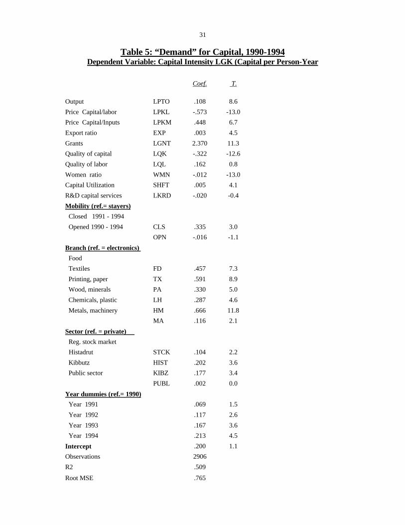
We now focus more closely on the question of overcapitalization. We do so by

estimating a capital intensity equation, where the dependent variable is the capital stock

per unit of labor and the subsidy variable used is the grants ratio38. Table 5 contains the

results of this estimation. We include relative input price and output variables, as well as

an extensive number of heterogeneity controls. While we are particularly interested in

the impact of subsidization on the capital intensity (capital stock per unit of labor), we

begin by considering the results pertaining to the other variables in the equation. The

capital- labor ratio is an increasing function of output, suggesting that the production

process is not homothetic.39 Capital and labor are estimated to be substitutes, whereas

capital and materials are estimated to be complements.

Firms that export a greater proportion of their output are more capital-intensive.

There is a tradeoff between quantity and quality of capital in satisfying production needs

(note the negative sign on the quality of capital). While capital intensity is estimated to

be an increasing function of the quality of labor (suggesting skilled labor-capital

complementarity), the effect is not statistically significant40. An interesting finding is

that capital-intensive production processes are associated with a lower proportion of

women in the workforce. Capital-intensive production processes are also associated

37 Although we utilize a time series – cross section data set, the above results of the effects of subsidiesare primarily determined by the cross section component of the data. We estimated both within (fixedeffects) and between versions of the model. For the within version, the subsidy effects wereinsignificant. The between version produced results similar to those reported in the paper. That thefixed effects version did not yield significant results is not surprising, since for any individual firmthere would not be much variation in the proportion of subsidized capital over the five year period ofour time series component. 38 An equation containing the subsidy ratio is not estimated since, due to its construction, this variableis endogenous with respect to the price of capital services, a variable which appears as a right-hand sidevariable.39 While this result contradicts the use of the Cobb-Douglas production function above, recall that we alsoestimated a translog function (which can be non-homothetic) with similar results regarding the productivityeffects of subsidies.40 Capital includes structures, equipment and vehicles. If the capital stock in this equation were

21

with more shift work - suggesting a not surprising desire to utilize capital more intensely

when it represents a larger proportion of production costs. R&D capital and physical

capital may be substitutes in production, but the effect is not statistically significant (see

the previous footnote for a possible rationale for lack of statistical significance).

Firms that closed sometime during 1990-94 are significantly more capital

intensive than continuing firms. We may be observing a period of low utilization of

capital just prior to closure. New firms are less capital intensive than continuing firms,

but not significantly so. There are significant differences in capital intensity among

branches, with electronics being the least capital intensive and chemicals & plastics

being the most capital-intensive. The Kibbutz sector appears to be a relatively capital-

intensive sector. This counterintuitive result is probably due to a systematic under-

reporting of the labor input, where labor hours supplied by Kibbutz members are not

always recorded. The individual year dummy variables demonstrate the phenomenon of

an increase over time in the capital intensity of production, ceteris paribus. This result is

consistent with labor-saving technical change. However, since an inter-temporal increase

in capital intensity is a basic feature of the data, the dummy variable coefficients

probably also reflect in part the impact of left-out variables and measurement errors.

We now come to the effects of grants on the capital intensity of production. It is

clear from the very significant positive coefficient of LGNT that subsidized firms are

more capital-intensive firms, even after accounting for the reduction in the capital

service price associated with subsidization. There are two possible explanations for this

result. First, we may have uncovered evidence of private allocative inefficiency on the

part of subsidized firms, although it should be noted that the capital used to construct the

intensity variable is the stock, not the service flow. Alternatively, the significant

restricted to equipment, a statistically significant effect would probably be found.

22

coefficients of the subsidy variables may be acting as controls for the mis-measurement

of the subsidy-adjusted capital service price. Since we cannot account for all the

subsidies obtained by subsidized firms, our estimate of the subsidized price may be too

high and therefore may not fully represent the rational incentive to use a more capital

intensive production process.

To this point we have concentrated primarily on documenting the productive

inefficiency associated with subsidized firms. But subsidizing firms is part of the Israeli

government’s policy of encouraging regional development of industry. It may be that

the only way to obtain regional development is to subsidize inefficient firms, who, as

part of the agreement will locate plants in development areas A and B as the pro quid pro

for obtaining the subsidies they need to compete. Hence we cannot, at least at this stage

of the research, determine whether firms are inefficient because they are subsidized, or

are subsidized because they are inefficient.41

One way to begin looking at this “chicken and egg” question is to compare the

profitability of subsidized firms with the profitability of unsubsidized firms. We saw

from Tables 2 and 3 that, on average, subsidized firms have higher rates of return than

unsubsidized firms. In fact, from Table 3 we can see that the rate of return for

subsidized firms in development area A exceeds that of unsubsidized firms in other areas

of Israel42. It does not appear that these firms have needed the subsidies to survive,

assuming the 1990-94 data is representative. That such firms appear to be both less

41 It has been suggested that an alternative explanation for the apparent inefficiency observed insubsidized firms is the fact that olim (new immigrants), who are probably less productive in their earlyyears in Israel, are concentrated in development areas and hence concentrated among the employees ofsubsidized firms. To explore this issue we estimated a specification that included a variable thatmeasured the proportion of the labor force that was made up of the new immigrants. While thisvariable had the expected significant negative coefficient, the coefficients of the subsidy variables wereunaffected. 42 Once again the peculiar result for unsubsidized firms in development area A clouds the issue and willneed to be understood.

23

efficient and more profitable remains a mystery as of this writing. The mystery only

deepens when one considers that the gap in rates of return will widen if only non-

subsidized capital were used in the denominator of the rate of return calculation.

5. Conclusions and Suggestions for Further Research

Perhaps for the first time, we have provided empirical evidence on the impact

that a program of subsidizing capital investment has on the nature of industrial

production. We have estimated, for the case of Israeli industry, the empirical realization

of the incentive to over-invest in subsidized (cheaper) capital. We have also found that

subsidized firms are likely to be technically inefficient - an effect which is separate from

the privately rational incentive to over-investment.

To this point we have only considered one side of the subsidy program - its costs.

In the next stage of the research we need to consider the possible benefits to the

economy of a program of subsidizing capital accumulation.

Because the subsidy ratio reduces the user cost of capital it lowers the cost of

production (as long as some degree of input substitution occurs). The firm can thus

lower price and expand sales, which is a growth-inducing effect that also increases the

demand for labor. This effect of subsidies on output-supply and labor-demand

relationships represents a potential benefit of subsidization that we need to try to

estimate. Whether the growth-inducing effect is greater than the adverse substitution

effect will help determine the net effect on the demand for labor (employment) which

results from the capital subsidy policy. Since the ultimate goal of government-supplied

capital subsidies is to provide additional employment at reasonable cost, calculation of

the net effect will be of most use to policy makers.

24

In principal, the calculation of the net benefit should also consider the

opportunity cost of the subsidies - the alternative public resource investments

that could have been undertaken using the same budget. The Law encouraged

investments in physical capital, while the rate of return for the economy may

have been much higher in investments in infrastructure and in R&D (a

reasonable assumption according to results of recent studies (Bregman &

Marom (1998), Griliches & Regev (1995))). Devoting more resources to

these alternative investments might have resulted in higher growth rates and

additional employment in the development areas. To the extent that greater

growth would have occurred, the use of public resources to fund physical

capital accumulation represents an additional degree of allocative inefficiency

which should not be ignored by policy makers when evaluating the subsidy

system.

25

References

Bar-Nathan, M. (1989), “Encouragement of capital incentives Law in Israel - ItsDevelopment and Results”, Bank of Israel, Research Department, mimeograph(Hebrew).

Bregman, A. (1985), “The Slowdown of Industrial Productivity - CausesExplanations, and Surprises”, Bank of Israel, Economic Review, No. 56.

Bregman, A., M. Fuss, and H. Regev (1991), “High-Tech and Productivity: Evidencefrom Israeli Industrial firms, European Economic Review 35, pp. 1191-1221.

Bregman, A., M. Fuss, and H. Regev (1995), “The Production and Cost Structure of Israeli Industry: Evidence from Individual Firm Data”, Journal of Econometrics,Vol. 65, No. 1, pp. 45 - 81.

Bregman, A. and A. Marom (1998), “Factors of Productivity in the IsraeliIndustry, 1960 - 1996”, Bank of Israel Research Department, Discussion PaperSeries 98.03, (Hebrew).

Canadian Tax Foundation (1996), The Finances of the Nation, Toronro, Canada

Fisher, F. (1965), “Embodied Technical Change and the Existence of an AggregateCapital Stock”, Review of Economic Studies, pp. 263-288.

Griliches, Z. and H. Regev (1995), “ Firm Productivity in Israeli Industry, 1979-1988”, Journal of Econometrics, Vol. 65, No. 1, pp. 175 - 203.

Hall, R.E. and D.W. Jorgenson (1967), “Tax Policy and Investment Behavior”,American Economic Review, June, pp. 391-414.

Holden, D. and J. K. Swales (1993), “Factor Subsidies, Employment Generation, andCost per Job: A Partial Equilibrium Approach”, Environment and Planning, 25(3),March, pp. 317-338.

Hulten, C. (1990), “The Measurement of Capital”, in E. Berndt and J. Triplett (eds.),Fifty Years of Economic Measurement, NBER Studies in Income and Wealth,Volume 54, University of Chicago Press, Chicago, Illinois, pp.119-152.

Lavy, V. (1994), “The Effect of Investment Subsidies on the Survival of Firms inIsrael”, The Maurice Falk Institute for Economic Research in Israel, Discussion PaperNo. 94.04, August.

Lim, D. (1992), “Capturing the Effects of Capital Subsidies”, The Journal ofDevelopment Studies Vol. 28 No. 4, July, pp. 705-716.

Leontief, W. (1947a), “A Note on the Interrelation of Subsets of Independent

26

Variables of a Continuous Function with Continuous First Derivatives”, Bulletin ofthe American Mathematical Society, pp. 343-50.

Leontief, W. (1947b), “Introduction to a Theory of the Internal Structure ofFunctional Relationships”, Econometrica, April, pp. 361-73. Litvin, U. and L. Meridor (1983), “The Grant Equivalent of Subsidized Investment inIsrael”, Bank of Israel, Economic Review, No. 54.

Mohr, M.F. (1986), “The Theory and Measurement of the Rental Price of Capital inIndustry- Specific Production Analysis: A Vintage Rental Price of Capital Model”, inA. Dogramaci, ed. Measurement Issues and Behavior of Productivity Variables,pp. 99-159.

Razin, E. and D. Schwartz (1992), “ Evaluation of Israel’s Industrial Dispersal Policyin the Context of Changing Realities”, The Economic Quarterly 153, December, pp.236-276.

Regev, H. (1993), “Industrial Enterprises Longitudinal Panels in Israel: Construction,Definitions and Use in Research”, Proceedings of the International Conference onEstablishment Surveys, American Statistical Association, Virginia.

Regev, H. (1997), “Innovation, Skilled Laabor, Technology and Performance inIsraeli Industrial Firms: 1982 - 1993”, The Maurice Falk Institute for EconomicResearch in Israel, Discussion Paper No. 97.06, May.

Schwartz, D. (1993), “The Implications of the Law for the Encourage of CapitalInvestment on Investment in Industry in Developing Areas”, Settlement Study Center,Rechovot (Hebrew).

OECD (1990), Subsidies and Structural Adjustment, Industrial Support Policiesin OECD Countries, 1982-1986. OECD, Paris, May.

27

Table 1*: Distribution of Firms by Incidence of Grants

(percentage)

FIRMS: TOTAL WITHOUT GRANTS WITH GRANTS

Total Observations 727 434 293

Branch - all 100 61 39 Food 100 61 39 Textiles 100 64 36 Printing, Paper 100 78 22 Wood, Minerals 100 73 27 Chemicals, Plastic 100 40 60 Metals, Machinery 100 66 34 Electronics 100 53 47

Size Group - all Up to 20 employees 100 92 8 21-50 employees 100 80 20 51-100 employees 100 58 42 101-300 employees 100 46 54 300 + employees 100 37 63

Development Area - all A. 100 30 70 B. 100 48 52 C. 100 73 27

* The figures are weighted and include imputations for missing data in the full sample.

28

Table 2*: Productivity, Capital Intensity, Grant Ratioand Rate of Return, by size and Grants Availability

(thousands $, 1990 prices)

FIRMS: WITH GRANTS WITHOUT GRANTS TOTAL

SIZE GROUPS:

UP TO 20 employees

1. Labor productivity 72 54 552. Capital intensity 115 31 373. Grant ratio (%) 37.6 0 7.44. Rate of return (%) 3.5 0.7 1.3

21- 50 employees


51-100 employees


101- 300 employees


300 + employees


All employees



29

Table 3*: Productivity, Capital Intensity, Grant Ratio and Rate ofReturn, by Area and Grants Acquisition

(thousands $, 1990 prices)

FIRMS: WITHOUT GRANTS WITH GRANTS TOTALAREAS:

DEVELOPMENT AREA A:

1. Labor productivity 75 90 852. Capital intensity 41 133 1043. Grant ratio (%) 0 23.0 20.24. Rate of return (%) 24.0 11.2 12.8

DEVELOPMENT AREA B:


DEVELOPMENT AREA C:

1. Labor productivity 76 115 862. Capital intensity 44 89 563. Grant ratio (%) 0 8.1 3.74. Rate of return (%) 6.8 15.3 10.4TOTAL



30

Table 4: Production Functions, 1990-1994 (Cobb-Douglas)Dependent Variable: Labor Productivity – LP (Production per Person-Year)

I II III IVCoef. T. Coef. T. Coef. T. Coef. T.

Intermediate inputs (per p.y.) LM .758 142.5 .759 142.1 .757 141.6 .759 142.0Capital services ( per p.y.) LPCT .055 13.4 .055 13.3Capital intensity LHON .059 14.1 .060 14.3Returns to Scale LL .007 1.8 .009 2.5 .008 2.3 .010 2.7

Capital Subsidy LCSB -.265 -6.1 -.123 -2.9Grants LGNT -.289 -5.6 -.175 -3.5

Quality of capital LQK .031 4.3 .028 3.8 .027 3.8 .025 3.5Quality of labor LQL .097 1.7 .112 2.0 .099 1.8 .114 2.0Capital Utilization SHFT .127 4.2 .137 4.6 .129 4.3 .138 4.6 R&D capital services LKRD .128 10.4 .127 10.3 .126 10.3 .125 10.2

Mobility (ref.= stayers)Closed 1991 - 1994 CLS -.133 -4.4 -.133 -4.4 -.132 -4.4 -.133 -4.4Opened 1990 - 1994 OPN -.048 -3.2 -.047 -3.2 -.047 -3.2 -.047 -3.1

Branch (ref. = electronics) Food FD -.114 -6.9 -.115 -7.0 -.115 -7.0 -.115 -7.0 Textiles TX -.062 -3.8 -.064 -3.9 -.064 -3.9 -.065 -4.0 Printing, paper PA -.039 -2.3 -.041 -2.4 -.040 -2.3 -.041 -2.3 Wood, minerals LH -.031 -1.9 -.035 -2.1 -.034 -2.1 -.036 -2.1 Chemicals, plastic HM .004 .2 .006 .4 .004 .2 .006 .4 Metals, machinery MA .040 2.6 .039 2.6 .038 2.6 .039 2.6

Sector (ref. = private) Reg. stock market STCK .009 .7 .012 .9 .014 1.1 .015 1.1 Histadrut HIST .068 4.5 .072 4.8 .072 4.8 .073 4.8 Kibbutz KIBZ .121 8.7 .129 9.3 .128 9.1 .131 9.2 Public sector PUBL .092 3.5 .085 3.2 .090 3.5 .084 3.2

Year dummies (ref.= 1990)Year 1991 .019 1.5 .019 1.5 .019 1.5 .019 1.5Year 1992 .004 .3 .004 .3 .004 .3 .004 .4Year 1993 -.016 -1.3 -.016 -1.3 -.016 -1.3 -.016 -1.3Year 1994 -.017 -1.4 -.017 -1.3 -.018 -1.4 -.016 -1.3

Intercept 1.272 44.2 1.268 43.9 1.274 44.3 1.265 43.8

Observations 2907 2907 2907 2907R2 .925 .924 .925 .924Root MSE .208 .208 .208 .209

31

Table 5: “Demand” for Capital, 1990-1994Dependent Variable: Capital Intensity LGK (Capital per Person-Year

Coef. T.

Output LPTO .108 8.6

Price Capital/labor LPKL -.573 -13.0

Price Capital/Inputs LPKM .448 6.7

Export ratio EXP .003 4.5

Grants LGNT 2.370 11.3

Quality of capital LQK -.322 -12.6

Quality of labor LQL .162 0.8

Women ratio WMN -.012 -13.0

Capital Utilization SHFT .005 4.1

R&D capital services LKRD -.020 -0.4

Mobility (ref.= stayers)

Closed 1991 - 1994

Opened 1990 - 1994 CLS .335 3.0

OPN -.016 -1.1

Branch (ref. = electronics)

Food

Textiles FD .457 7.3

Printing, paper TX .591 8.9

Wood, minerals PA .330 5.0

Chemicals, plastic LH .287 4.6

Metals, machinery HM .666 11.8

MA .116 2.1

Sector (ref. = private)

Reg. stock market

Histadrut STCK .104 2.2

Kibbutz HIST .202 3.6

Public sector KIBZ .177 3.4

PUBL .002 0.0

Year dummies (ref.= 1990)

Year 1991 .069 1.5

Year 1992 .117 2.6

Year 1993 .167 3.6

Year 1994 .213 4.5

Intercept .200 1.1

Observations 2906

R2 .509

Root MSE .765

32

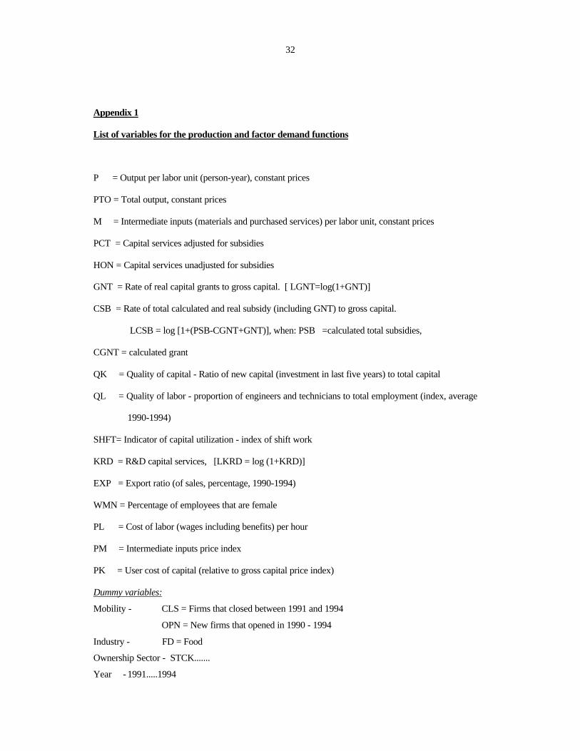
Appendix 1

List of variables for the production and factor demand functions

P = Output per labor unit (person-year), constant prices

PTO = Total output, constant prices

M = Intermediate inputs (materials and purchased services) per labor unit, constant prices

PCT = Capital services adjusted for subsidies

HON = Capital services unadjusted for subsidies

GNT = Rate of real capital grants to gross capital. [ LGNT=log(1+GNT)]

CSB = Rate of total calculated and real subsidy (including GNT) to gross capital.

LCSB = log [1+(PSB-CGNT+GNT)], when: PSB =calculated total subsidies,

CGNT = calculated grant

QK = Quality of capital - Ratio of new capital (investment in last five years) to total capital

QL = Quality of labor - proportion of engineers and technicians to total employment (index, average

1990-1994)

SHFT= Indicator of capital utilization - index of shift work

KRD = R&D capital services, [LKRD = log (1+KRD)]

EXP = Export ratio (of sales, percentage, 1990-1994)

WMN = Percentage of employees that are female

PL = Cost of labor (wages including benefits) per hour

PM = Intermediate inputs price index

PK = User cost of capital (relative to gross capital price index)

Dummy variables:

Mobility - CLS = Firms that closed between 1991 and 1994

OPN = New firms that opened in 1990 - 1994

Industry - FD = Food �

Ownership Sector - STCK.......

Year - 1991.....1994

33

Appendix 2: Production Functions, 1990-1994 (Translog)Dependent Variable: Production – LP

I II III IV

Coef. T. Coef. T. Coef. T. Coef. T.

Intermediate inputs LM .197 6.1 .181 5.6 .215 6.8 .180 5.6

Labor LL .628 21.1 .621 21.3 .612 21.2 .625 21.4

Capital services LPCT .182 9.7 .181 9.7

Capital input LHON .138 7.5 .157 8.7

(LL)2 .131 10.9 .132 11.6 .134 11.6 .132 11.6

(LM)2 .140 18.5 .150 19.5 .141 18.8 .150 19.5

(LHON)2 / (LPCT)2 .005 1.6 .016 4.2 .016 4.4 .016 4.2

LL*LM -.117 -16.5 -.118 -16.8 -.117 -16.6 -.119 -16.9

LL*LHON / LL*LPCT -.000 -.1 .002 .4 -.001 -.3 .002 .4

LM*LHON / LM*LPCT -.015 -3.6 -.028 -6.3 -.023 -5.2 -.028 -6.2

Capital Subsidy LCSB -.257 -6.4 -.115 -3.1

Grants LGNT -.191 -4.2 -.139 -3.1

Quality of capital LQK .019 2.9 .025 3.8 .024 3.7 .022 3.4

Quality of labor LQL .158 3.0 .132 2.6 .118 2.4 .134 2.7

Women ratio WMN -.001 -2.8 -.001 -2.6 -.001 -2.5 -.001 -2.6

Capital Utilization SHFT .002 6.4 .002 5.8 .002 5.5 .002 5.8

R&D capital services LKRD .082 5.7 .113 10.1 .112 10.1 .112 10.1

Mobility (ref.= stayers)

Closed 1991 - 1994 CLS -.088 -3.1 -.111 -4.1 -.113 -4.2 -.111 -4.1

Opened 1990 - 1994 OPN -.052 -3.8 -.049 -3.6 -.051 -3.8 -.048 -3.6

Branch (ref. =electr.) Food FD -.121 -7.7 -.118 -7.9 -.118 -7.9 -.119 -7.9

Textiles TX -.117 -7.0 -.114 -7.0 -.117 -7.9 -.115 -7.1

Printing, paper PA -.028 -1.7 -.021 -1.3 -.020 -7.9 -.021 -1.3

Wood, minerals LH -.054 -3.4 -.053 -3.5 -.054 -7.9 -.054 -3.6

Chemicals, plastic HM -.002 -.1 .006 .4 .002 -7.9 .006 .5

Metals, machinery MA -.010 -.7 .003 .2 .003 -7.9 .003 .2

Sector (ref. = private) Reg. stock market STCK .036 3.0 .030 2.5 .032 2.6 .032 2.7

Histadrut HIST .047 3.6 .052 3.8 .050 3.7 .053 3.9

Kibbutz KIBZ .152 11.1 .139 11.2 .138 10.9 .142 11.2

Public sector PUBL .060 2.1 .034 1.3 .031 1.3 .033 1.3

Year dummies (ref.= 1990) Year 1991 .012 1.1 .012 1.1 .012 1.1 .012 1.1

Year 1992 .012 1.1 .011 1.0 .011 1.0 .011 1.0

Year 1993 -.005 -.5 -.005 -.4 -.006 -.5 -.005 -.4

Year 1994 -.023 -2.0 -.025 -2.2 -.026 -2.3 -.024 -2.2

Intercept 2.357 29.2 2.338 29.4 2.273 28.7 2.335 29.3

R2 .987 .988 .988 .988

Root MSE .185 .186 .186 .186

Mean Elastisities EL 0.23 0.23 0.23 0.23

EK 0.06 0.06 0.06 0.06

EM 0.75 0.75 0.74 0.75

Documents

The Effects of Capital Subsidization on Israeli Industry