Welfare Effects of Unconditonal Cash Transfers:Pre-Analysis Plan∗

Johannes Haushofer†, Jeremy Shapiro‡

June 27, 2013

Abstract

This document describes the analysis plan for the randomized controlled trial (RCT)evaluating the Unconditional Cash Transfer (UCT) of GiveDirectly, Inc. Between June2011 and January 2013, GiveDirectly distributed unconditional cash transfers to 500randomly selected poor rural households in Western Kenya. The transfers were sentto recipients’ mobile phones using the M-Pesa technology. The present RCT includesthree treatments: First, the transfers were randomly chosen to be sent to either theprimary female or the primary male member of the household. Second, the transferswere randomly assigned to be sent as either a large lump-sum payment, or a series ofnine monthly installments of the same total amount. Third, the magnitude of the totaltransfer to each treatment household was randomly chosen to be either $300 or $1,100.The present document outlines the outcome variables and econometric methods we willuse to assess the effect of the program on consumption, food security, assests, incomeand enterprise activity, intrahousehold bargaining, domestic violence, education, health,and preferences, as well as psychological well-being and neurobiological measures ofstress.

JEL Codes: C93, D13, I15, I25, O12Keywords: unconditional cash transfers, randomized controlled trial, impact evalu-

ation.

∗We thank Marie Collins, Faizan Diwan, Chaning Jang, Bena Mwongeli, Joseph Njoroge, KennethOkumu, James Vancel, and Matthew White for excellent research assistance, the team of GiveDirectly (PialiMukhopadhyay, Paul Niehaus, Raphael Gitau) for collaboration, and Petra Persson for designing the intra-household bargaining and domestic violence module. We are grateful for comments to Arun Chandrasekhar,Simon Galle, Ben Golub, Anna Folke Larsen, and Emma Rothschild. This research was supported by CogitoFoundation Grant R-116/10 and NIH Grant R01AG039297 to Johannes Haushofer.†Abdul Latif Jameel Poverty Action Lab, MIT, E53-379, 30 Wadsworth St., Cambridge, MA 02142.

joha@mit.edu‡McKinsey & Co., San Francisco, CA. jeremyshapiro@gmail.com

1

1 Introduction

Cash transfers are a simple intervention to improve the lives of the poor, and have attractedincreased attention both from researchers and policy-makers (Angelucci and De Giorgi 2009;Cunha 2010; Bertrand et al. 2003; Ardington et al. 2009; Posel et al. 2006; Mel et al. 2008;Maluccio and Flores 2005; Attanasio and Mesnard 2006; Gertler et al. 2012; Duflo 2003;Sadoulet et al. 2001; Blattman et al. 2013). However, existing research is still lacking onseveral practical and theoretical questions that are crucial for understanding the impact ofcash transfers. First, should money be given all at once or in many smaller installments?Theory suggests that this depends on recipients’ ability to exercise self-control and on theirinvestment options. Second, should money be given to the husband or wife? This maynot only affect how the money is spent, but also the intra-household distribution of power.Third, should policy-makers give small transfers to many recipients or larger transfers to afew? The Unconditional Cash Transfers (UCT) Project in Rarieda, Western Kenya, aimedto narrow these gaps by providing evidence on the effects of three key design parameters –transfer frequency, recipient gender, and transfer size – on the impacts of a UCT programin rural Kenya.

As CTs can affect a broad range of outcomes, we measure impacts on a wide and innova-tive range of dimensions. First, we document consumption, food security, school enrollment,the physical devleopment of children, entrepreneurial activities, assets and loans, transfersbetween households, fertility and contraception use, and health. Second, we measure stressand mental health through psychological questionnaires, and employ a relatively novel neu-robiological measure of stress (cortisol), measured through saliva. Third, we collect detailedinformation on spousal controlling behavior, intra-household bargaining, and domestic vio-lence. And finally, we consider the impact of UCTs not only on the recipients, but also onthe community. We examine spillovers and general equilibrium effects by measuring effectson non-treated households both in treatment and pure control villages, and the effect onprices, wages, locally available varieties, transportation, and local industrial organization.Understanding such effects is crucial for assessing the feasibility of UCTs as a social pro-tection strategy, yet existing evidence is scarce (Angelucci and De Giorgi 2009). We use adual-level stratified randomized design that allows us to rigorously identify spillover effectsboth within and across villages.

By filling critical gaps in our knowledge of UCTs, we hope that this study will helpto provide both academics and policy-makers with a better understanding of the effect ofunconditional cash transfers on welfare, and the channels through which these effects operate.

2

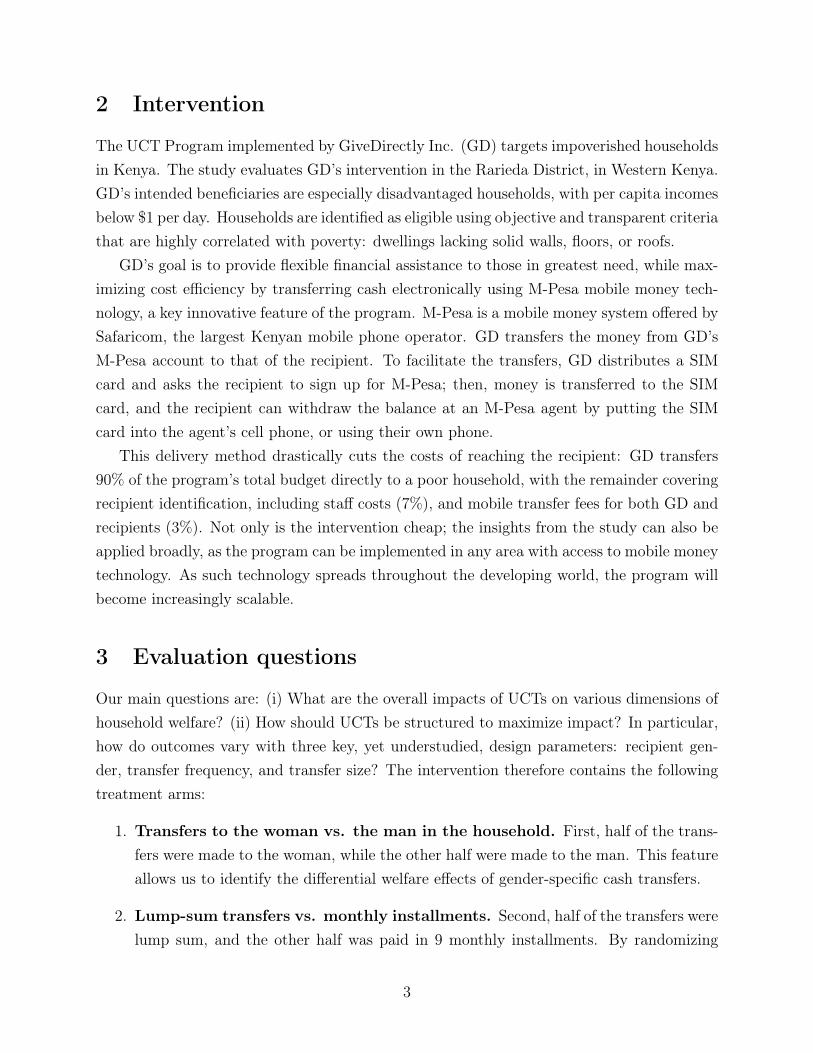
2 Intervention

The UCT Program implemented by GiveDirectly Inc. (GD) targets impoverished householdsin Kenya. The study evaluates GD’s intervention in the Rarieda District, in Western Kenya.GD’s intended beneficiaries are especially disadvantaged households, with per capita incomesbelow $1 per day. Households are identified as eligible using objective and transparent criteriathat are highly correlated with poverty: dwellings lacking solid walls, floors, or roofs.

GD’s goal is to provide flexible financial assistance to those in greatest need, while max-imizing cost efficiency by transferring cash electronically using M-Pesa mobile money tech-nology, a key innovative feature of the program. M-Pesa is a mobile money system offered bySafaricom, the largest Kenyan mobile phone operator. GD transfers the money from GD’sM-Pesa account to that of the recipient. To facilitate the transfers, GD distributes a SIMcard and asks the recipient to sign up for M-Pesa; then, money is transferred to the SIMcard, and the recipient can withdraw the balance at an M-Pesa agent by putting the SIMcard into the agent’s cell phone, or using their own phone.

This delivery method drastically cuts the costs of reaching the recipient: GD transfers90% of the program’s total budget directly to a poor household, with the remainder coveringrecipient identification, including staff costs (7%), and mobile transfer fees for both GD andrecipients (3%). Not only is the intervention cheap; the insights from the study can also beapplied broadly, as the program can be implemented in any area with access to mobile moneytechnology. As such technology spreads throughout the developing world, the program willbecome increasingly scalable.

3 Evaluation questions

Our main questions are: (i) What are the overall impacts of UCTs on various dimensions ofhousehold welfare? (ii) How should UCTs be structured to maximize impact? In particular,how do outcomes vary with three key, yet understudied, design parameters: recipient gen-der, transfer frequency, and transfer size? The intervention therefore contains the followingtreatment arms:

1. Transfers to the woman vs. the man in the household. First, half of the trans-fers were made to the woman, while the other half were made to the man. This featureallows us to identify the differential welfare effects of gender-specific cash transfers.

2. Lump-sum transfers vs. monthly installments. Second, half of the transfers werelump sum, and the other half was paid in 9 monthly installments. By randomizing

3

the month in which the lump sum transfer was made, we kept the discounted presentvalue of the lump-sum and installment transfers similar across the overall lump sumand monthly installment groups.

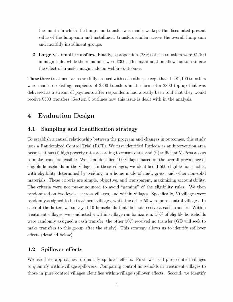
3. Large vs. small transfers. Finally, a proportion (28%) of the transfers were $1,100in magnitude, while the remainder were $300. This manipulation allows us to estimatethe effect of transfer magnitude on welfare outcomes.

These three treatment arms are fully crossed with each other, except that the $1,100 transferswere made to existing recipients of $300 transfers in the form of a $800 top-up that wasdelivered as a stream of payments after respondents had already been told that they wouldreceive $300 transfers. Section 5 outlines how this issue is dealt with in the analysis.

4 Evaluation Design

4.1 Sampling and Identification strategy

To establish a causal relationship between the program and changes in outcomes, this studyuses a Randomized Control Trial (RCT). We first identified Rarieda as an intervention areabecause it has (i) high poverty rates according to census data, and (ii) sufficient M-Pesa accessto make transfers feasible. We then identified 100 villages based on the overall prevalence ofeligible households in the village. In these villages, we identified 1,500 eligible households,with eligibility determined by residing in a home made of mud, grass, and other non-solidmaterials. These criteria are simple, objective, and transparent, maximizing accountability.The criteria were not pre-announced to avoid “gaming” of the eligibility rules. We thenrandomized on two levels – across villages, and within villages. Specifically, 50 villages wererandomly assigned to be treatment villages, while the other 50 were pure control villages. Ineach of the latter, we surveyed 10 households that did not receive a cash transfer. Withintreatment villages, we conducted a within-village randomization: 50% of eligible householdswere randomly assigned a cash transfer; the other 50% received no transfer (GD will seek tomake transfers to this group after the study). This strategy allows us to identify spillovereffects (detailed below).

4.2 Spillover effects

We use three approaches to quantify spillover effects. First, we used pure control villagesto quantify within-village spillovers. Comparing control households in treatment villages tothose in pure control villages identifies within-village spillover effects. Second, we identify

4

spillover effects across villages. Note that these effects could potentially be even more pro-nounced than within villages, if, for instance, entire villages are affected by weather shocks(Rosenzweig and Stark 1989). Using GPS data on village location, we can identify cross-village spillovers, under the assumption that these spillovers are geographically correlated.Third, a separate village-level survey elicited general equilibrium effects of the interventionat the level of the local economy; we surveyed residents of the village on prices, labor supply,wages, crime, investment, community relations (e.g. perceived fairness of targeting criteria)and power dynamics.

4.3 Data collection methods and instruments

Data was collected at baseline and one year after the intervention. A midline with a subsetof questions was administered to a sample of respondents each month after the intervention.Trained interviewers visited the households; both the primary male and the primary female ofthe household were interviewed (separately). Surveys were administered on Netbooks usingthe Blaise survey software. Following standard IPA procedure, we performed backchecksconsisting of 10% of the survey, with a focus on non-changing information, on 10% of allinterviews. This procedure was known to field officers ex ante. Saliva samples were collectedusing the Salivette (Sarstedt, Germany), which has been used extensively in psychologicaland medical research (Kirschbaum and Hellhammer 1989), and more recently in randomizedtrials in developing countries similar to this one (Fernald and Gunnar 2009). It requires therespondent to chew on a sterile cellulose swab, which is then centrifuged and analyzed forsalivary cortisol.

4.4 Power calculation

The sample size of 500 individuals in each of the treatment, control, and pure control con-ditions was chosen based on a power calculation, which showed that a sample of 1,000individuals is sufficient to detect effect sizes of 0.2 SD for all treatment vs. pure controlhouseholds with 89% power. Different treatment arms within the treatment groups (malevs. female recipient, lump-sum vs. monthly, large vs. small transfers) can be compared with60% power.

4.5 Risk and treatment of attrition

Attrition was not a significant concern in this study because it became evident early on inGD’s work in Kenya that respondents were highly interested in maintaining relations with

5

GiveDirectly in the hope of receiving future transfers (although these are never promised).Nevertheless, we used five approaches to control attrition. First, the survey contained adetailed tracking module developed by Innovations for Poverty Action (IPA), the NGO im-plementing the fieldwork. IPA and GD collaborated closely throughout the study to facilitatetracking. Second, we incentivized survey completion through a small appreciation gift (a jarof cooking fat); in addition, respondents earned money from the economic games in the sur-vey. Third, in our power calculations, an attrition rate of 20% would still result in a power of80%. In fact, we only observed 3% attrition between the two visits of the baseline. Finally,we control for attrition econometrically in the analysis, as detailed below.

5 Econometric specifications

5.1 Basic specifications

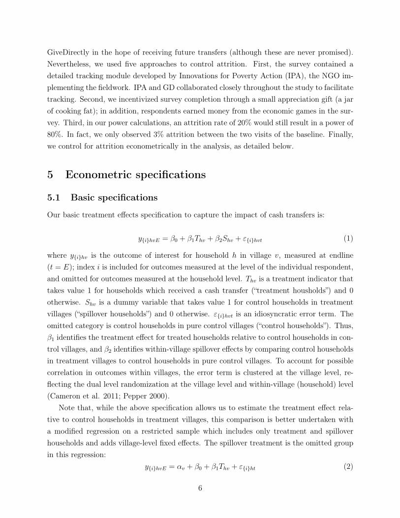
Our basic treatment effects specification to capture the impact of cash transfers is:

y{i}hvE = β0 + β1Thv + β2Shv + ε{i}hvt (1)

where y{i}hv is the outcome of interest for household h in village v, measured at endline(t = E); index i is included for outcomes measured at the level of the individual respondent,and omitted for outcomes measured at the household level. Thv is a treatment indicator thattakes value 1 for households which received a cash transfer (“treatment housholds”) and 0otherwise. Shv is a dummy variable that takes value 1 for control households in treatmentvillages (“spillover households”) and 0 otherwise. ε{i}hvt is an idiosyncratic error term. Theomitted category is control households in pure control villages (“control households”). Thus,β1 identifies the treatment effect for treated households relative to control households in con-trol villages, and β2 identifies within-village spillover effects by comparing control householdsin treatment villages to control households in pure control villages. To account for possiblecorrelation in outcomes within villages, the error term is clustered at the village level, re-flecting the dual level randomization at the village level and within-village (household) level(Cameron et al. 2011; Pepper 2000).

Note that, while the above specification allows us to estimate the treatment effect rela-tive to control households in treatment villages, this comparison is better undertaken witha modified regression on a restricted sample which includes only treatment and spilloverhouseholds and adds village-level fixed effects. The spillover treatment is the omitted groupin this regression:

y{i}hvE = αv + β0 + β1Thv + ε{i}ht (2)

6

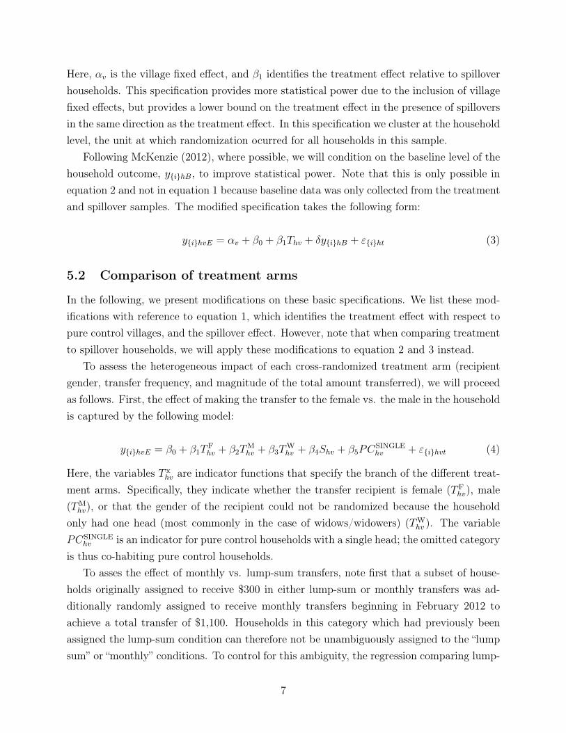
Here, αv is the village fixed effect, and β1 identifies the treatment effect relative to spilloverhouseholds. This specification provides more statistical power due to the inclusion of villagefixed effects, but provides a lower bound on the treatment effect in the presence of spilloversin the same direction as the treatment effect. In this specification we cluster at the householdlevel, the unit at which randomization ocurred for all households in this sample.

Following McKenzie (2012), where possible, we will condition on the baseline level of thehousehold outcome, y{i}hB, to improve statistical power. Note that this is only possible inequation 2 and not in equation 1 because baseline data was only collected from the treatmentand spillover samples. The modified specification takes the following form:

y{i}hvE = αv + β0 + β1Thv + δy{i}hB + ε{i}ht (3)

5.2 Comparison of treatment arms

In the following, we present modifications on these basic specifications. We list these mod-ifications with reference to equation 1, which identifies the treatment effect with respect topure control villages, and the spillover effect. However, note that when comparing treatmentto spillover households, we will apply these modifications to equation 2 and 3 instead.

To assess the heterogeneous impact of each cross-randomized treatment arm (recipientgender, transfer frequency, and magnitude of the total amount transferred), we will proceedas follows. First, the effect of making the transfer to the female vs. the male in the householdis captured by the following model:

y{i}hvE = β0 + β1TFhv + β2T

Mhv + β3T

Whv + β4Shv + β5PC

SINGLEhv + ε{i}hvt (4)

Here, the variables T xhv are indicator functions that specify the branch of the different treat-

ment arms. Specifically, they indicate whether the transfer recipient is female (TFhv), male

(TMhv), or that the gender of the recipient could not be randomized because the household

only had one head (most commonly in the case of widows/widowers) (TWhv ). The variable

PCSINGLEhv is an indicator for pure control households with a single head; the omitted category

is thus co-habiting pure control households.To asses the effect of monthly vs. lump-sum transfers, note first that a subset of house-

holds originally assigned to receive $300 in either lump-sum or monthly transfers was ad-ditionally randomly assigned to receive monthly transfers beginning in February 2012 toachieve a total transfer of $1,100. Households in this category which had previously beenassigned the lump-sum condition can therefore not be unambiguously assigned to the “lumpsum” or “monthly” conditions. To control for this ambiguity, the regression comparing lump-

7

sum and monthly transfers will compare only the groups which did not receive the $1,100transfers, as follows:

y{i}hvE = β0 + β1TMTHhv × T S

hv + β2TLShv × T S

hv + β3TLhv + β4Shv + ε{i}hvt (5)

In this specification, TMTHhv and T LS

hv are indicator variables for having originally been assignedto receiving monthly or lump-sum transfers, respectively, and T S

hv and T Lhv are indicators for

later being randomly assigned to receive the smaller vs. the larger of the two transferamounts, respectively. Note that the group that was originally assigned to the lum-sumcondition and was then additionally assigned to the “large” treatment began to receive astream of transfers after February 2012, and was thus no longer unambiguouly lump-sumafter this time.

Finally, to assess the effect of receiving large compared to small transfers, we will use thefollowing specification:

y{i}hvE = β0 + β1TLhv + β2T

Shv + β3Shv + ε{i}hvt (6)

We will also estimate analogs of the models above which incorporate the relevant interactionterms of the treatment arms, and assess the differential effects of the treatment arms usingthe sample and control variables specified in 2 and 3.

5.3 Comparison of recipient vs. spouse within households

To assess whether cash transfers have differential impacts on the recipient compared totheir spouse within the household, we will allow the impact of the transfer to vary betweenthe individual in the household who receives the transfer and the spouse. The relevantspecification takes the following form:

yihvE = β0 + β1TSELFhv + β2T

SPOUSEhv + β3T

SINGLEhv + β4S

SINGLEhv + β5S

COUPLEhv

+ β6PCSINGLEhv + εihvt

(7)

In this specification, T SELFhv is an indicator variable which takes value 1 for respondents who

live with a spouse and received the transfer themselves, and 0 otherwise; T SPOUSEhv indicates

the respondent’s spouse received a transfer; and T SINGLEhv is an indicator for an individual

who received a transfer and does not live with a spouse. For the spillover, Shv, and purecontrol, PChv, the dummy variables SSINGLE

hv and PCCOUPLEhv indicate whether the respondent

resides without or with a spouse, respectively. The omitted category is PCCOUPLEhv . Thus,

in this model, β1 and β2 identify the treatment effect for respondents who live with their

8

spouse when they receive the transfer and when the spouse receives the transfer, respectively,and β3− β6 identifies the treatment effect for unmarried respondents who receive a transfer.Finally, as before, we will additionally estimate the equation above using the sample andcontrol variables specified in 2 and 3.

5.4 Heterogeneous effects

We will test whether the impact of the cash transfers varies with pre-determined householdand individual characteristics, measured at baseline and denoted by X, which may be eithera household or individual level characteristic. Note that the pure control group was notincluded in the baseline; we will therefore estimate, for household-level outcomes:

y{i}hvE = αv + β0 + β1Thv + β2X{i}hv + β3Thv ×X{i}hv + δy{i}hB + ε{i}hvt (8)

As before, standard errors in this type of specification will be clustered at the householdlevel.

The following model incorporates heterogeneous effects in the equation distinguishingbetween recipient and non-recipient effects:

y{i}hvE = αv + β0 + β1TSELFhv + β2T

SPOUSEhv + β3T

SINGLEhv + β4S

SINGLEhv

+ β5TSELFhv ×X{i}hv + β6T

SPOUSEhv ×X{i}hv + β7T

SINGLEhv ×X{i}hv

+ β8SSINGLEhv ×X{i}hv + β9X{i}hv + δy{i}hB + ε{i}hvt

(9)

We will also estimate analogs of these specifications which incorporate the main effectsand all interaction terms of additional treatment arms (gender or recipient, frequency oftransfer, and aggregate size of the transfer).

This analysis will take the form:

y{i}hvE = αv + β0 + β1TFhv + β2T

Mhv + β3T

Whv + β4T

Fhv ×X{i}hv + β5T

Mhv ×X{i}hv

+ β6TWhv ×X{i}hv + β8X{i}hv + β9S

SINGLEhv + δy{i}hB + ε{i}hvt

(10)

y{i}hvE = αv + β0 + β1TMTHhv + β2T

LShv + β3T

MTHhv ×X{i}hv + β4T

LShv ×X{i}hv

+ β5X{i}hv + δy{i}hB + ε{i}hvt(11)

y{i}hvE = αv + β0 + β1TLhv + β2T

Shv + β3T

Lhv ×X{i}hv + β4T

Shv ×X{i}hv

+ β5X{i}hv + δy{i}hB + ε{i}hvt(12)

Individual outcomes may be tested for heterogeneous impacts both in terms of variables

9

which vary at the household level, Xhv, as well as those that vary at the individual level,Xihv . In cases where the outcome variable is at the household level and heterogeneity isat the individual level, the value of the individual-level variable for the transfer recipient(rather than their spouse) as the source of heterogeneity.

Dimensions of heterogeneous effectsHeterogeneous effects will be considered along the following dimensions:

1. Respondent gender

2. Household type (single vs. joint control)

3. Baseline consumption, asset levels, and land holdings

4. Baseline food security

5. Education level of primary household members

6. Ownership of non-agricultural enterprise at baseline

7. Risk and time preference and decreasing impatience

8. Psychological welfare

9. Domestic violence and bargaining power

5.5 Temporal dynamics of the treatment effect

Both in the lump-sum and monthly conditions, households received transfers at differentpoints in time; the transfers were spread out over the period June 2011 – January 2013.This temporal heterogeneity creates an opportunity to assess the temporal dynamics of thetreatment effect. We achieve this in two ways.

First, we perform a median split on the treatment group according to either the half-waydate between each recipient’s first and last transfer from GD, or the last transfer receivedfrom GD, and define indicator variables TEARLY

{i}hv and T LATE{i}hv for households which received

transfers early vs. late in the study, respectively. We then estimate the following model:

y{i}hvE = β0 + β2TEARLYhv + β3T

LATEhv + β4Shv + ε{i}hvt (13)

The difference between coefficients β2 and β3 is indicative of changing effects of transfersover time. To assess whether the temporal dynamics of the treatment effect are affected byindividual treatment arms, we estimate the following models:

10

y{i}hvE =β0 + β1TFhv × TEARLY

hv + β2TMhv × TEARLY

hv + β3TWhv × TEARLY

hv

+ β4TFhv × T LATE

hv + β5TMhv × T LATE

hv + β6TWhv × T LATE

hv

+ β4Shv + ε{i}hvt

(14)

y{i}hvE =β0 + β1TMTHhv × T S

hv × TEARLYhv + β2T

LShv × T S

hv × TEARLYhv + β3T

Lhv × TEARLY

hv

+ β4TMTHhv × T S

hv × T LATEhv + β5T

LShv × T S

hv × T LATEhv + β6T

Lhv × T LATE

hv

+ β7Shv + ε{i}hvt

(15)

y{i}hvE =β0 + β1TLhv × TEARLY

hv + β2TShv × TEARLY

hv

+ β3TLhv × T LATE

hv + β4TShv × T LATE

hv

+ β5Shv + ε{i}hvt

(16)

In addition, we will distinguish the early vs. late effects of transfers as a function of whetherthe respondent or the spouse is the recipient:

yihvE =β0 + β1TSELFhv × TEARLY

hv + β2TSPOUSEhv × TEARLY

hv + β3TSINGLEhv × TEARLY

hv

+ β4TSELFhv × T LATE

hv + β5TSPOUSEhv × T LATE

hv + β6TSINGLEhv × T LATE

hv

+ β7SSINGLEhv + β8S

COUPLEhv + β9PC

SINGLEhv + εihvt

(17)

We will refine the analysis above by creating separate indicators for the transfer havingbeen completed a specific number of month before the endline survey. We condition onthe assignment to monthly or lump sum transfers, and small or large transfers as these arecorrelated with the end date of the transfer. The specification is below, where T x−y takesvalue 1 if the transfer was completed between x and y months prior to the survey.

y{i}hvE =β0 + β2T<1hv + β3T

1-3hv + β4T

4-6hv + β5T

6-12hv + β6T

LShv

+ β7TMTHhv + β8T

Lhv + β9T

Shv + β10Shv + ε{i}hvt

(18)

In addition to the endline survey, we conducted a midline survey between November 2011and May 2012, in which a subset of respondents answered an abridged version of the ques-tionnaire. For outcomes where both endline and midline data is available, we estimate thefollowing model, where 1 (t = M) is an indicator variable specifying data from the midline:

y{i}hvt =αv + β0 + β2Thv1 (t = M) + β3Thv1 (t = E)

+ δ1 (t = E) + ε{i}hvt(19)

11

Similarly to ?? we will break out the treatment indicator according to the months sincethe survey was conducted, while conditioning on treatment arm or restricting to single arms.

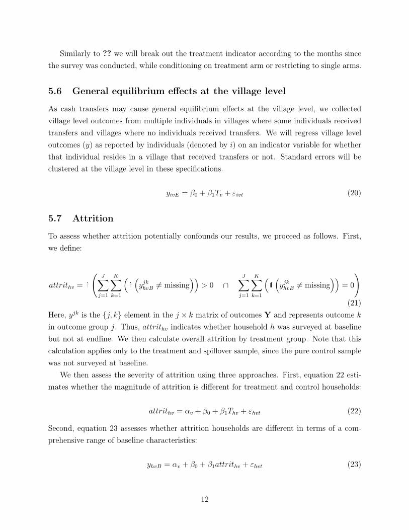
5.6 General equilibrium effects at the village level

As cash transfers may cause general equilibrium effects at the village level, we collectedvillage level outcomes from multiple individuals in villages where some individuals receivedtransfers and villages where no individuals received transfers. We will regress village leveloutcomes (y) as reported by individuals (denoted by i) on an indicator variable for whetherthat individual resides in a village that received transfers or not. Standard errors will beclustered at the village level in these specifications.

yivE = β0 + β1Tv + εivt (20)

5.7 Attrition

To assess whether attrition potentially confounds our results, we proceed as follows. First,we define:

attrithv = 1

(J∑

j=1

K∑k=1

(1

(yjkhvB 6= missing

))> 0 ∩

J∑j=1

K∑k=1

(1

(yjkhvB 6= missing

))= 0

)(21)

Here, yjk is the {j, k} element in the j × k matrix of outcomes Y and represents outcome kin outcome group j. Thus, attrithv indicates whether household h was surveyed at baselinebut not at endline. We then calculate overall attrition by treatment group. Note that thiscalculation applies only to the treatment and spillover sample, since the pure control samplewas not surveyed at baseline.

We then assess the severity of attrition using three approaches. First, equation 22 esti-mates whether the magnitude of attrition is different for treatment and control households:

attrithv = αv + β0 + β1Thv + εhvt (22)

Second, equation 23 assesses whether attrition households are different in terms of a com-prehensive range of baseline characteristics:

yhvB = αv + β0 + β1attrithv + εhvt (23)

12

And third, equation 24 measures whether the baseline characteristics of attrition householdsin the treatment group are significantly different from those in the control group. The samplefor regression will be restricted to attrition households:

(yhvB | attrithv = 1) = β0 + β1Thv + εhvt (24)

We will also estimate analogs of equations 22, 23, and 24 at the individual level, clusteringstandard errors at the village level. If worrying levels of attrition are found, we will adjustfor the potential effect of such attrition using Lee bounds.

5.8 Accounting for multiple inference

As cash transfers are likely to impact a large number of economic behaviors and dimensionsof welfare, and given that our survey instrument often included several questions related toa single behavior or dimension, we will account for multiple hypotheses by using outcomevariable indices and family-wise p-value adjustment.

We have catalogued below the primary groups of outcomes that we intend to considerin the analysis outlined above. For each of these outcome groups, we will construct indices(where possible) and for each of the components of these indices, and will report bothunadjusted p-values as well as p-values corrected for multiple comparisons using the Family-Wise Error Rate.

5.8.1 Construction of indices

To keep the number of outcome variables low and thus allow for greater statistical powereven after adjusting p-values for multiple inference, we will construct indices for several ofour groups of outcome variables. To this end, we will follow the procedure proposed byAnderson (2008), which is reproduced below:

First, for each outcome variable yjk, where j indexes the outcome group and k indexesvariables within outcome groups, we re-code the variable such that high values correspondto positive outcomes.

We then compute the covariance matrix Σj for outcomes in outome group j, whichconsists of elements:

Σjmn =

Njmn∑i=1

yijm − yjmσyjm

yijn − yjnσyjn

(25)

Here, Njmn is the number of non-missing observations for outcomes m and n in outcomegroup j, yjm and yjn are the means for outcomes m and n, respectively, in outcome group j,

13

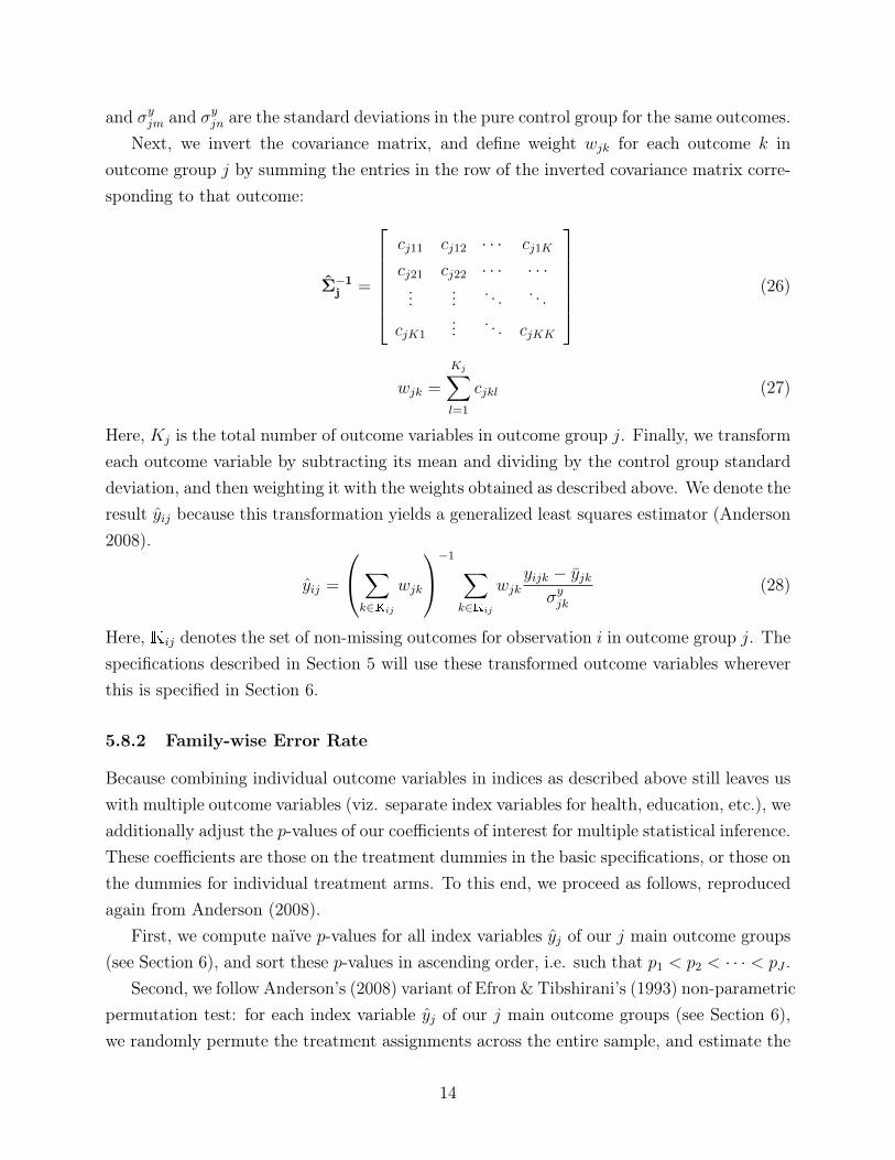
and σyjm and σy

jn are the standard deviations in the pure control group for the same outcomes.Next, we invert the covariance matrix, and define weight wjk for each outcome k in

outcome group j by summing the entries in the row of the inverted covariance matrix corre-sponding to that outcome:

Σ−1j =

cj11 cj12 · · · cj1K

cj21 cj22 · · · · · ·...

... . . . . . .

cjK1... . . . cjKK

(26)

wjk =

Kj∑l=1

cjkl (27)

Here, Kj is the total number of outcome variables in outcome group j. Finally, we transformeach outcome variable by subtracting its mean and dividing by the control group standarddeviation, and then weighting it with the weights obtained as described above. We denote theresult yij because this transformation yields a generalized least squares estimator (Anderson2008).

yij =

∑k∈Kij

wjk

−1 ∑k∈Kij

wjkyijk − yjk

σyjk

(28)

Here, Kij denotes the set of non-missing outcomes for observation i in outcome group j. Thespecifications described in Section 5 will use these transformed outcome variables whereverthis is specified in Section 6.

5.8.2 Family-wise Error Rate

Because combining individual outcome variables in indices as described above still leaves uswith multiple outcome variables (viz. separate index variables for health, education, etc.), weadditionally adjust the p-values of our coefficients of interest for multiple statistical inference.These coefficients are those on the treatment dummies in the basic specifications, or those onthe dummies for individual treatment arms. To this end, we proceed as follows, reproducedagain from Anderson (2008).

First, we compute naïve p-values for all index variables yj of our j main outcome groups(see Section 6), and sort these p-values in ascending order, i.e. such that p1 < p2 < · · · < pJ .

Second, we follow Anderson’s (2008) variant of Efron & Tibshirani’s (1993) non-parametricpermutation test: for each index variable yj of our j main outcome groups (see Section 6),we randomly permute the treatment assignments across the entire sample, and estimate the

14

model of interest to obtain the p-value for the coefficient of interest. We enforce monotonicityin the resulting vector of p-values [p∗1, p

∗2, · · · p∗J ]′ by computing p∗∗r = min{p∗r, p∗r+1, · · · p∗J},

where r is the position of the outcome in the vector of naïve p-values.We then repeat this procedure 10,000 times. The non-parametric p-value, pfwer∗

r , for eachoutcome is the fraction of iterations on which the simulated p-value is smaller than the ob-served p-value. Finally we enforce monotonicity again: pfwer

r = min{pfwer∗r , pfwer∗

r+1 , · · · pfwer∗J }.

This yields the final vector of family-wise error-rate corrected p-values. We will report boththese p-values and the naïve p-values. Within outcome groups, we report naïve p-values forindividual outcome variables other than the indices.

6 Outcome variables

In the following, we list the outcome variables, by outcome group, which we will consider.Variables and outcome groups marked by an asterisk (*) will be excluded when adjusting formultiple testing, either because we have weak a priori hypotheses about them, because theypartly overlap with other variables which are included when adjusting for multiple testing,because they are of lesser interest than other variables, or because the variables are only ofinterest for particular treatment arms (e.g. domestic violence variables when females receivethe transfer).

6.1 Household & Individual

1. Assets

(a) Moveable assets

i. Livestock

A. Cows

B. Small livestock

C. Birds

ii. Furniture

iii. Agricultural tools

iv. Radio or TV

v. Other assets

(b) Savings

(c) Land owned

15

(d) House has non-thatch roof

(e) House has non-mud floor

(f) House has non-mud walls

(g) House has electricity

(h) House has toilet or pit latrine

Index: Total value of moveable assets, savings, and land owned

2. Consumption

(a) Food

i. Food own production

ii. Food bought

iii. Meat & fish

iv. Fruit & vegetables

v. Other food

(b) Temptation good expenditure

(c) Medical expenditure

i. Medical expenditure (respondent)

ii. Medical expenditure (spouse)

iii. Medical expenditure (children)

(d) Education expenditure

(e) Durables expenditure

(f) House expenditure

(g) Social expenditure

(h) Other expenditure

Index: Total expenditure (variables a.-h.)

3. Food security

(a) Meals skipped (adults)

(b) Whole days without food (adults)

16

(c) Meals skipped (children)

(d) Whole days without food (children)

(e) Eat less preferred/cheaper foods

(f) Rely on help from others for food

(g) Purchase food on credit

(h) Hunt, gather wild food, harvest prematurely

(i) Beg because not enough food in the house

(j) All members eat two meals

(k) All members eat until content

(l) Number of times ate meat or fish

(m) Enough food in the house for tomorrow?

(n) Respondent slept hungry

(o) Respendent ate protein

(p) Propotion of HH who ate protein

(q) Proportion of children who ate protein

Food security index (children)*: weighted standardized average of variables c., d.,q.

Food security index (household): weighted standardized average of variables a.-q.

4. Psychological and neurobiological outcomes

(a) Depression (CESD)

(b) Worries

(c) Stress (Cohen)

(d) Happiness (WVS)

(e) Life satisfaction (WVS)

(f) Cortisol

(g) Trust (WVS)

(h) Locus of control (Rotter + WVS)

(i) Optimism (Scheier)

17

(j) Self-esteem (Rosenberg)

Index: weighted standardized average of variables a.-f.

5. Intrahousehold bargaining and domestic violence

(a) Physical violence dummy

(b) Sexual violence dummy

(c) Emotional violence dummy

(d) Justifiability of violence score

(e) Male-focused attitudes score

(f) Male makes decisions dummy

(g) Proportion choosing money for spouse vs. self

Violence index*: weighted standardized average of variables a.-c.

Attitude index*: weighted standardized average of variables d.-e.

Overall intrahousehold index: weighted standardized average of violence and atti-tude indices

6. Health

(a) Medical expenses per episode (entire HH)

(b) Medical expenses per episode (spouses)

(c) Medical expenses per episode (children)

(d) Proportion of household sick/injured

(e) Proportion of children sick/injured

(f) Proportion of sick/injured who could afford treatment

(g) Average number of sick days per HH member

(h) Proportion of illnesses where doctor was consulted

(i) Proportion of newborns vaccinated

(j) Proportion of children < 14 getting checkup

(k) Proportion of children < 5 who died

(l) Children’s anthropometrics index

18

i. BMI

ii. Height for age

iii. Weight for age

iv. Upper-arm circumference

Children’s health index*: weighted standardized average of variables e., i.-l.

Household health index: weighted standardized average of variables d.-f., h.-l.

7. Education

(a) Total education expenditure

(b) Education expenditure per child

(c) Proportion of school-aged children in school

(d) School days missed for economic reasons, per child

(e) Income-generating activities per school-aged child > 6

Index variable: weighted standardized average of variables b.-c.

8. Enterprise variables

(a) Agricultural income (total)

i. Agricultural income (own consumption, total)

A. Agricultural income (own consumption, harvest)

B. Agricultural income (own consumption, animals)

ii. Agricultural income (sales, total)

A. Agricultural income (sales, harvest)

B. Agricultural income (sales, animal products)

C. Agricultural income (sales, animals)

(b) Enterprise profit (6 months)

(c) Enterprise revenue (1 month)

(d) Enterprise revenue (typical month)

(e) New non-agricultural business owner (dummy)

(f) Non-agricultural business owner (dummy)

(g) Number of employees

19

(h) Value of investment in non-agricultural business

Index variable: Agricultural and enterprise income (total)

9. Financial variables*

(a) Value of outstanding loans

(b) Unable to pay loans (12 months)

(c) Value of remittances sent

(d) Value of remittances received

(e) Net remittances

10. Preferences*

(a) Impatience

(b) Decreasing impatience

(c) Risk aversion

(d) Other-regarding preferences

(e) Favors cash transfers from NGOs or government

(f) Random allocation is fair

(g) I am likely to receive the benefit if random allocation is used

11. Temptation goods*: List method

12. Targeting*

6.2 Village-level*

1. Prices

(a) Prices of individual standard items

Index: sum of prices for above list

2. Wages

(a) Likelihood of working for another villager in the same village (spillover vs. purecontrol group only)

20

(b) Average daily wage for working for another villager in the same village (spillovervs. pure control group only)

3. Conflict

(a) Number of conflict episodes in the village in the past year

(b) Multinomial dummy for having less, the same, or more conflict in the villagecompared to a year ago

21

ReferencesAnderson, M. L. (2008). Multiple Inference and Gender Differences in the Effects of

Early Intervention: A Reevaluation of the Abecedarian, Perry Preschool, and EarlyTraining Projects. Journal of the American Statistical Association 103 (484), 1481–1495.

Angelucci, M. and G. De Giorgi (2009). Indirect Effects of an Aid Program: How DoCash Transfers Affect Ineligibles’ Consumption? American Economic Review 99 (1),486–508.

Ardington, C., A. Case, and V. Hosegood (2009). Labor Supply Responses toLarge Social Transfers: Longitudinal Evidence from South Africa. American EconomicJournal: Applied Economics 1 (1), 22–48.

Attanasio, O. and A. Mesnard (2006). The Impact of a Conditional Cash TransferProgramme on Consumption in Colombia. Fiscal Studies 27 (4), 421–442.

Bertrand, M., S. Mullainathan, and D. Miller (2003). Public Policy and Ex-tended Families: Evidence from Pensions in South Africa. World Bank Economic Re-view 17 (1), 27–50.

Blattman, C., N. Fiala, and S. Martinez (2013). Credit Constraints, OccupationalChoice, and the Process of Development: Long Run Evidence from Cash Transfersin Uganda. SSRN Scholarly Paper ID 2268552, Social Science Research Network,Rochester, NY.

Cameron, A. C., J. B. Gelbach, and D. L. Miller (2011). Robust Inference WithMultiway Clustering. Journal of Business & Economic Statistics 29 (2), 238–249.

Cunha, J. (2010). Testing Paternalism: Cash vs. In-kind Transfer in Rural Mexico.Discussion Paper 09-021, Stanford Institute for Economic Policy Research.

Duflo, E. (2003, June). Grandmothers and Granddaughters: Old-Age Pensions andIntrahousehold Allocation in South Africa. The World Bank Economic Review 17 (1),1–25.

Efron, B. and R. Tibshirani (1993). An Introduction to the Bootstrap. Chapman &Hall/CRC.

Fernald, L. C. H. and M. R. Gunnar (2009). Poverty-alleviation program par-ticipation and salivary cortisol in very low-income children. Social Science &Medicine 68 (12), 2180–2189.

Gertler, P. J., S. W. Martinez, and M. Rubio-Codina (2012, January). InvestingCash Transfers to Raise Long-Term Living Standards. American Economic Journal:Applied Economics 4 (1), 164–192.

Kirschbaum, C. and D. H. Hellhammer (1989). Salivary cortisol in psychobiologicalresearch: An overview. Neuropsychobiology 122.

Maluccio, J. A. and R. Flores (2005). Impact evaluation of a conditional cash transferprogram: the Nicaraguan Red de Protección Social. Research reports 141, InternationalFood Policy Research Institute (IFPRI).

22

McKenzie, D. (2012). Beyond baseline and follow-up: The case for more T in experi-ments. Journal of Development Economics 99 (2), 210–221.

Mel, S. d., D. McKenzie, and C. Woodruff (2008). Returns to Capital in Mi-croenterprises: Evidence from a Field Experiment. The Quarterly Journal of Eco-nomics 123 (4), 1329–1372.

Pepper, J. (2000). Robust inferences from random clustered samples: an applicationusing data from the panel study of income dynamics. Economics Letters 75 (3), 341–345.

Posel, D., J. A. Fairburn, and F. Lund (2006). Labour migration and households:A reconsideration of the effects of the social pension on labour supply in South Africa.Economic Modelling 23 (5), 836–853.

Rosenzweig, M. R. and O. Stark (1989). Consumption Smoothing, Migration, andMarriage: Evidence from Rural India. Journal of Political Economy 97 (4), 905–26.

Sadoulet, E., A. d. Janvry, and B. Davis (2001). Cash Transfer Programs withIncome Multipliers: PROCAMPO in Mexico. World Development 29 (6), 1043–1056.

23