Embed Size (px)
Citation preview
164
American Economic Journal: Applied Economics 2012, 4(1): 164–192http://dx.doi.org/10.1257/app.4.1.164
Five years ago when my oldest daughter was in school and we received money from PROGRESA, we saved 600 pesos to buy wood and the other materials for building a chicken coop, and with what was left we bought a few chickens. Since then, we have raised many chickens that we sometimes sell, and we collect 10 to 15 eggs per week that we eat ourselves.
—Oportunidades beneficiary in rural Mexico, August 20041
Cash transfer programs are increasingly common tools for fighting poverty in developing countries. These programs are concerned with providing relief
through income support to those living in extreme poverty, and in the case of condi-tional cash transfer (CCT) programs, with providing incentives for parents to invest in the human capital of children. A major concern for policymakers and develop-ment practitioners has been the extent to which households become dependent on cash transfers to maintain current living standards, and when transitioned off of these programs, whether they will revert to preprogram poverty levels.
1 Quote is from a survey of beneficiaries conducted by the authors in the summer of 2004.
* Gertler: Haas School of Business, University of California, 2220 Piedmont Avenue, Berkeley, CA 94720 (e-mail: [email protected]); Martinez: Inter-American Development Bank, 1300 New York Avenue, NW Washington, DC 20577 (e-mail: [email protected]); Rubio-Codina: The Institute for Fiscal Studies, 7 Ridgmount Street, London WC1E 7AE, UK (e-mail: [email protected]). We have benefited from comments by Orazio Attanasio, Pierre Dubois, Alain de Janvry, Edward Miguel, Elizabeth Sadoulet, John Skinner, Doug Staiger, Chris Udry, two anonymous reviewers, and seminar participants at the University of California-Berkeley, The World Bank, University of Toulouse, Stanford University, Columbia University, Yale University, the Mexican National Institute of Public Health, the NEUDC meetings at Brown University, the ESEM meetings at the University of Vienna, and the LAMES meet-ings at ITAM in Mexico City. We thank the Oportunidades program for its support, and in particular Rogelio Gómez-Hermosillo, Concepción Steta, and Iliana Yaschine. For the qualitative field work associated with this project, we gratefully acknowledge support from UCMEXUS and assistance from Sarit Beith-Halachmi, Giovanna Limongi, Ryo Shiba, and Jennifer Sturdy. The opinions expressed in this document are those of the authors alone.
† To comment on this article in the online discussion forum, or to view additional materials, visit the article page at http://dx.doi.org/10.1257/app.4.1.164.
Investing Cash Transfers to Raise Long-Term Living Standards†
By Paul J. Gertler, Sebastian W. Martinez, and Marta Rubio-Codina*
Using data from a randomized experiment, we find that poor rural Mexican households invested part of their cash transfers from the Oportunidades program in productive assets, increasing agricultural income by almost 10 percent after 18 months of benefits. We esti-mate that for each peso transferred, households consume 74 cents and invest the rest, permanently increasing long-term consumption by about 1.6 cents. Results suggest that cash transfers can achieve long-term increases in consumption through investment in produc-tive activities, thereby permitting beneficiary households to attain higher living standards that are sustained even after transitioning off the program. (JEL D14, H23, I38, O12)
ContentsInvesting Cash Transfers to Raise Long-Term Living Standards† 164
I. The Rural Oportunidades Program 166A. Eligibility and Duration of Benefits 167B. Benefit Structure 167II. Experimental Design and Data 168III. Investment 170A. Dependent Variables 170B. Baseline Balance 171C. Methods 171D. Results 173E. Long-Term Effects 175IV. Agricultural Productivity 176V. Long-Term Living Standards 177A. Methods 178B. Consumption Results 179C. Alternative Income Pathways 179D. Formal and Informal Credit Pathways 180E. Health Pathways 180F. Marginal Propensity to Consume Transfers 181VI. Falsification Tests 182VII. Marginal Propensity to Invest and Long-Run Effects 183A. Empirical Specification 184B. Data and Identification 185C. Results 188VIII. Conclusions 190REFERENCES 191
VOL. 4 NO. 1 165GERtLER Et AL.: INVEStING CASh tRANSFERS
In this paper, we investigate the hypothesis that poor families use some of their cash transfers to invest in productive entrepreneurial activities that raise their liv-ing standards in the long run. There are two primary reasons why cash transfers may lead to increased investments by poor households. First, cash transfers allevi-ate liquidity and credit constraints.2 An infusion of cash through the transfer may help households afford the startup costs associated with entrepreneurial activities (McKenzie and Woodruff 2006). Second, if cash transfers are perceived as a secure and steady source of income over time, risk-adverse households will be more will-ing to invest in riskier but higher return activities. With a secure stream of income from the cash transfer program that is large enough to alleviate liquidity constraints, we would expect to see poor households making more investments in productive assets and activities. If returns on investments are maintained over time, poor house-holds will achieve improvements in long-term living standards that persist even in the absence of the cash transfer program.
We test this hypothesis using data from a controlled randomized experiment of the Oportunidades CCT program in Mexico. We find that beneficiary households increased ownership of productive farm assets, such as farm animals and land for agricultural production, significantly faster than nonbeneficiary households; that agri-cultural production in terms of both crops and animal products increased faster for beneficiary households than nonbeneficiary households; and that this resulted in sig-nificantly higher agricultural income. In fact, we estimate that an 18-month exposure to the program resulted in a 9.6 percent increase in agricultural income. Beneficiary households also started substantially more nonagricultural microenterprises, mainly production of handcrafts for sale, compared to nonbeneficiary households.
We then explore whether returns on these investments persist over time and raise long-term living standards as measured by consumption. We find that even 4 years after households in the control group were incorporated into the program, consump-tion levels for the original treatment households were 5.6 percent higher than for the original control households. This result suggests that returns on investments made by treatment households during the initial 18-month experimental period did in fact translate into improvements in long-term living standards.
Finally, we identify two parameters that require additional assumptions beyond the randomized experimental design. Specifically, we estimate the marginal propen-sity to consume and invest out of transfers and the marginal investment effect, i.e., the impact of one peso transferred on long-term consumption via the investment pathway. We then use these estimated parameters to calculate the effect of the pro-gram on long-term living standards.
Our analysis shows that for each peso transferred, beneficiary households con-sume 74 cents directly and invest the rest. The aggregate effect of the investment yields about a 1.6 cent increase in long-term consumption for each peso of transfers received. Using these estimates to predict the effect of investments on long-term consumption, we estimate that after 5 1/2 years (the period of observation in our data), beneficiary households increase consumption by 41.9 pesos per capita per month.
2 Liquidity constraints and poverty have been explored in Banerjee and Newman (1993); Aghion and Bolton (1997); Lindh and Ohlsson (1998); Lloyd-Ellis and Bernhardt (2000); and Banerjee (2004), amongst others.
166 AMERICAN ECONOMIC JOURNAL: APPLIEd ECONOMICS JANUARy 2012
After 9 years (the minimum expected duration of the program) this amount increases to 53.9 pesos, a substantial amount relative to the 159.8 pesos of baseline per capita consumption for equivalent households that do not participate in the program. As a result, if removed from the program, beneficiary households would most likely not revert to pre-program poverty levels.
To our knowledge, this paper is the first to consider the long-term poverty impli-cations of productive investments made as a result of CCT programs. Our paper is related to a small literature on uses of transfers for nonconsumption purposes. Sadoulet, de Janvry, and Davis (2001) estimate the effect of payments from the Mexican agricultural assistance program, PROCAMPO, on consumption, and find a multiplier greater than 1 consistent with an interpretation of productive invest-ment. Ravallion and Chen (2005) show that the lion’s share of a temporary public cash transfer program in China was saved. Woodruff and Zenteno (2007) and Yang (2008) show that private remittances were used as capital to invest in microenter-prises in Mexico and the Philippines, respectively. Our work also contributes to the literature on the effects of CCT programs on household consumption (Hoddinot and Skoufias 2004; Attanasio and Mesnard 2006; Angelucci and Attanasio 2009). However, these papers do not explore how transfers affect long-term consumption via the investment pathway.
The remainder of the paper is organized as follows. Sections I and II describe the Oportunidades program and its experimental evaluation design and data. In Section III, we show the causal link between cash transfers and investments in productive assets and activities; and in Section IV, we explore the effect of these investments on income and productivity. Section V then tests for sustained long-run effects of the investments on household consumption. Section VI provides a number of falsification tests to validate the impacts observed in Sections III, IV, and V. In Section VII, we move beyond the purely experimental data and estimate the marginal propensity to consume and invest transfers, and the marginal investment effect. Section VIII concludes.
I. The Rural Oportunidades Program3
The Mexican government established the Oportunidades CCT program in 1997. The primary objective was to break the intergenerational transmission of poverty by alleviating current poverty while investing in the human capital of the next gen-eration. To this end, the program provides financial incentives (cash) to parents to invest in the human capital of their children, encouraging investments in health, nutrition, and education. The program is one of the largest CCT interventions in the world, with approximately $4.5 billion US distributed to some 5.8 million benefi-ciary households in 2010 (Oportunidades 2011).
The rural Oportunidades program operates in small credit constrained communi-ties with between 50 to 2,500 inhabitants in isolated and marginalized rural areas.
3 The Oportunidades program was known originally as PROGRESA. The name was changed from PROGRESA to Oportunidades during the Vicente Fox administration in 2000. The data used here are from the rural PROGRESA evaluation. However, we refer to the program under its current name, Oportunidades, throughout the text.
VOL. 4 NO. 1 167GERtLER Et AL.: INVEStING CASh tRANSFERS
Approximately 89 percent of households in these communities engage in farming activities, such as raising crops and farm animals; and 7 percent of households report having a small business or microenterprise. A large number of households are also engaged in the local labor market. Indeed, 65 percent of the households have at least one household member employed in a paid activity, mostly as agricultural day laborers. Credit opportunities are very limited, with only 1.2 percent of communities having a formal credit institution, typically in the form of a credit cooperative (caja de ahorro o cooperativa de crédito). Not surprisingly, only 2.8 percent of house-holds report to have active loans, and from those, almost all are informal loans from friends, neighbors, and relatives.4
A. Eligibility and duration of Benefits
When Oportunidades began rolling out to rural areas in 1997, program eligibility was determined in two stages (Skoufias, Davis, and de la Vega 2001). The program first identified marginalized communities and then identified low-income households within those communities.5 Thus, a household’s eligibility depends on whether it is in an eligible village and on its own poverty level based on a proxy means test. All eligible households living in treatment communities were offered Oportunidades and the vast majority of them (90 percent) enrolled in the program.
Once enrolled, households received benefits for a three-year period conditional on meeting the program requirements. New households were not able to enroll until the next certification period, which prevented migration into treatment communities for Oportunidades benefits. After the initial three-year enrollment period, households in rural areas were “recertified” (reassessed with a proxy means test) to determine future eligibility. If a household was recertified as eligible, it would continue to receive benefits for another three years until the next recertification. If a household was not recertified, then the household was granted six more years of support before being phased off the program. Thus, households could expect a minimum of nine years of benefits upon enrollment.6
B. Benefit Structure
Cash transfers from Oportunidades are given to the female head of the household and are conditional on children attending school, family members obtaining pre-ventive medical care, and attending “pláticas” or education talks on health related
4 Authors’ calculations using data on control households from the Oportunidades household and community questionnaires.
5 Selection criteria for marginalized communities were based on the proportion of households living in very poor conditions, identified by using data from the 1995 census (Conteo de Población y Vivienda). For the selection of eligible households within marginalized communities, Oportunidades conducted a socioeconomic survey of all households, the Encuesta de Características Socioeconómicas de los hogares (ENCASEH). The Government used the ENCASEH to construct a proxy means index and classify households as eligible for treatment (“poor”) or ineligible (“nonpoor”). The original classification scheme designated approximately 52 percent of households as eligible (poor). Subsequently, the government decided that a subset of the nonpoor households had been unduly excluded and expanded the eligibility criteria to include a set of slightly wealthier households in a process called “densification” (Hoddinott and Skoufias 2004).
6 See Oportunidades (2003) for the rules that lay out eligibility and other operational aspects of the program.

168 AMERICAN ECONOMIC JOURNAL: APPLIEd ECONOMICS JANUARy 2012
topics.7 The cash transfers come bimonthly in two forms. The first, received by all beneficiary households, is a fixed cash stipend of 90 pesos per month (in 1997 prices) conditional on family members obtaining preventive medical care, and is intended for families to spend on more and better nutrition.
The second type of transfer comes in the form of educational scholarships and is given conditional on children attending school a minimum of 85 percent of the time and on not repeating a grade more than twice. The educational stipend is provided for each child less than 18 years old who is enrolled in school between the third grade of primary and the third grade (last) of junior high. The educational scholar-ship varies by grade and gender. It rises substantially after graduation from primary school and is higher for girls than boys during junior high school. The rates vary from 60 pesos per month for children enrolled in third grade to 225 pesos per month for females enrolled in the third year of junior high school. Hence, households with more female children enrolled in higher grades are eligible for larger transfers com-pared to similar households with male children enrolled, or children enrolled in lower grades. Beneficiary children also receive money for school supplies once a year during junior high school, and twice a year during primary school.
Only children who were living in the household at the time of incorporation are eligible for the school transfers in order to prevent individual migration into the household. While children fostered into the household at a later date are not eligible for the education transfers, children born into the household will be eligible for future educational transfers once they reach nine years old and enter the third grade of primary school.
Finally, total transfers for any given household are capped at a predetermined upper limit of 550 pesos per month. The cap implies that a household cannot receive an unlimited amount by increasing the number of children enrolled in school. It also implicitly implies that enrolling more than three older children (per household) in school will not increase the amount of transfers received by the household. There appears to have been no effect of the program on fertility rates or family structure (Stecklov et al. 2007).
II. Experimental Design and Data
The identification in this paper relies on experimental variation in program treat-ment, generated through the Oportunidades randomized evaluation. The evaluation sample includes all households in 506 rural communities in 7 states. Communities were randomly assigned to treatment (320 communities) and control (186 commu-nities) groups, which were phased into the program at different points in time as part of the program’s national scale-up.8 Eligible households in treatment communities
7 If a female head of household was not present or able to receive payments, an alternate household member is designated for receipt of payment. Compliance with conditions was verified through the clinics and schools, who certified whether households actually completed the required health care visits, and whether kids attended schools. About 1 percent of households were denied the cash transfer for noncompliance.
8 Given budgetary and logistical constraints, the government could not enroll all eligible families in the coun-try simultaneously and had to phase in enrollment over time. To make implementation feasible, the government decided that whole communities would be enrolled at a time, and that they would be enrolled as fast as possible so that no eligible household would be kept out of the program.
VOL. 4 NO. 1 169GERtLER Et AL.: INVEStING CASh tRANSFERS
began receiving benefits starting in March/April of 1998, while eligible house-holds in control communities were incorporated in November/December of 1999. In order to minimize anticipation effects, households in control communities were not informed that Oportunidades would provide benefits to them until two months before incorporation. Behrman and Todd (1999) confirm that the original random-ization balanced the control and treatment communities; and Attanasio, Meghir, and Santiago (forthcoming) explicitly test, but find no evidence of, anticipation effects amongst control households.
The data used in this paper are primarily from the Oportunidades rural evalua-tion surveys, the Encuesta de Evaluación de los hogares Rurales (ENCEL).9 The ENCEL interviewed all households—eligible and ineligible—living in the 506 eval-uation communities every 6 months between March 1998 and November 2000, and again in November 2003.10 In addition, we use data from the 1997 ENCASEH cen-sus for baseline (pre-intervention) information and administrative records on trans-fer of payments to households in the evaluation sample. The ENCASEH contains the basic socioeconomic household information that was used to classify house-holds in selected communities as eligible or ineligible for treatment.
For the core of the analysis, we work with the sample of eligible households originally classified as poor.11 We also use ineligible (nonpoor) households for falsification robustness checks. The treatment group includes 7,658 eligi-ble households in treatment communities that were offered to begin the pro-gram in March/April of 1998, and the control group includes 4,644 eligible households in control communities that were offered to begin the program in November/December of 1999.12
Sample attrition for the 6-year panel is relatively low, at 10.32 percent for treat-ment households and 9.86 percent for control households. Because attrition rates are not significantly different for the two groups, we believe that neither attrition nor selective migration is a major concern for our analysis. First, a 10 percent attrition rate over a 6-year period implies an average yearly rate between rounds as low as 1.6 percent. Second, if the program was expected to reduce migration by providing monetary incentives to remain in the community, then we would expect a higher attrition rate in treatment areas than in control areas, whereas in reality the opposite occurred. Finally, statistical tests on the subsample of nonattriter households show that treatment and controls are well balanced in terms of their baseline observables (results available upon request).
9 These data are publicly available at www.oportunidades.gob.mx10 ENCEL follow-up surveys were collected in March 1998, October 1998, May 1999, November 1999, May
2000, and November 2000. We do not use the March 1998 ENCEL survey as it excludes many of the variables of interest.
11 We do not use the “densified” households—i.e., the set of wealthier and older households that were deemed eligible later—because their process of incorporation in the program is less well documented. Moreover, many of these households suffered substantial administrative delays in the receipt of benefits (Hoddinott and Skoufias 2004). Because households were categorized as “densified” in both treatment and control communities, and under the same criteria, excluding them does not compromise the internal consistency of our estimates.
12 We drop 53 households that report a head or a head’s spouse younger than 13 or older than 90. The proportion of households we drop for this reason is balanced between treatment and control groups.
170 AMERICAN ECONOMIC JOURNAL: APPLIEd ECONOMICS JANUARy 2012
III. Investment
The central question explored in this paper is whether poor households invest part of their cash transfers in productive enterprises that lead to improvements in long-term living standards. In this section, we address the first part of this question and estimate the intent-to-treat impact of Oportunidades on investments in productive agricultural assets, such as animals and land, and nonagricultural microenterprises. To this end, we first use the three rounds of data spanning the purely experimental period, i.e., before the randomized control group was incorporated into the program: October 1998, May 1999, and November 1999. In the final subsection, we include data from November 2003, once both treatment and controls are receiving benefits, to test for sustained program impacts over time.
A. dependent Variables
The dependent variables for investment outcomes are constructed from infor-mation on animal ownership at the time of the survey, the amount of land in use over the 12 months preceding the interview, and nonagricultural microenterprise activity over the month before the interview. We define production animals to be those whose meat and/or byproducts (milk, cheese, eggs, etc.) are sold and consumed. These include goats and sheep, cows, poultry (chickens, hens, and tur-keys), pigs, and rabbits. We define draft animals to be those traditionally used for plowing the fields and for transportation purposes. These include donkeys, mules, horses, and oxen.13 We aggregate all animals into the total value of production animals and the total value of draft animals using price data on animal sales avail-able in the October 1998 and May 1999 rounds (deflated to 1997 prices).14 Land is measured in hectares and includes all plots used by the household for agriculture, grazing, and forestry purposes.
We also look at the impact of the program on operating nonagricultural micro-enterprises. The ENCELs ask about household involvement in self-owned nonagri-cultural activities that generated income during the month preceding the interview. We define the indicator “microenterprise” as participation in any of the following activities: sewing clothes; making food for sale; carpentry and construction; sale of nonfood items, such as handcrafts, repair of artifacts, or machinery; or other activi-ties done in the context of self-employment.
13 Table A1 in the online Appendix provides additional details on the construction of the dependent variables and the survey rounds data is available for.
14 We take household reports on animal sales prices and construct the median community sale price per animal type. As we discuss later, Table A2 in the online Appendix shows no differences in average animal prices in treat-ment and control communities during the experimental period. We also checked household reports on prices against data we collected in the summer of 2004. Animal prices and other information collected during our fieldwork are available upon request.
VOL. 4 NO. 1 171GERtLER Et AL.: INVEStING CASh tRANSFERS
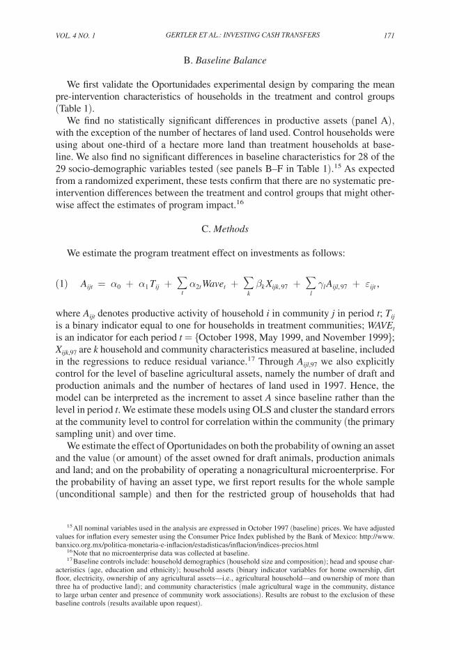
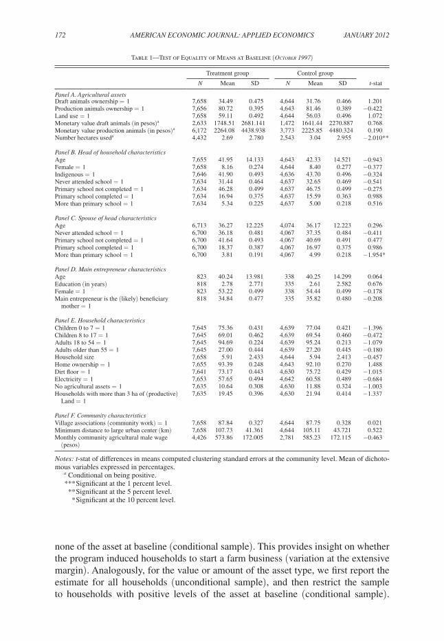
B. Baseline Balance
We first validate the Oportunidades experimental design by comparing the mean pre-intervention characteristics of households in the treatment and control groups (Table 1).
We find no statistically significant differences in productive assets (panel A), with the exception of the number of hectares of land used. Control households were using about one-third of a hectare more land than treatment households at base-line. We also find no significant differences in baseline characteristics for 28 of the 29 socio-demographic variables tested (see panels B–F in Table 1).15 As expected from a randomized experiment, these tests confirm that there are no systematic pre-intervention differences between the treatment and control groups that might other-wise affect the estimates of program impact.16
C. Methods
We estimate the program treatment effect on investments as follows:
(1) A ijt = α 0 + α 1 t ij + ∑ t
α 2t Wav e t + ∑ k
β k X ijk, 97 + ∑ l
γ l A ijl, 97 + ε ijt ,
where Aijt denotes productive activity of household i in community j in period t; tij is a binary indicator equal to one for households in treatment communities; WAVEt is an indicator for each period t = {October 1998, May 1999, and November 1999}; Xijk,97 are k household and community characteristics measured at baseline, included in the regressions to reduce residual variance.17 Through Aijl,97 we also explicitly control for the level of baseline agricultural assets, namely the number of draft and production animals and the number of hectares of land used in 1997. Hence, the model can be interpreted as the increment to asset A since baseline rather than the level in period t. We estimate these models using OLS and cluster the standard errors at the community level to control for correlation within the community (the primary sampling unit) and over time.
We estimate the effect of Oportunidades on both the probability of owning an asset and the value (or amount) of the asset owned for draft animals, production animals and land; and on the probability of operating a nonagricultural microenterprise. For the probability of having an asset type, we first report results for the whole sample (unconditional sample) and then for the restricted group of households that had
15 All nominal variables used in the analysis are expressed in October 1997 (baseline) prices. We have adjusted values for inflation every semester using the Consumer Price Index published by the Bank of Mexico: http://www.banxico.org.mx/politica-monetaria-e-inflacion/estadisticas/inflacion/indices-precios.html
16 Note that no microenterprise data was collected at baseline.17 Baseline controls include: household demographics (household size and composition); head and spouse char-
acteristics (age, education and ethnicity); household assets (binary indicator variables for home ownership, dirt floor, electricity, ownership of any agricultural assets—i.e., agricultural household—and ownership of more than three ha of productive land); and community characteristics (male agricultural wage in the community, distance to large urban center and presence of community work associations). Results are robust to the exclusion of these baseline controls (results available upon request).
172 AMERICAN ECONOMIC JOURNAL: APPLIEd ECONOMICS JANUARy 2012
none of the asset at baseline (conditional sample). This provides insight on whether the program induced households to start a farm business (variation at the extensive margin). Analogously, for the value or amount of the asset type, we first report the estimate for all households (unconditional sample), and then restrict the sample to households with positive levels of the asset at baseline (conditional sample).
Table 1—Test of Equality of Means at Baseline (OctOber 1997)
Treatment group Control group
N Mean SD N Mean SD t-stat
Panel A. Agricultural assetsDraft animals ownership = 1 7,658 34.49 0.475 4,644 31.76 0.466 1.201Production animals ownership = 1 7,656 80.72 0.395 4,643 81.46 0.389 −0.422Land use = 1 7,658 59.11 0.492 4,644 56.03 0.496 1.072Monetary value draft animals (in pesos)a 2,633 1748.51 2681.141 1,472 1641.44 2270.887 0.768Monetary value production animals (in pesos)a 6,172 2264.08 4438.938 3,773 2225.85 4480.324 0.190Number hectares useda 4,432 2.69 2.780 2,543 3.04 2.955 −2.010**
Panel B. head of household characteristicsAge 7,655 41.95 14.133 4,643 42.33 14.521 −0.943Female = 1 7,658 8.16 0.274 4,644 8.40 0.277 −0.377Indigenous = 1 7,646 41.90 0.493 4,636 43.70 0.496 −0.324Never attended school = 1 7,634 31.44 0.464 4,637 32.65 0.469 −0.541Primary school not completed = 1 7,634 46.28 0.499 4,637 46.75 0.499 −0.275Primary school completed = 1 7,634 16.94 0.375 4,637 15.59 0.363 0.988More than primary school = 1 7,634 5.34 0.225 4,637 5.00 0.218 0.516
Panel C. Spouse of head characteristicsAge 6,713 36.27 12.225 4,074 36.17 12.223 0.296Never attended school = 1 6,700 36.18 0.481 4,067 37.35 0.484 −0.411Primary school not completed = 1 6,700 41.64 0.493 4,067 40.69 0.491 0.477Primary school completed = 1 6,700 18.37 0.387 4,067 16.97 0.375 0.986More than primary school = 1 6,700 3.81 0.191 4,067 4.99 0.218 −1.954*
Panel d. Main entrepreneur characteristicsAge 823 40.24 13.981 338 40.25 14.299 0.064Education (in years) 818 2.78 2.771 335 2.61 2.582 0.676Female = 1 823 53.22 0.499 338 54.44 0.499 −0.178Main entrepreneur is the (likely) beneficiary mother = 1
818 34.84 0.477 335 35.82 0.480 −0.208
Panel E. household characteristicsChildren 0 to 7 = 1 7,645 75.36 0.431 4,639 77.04 0.421 −1.396Children 8 to 17 = 1 7,645 69.01 0.462 4,639 69.54 0.460 −0.472Adults 18 to 54 = 1 7,645 94.69 0.224 4,639 95.24 0.213 −1.079Adults older than 55 = 1 7,645 27.00 0.444 4,639 27.20 0.445 −0.180Household size 7,658 5.91 2.433 4,644 5.94 2.413 −0.457Home ownership = 1 7,655 93.39 0.248 4,643 92.10 0.270 1.488Dirt floor = 1 7,641 73.17 0.443 4,630 75.72 0.429 −1.015Electricity = 1 7,653 57.65 0.494 4,642 60.58 0.489 −0.684No agricultural assets = 1 7,635 10.64 0.308 4,630 11.88 0.324 −1.003Households with more than 3 ha of (productive) Land = 1
7,635 19.45 0.396 4,630 21.94 0.414 −1.337
Panel F. Community characteristicsVillage associations (community work) = 1 7,658 87.84 0.327 4,644 87.75 0.328 0.021Minimum distance to large urban center (km) 7,658 107.73 41.361 4,644 105.11 43.721 0.522Monthly community agricultural male wage (pesos)
4,426 573.86 172.005 2,781 585.23 172.115 −0.463
Notes: t-stat of differences in means computed clustering standard errors at the community level. Mean of dichoto-mous variables expressed in percentages.
a Conditional on being positive.*** Significant at the 1 percent level. ** Significant at the 5 percent level. * Significant at the 10 percent level.
VOL. 4 NO. 1 173GERtLER Et AL.: INVEStING CASh tRANSFERS
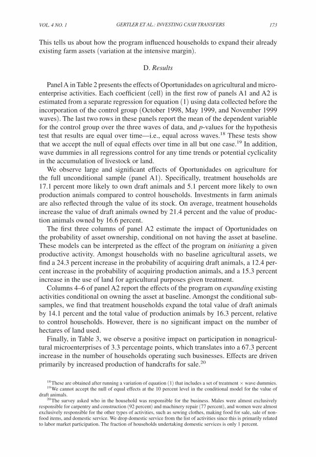
This tells us about how the program influenced households to expand their already existing farm assets (variation at the intensive margin).
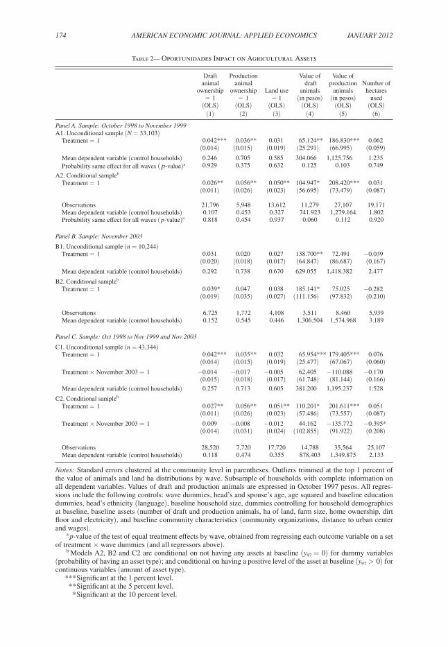
D. Results
Panel A in Table 2 presents the effects of Oportunidades on agricultural and micro-enterprise activities. Each coefficient (cell) in the first row of panels A1 and A2 is estimated from a separate regression for equation (1) using data collected before the incorporation of the control group (October 1998, May 1999, and November 1999 waves). The last two rows in these panels report the mean of the dependent variable for the control group over the three waves of data, and p-values for the hypothesis test that results are equal over time—i.e., equal across waves.18 These tests show that we accept the null of equal effects over time in all but one case.19 In addition, wave dummies in all regressions control for any time trends or potential cyclicality in the accumulation of livestock or land.
We observe large and significant effects of Oportunidades on agriculture for the full unconditional sample (panel A1). Specifically, treatment households are 17.1 percent more likely to own draft animals and 5.1 percent more likely to own production animals compared to control households. Investments in farm animals are also reflected through the value of its stock. On average, treatment households increase the value of draft animals owned by 21.4 percent and the value of produc-tion animals owned by 16.6 percent.
The first three columns of panel A2 estimate the impact of Oportunidades on the probability of asset ownership, conditional on not having the asset at baseline. These models can be interpreted as the effect of the program on initiating a given productive activity. Amongst households with no baseline agricultural assets, we find a 24.3 percent increase in the probability of acquiring draft animals, a 12.4 per-cent increase in the probability of acquiring production animals, and a 15.3 percent increase in the use of land for agricultural purposes given treatment.
Columns 4–6 of panel A2 report the effects of the program on expanding existing activities conditional on owning the asset at baseline. Amongst the conditional sub-samples, we find that treatment households expand the total value of draft animals by 14.1 percent and the total value of production animals by 16.3 percent, relative to control households. However, there is no significant impact on the number of hectares of land used.
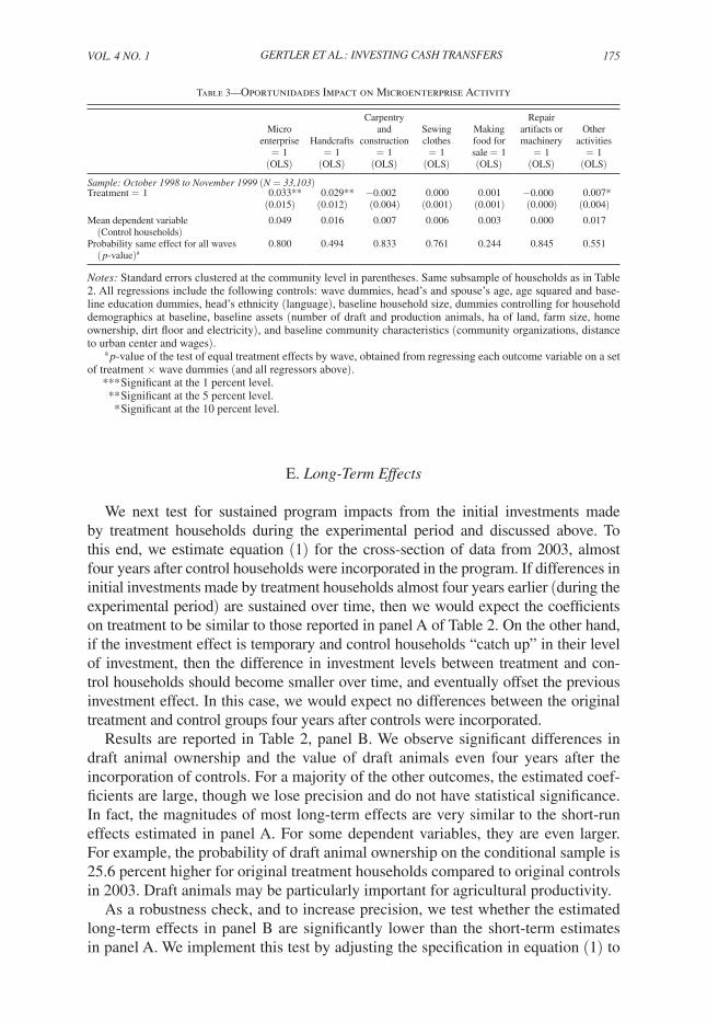
Finally, in Table 3, we observe a positive impact on participation in nonagricul-tural microenterprises of 3.3 percentage points, which translates into a 67.3 percent increase in the number of households operating such businesses. Effects are driven primarily by increased production of handcrafts for sale.20
18 These are obtained after running a variation of equation (1) that includes a set of treatment × wave dummies.19 We cannot accept the null of equal effects at the 10 percent level in the conditional model for the value of
draft animals.20 The survey asked who in the household was responsible for the business. Males were almost exclusively
responsible for carpentry and construction (92 percent) and machinery repair (77 percent), and women were almost exclusively responsible for the other types of activities, such as sewing clothes, making food for sale, sale of non-food items, and domestic service. We drop domestic service from the list of activities since this is primarily related to labor market participation. The fraction of households undertaking domestic services is only 1 percent.
174 AMERICAN ECONOMIC JOURNAL: APPLIEd ECONOMICS JANUARy 2012
Table 2— Oportunidades Impact on Agricultural Assets
Draftanimal
ownership= 1
(OLS)
Production animal
ownership= 1
(OLS)
Land use = 1
(OLS)
Value of draft
animals(in pesos)
(OLS)
Value of production
animals(in pesos)
(OLS)
Number of hectares
used(OLS)
(1) (2) (3) (4) (5) (6)
Panel A. Sample: October 1998 to November 1999A1. Unconditional sample (N = 33,103) Treatment = 1 0.042*** 0.036** 0.031 65.124** 186.830*** 0.062
(0.014) (0.015) (0.019) (25.291) (66.995) (0.059) Mean dependent variable (control households) 0.246 0.705 0.585 304.066 1,125.756 1.235 Probability same effect for all waves ( p-value)a 0.929 0.375 0.632 0.125 0.103 0.749
A2. Conditional sampleb
Treatment = 1 0.026** 0.056** 0.050** 104.947* 208.420*** 0.031 (0.011) (0.026) (0.023) (56.695) (73.479) (0.087)
Observations 21,796 5,948 13,612 11,279 27,107 19,171 Mean dependent variable (control households) 0.107 0.453 0.327 741.923 1,279.164 1.802 Probability same effect for all waves ( p-value)a 0.818 0.454 0.937 0.060 0.112 0.920
Panel B. Sample: November 2003
B1. Unconditional sample (n = 10,244) Treatment = 1 0.031 0.020 0.027 138.700** 72.491 −0.039
(0.020) (0.018) (0.017) (64.847) (86.687) (0.167) Mean dependent variable (control households) 0.292 0.738 0.670 629.055 1,418.382 2.477
B2. Conditional sampleb
Treatment = 1 0.039* 0.047 0.038 185.141* 75.025 −0.282(0.019) (0.035) (0.027) (111.156) (97.832) (0.210)
Observations 6,725 1,772 4,108 3,511 8,460 5,939 Mean dependent variable (control households) 0.152 0.545 0.446 1,306.504 1,574.968 3.189
Panel C. Sample: Oct 1998 to Nov 1999 and Nov 2003
C1. Unconditional sample (n = 43,344) Treatment = 1 0.042*** 0.035** 0.032 65.954*** 179.405*** 0.076
(0.014) (0.015) (0.019) (25.477) (67.067) (0.060) Treatment × November 2003 = 1 −0.014 −0.017 −0.005 62.405 −110.088 −0.170
(0.015) (0.018) (0.017) (61.748) (81.144) (0.166) Mean dependent variable (control households) 0.257 0.713 0.605 381.200 1,195.237 1.528
C2. Conditional sampleb
Treatment = 1 0.027** 0.056** 0.051** 110.201* 201.611*** 0.051(0.011) (0.026) (0.023) (57.486) (73.557) (0.087)
Treatment × November 2003 = 1 0.009 −0.008 −0.012 44.162 −135.772 −0.395*(0.014) (0.031) (0.024) (102.855) (91.922) (0.208)
Observations 28,520 7,720 17,720 14,788 35,564 25,107 Mean dependent variable (control households) 0.118 0.474 0.355 878.403 1,349.875 2.133
Notes: Standard errors clustered at the community level in parentheses. Outliers trimmed at the top 1 percent of the value of animals and land ha distributions by wave. Subsample of households with complete information on all dependent variables. Values of draft and production animals are expressed in October 1997 pesos. All regres-sions include the following controls: wave dummies, head’s and spouse’s age, age squared and baseline education dummies, head’s ethnicity (language), baseline household size, dummies controlling for household demographics at baseline, baseline assets (number of draft and production animals, ha of land, farm size, home ownership, dirt floor and electricity), and baseline community characteristics (community organizations, distance to urban center and wages).
a p-value of the test of equal treatment effects by wave, obtained from regressing each outcome variable on a set of treatment × wave dummies (and all regressors above).
b Models A2, B2 and C2 are conditional on not having any assets at baseline (y97 = 0) for dummy variables (probability of having an asset type); and conditional on having a positive level of the asset at baseline (y97 > 0) for continuous variables (amount of asset type).
*** Significant at the 1 percent level. ** Significant at the 5 percent level. * Significant at the 10 percent level.
VOL. 4 NO. 1 175GERtLER Et AL.: INVEStING CASh tRANSFERS
E. Long-term Effects
We next test for sustained program impacts from the initial investments made by treatment households during the experimental period and discussed above. To this end, we estimate equation (1) for the cross-section of data from 2003, almost four years after control households were incorporated in the program. If differences in initial investments made by treatment households almost four years earlier (during the experimental period) are sustained over time, then we would expect the coefficients on treatment to be similar to those reported in panel A of Table 2. On the other hand, if the investment effect is temporary and control households “catch up” in their level of investment, then the difference in investment levels between treatment and con-trol households should become smaller over time, and eventually offset the previous investment effect. In this case, we would expect no differences between the original treatment and control groups four years after controls were incorporated.
Results are reported in Table 2, panel B. We observe significant differences in draft animal ownership and the value of draft animals even four years after the incorporation of controls. For a majority of the other outcomes, the estimated coef-ficients are large, though we lose precision and do not have statistical significance. In fact, the magnitudes of most long-term effects are very similar to the short-run effects estimated in panel A. For some dependent variables, they are even larger. For example, the probability of draft animal ownership on the conditional sample is 25.6 percent higher for original treatment households compared to original controls in 2003. Draft animals may be particularly important for agricultural productivity.
As a robustness check, and to increase precision, we test whether the estimated long-term effects in panel B are significantly lower than the short-term estimates in panel A. We implement this test by adjusting the specification in equation (1) to
Table 3—Oportunidades Impact on Microenterprise Activity
Micro enterprise
= 1(OLS)
Handcrafts= 1
(OLS)
Carpentry and
construction= 1
(OLS)
Sewing clothes= 1
(OLS)
Makingfood for sale = 1(OLS)
Repair artifacts or machinery
= 1(OLS)
Other activities
= 1(OLS)
Sample: October 1998 to November 1999 (N = 33,103)Treatment = 1 0.033** 0.029** −0.002 0.000 0.001 −0.000 0.007*
(0.015) (0.012) (0.004) (0.001) (0.001) (0.000) (0.004)Mean dependent variable (Control households)
0.049 0.016 0.007 0.006 0.003 0.000 0.017
Probability same effect for all waves ( p-value)a
0.800 0.494 0.833 0.761 0.244 0.845 0.551
Notes: Standard errors clustered at the community level in parentheses. Same subsample of households as in Table 2. All regressions include the following controls: wave dummies, head’s and spouse’s age, age squared and base-line education dummies, head’s ethnicity (language), baseline household size, dummies controlling for household demographics at baseline, baseline assets (number of draft and production animals, ha of land, farm size, home ownership, dirt floor and electricity), and baseline community characteristics (community organizations, distance to urban center and wages).
a p-value of the test of equal treatment effects by wave, obtained from regressing each outcome variable on a set of treatment × wave dummies (and all regressors above).
*** Significant at the 1 percent level. ** Significant at the 5 percent level. * Significant at the 10 percent level.
176 AMERICAN ECONOMIC JOURNAL: APPLIEd ECONOMICS JANUARy 2012
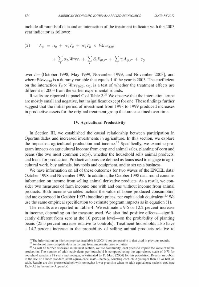
include all rounds of data and an interaction of the treatment indicator with the 2003 year indicator as follows:
(2) A ijt = α 0 + α 1 t ij + α 2 t ij × Wav e 2003
+ ∑ t
α 2t Wav e t + ∑ k
β k X ijk,97 + ∑ l
γ l A ijl,97 + ε ijt
over t = {October 1998, May 1999, November 1999, and November 2003}, and where Wave2003 is a dummy variable that equals 1 if the year is 2003. The coefficient on the interaction tij × Wave2003, α2, is a test of whether the treatment effects are different in 2003 from the earlier experimental rounds.
Results are reported in panel C of Table 2.21 We observe that the interaction terms are mostly small and negative, but insignificant except for one. These findings further suggest that the initial period of investment from 1998 to 1999 produced increases in productive assets for the original treatment group that are sustained over time.
IV. Agricultural Productivity
In Section III, we established the causal relationship between participation in Oportunidades and increased investments in agriculture. In this section, we explore the impact on agricultural production and income.22 Specifically, we examine pro-gram impacts on agricultural income from crop and animal sales, planting of corn and beans (the two most common crops), whether the household sells animal products, and loans for production. Productive loans are defined as loans used to engage in agri-cultural work, buy animals, buy tools and equipment, and to set up a business.
We have information on all of these outcomes for two waves of the ENCEL data: October 1998 and November 1999. In addition, the October 1998 data round contains information on income from selling animal derivative products. As a result, we con-sider two measures of farm income: one with and one without income from animal products. Both income variables include the value of home produced consumption and are expressed in October 1997 (baseline) prices, per capita adult equivalent.23 We use the same empirical specification to estimate program impacts as in equation (1).
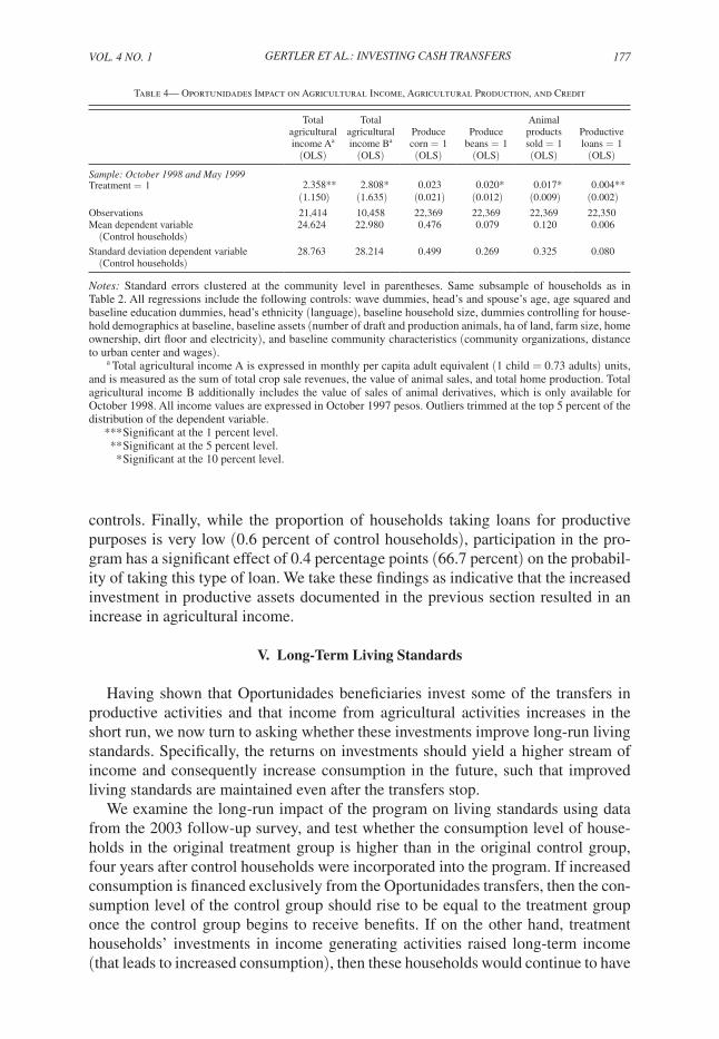
The results are reported in Table 4. We estimate a 9.6 or 12.2 percent increase in income, depending on the measure used. We also find positive effects—signifi-cantly different from zero at the 10 percent level—on the probability of planting beans (25.3 percent increase relative to controls). Treatment households also have a 14.2 percent increase in the probability of selling animal products relative to
21 The information on microenterprises available in 2003 is not comparable to that used in previous rounds.22 We do not have complete data on income from microenterprise activities.23 As will be further discussed in the next section, we use community level prices to impute the value of home
production. The number of adult equivalents per household is computed using the equivalence scale of 0.73 for household members 18 years and younger, as estimated by Di Maro (2004) for this population. Results are robust to the use of a more standard adult equivalence scale—namely, counting each child younger than 12 as half an adult. Results are also preserved albeit with somewhat lower precision when no adult equivalence scale is used (see Table A3 in the online Appendix).
VOL. 4 NO. 1 177GERtLER Et AL.: INVEStING CASh tRANSFERS
controls. Finally, while the proportion of households taking loans for productive purposes is very low (0.6 percent of control households), participation in the pro-gram has a significant effect of 0.4 percentage points (66.7 percent) on the probabil-ity of taking this type of loan. We take these findings as indicative that the increased investment in productive assets documented in the previous section resulted in an increase in agricultural income.
V. Long-Term Living Standards
Having shown that Oportunidades beneficiaries invest some of the transfers in productive activities and that income from agricultural activities increases in the short run, we now turn to asking whether these investments improve long-run living standards. Specifically, the returns on investments should yield a higher stream of income and consequently increase consumption in the future, such that improved living standards are maintained even after the transfers stop.
We examine the long-run impact of the program on living standards using data from the 2003 follow-up survey, and test whether the consumption level of house-holds in the original treatment group is higher than in the original control group, four years after control households were incorporated into the program. If increased consumption is financed exclusively from the Oportunidades transfers, then the con-sumption level of the control group should rise to be equal to the treatment group once the control group begins to receive benefits. If on the other hand, treatment households’ investments in income generating activities raised long-term income (that leads to increased consumption), then these households would continue to have
Table 4— Oportunidades Impact on Agricultural Income, Agricultural Production, and Credit
Totalagricultural income Aa
(OLS)
Total agricultural income Ba
(OLS)
Producecorn = 1(OLS)
Produce beans = 1
(OLS)
Animal products sold = 1(OLS)
Productive loans = 1
(OLS)
Sample: October 1998 and May 1999Treatment = 1 2.358** 2.808* 0.023 0.020* 0.017* 0.004**
(1.150) (1.635) (0.021) (0.012) (0.009) (0.002)Observations 21,414 10,458 22,369 22,369 22,369 22,350Mean dependent variable (Control households)
24.624 22.980 0.476 0.079 0.120 0.006
Standard deviation dependent variable (Control households)
28.763 28.214 0.499 0.269 0.325 0.080
Notes: Standard errors clustered at the community level in parentheses. Same subsample of households as in Table 2. All regressions include the following controls: wave dummies, head’s and spouse’s age, age squared and baseline education dummies, head’s ethnicity (language), baseline household size, dummies controlling for house-hold demographics at baseline, baseline assets (number of draft and production animals, ha of land, farm size, home ownership, dirt floor and electricity), and baseline community characteristics (community organizations, distance to urban center and wages).
a Total agricultural income A is expressed in monthly per capita adult equivalent (1 child = 0.73 adults) units, and is measured as the sum of total crop sale revenues, the value of animal sales, and total home production. Total agricultural income B additionally includes the value of sales of animal derivatives, which is only available for October 1998. All income values are expressed in October 1997 pesos. Outliers trimmed at the top 5 percent of the distribution of the dependent variable.
*** Significant at the 1 percent level. ** Significant at the 5 percent level. * Significant at the 10 percent level.
178 AMERICAN ECONOMIC JOURNAL: APPLIEd ECONOMICS JANUARy 2012
higher incomes even after the incorporation of control households to the program. We also examine a number of alternative pathways that could explain higher treat-ment group consumption in 2003—including increases in unearned income from public and private transfers, earned income from labor supply, formal and informal credit flows, and improved health—to rule out other plausible pathways.
A. Methods
Our measure of living standards is household consumption constructed as the sum of expenditures on 36 food and 24 nonfood items, plus the value of home produced consumption. Included in consumption are monetary transfers to others outside the household. Households are asked about the quantity and expenditures of goods purchased, as well as how much of their own production of that good was consumed. We use community level prices to impute the value of household produc-tion.24 We drop the top and bottom 1 percent of aggregate consumption values from the analysis. We get similar results if we trimmed the top 0.5 and the top and bottom 0.5 percent of values (see Table A4 in the online Appendix).
We also use monthly unearned and wage income per adult equivalent as depen-dent variables. Unearned income includes income from four different sources: Oportunidades transfers; transfers from PROCAMPO (a farm subsidy); net trans-fers from private sources including friends, neighbors, and relatives living outside the household; and the equivalent monthly amount from the total money borrowed over the past year, both to formal and informal money lenders. We measure total household wage income as earnings from working in a nonfamily business for all household members. All consumption and income variables are expressed in October 1997 prices and in per capita adult equivalent units, computed using an equivalence scale of 0.73 for nonadult household members, as defined earlier.
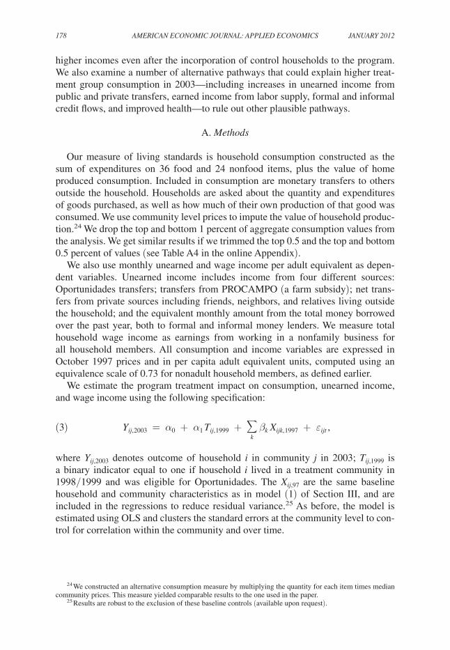
We estimate the program treatment impact on consumption, unearned income, and wage income using the following specification:
(3) y ij, 2003 = α 0 + α 1 t ij, 1999 + ∑ k
β k X ijk, 1997 + ε ijt ,
where yij,2003 denotes outcome of household i in community j in 2003; tij,1999 is a binary indicator equal to one if household i lived in a treatment community in 1998/1999 and was eligible for Oportunidades. The Xij,97 are the same baseline household and community characteristics as in model (1) of Section III, and are included in the regressions to reduce residual variance.25 As before, the model is estimated using OLS and clusters the standard errors at the community level to con-trol for correlation within the community and over time.
24 We constructed an alternative consumption measure by multiplying the quantity for each item times median community prices. This measure yielded comparable results to the one used in the paper.
25 Results are robust to the exclusion of these baseline controls (available upon request).
VOL. 4 NO. 1 179GERtLER Et AL.: INVEStING CASh tRANSFERS
B. Consumption Results
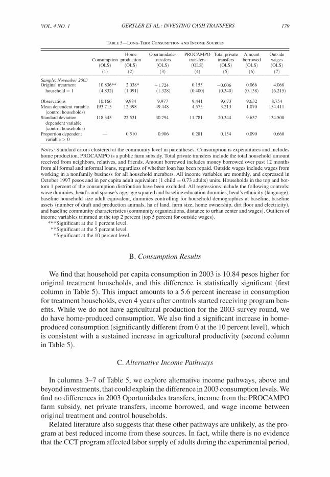
We find that household per capita consumption in 2003 is 10.84 pesos higher for original treatment households, and this difference is statistically significant (first column in Table 5). This impact amounts to a 5.6 percent increase in consumption for treatment households, even 4 years after controls started receiving program ben-efits. While we do not have agricultural production for the 2003 survey round, we do have home-produced consumption. We also find a significant increase in home-produced consumption (significantly different from 0 at the 10 percent level), which is consistent with a sustained increase in agricultural productivity (second column in Table 5).
C. Alternative Income Pathways
In columns 3–7 of Table 5, we explore alternative income pathways, above and beyond investments, that could explain the difference in 2003 consumption levels. We find no differences in 2003 Oportunidades transfers, income from the PROCAMPO farm subsidy, net private transfers, income borrowed, and wage income between original treatment and control households.
Related literature also suggests that these other pathways are unlikely, as the pro-gram at best reduced income from these sources. In fact, while there is no evidence that the CCT program affected labor supply of adults during the experimental period,
Table 5—Long-Term Consumption and Income Sources
Consumption(OLS)
Homeproduction
(OLS)
Oportunidades transfers(OLS)
PROCAMPO transfers(OLS)
Total private transfers(OLS)
Amountborrowed(OLS)
Outside wages(OLS)
(1) (2) (3) (4) (5) (6) (7)
Sample: November 2003Original treatment 10.836** 2.038* −1.724 0.153 −0.006 0.066 4.068 household = 1 (4.832) (1.091) (1.328) (0.400) (0.340) (0.138) (6.215)
Observations 10,166 9,984 9,977 9,441 9,673 9,632 8,754Mean dependent variable (control households)
193.715 12.398 49.448 4.575 3.213 1.070 154.411
Standard deviation dependent variable (control households)
118.345 22.531 30.794 11.781 20.344 9.637 134.508
Proportion dependent variable > 0
— 0.510 0.906 0.281 0.154 0.090 0.660
Notes: Standard errors clustered at the community level in parentheses. Consumption is expenditures and includes home production. PROCAMPO is a public farm subsidy. Total private transfers include the total household amount received from neighbors, relatives, and friends. Amount borrowed includes money borrowed over past 12 months from all formal and informal loans, regardless of whether loan has been repaid. Outside wages include wages from working in a nonfamily business for all household members. All income variables are monthly, and expressed in October 1997 pesos and in per capita adult equivalent (1 child = 0.73 adults) units. Households in the top and bot-tom 1 percent of the consumption distribution have been excluded. All regressions include the following controls: wave dummies, head’s and spouse’s age, age squared and baseline education dummies, head’s ethnicity (language), baseline household size adult equivalent, dummies controlling for household demographics at baseline, baseline assets (number of draft and production animals, ha of land, farm size, home ownership, dirt floor and electricity), and baseline community characteristics (community organizations, distance to urban center and wages). Outliers of income variables trimmed at the top 2 percent (top 5 percent for outside wages).
*** Significant at the 1 percent level. ** Significant at the 5 percent level. * Significant at the 10 percent level.
180 AMERICAN ECONOMIC JOURNAL: APPLIEd ECONOMICS JANUARy 2012
Parker and Skoufias (2000) and Skoufias an Parker (2001) show that it reduced the labor supply of school-age children in salaried and nonsalaried activities, so that they could attend school. Moreover, there is evidence that Oportunidades transfers crowded out some private transfers from relatives and friends during the first year of program exposure (Albarran and Attanasio 2005).
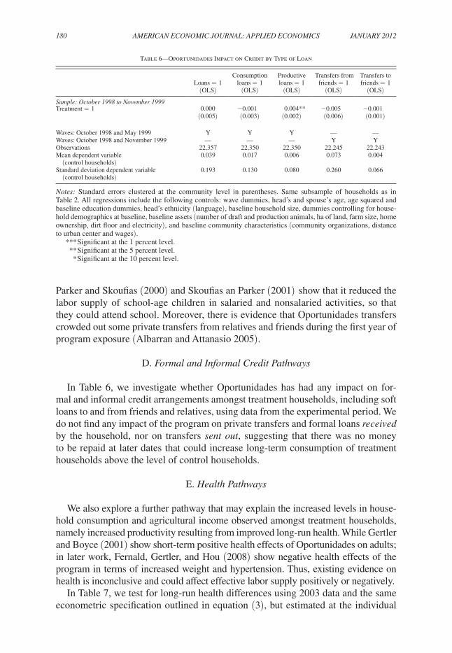
D. Formal and Informal Credit Pathways
In Table 6, we investigate whether Oportunidades has had any impact on for-mal and informal credit arrangements amongst treatment households, including soft loans to and from friends and relatives, using data from the experimental period. We do not find any impact of the program on private transfers and formal loans received by the household, nor on transfers sent out, suggesting that there was no money to be repaid at later dates that could increase long-term consumption of treatment households above the level of control households.
E. health Pathways
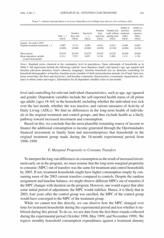
We also explore a further pathway that may explain the increased levels in house-hold consumption and agricultural income observed amongst treatment households, namely increased productivity resulting from improved long-run health. While Gertler and Boyce (2001) show short-term positive health effects of Oportunidades on adults; in later work, Fernald, Gertler, and Hou (2008) show negative health effects of the program in terms of increased weight and hypertension. Thus, existing evidence on health is inconclusive and could affect effective labor supply positively or negatively.
In Table 7, we test for long-run health differences using 2003 data and the same econometric specification outlined in equation (3), but estimated at the individual
Table 6—Oportunidades Impact on Credit by Type of Loan
Loans = 1(OLS)
Consumption loans = 1
(OLS)
Productive loans = 1
(OLS)
Transfers fromfriends = 1
(OLS)
Transfers to friends = 1
(OLS)
Sample: October 1998 to November 1999Treatment = 1 0.000 −0.001 0.004** −0.005 −0.001
(0.005) (0.003) (0.002) (0.006) (0.001)
Waves: October 1998 and May 1999 Y Y Y — —Waves: October 1998 and November 1999 — — — Y YObservations 22,357 22,350 22,350 22,245 22,243Mean dependent variable (control households)
0.039 0.017 0.006 0.073 0.004
Standard deviation dependent variable (control households)
0.193 0.130 0.080 0.260 0.066
Notes: Standard errors clustered at the community level in parentheses. Same subsample of households as in Table 2. All regressions include the following controls: wave dummies, head’s and spouse’s age, age squared and baseline education dummies, head’s ethnicity (language), baseline household size, dummies controlling for house-hold demographics at baseline, baseline assets (number of draft and production animals, ha of land, farm size, home ownership, dirt floor and electricity), and baseline community characteristics (community organizations, distance to urban center and wages).
*** Significant at the 1 percent level. ** Significant at the 5 percent level. * Significant at the 10 percent level.
VOL. 4 NO. 1 181GERtLER Et AL.: INVEStING CASh tRANSFERS
level and controlling for relevant individual characteristics, such as age, age squared and gender. Dependent variables include the self-reported health status of all prime age adults (ages 18–64) in the household, including whether the individual was sick over the last month, whether she was inactive, and various measures of Activity of Daily Living (ADLs). We find no differences in the long-term health of individu-als in the original treatment and control groups, and thus exclude health as a likely pathway toward increased investment and consumption.
Based on this, we conclude that the most plausible remaining source of income to finance the additional consumption is income generated through the Oportunidades financed investment in family farm and microenterprises that households in the original treatment group made during the 18-month experimental period from 1998–1999.
F. Marginal Propensity to Consume transfers
To interpret the long-run differences in consumption as the result of increased invest-ment early on in the program, we must assume that the long-term marginal propensity to consume (MPC) out of transfers was the same for treatment and control households by 2003. If not, treatment households might have higher consumption simply by con-suming more of the 2003 current transfers compared to controls. Despite the random assignment and baseline balance, we might observe different MPCs out of transfers if the MPC changes with duration on the program. However, one would expect that after some initial period of adjustment, the MPC would stabilize. Hence, it is likely that in 2003, four years after the control group was enrolled, the MPC of the control group would have converged to the MPC of the treatment group.
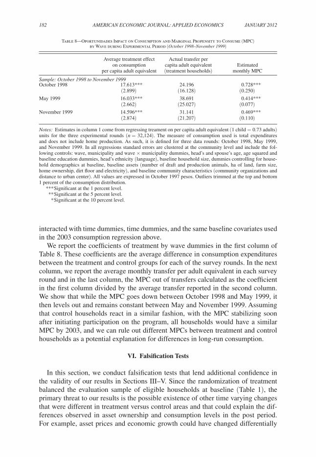
While we cannot test this directly, we can observe how the MPC changed over time for treatment households during the experimental period and test whether it sta-bilized during this period. To do so, we use data from the first three rounds collected during the experimental period (October 1998, May 1999, and November 1999). We regress monthly household consumption expenditures against a treatment dummy
Table 7—Oportunidades Impact on Long-Term Health of Prime Age Adults (18 to 64 years Old)
Sick = 1(OLS)
Numberdays sick(OLS)
Inactivity= 1
(OLS)
Number days
inactivity(OLS)
Number km walk without getting tired
(OLS)
Ability to perform moderate
ADLs(OLS)
Ability to perform vigorous
ADLs(OLS)
Sample: November 2003Original treatment household = 1 0.007 0.113 0.001 −0.074 −0.013 −0.005 −0.007
(0.009) (0.080) (0.005) (0.050) (0.150) (0.008) (0.010)
Observations 24,679 24,679 24,679 24,679 24,253 24,689 24,685Mean dependent variable (control households)
0.131 7.227 0.057 8.138 5.408 1.131 1.194
Notes: Standard errors clustered at the community level in parentheses. Same subsample of households as in Table 5. All regressions include the following controls: wave dummies, head’s and spouse’s age, age squared and baseline education dummies, head’s ethnicity (language), baseline household size ae, dummies controlling for household demographics at baseline, baseline assets (number of draft and production animals, ha of land, farm size, home ownership, dirt floor and electricity), and baseline community characteristics (community organizations, dis-tance to urban center and wages). Information for all dependent variables refers to last month.
182 AMERICAN ECONOMIC JOURNAL: APPLIEd ECONOMICS JANUARy 2012
interacted with time dummies, time dummies, and the same baseline covariates used in the 2003 consumption regression above.
We report the coefficients of treatment by wave dummies in the first column of Table 8. These coefficients are the average difference in consumption expenditures between the treatment and control groups for each of the survey rounds. In the next column, we report the average monthly transfer per adult equivalent in each survey round and in the last column, the MPC out of transfers calculated as the coefficient in the first column divided by the average transfer reported in the second column. We show that while the MPC goes down between October 1998 and May 1999, it then levels out and remains constant between May and November 1999. Assuming that control households react in a similar fashion, with the MPC stabilizing soon after initiating participation on the program, all households would have a similar MPC by 2003, and we can rule out different MPCs between treatment and control households as a potential explanation for differences in long-run consumption.
VI. Falsification Tests
In this section, we conduct falsification tests that lend additional confidence in the validity of our results in Sections III–V. Since the randomization of treatment balanced the evaluation sample of eligible households at baseline (Table 1), the primary threat to our results is the possible existence of other time varying changes that were different in treatment versus control areas and that could explain the dif-ferences observed in asset ownership and consumption levels in the post period. For example, asset prices and economic growth could have changed differentially
Table 8—Oportunidades Impact on Consumption and Marginal Propensity to Consume (MPC) by Wave during Experimental Period (October 1998–November 1999)
Average treatment effecton consumption
per capita adult equivalent
Actual transfer percapita adult equivalent(treatment households)
Estimatedmonthly MPC
Sample: October 1998 to November 1999October 1998 17.613*** 24.196 0.728***
(2.899) (16.128) (0.250)May 1999 16.033*** 38.691 0.414***
(2.662) (25.027) (0.077)November 1999 14.596*** 31.141 0.469***
(2.874) (21.207) (0.110)
Notes: Estimates in column 1 come from regressing treament on per capita adult equivalent (1 child = 0.73 adults) units for the three experimental rounds (n = 32,124). The measure of consumption used is total expenditures and does not include home production. As such, it is defined for three data rounds: October 1998, May 1999, and November 1999. In all regressions standard errors are clustered at the community level and include the fol-lowing controls: wave, municipality and wave × municipality dummies, head’s and spouse’s age, age squared and baseline education dummies, head’s ethnicity (language), baseline household size, dummies controlling for house-hold demographics at baseline, baseline assets (number of draft and production animals, ha of land, farm size, home ownership, dirt floor and electricity), and baseline community characteristics (community organizations and distance to urban center). All values are expressed in October 1997 pesos. Outliers trimmed at the top and bottom 1 percent of the consumption distribution.
*** Significant at the 1 percent level. ** Significant at the 5 percent level. * Significant at the 10 percent level.
VOL. 4 NO. 1 183GERtLER Et AL.: INVEStING CASh tRANSFERS
in treatment and control communities, or other public programs could have been introduced in the treatment areas and not in the control areas.
A specific concern is that the program generated general equilibrium effects that drive changes in investment behavior. Oportunidades infused small rural communi-ties with large amounts of transfers to over half their residents, potentially increas-ing prices in treatment communities. In this scenario, the effects of transfers on increased microenterprise and farm activities shown could simply reflect increases in local prices. However, there is no evidence that differential prices are driving our results. Hoddinot and Skoufias (2004) and Angelucci and De Giorgi (2009) find no differences in food prices in treatment and control communities. In addition, we find no differences in community-level wage rates or animal prices during the experi-mental period (Table A2 in the online Appendix).
We also test for the possibility of differential unobserved time varying factors using the sample of households that were ineligible to participate in Oportunidades based on wealth. If differential time varying changes in unobservable community characteristics explain the differential level of assets and consumption observed in the post-intervention period, then we would also expect to see that ineligible house-holds living in treatment communities have higher asset and consumption levels than ineligible households living in control communities. Hence, we replicate the main analysis in the paper, so far using the sample of ineligibles to help rule out gen-eral equilibrium effects.26 Results reported in the online Appendix, show no effect on agricultural assets and microenterprises (Table A6), no effect on agricultural pro-duction or income (Table A7), and no effect on consumption in 2003 (Table A8). However, we do find an effect on productive loans (sixth column in Table A7), which is consistent with results reported in Angelucci and De Giorgi (2009).
VII. Marginal Propensity to Invest and Long-Run Effects
In this section, we estimate how much of the transfer is consumed versus invested—i.e., the marginal propensity to consume (MPC), and the return on trans-fers in terms of long-term consumption via the investment pathway, which we call the marginal investment effect (MIE). The MPC and the MIE characterize two prin-cipal pathways through which transfers affect living standards. First, households can increase living standards in the short run by spending part of the current cash trans-fer. This amount is just the marginal propensity to consume transfers. Transfers not consumed are saved or invested, so that the marginal propensity to invest transfers is equivalent to (1–MPC). Second, if households indeed invest part of the transfer in productive activities as shown in the previous sections, the return on that invest-ment should yield higher income and consequently increase consumption in future periods. The first pathway represents a temporary increase in living standards that disappears when transfers stop, while the second pathway represents a long-term
26 The subsample of ineligible households includes 3,212 households in treatment communities, and 2,038 households in control communities. To verify that ineligible households were also balanced at baseline, we compare their baseline characteristics, and find no statistical differences in 32 of the 35 key dependent and indepen-dent variables considered (see Table A5 in the online Appendix).
184 AMERICAN ECONOMIC JOURNAL: APPLIEd ECONOMICS JANUARy 2012
improvement in living standards that may be maintained even after the transfers come to an end.
A. Empirical Specification
The basic insight that we use to obtain an empirical specification is that we should be able to extract the MPC and MIE from a model that relates current consumption as a function of current and lagged transfers. We argue that contemporaneous trans-fers affect current consumption if they are used to purchase goods and services, whereas current transfers not used to purchase goods or services in the present are invested, and any increase in income from this investment is realized at a later point in time. In this setting, lagged or past transfers can only affect current consumption if they were invested in productive activities that generate income today.
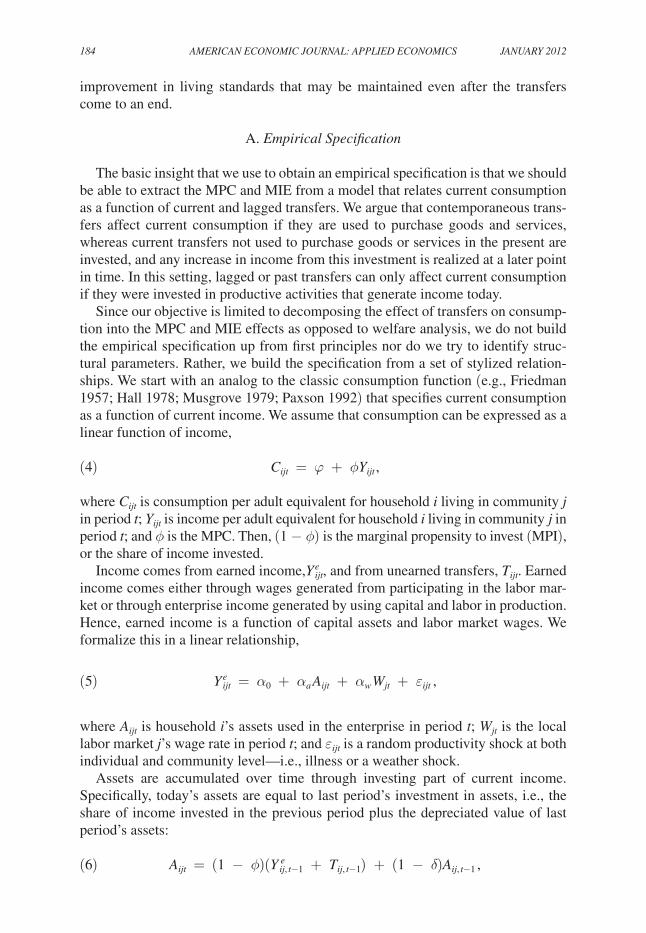
Since our objective is limited to decomposing the effect of transfers on consump-tion into the MPC and MIE effects as opposed to welfare analysis, we do not build the empirical specification up from first principles nor do we try to identify struc-tural parameters. Rather, we build the specification from a set of stylized relation-ships. We start with an analog to the classic consumption function (e.g., Friedman 1957; Hall 1978; Musgrove 1979; Paxson 1992) that specifies current consumption as a function of current income. We assume that consumption can be expressed as a linear function of income,
(4) Cijt = φ + ϕyijt ,
where Cijt is consumption per adult equivalent for household i living in community j in period t; yijt is income per adult equivalent for household i living in community j in period t; and ϕ is the MPC. Then, (1 − ϕ) is the marginal propensity to invest (MPI), or the share of income invested.
Income comes from earned income, y ijt e , and from unearned transfers, tijt. Earned
income comes either through wages generated from participating in the labor mar-ket or through enterprise income generated by using capital and labor in production. Hence, earned income is a function of capital assets and labor market wages. We formalize this in a linear relationship,
(5) y ijt e = α 0 + α a A ijt + α w W jt + ε ijt ,
where Aijt is household i’s assets used in the enterprise in period t; Wjt is the local labor market j’s wage rate in period t; and εijt is a random productivity shock at both individual and community level—i.e., illness or a weather shock.
Assets are accumulated over time through investing part of current income. Specifically, today’s assets are equal to last period’s investment in assets, i.e., the share of income invested in the previous period plus the depreciated value of last period’s assets:
(6) A ijt = (1 − ϕ)( y ij, t−1 e + t ij, t−1 ) + (1 − δ) A ij, t−1 ,
VOL. 4 NO. 1 185GERtLER Et AL.: INVEStING CASh tRANSFERS
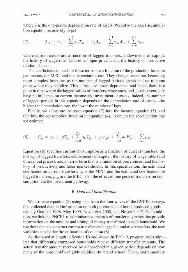
where δ is the one-period depreciation rate of assets. We solve the asset accumula-tion equation recursively to get
(7) A ijt = γ 0 + ∑ s=0
t−1
γ 1s t ijs + γ 2 A ij0 + ∑ s=0
t−1
γ 4s W js + ∑ s=0
t−1
η ijs ,
where current assets are a function of lagged transfers, endowments of capital, the history of wage rates (and other input prices), and the history of productive random shocks.
The coefficients on each of these terms are a function of the production function parameters, the MPC, and the depreciation rate. They change over time, becoming more complex functions as the number of lagged periods grows and up to some point where they stabilize. This is because assets depreciate, and hence there is a point in time where the lagged values of transfers, wage rates, and shocks eventually have no influence on current income and investment or assets. Indeed, the number of lagged periods in this equation depends on the depreciation rate of assets—the higher the depreciation rate, the lower the number of lags.
Finally, we substitute the asset equation (7) into the income equation (5), and that into the consumption function in equation (4), to obtain the specification that we estimate:
(8) C ijt = ρ 0 + ϕ t ijt + ∑ s=0
t−1
ρ 1s t ijs + ρ 2 A ij0 + ∑ s=0
t
ρ 3s W js + ∑ s=0
t
μ ijs .
Equation (8) specifies current consumption as a function of current transfers, the history of lagged transfers, endowments of capital, the history of wage rates (and other input prices), and an error term that is a function of preferences, and the his-tory of productivity and labor market shocks. In this specification, the estimated coefficient on current transfers, ϕ , is the MPC; and the estimated coefficients on lagged transfers, ρ 1s , are the MIE—i.e., the effect of one peso of transfers on con-sumption via the investment pathway.
B. data and Identification
We estimate equation (8) using data from the four waves of the ENCEL surveys that collected detailed information on both purchased and home produced goods—namely October 1998, May 1999, November 2000, and November 2003. In addi-tion, we link the ENCEL to administrative records of transfer payments that provide information on the amount and timing of money transferred to each household. We use these data to construct current transfers and lagged cumulative transfers, the new variables needed for the estimation of equation (8).
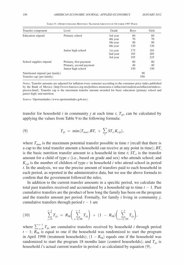
As discussed at length in Section IB and shown in Table 9, program rules stipu-late that differently composed households receive different transfer amounts. The actual transfer amount received by a household in a given period depends on how many of the household’s eligible children do attend school. The actual bimonthly
186 AMERICAN ECONOMIC JOURNAL: APPLIEd ECONOMICS JANUARy 2012
transfer for household i in community j at each time t, tijt, can be calculated by applying the values from Table 9 to the following formula:
(9) t ijt = min ( t max , B t t + ∑ c
S t ct K cijt ),
where tmax is the maximum potential transfer possible in time t (recall that there is a cap to the total transfer amount a household can receive at any point in time); Btt is the basic nutrition transfer amount to a household in time t; Stct is the transfer amount for a child of type c (i.e., based on grade and sex) who attends school; and K cijt is the number of children of type c in household i who attend school in period t. In the analysis, we use the precise amount of transfers paid to each household in each period, as reported in the administrative data, but we use the above formula to confirm that the government followed the rules.
In addition to the current transfer amounts in a specific period, we calculate the total past transfers received and accumulated by a household up to time t − 1. Past cumulative transfers are the product of how long the family has been on the program and the transfer amount per period. Formally, for family i living in community j, cumulative transfers through period t − 1 are
(10) ∑ s=0
t−1
t ijs = R 98 ( ∑ s=4/98
t−1
t ijs ) + (1 − R 98 )( ∑ s=11/99
t−1
t ijs ),
where ∑ s=0 t−1
t ijs are cumulative transfers received by household i through period t − 1; R98 is equal to one if the household was randomized to start the program in April 1998 (treatment households); (1 − R98) equals one if the household was randomized to start the program 18 months later (control households); and tijs is household i’s actual current transfer in period s as calculated by equation (9).
Table 9—Oportunidades Monthly Transfer Amounts in October 1997 Pesos
Transfer component Level Grade Boys Girls
Education stipend Primary school 3rd year 60 604th year 70 705th year 90 906th year 120 120
Junior high school 1st year 175 1852nd year 185 2053rd year 195 225
School supplies stipend Primary, first payment 80 80Primary, second payment 40 40Junior high school 150 150
Nutritional stipend (per family) 90Transfer cap (per family) 550
Notes: Transfer amounts are adjusted for inflation every semester according to the consumer price index published by the Bank of Mexico (http://www.banxico.org.mx/politica-monetaria-e-inflacion/estadisticas/inflacion/indices-precios.html). Transfer cap is the maximum transfer amount awarded for basic education (primary school and junior high) and nutrition.
Source: Oportunidades (www.oportunidades.gob.mx).
VOL. 4 NO. 1 187GERtLER Et AL.: INVEStING CASh tRANSFERS
In equation (8), the coefficient on past cumulative transfers changes the longer in the past the transfer was made. Hence, we do not enter total cumulative past transfers as a single variable. Rather, we enter past transfers, ∑ s=0
t−1 t ijs , in three lagged variables
(s = 1, 2, 3): the amount of transfers the household received in the 12 months prior to the current transfers (s = 1), the amount of transfers the household received from the thirteenth through the twenty-fourth month prior to the current transfers (s = 2), and the amount of transfers the household received more than 24 months prior to the current transfer (s = 3).
One potential concern with this specification is that the current and cumulative transfer amounts that the household actually receives are determined in part by whether children attend school. If a household sends their children to work instead of going to school, then the family would have lower transfers but higher income from the child’s work. This would imply a downward biased estimate of the MPC and an upward biased estimate of the MPI. In reality, this is a concern for our esti-mates given that Parker and Skoufias (2000) and Skoufias and Parker (2001) find that the program reduces child labor and increases enrollment in junior high (sec-ondary) schools as the opportunity cost of these children being in the labor force is now higher. Schultz (2004) also finds positive effects for primary school and, more notably, junior high school enrollment for boys and girls.
We solve this problem by instrumenting current transfers and past cumulative transfers with the maximum potential current and maximum potential past cumula-tive transfers, respectively, that a family could achieve if the maximum number of eli-gible children in the household were enrolled in school.27 At each time t, we compute a family’s maximum potential transfer using a modified version of the formula in (9) and assuming that all eligible children that were enrolled at baseline have advanced a grade per year. Because of the cap on total benefits and because the transfers are zero for the first three years of school, potential transfers are a nonlinear function of the number of children at baseline who could be enrolled in school in period t.
Maximum potential transfers and the three lagged maximum potential cumula-tive transfers are likely to be valid instruments for three reasons. First, they are strong predictors of the actual transfers and the three actual cumulative lagged transfer variables. Indeed, and as expected, the distribution of potential transfers follows that of the actual transfers very closely, albeit potential transfers are an overestimate of the actual transfers (given noncompliance, administrative delays in payments, etc.). The simple correlation amongst both variables is 0.89. After controlling for time effects and baseline covariates, 55.7 and 65.9 percent of the variation in current and cumulative lagged transfers are explained by their poten-tial counterparts.
Second, they are unlikely to be correlated with consumption via other pathways, such as other income sources. Indeed, they are uncorrelated with changes in chil-dren’s labor supply due to the program as they are computed assuming that all eli-gible children enrolled at baseline are still in school and have advanced one school
27 Note that separate identification of current transfers and the three lagged cumulative transfers is possible because cumulative transfers are the product of a randomized variable and a nonlinear function of the number of eligible children attending school, whereas the current transfer only depends on the latter.
188 AMERICAN ECONOMIC JOURNAL: APPLIEd ECONOMICS JANUARy 2012
grade per school year. Nonetheless, the transfers could also be taken in leisure by reducing adult labor supply, which would reduce household income and therefore household consumption. Everything else held constant, this would imply a down-ward biased estimate of the MPC. Parker and Skoufias (2000) show that there is no effect of the program on adult labor supply, and we can thus safely assume that the transfer variables are not correlated with other earned sources of income.
Regarding program impacts on unearned income, the crowding out effect of pri-vate transfers found in Albarran and Attanasio (2005) and discussed earlier, would suggest that our estimated MPC is underestimated. However, private transfers are unlikely to explain our results as the crowding out effects are small in size and, on average, approximately 7.3 percent of eligible households report receiving private transfers over the experimental period (fourth column in Table 6). This proportion doubles to 15.4 percent in November 2003 (see the fifth column in Table 5) suggest-ing that the crowding effects are not sustained over time.
Finally, there is no bias from omitted family demographic structure as we directly control for family structure in the regression models. In fact, maximum potential transfers are not strongly correlated with the number of children in the household because of the nonlinear allocation rule. Let’s imagine the following extreme situ-ations: a household with three girls in grade 2 of primary school, and a household with three girls in grade 2 of junior high school. Both households have three female children, but while the first household will receive no school transfers, the latter household will receive a large monthly transfer. In addition, families with four or more children in junior high school would receive the same transfer amount as the latter household because the cap on total benefits would be binding. Indeed, the data shows low correlations between transfers and the number of children under 17 (r = 0.14), or with the number of siblings 15–17 years old (r = 0.42), 12–14 years old (r = 0.22), 6–11 years old (r = −0.12), and 0–5 years old (r = −0.10). Thus, we are able to explicitly control for household size and the number of children in the household in the empirical specification, which allows for identification of the potential transfer variable.
We measure human and physical capital endowments at baseline (1997) before treatment households start receiving transfers. Specifically, we control for head’s and spouse’s age, education, and ethnicity, as well as adult equivalent household size and composition. Note that the latter variables also adjust for any economies of scale in consumption. We also control for pre-intervention home ownership, dirt floor, electricity, the number of draft and production animals, and hectares of land in use. Finally, we control for wages and inputs prices using municipality dummies interacted with wave dummies.
C. Results
We estimate equation (8) by two-stage least squares (2SLS) clustering the standard errors at the community level to control for the correlation of shocks within communi-ties over time. The first column of Table 10 presents the 2SLS estimates of the MPC and the MIE. For the sake of comparison, we report OLS estimates in the second col-umn, which, as expected, are substantially lower than their 2SLS counterparts.
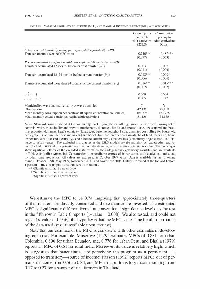
VOL. 4 NO. 1 189GERtLER Et AL.: INVEStING CASh tRANSFERS
We estimate the MPC to be 0.74, implying that approximately three-quarters of the transfers are directly consumed and one-quarter are invested. The estimated MPC is significantly different from 1 at conventional significance levels, as the test in the fifth row in Table 6 reports ( p-value = 0.008). We also tested, and could not reject ( p-value of 0.956), the hypothesis that the MPC is the same for all four rounds of the data used (results available upon request).
Note that our estimate of the MPC is consistent with other estimates in develop-ing countries. For example, Musgrove (1979) estimates MPCs of 0.881 for urban Colombia, 0.896 for urban Ecuador, and, 0.776 for urban Peru; and Bhalla (1979) reports an MPC of 0.61 for rural India. Moreover, its value is relatively high, which is suggestive that beneficiaries are perceiving the program as a permanent—as opposed to transitory—source of income: Paxson (1992) reports MPCs out of per-manent income from 0.56 to 0.84, and MPCs out of transitory income ranging from 0.17 to 0.27 for a sample of rice farmers in Thailand.
Table 10—Marginal Propensity to Consume (MPC) and Marginal Investment Effect (MIE) on Consumption
Consumption per capita
adult equivalent(2SLS)
Consumption per capita
adult equivalent(OLS)
Actual current transfer (monthly per capita adult equivalent)—MPCTransfer amount (average MPC = ϕ ) 0.740*** 0.487***
(0.097) (0.059)Past accumulated transfers (monthly per capita adult equivalent)—MIETransfers accumlated 12 months before current transfer ( ρ 11) 0.003 0.007
(0.011) (0.006)Transfers accumlated 13–24 months before current transfer ( ρ 12) 0.018*** 0.008*
(0.006) (0.004)Transfers accumlated more than 24 months before current transfer ( ρ 13) 0.016*** 0.015***
(0.002) (0.002)
p( ϕ ) = 1 0.008 0.000p( ρ 12 = ρ 13) 0.805 0.147
Municipality, wave and municipality × wave dummies Y YObservations 42,139 42,139Mean monthly consumption per capita adult equivalent (control households) 164.778 164.778Mean monthly actual transfer per capita adult equivalent 31.136 31.136
Notes: Standard errors clustered at the community level in parentheses. All regressions include the following set of controls: wave, municipality and wave × municipality dummies, head’s and spouse’s age, age squared and base-line education dummies, head’s ethnicity (language), baseline household size, dummies controlling for household demographics at baseline, baseline assets (number of draft and production animals, ha of land, farm size, home ownership, dirt floor and electricity), and baseline community characteristics (community organizations and dis-tance to urban center). The excluded instruments in the 2SLS models are the monthly per capita adult equiva-lent (1 child = 0.73 adults) potential transfers and the three lagged cumulative potential transfers. The first stages show significant effects of the excluded instruments on the endogeneous explanatory variables and are available in Table A10 (online Appendix). Consumption is expenditures expressed in per capita adult equivalent units, and includes home production. All values are expressed in October 1997 pesos. Data is available for the following rounds: October 1998, May 1999, November 2000, and November 2003. Outliers trimmed at the top and bottom 1 percent of the consumption and transfers distributions.
*** Significant at the 1 percent level. ** Significant at the 5 percent level. * Significant at the 10 percent level.
190 AMERICAN ECONOMIC JOURNAL: APPLIEd ECONOMICS JANUARy 2012
The next three rows in Table 10 report the estimated coefficients on the three lagged cumulative transfer variables and are the estimates of the MIE. The first coefficient, ρ 11 , represents the effect on consumption from transfers made in the 12 months prior to the current transfer. This coefficient is small and not significantly different from zero. This is consistent with the notion that investments take time before they become productive. Indeed, investments made within the last 12 months do not seem to generate enough income to affect consumption. The second coef-ficient, ρ 12 , represents the effect on consumption of transfers made in the second 12-month period prior to the current transfers. This coefficient is positive and sig-nificantly different from zero. We estimate that for every peso transferred during this period, current consumption increased by 1.8 cents. The third coefficient represents the effect on consumption of transfers made in the period prior to 24 months before the current transfer period. This coefficient is positive and significantly different from zero, and implies that for every peso transferred during this period, current consumption increased by 1.6 cents. While this coefficient is slightly lower than the second lag, the two are not significantly different from one another, as reported in the sixth row of Table 10 ( p-value = 0.805). This suggests at best a slight drop off in the MIE due to depreciation.
Using these estimates of MPC and MIE, we run a back-of-the-envelope calcula-tion to predict the long-term effects of the cash transfers on living standards, sim-ply multiplying the MIE by total cumulative transfers. By November 2003, after 51/2 years on the program, households in the treatment group had received a total of 2,624 pesos per capita, on average.28 Using our more conservative estimate of the MIE of 0.016, this implies an increase in consumption of 41.9 pesos per capita per month through the investment pathway. This amounts to an approximately 21.8 per-cent increase in consumption. If these increases in consumption are, as argued here, derived from productive investments made by beneficiary households thanks to the cash transfers, then to the extent that the investments are long term, these increases in living standards are expected to be sustained over time even after the household is no longer receiving cash transfers from Oportunidades.
VIII. Conclusions
Conditional cash transfer programs such as Mexico’s Oportunidades are designed to alleviate short-term poverty through cash while incentivizing families to invest in the human capital of the next generation. The positive benefits of this type of pro-gram are well established—including increased caloric intake, better health and nutri-tion, and higher school enrollment for children (see Fiszbein and Schady 2009 for a review). This increased human capital is expected to play an important role in break-ing the cycle of poverty for younger generations. This paper shows that there are also more immediate implications of cash transfers for alleviating long-term poverty for the current generation of beneficiary households. Cash transfers appear to increase living standards permanently by facilitating investments in productive activities.
28 Author’s calculations using transfer payments records.
VOL. 4 NO. 1 191GERtLER Et AL.: INVEStING CASh tRANSFERS
Using data from a controlled randomized experiment, we provide evidence that beneficiaries invested part of their payments in productive activities and that these investments increased income streams. We also find that the stream of income generated from these investments is sustained over time, thereby raising long-term living standards as measured by consumption. Specifically, we find that four years after the control groups were incorporated into the program, consumption levels for the original treatment households were 5.6 percent higher than for the original control households. This result suggests that returns on investments made by treat-ment households in the initial 18-month experimental period did in fact translate into improvements in long-term living standards. As a result, if removed from the program, beneficiary households would most likely not revert to pre-program pov-erty levels. Given that households are granted a minimum of nine years of program benefits, the investment of Oportunidades cash transfers is likely to have a large and significant effect on raising long-term living standards.
REFERENCES
Aghion, Philippe, and Patrick Bolton. 1997. “A Theory of Trickle-Down Growth and Development.” Review of Economic Studies, 64(2): 151–72.
Albarran, Pedro, and Orazio P. Attanasio. 2005. “Do Public Transfers Crowd out Private Transfers? Evidence from a Randomized Experiment in Mexico.” In Insurance Against Poverty, ed. Stefan Dercon, 281–304. Oxford: Oxford University Press.
Angelucci, Manuela, and Orazio Attanasio. 2009. “Oportunidades: Program Effect on Consumption, Low Participation, and Methodological Issues.” Economic development and Cultural Change, 57(3): 479–506.
Angelucci, Manuela, and Giacomo De Giorgi. 2009. “Indirect Effects of an Aid Program: How Do Cash Transfers Affect Ineligibles’ Consumption?” American Economic Review, 99(1): 486–508.
Attanasio, Orazio, and Alice Mesnard. 2006. “The Impact of a Conditional Cash Transfer Programme on Consumption in Colombia.” Fiscal Studies, 27(4): 421–42.
Attanasio, Orazio, Costas Meghir, and Ana Santiago. Forthcoming. “Education Choices in Mexico: Using a Structural Model and a Randomized Experiment to Evaluate Progresa.” Review of Economic Studies.
Banerjee, Abhijit V. 2004. “Contracting Constraints, Credit Markets, and Economic Development.” In Advances in Economics and Econometrics: theory and Applications, Eighth World Congress, Vol. 3, ed. Mathias Dewatripont, Lars Peter Hansen, and Stephen J. Turnovsky, 1–46. Cambridge, UK: Cambridge University Press.
Banerjee, Abhijit V., and Andrew F. Newman. 1993. “Occupational Choice and the Process of Devel-opment.” Journal of Political Economy, 101(2): 274–98.
Behrman, Jere R., and Petra E. Todd. 1999. “Randomness in the Experimental Samples of PRO-GRESA.” International Food Policy Research Institute (IFPRI) Report. Washington DC, March.
Bhalla, Surjit S. 1979. “Measurement Errors and the Permanent Income Hypothesis: Evidence from Rural India.” American Economic Review, 69(3): 295–307.
Di Maro, Vincenzo. 2004. “Evaluation of the Impact of PROGRESA on Nutrition: Theory, Econo-metric Methods and an Approach to Deriving Individual Welfare Findings from Household Data.” www.vincenzodimaro.it/pdf/progresa_fcons_dimaro.pdf.
Fernald, Lia C. H., Paul J. Gertler, and Xiaohui Hou. 2008. “Cash Component of Conditional Cash Transfer Program Is Associated with Higher Body Mass Index and Blood Pressure in Adults.” Jour-nal of Nutrition, 138(11): 2250–57.
Fiszbein, Ariel, and Norbert Schady. 2009. Conditional Cash transfers: Reducing Present and Future Poverty. Washington DC: The World Bank.
Friedman, Milton. 1957. A theory of the Consumption Function. Princeton: Princeton University Press.
Gertler, Paul J., and Simone Boyce. 2001. “An Experiment in Incentive-Based Welfare: The Impact of PROGRESA on Health in Mexico.” http://faculty.haas.berkeley.edu/gertler/working_papers/PRO-GRESA%204-01.pdf.
192 AMERICAN ECONOMIC JOURNAL: APPLIEd ECONOMICS JANUARy 2012
Gertler, Paul J., Sebastian W. Martinez, and Marta Rubio-Codina. 2012. “Investing Cash Transfers to Raise Long-Term Living Standards: Dataset.” American Economic Journal: Applied Economics. http://dx.doi.org/10.1257/app.4.1.164.
Hall, Robert E. 1978. “Stochastic Implications of the Life Cycle-Permanent Income Hypothesis: The-ory and Evidence.” Journal of Political Economy, 86(6): 971–87.
Hoddinott, John, and Emmanuel Skoufias. 2004. “The Impact of PROGRESA on Food Consumption.” Economic development and Cultural Change, 53(1): 37–61.
Lindh, Thomas, and Henry Ohlsson. 1998. “Self-Employment and Wealth Inequality.” Review of Income and Wealth, 44(1): 25–42.
Lloyd-Ellis, Huw, and Dan Bernhardt. 2000. “Enterprise, Inequality and Economic Development.” Review of Economic Studies, 67(1): 147–68.
McKenzie, David J., and Christopher Woodruff. 2006. “Do Entry Costs Provide an Empirical Basis for Poverty Traps? Evidence from Mexican Microenterprises.” Economic development and Cul-tural Change, 55(1): 3–42.
Musgrove, Philip. 1979. “Permanent Household Income and Consumption in Urban South America.” American Economic Review, 69(3): 355–68.
Oportunidades. 2003. “Reglas de Operación 2003.” http://www.oportunidades.gob.mx/Portal/work/sites/web/resources/ArchivoContent/524/Reglas_operacion_2003.pdf.
Oportunidades. 2011. http://www.oportunidades.gob.mx/Portal/wb/Web/poblacion_objetivo_y_mon-tos_asignados_para_el_ejer.
Parker, Susan W., and Emmanuel Skoufias. 2000. “The Impact of PROGRESA on Work, Leisure, and Time Allocation.” International Food Policy Research Institute (IFPRI) Report. Washington DC, October.
Paxson, Christina H. 1992. “Using Weather Variability to Estimate the Response of Savings to Transi-tory Income in Thailand.” American Economic Review, 82(1): 15–33.
Ravallion, Martin, and Shaohua Chen. 2005. “Hidden Impact? Household Saving in Response to a Poor-Area Development Project.” Journal of Public Economics, 89(11–12): 2183–2204.
Sadoulet, Elisabeth, Alain de Janvry, and Benjamin Davis. 2001. “Cash Transfer Programs with Income Multipliers: PROCAMPO in Mexico.” World development, 29(6): 1043–56.
Schultz, T. Paul. 2004. “School Subsidies for the Poor: Evaluating the Mexican Progresa Poverty Pro-gram.” Journal of development Economics, 74(1): 199–250.
Skoufias, Emmanuel, Benjamin Davis, and Sergio de la Vega. 2001. “Targeting the Poor in Mexico: An Evaluation of the Selection of Households into PROGRESA.” World development, 29(10): 1769–84.
Skoufias, Emmanuel, and Susan W. Parker. 2001. “Conditional Cash Transfers and Their Impact on Child Work and Schooling: Evidence from the PROGRESA Program in Mexico.” Economia, 2(1): 45–86.
Stecklov, Guy, Paul Winters, Jessica Todd, and Ferdinando Regalia. 2007. “Unintended Effects of Poverty Programmes on Childbearing in Less Developed Countries: Experimental Evidence from Latin America.” Population Studies, 61(2): 125–40.
Woodruff, Christopher, and Rene Zenteno. 2007. “Migration Networks and Microenterprises in Mex-ico.” Journal of development Economics, 82(2): 509–28.
Yang, Dean. 2008. “International Migration, Remittances and Household Investment: Evidence from Philippine Migrants’ Exchange Rate Shocks.” Economic Journal, 118(528): 591–630.

This article has been cited by:
1. Gustavo J. Bobonis,, Melissa González-Brenes,, Roberto Castro. 2013. Public Transfers andDomestic Violence: The Roles of Private Information and Spousal Control. American EconomicJournal: Economic Policy 5:1, 179-205. [Abstract] [View PDF article] [PDF with links]