Embed Size (px)
Citation preview
1
Weighted Residual
Methods
2
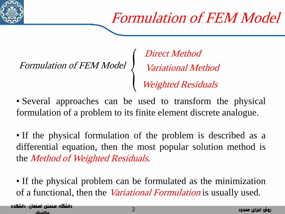
Formulation of FEM Model Direct Method
Variational Method
Weighted Residuals
Formulation of FEM Model
• Several approaches can be used to transform the physical
formulation of a problem to its finite element discrete analogue.
• If the physical formulation of the problem is described as a
differential equation, then the most popular solution method is
the Method of Weighted Residuals.
• If the physical problem can be formulated as the minimization
of a functional, then the Variational Formulation is usually used.
Finite element method is used to solve physical problems
Solid Mechanics
Fluid Mechanics
Heat Transfer
Electrostatics
Electromagnetism
….
Physical problems are governed by differential equations which satisfy
Boundary conditions
Initial conditions
One variable: Ordinary differential equation (ODE)
Multiple independent variables: Partial differential equation (PDE)
3
Formulation of FEM Model
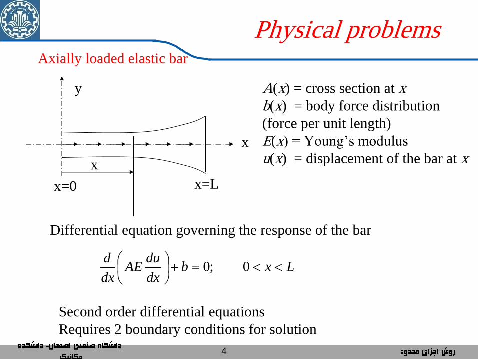
Axially loaded elastic bar
x
y
x=0 x=L
A(x) = cross section at x
b(x) = body force distribution
(force per unit length)
E(x) = Young’s modulus
u(x) = displacement of the bar at x x
Differential equation governing the response of the bar
Lxbdx
duAE
dx
d
0;0
Second order differential equations
Requires 2 boundary conditions for solution
4
Physical problems
5
x
y
x=0 x=L
x
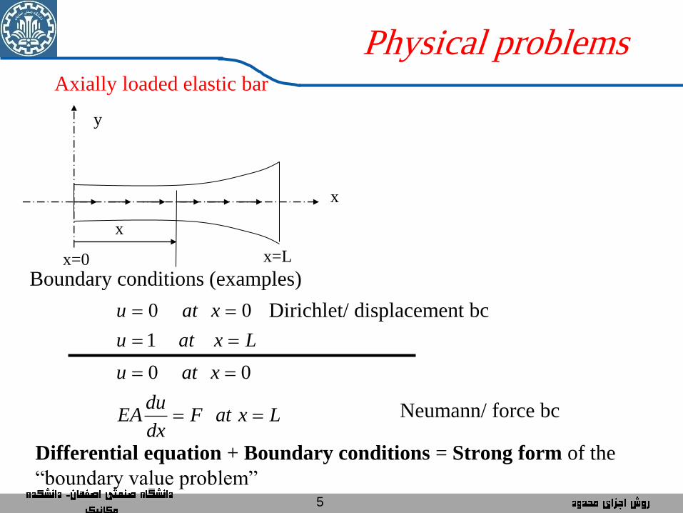
Boundary conditions (examples)
Lxatu
xatu
1
00 Dirichlet/ displacement bc
LxatFdx
duEA
xatu
00
Neumann/ force bc
Differential equation + Boundary conditions = Strong form of the
“boundary value problem”
Physical problems Axially loaded elastic bar
6
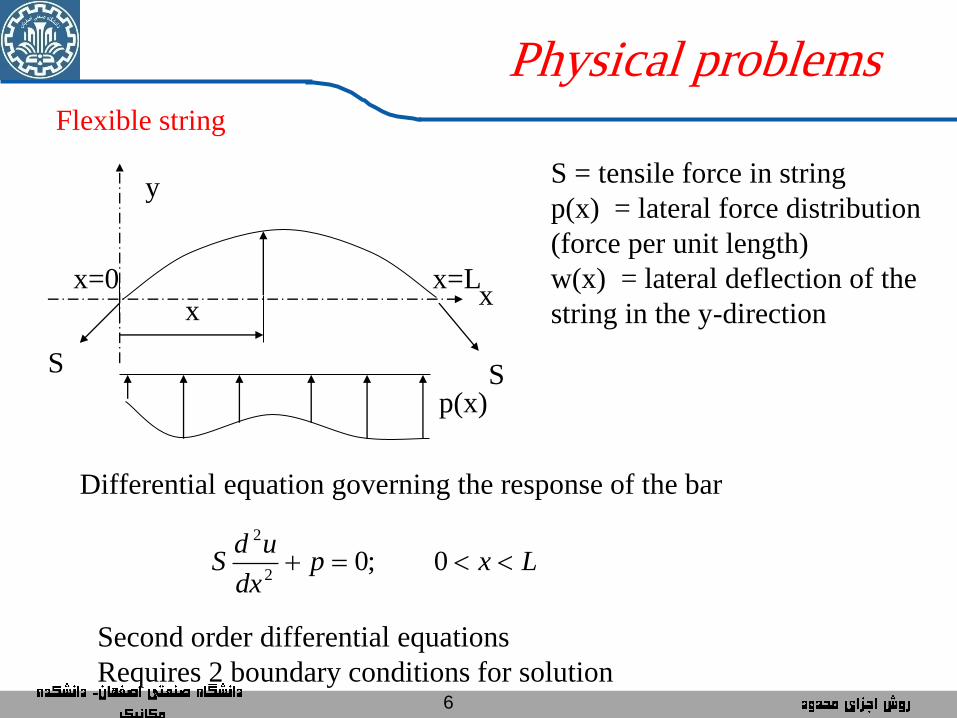
Flexible string
x
y
x=0 x=L x
S S p(x)
S = tensile force in string
p(x) = lateral force distribution
(force per unit length)
w(x) = lateral deflection of the
string in the y-direction
Differential equation governing the response of the bar
Lxpdx
udS 0;0
2
2
Second order differential equations
Requires 2 boundary conditions for solution
Physical problems
7
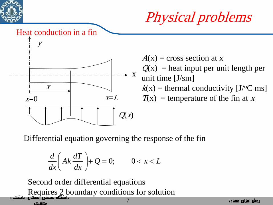
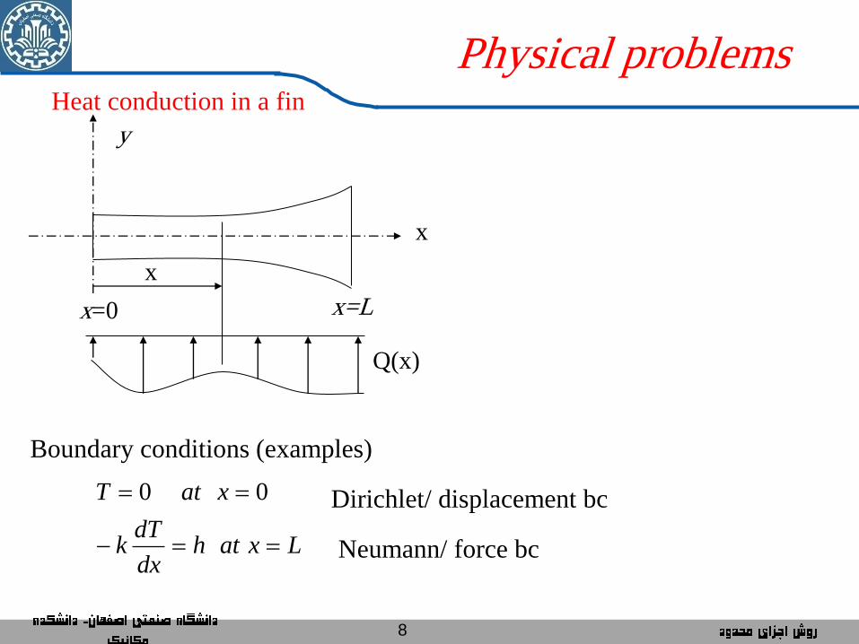
Heat conduction in a fin
Differential equation governing the response of the fin
Second order differential equations
Requires 2 boundary conditions for solution
A(x) = cross section at x
Q(x) = heat input per unit length per
unit time [J/sm]
k(x) = thermal conductivity [J/oC ms]
T(x) = temperature of the fin at x
x
y
x=0 x=L
x
Q(x)
LxQdx
dTAk
dx
d
0;0
Physical problems
8
Boundary conditions (examples)
Dirichlet/ displacement bc
Lxathdx
dTk
xatT
00
Neumann/ force bc
x
y
x=0 x=L
x
Q(x)
Physical problems Heat conduction in a fin
9
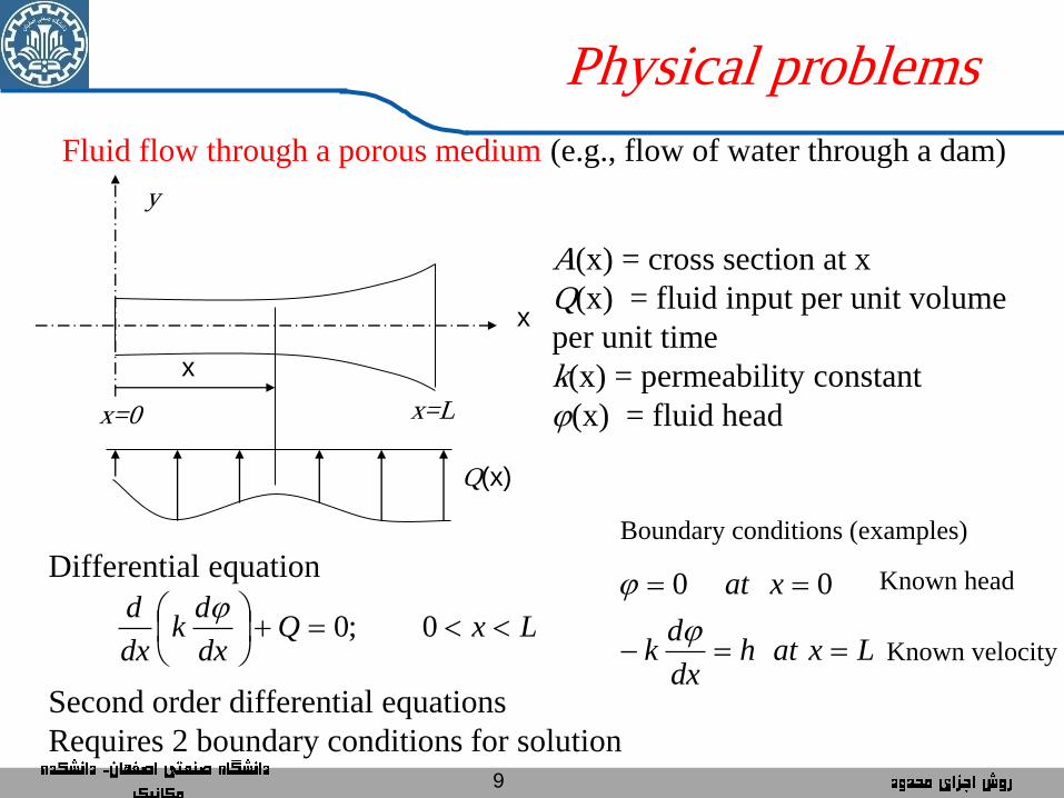
Fluid flow through a porous medium (e.g., flow of water through a dam)
Differential equation
Second order differential equations
Requires 2 boundary conditions for solution
A(x) = cross section at x
Q(x) = fluid input per unit volume
per unit time
k(x) = permeability constant
j(x) = fluid head
x
y
x=0 x=L
x
Q(x)
LxQdx
dk
dx
d
0;0
j
Physical problems
Boundary conditions (examples)
Known head
Lxathdx
dk
xat
j
j 00
Known velocity
10
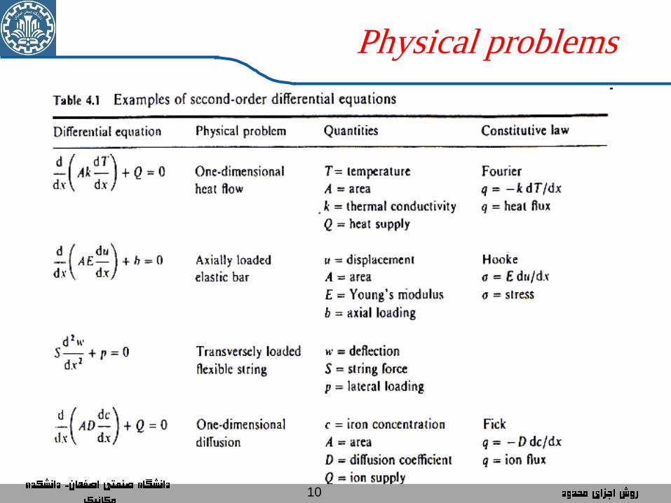
Physical problems
11
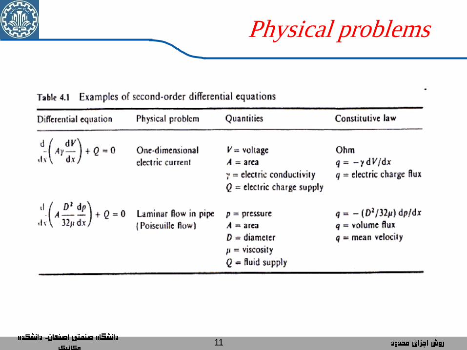
Physical problems
12
Observe:
1. All the cases we considered lead to very similar differential
equations and boundary conditions.
2. In 1D it is easy to analytically solve these equations
3. Not so in 2 and 3D especially when the geometry of the domain is
complex: need to solve approximately
4. We’ll learn how to solve these equations in 1D. The approximation
techniques easily translate to 2 and 3D, no matter how complex the
geometry
Formulation of FEM Model
13
Finite Element Method
Integral Formulation
14
Some Mathematical Concepts
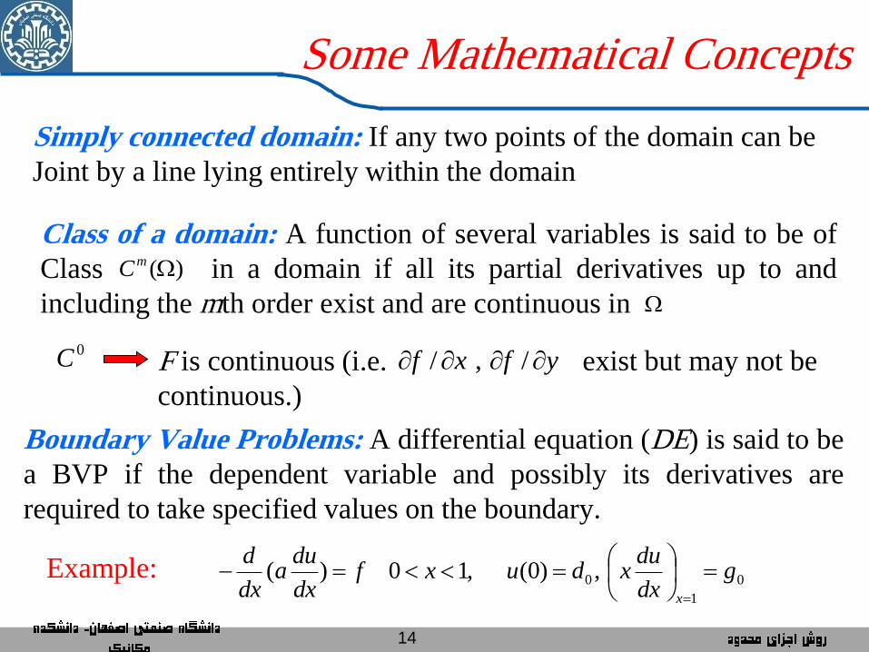
Simply connected domain: If any two points of the domain can be
Joint by a line lying entirely within the domain
Class of a domain: A function of several variables is said to be of
Class in a domain if all its partial derivatives up to and
including the mth order exist and are continuous in
)(mC
0C F is continuous (i.e. exist but may not be
continuous.)
yfxf / , /
Boundary Value Problems: A differential equation (DE) is said to be
a BVP if the dependent variable and possibly its derivatives are
required to take specified values on the boundary.
0
1
0 , )0(,10 )( gdx
duxduxf
dx
dua
dx
d
x
Example:
15
Some Mathematical Concepts
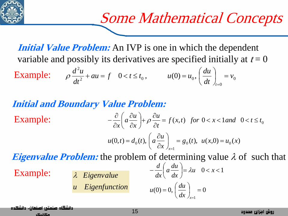
Initial Value Problem: An IVP is one in which the dependent
variable and possibly its derivatives are specified initially at t = 0
0
0
002
2
, )0(,0 vdt
duuuttfau
dt
ud
t
Example:
Initial and Boundary Value Problem:
)()0,(), (), (),0(
0 10 ) ,(
00
1
0
0
xuxutgx
uatdtu
ttandxfortxft
u
x
ua
x
x
Eigenvalue Problem: the problem of determining value l of such that
0, 0)0(
10
1
xdx
duu
xudx
dua
dx
dl
ionEigenfunctu
Eigenvalue
l
Example:
Example:
16
Some Mathematical Concepts
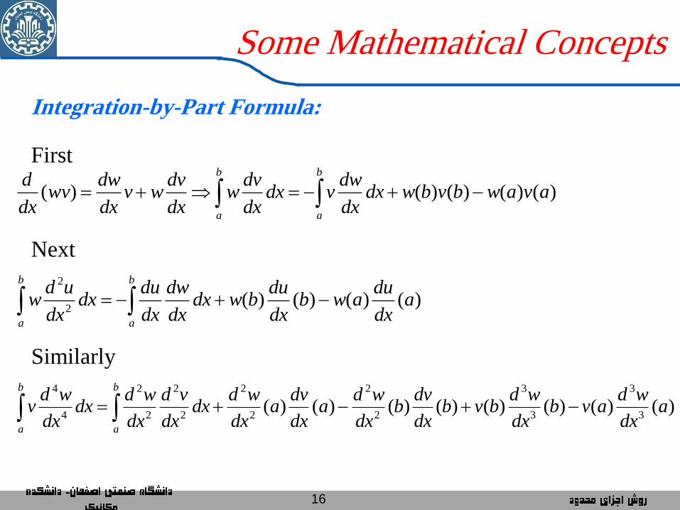
Integration-by-Part Formula:
)()()()()( avawbvbwdxdx
dwvdx
dx
dvw
dx
dvwv
dx
dwwv
dx
db
a
b
a
Next
First
)()()()(2
2
adx
duawb
dx
dubwdx
dx
dw
dx
dudx
dx
udw
b
a
b
a
Similarly
)()()()()()()()(3
3
3
3
2
2
2
2
2
2
2
2
4
4
adx
wdavb
dx
wdbvb
dx
dvb
dx
wda
dx
dva
dx
wddx
dx
vd
dx
wddx
dx
wdv
b
a
b
a
17
Some Mathematical Concepts
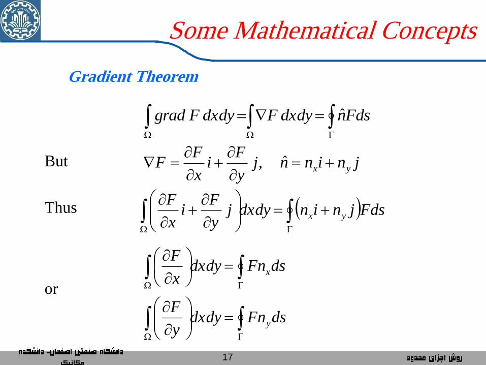
Gradient Theorem
FdsndxdyFdxdyFgrad ˆ
But jninnjy
Fi
x
FF yx
ˆ,
Thus
Fdsjnindxdyj
y
Fi
x
Fyx
or
dsFndxdyy
F
dsFndxdyx
F
y
x
18
Some Mathematical Concepts
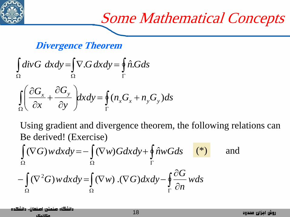
Divergence Theorem
GdsndxdyGdxdydivG .ˆ .
dsGnGndxdy
y
G
x
Gyyxx
yx )(
Using gradient and divergence theorem, the following relations can
Be derived! (Exercise)
wGdsnGdxdywdxdywG ˆ) ( ) ( and
wds
n
GdxdyGwdxdywG )) .(( ) ( 2
(*)
19
Some Mathematical Concepts
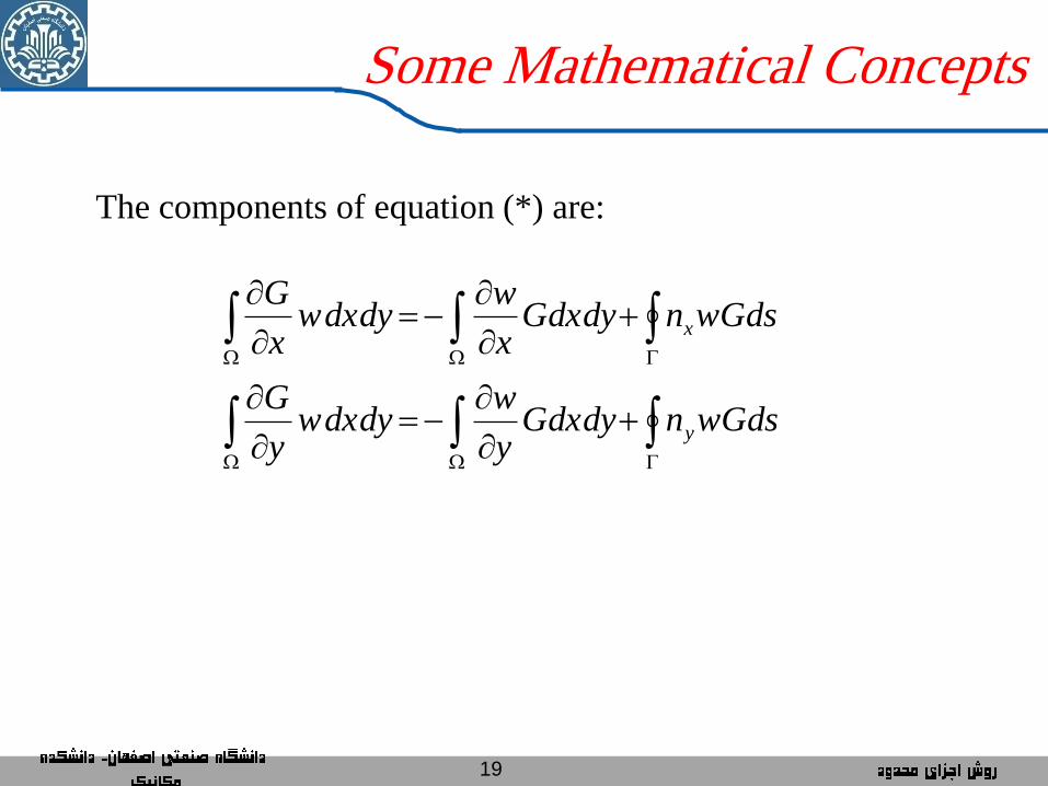
The components of equation (*) are:
wGdsnGdxdyy
wdxdyw
y
G
wGdsnGdxdyx
wdxdyw
x
G
y
x
20
Some Mathematical Concepts
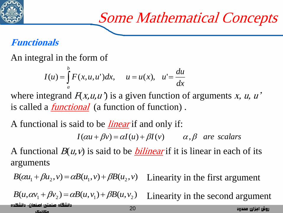
An integral in the form of
b
adx
duuxuudxuuxFuI '), (, )',,()(
where integrand F(x,u,u’) is a given function of arguments x, u, u’
is called a functional (a function of function) .
A functional is said to be linear if and only if:
)()()( vIuIvuI scalarsare ,
A functional B(u,v) is said to be bilinear if it is linear in each of its
arguments
),(),(),( 2121 vuBvuBvuuB Linearity in the first argument
),(),(),( 2121 vuBvuBvvuB Linearity in the second argument
Functionals
21
Some Mathematical Concepts
Functionals
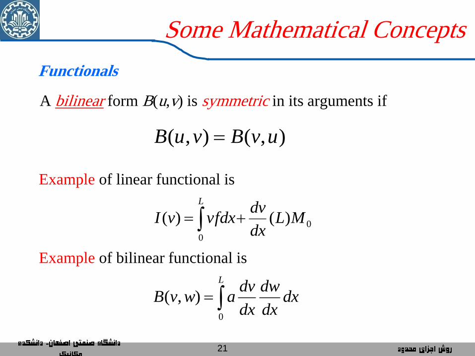
A bilinear form B(u,v) is symmetric in its arguments if
),(),( uvBvuB
Example of linear functional is
L
MLdx
dvvfdxvI
0
0)()(
Example of bilinear functional is
L
dxdx
dw
dx
dvawvB
0
),(
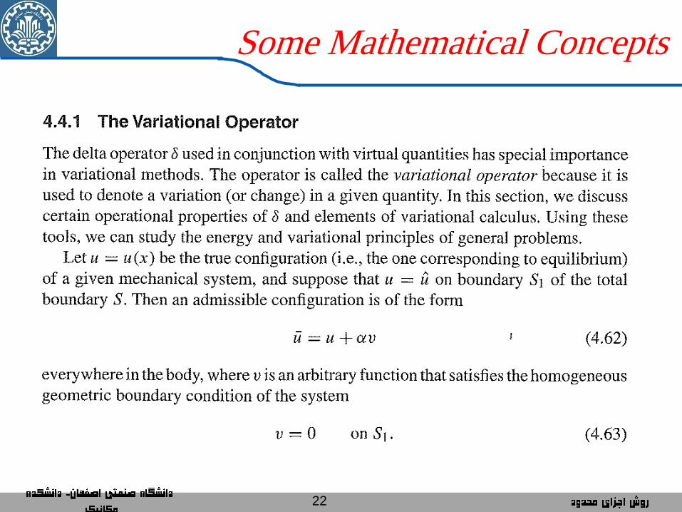
22
Some Mathematical Concepts
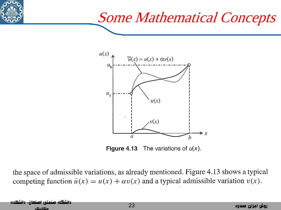
23
Some Mathematical Concepts
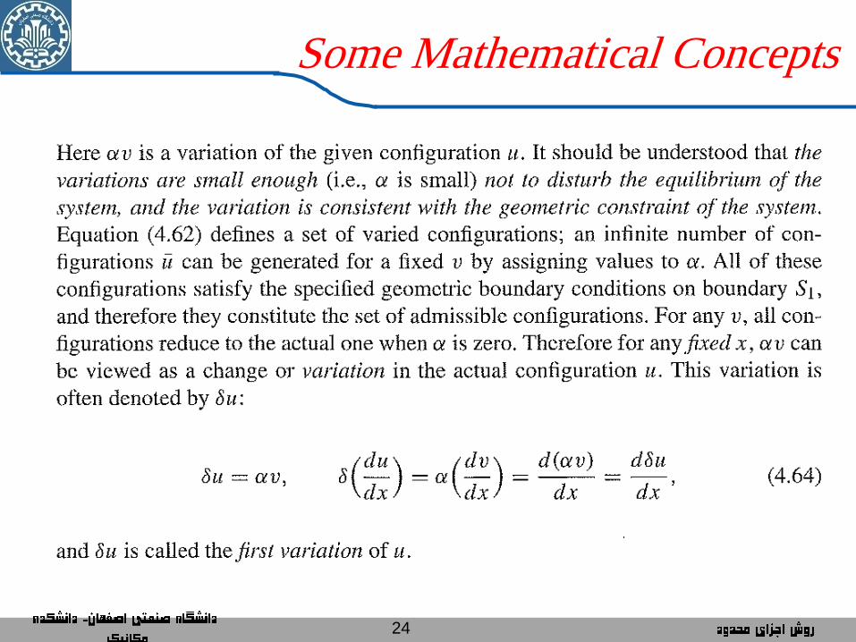
24
Some Mathematical Concepts
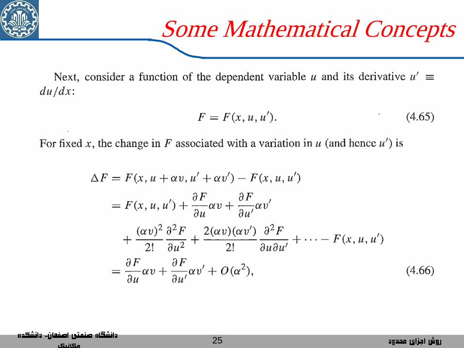
25
Some Mathematical Concepts
26
Some Mathematical Concepts
27
Some Mathematical Concepts
28
Some Mathematical Concepts
29
Some Mathematical Concepts
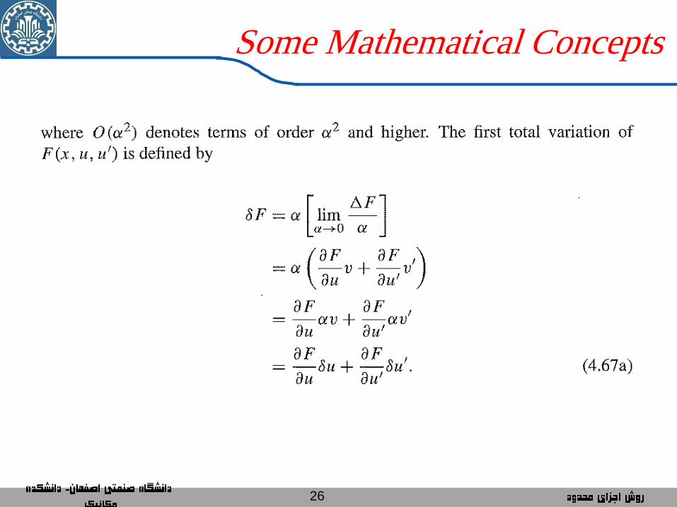
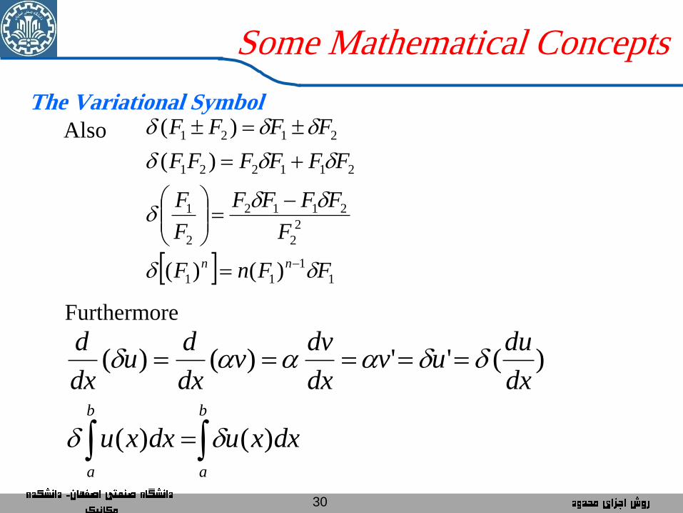
Consider the function )',,( uuxFF for fixed value of x, F only
depends on
The change v in u, where is constant and v is a function, is
called variation of u and denoted by:
vu Variational Symbol
''
uu
Fu
u
FF
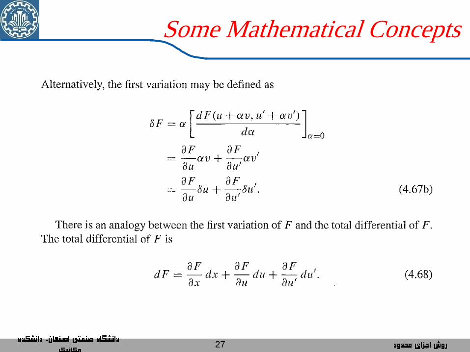
In analogy with the total differential of a function
Note that
''du
u
Fdu
u
Fdx
x
FdF
The Variational Symbol
',uu
30
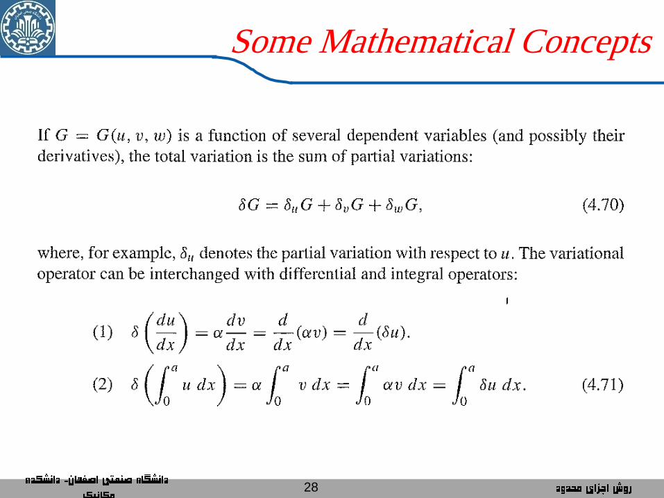
Some Mathematical Concepts
1
1
11
2
2
2112
2
1
211221
2121
)()(
)(
)(
FFnF
F
FFFF
F
F
FFFFFF
FFFF
nn
Also
Furthermore
b
a
b
a
dxxudxxu
dx
duuv
dx
dvv
dx
du
dx
d
)()(
)('')()(
The Variational Symbol
31
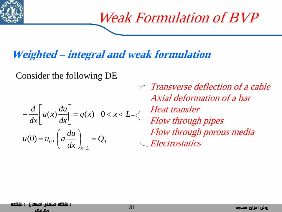
Weak Formulation of BVP
Weighted – integral and weak formulation
00 , )0(
0) ()(
Qdx
duauu
Lxxqdx
duxa
dx
d
Lx
Consider the following DE
Transverse deflection of a cable
Axial deformation of a bar
Heat transfer
Flow through pipes
Flow through porous media
Electrostatics
32
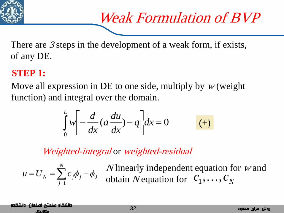
Weak Formulation of BVP
There are 3 steps in the development of a weak form, if exists,
of any DE.
STEP 1:
Move all expression in DE to one side, multiply by w (weight
function) and integral over the domain.
L
dxqdx
dua
dx
dw
0
0)(
Weighted-integral or weighted-residual
N
j
jjN cUu1
0N linearly independent equation for w and
obtain N equation for Ncc ,,1
(+)
33
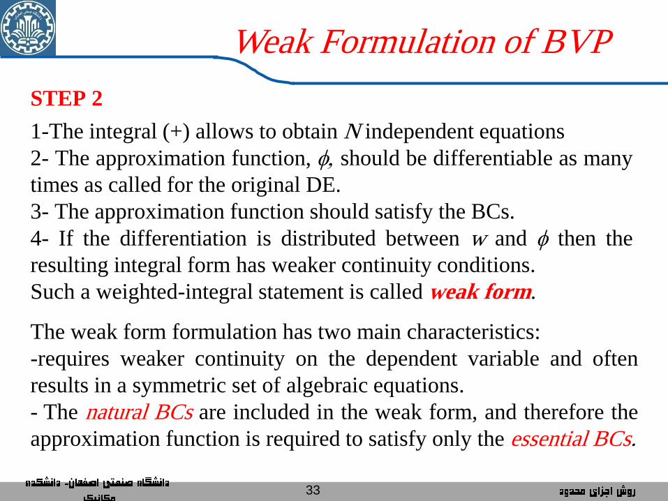
Weak Formulation of BVP
STEP 2
1-The integral (+) allows to obtain N independent equations
2- The approximation function, , should be differentiable as many
times as called for the original DE.
3- The approximation function should satisfy the BCs.
4- If the differentiation is distributed between w and then the
resulting integral form has weaker continuity conditions.
Such a weighted-integral statement is called weak form.
The weak form formulation has two main characteristics:
-requires weaker continuity on the dependent variable and often
results in a symmetric set of algebraic equations.
- The natural BCs are included in the weak form, and therefore the
approximation function is required to satisfy only the essential BCs.
34
Weak Formulation of BVP
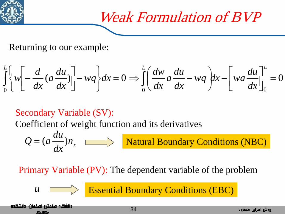
Returning to our example:
0 0)(000
LLL
dx
duwadxwq
dx
dua
dx
dwdxwq
dx
dua
dx
dw
Secondary Variable (SV):
Coefficient of weight function and its derivatives
xndx
duaQ )( Natural Boundary Conditions (NBC)
Primary Variable (PV): The dependent variable of the problem
u Essential Boundary Conditions (EBC)
35
Weak Formulation of BVP
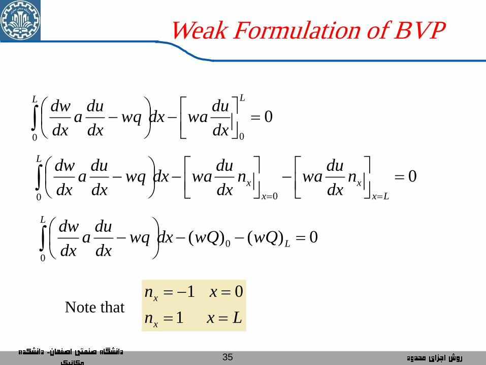
000
LL
dx
duwadxwq
dx
dua
dx
dw
000
Lx
x
x
x
L
ndx
duwan
dx
duwadxwq
dx
dua
dx
dw
0)()( 0
0
L
L
wQwQdxwqdx
dua
dx
dw
Lxn
xn
x
x
1
0 1Note that
36
Weak Formulation of BVP
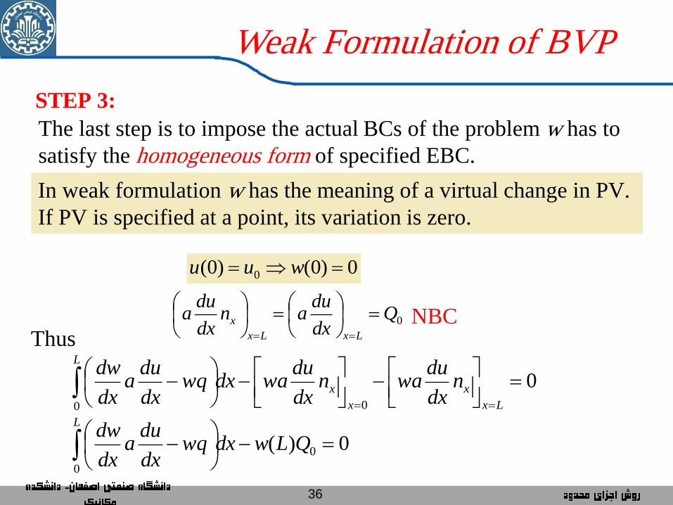
STEP 3:
The last step is to impose the actual BCs of the problem w has to
satisfy the homogeneous form of specified EBC.
In weak formulation w has the meaning of a virtual change in PV.
If PV is specified at a point, its variation is zero.
0)0()0( 0 wuu
0Qdx
duan
dx
dua
LxLx
x
NBC
000
Lx
x
x
x
L
ndx
duwan
dx
duwadxwq
dx
dua
dx
dw
Thus
0)( 0
0
QLwdxwq
dx
dua
dx
dwL
37
Linear and Bilinear Forms
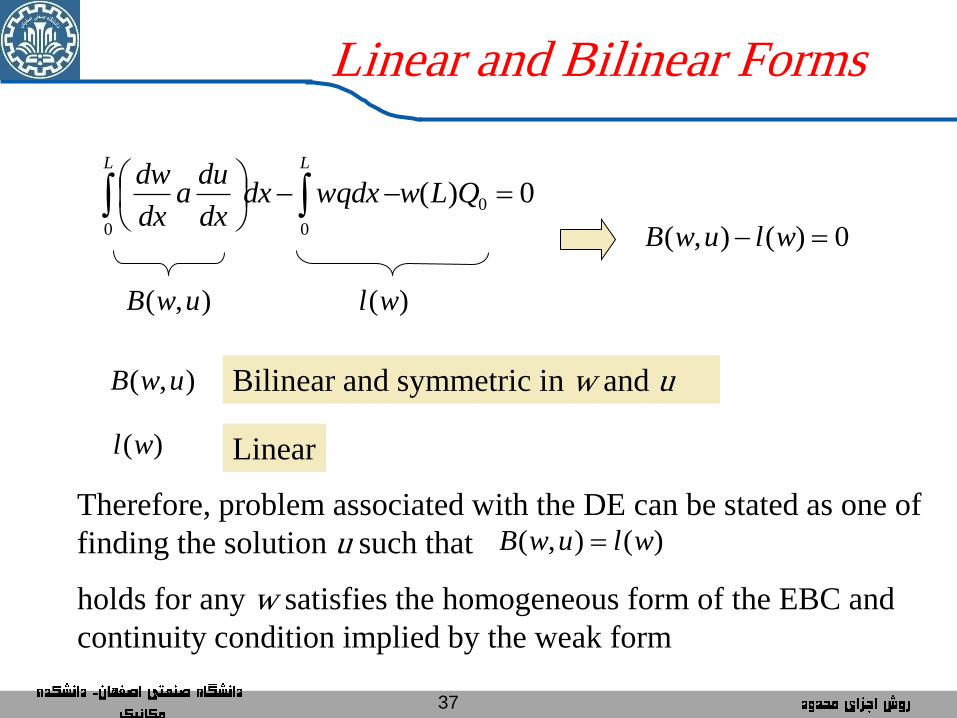
0)( 0
00
QLwwqdxdx
dx
dua
dx
dwLL
),( uwB )(wl
0)(),( wluwB
Bilinear and symmetric in w and u ),( uwB
)(wl Linear
)(),( wluwB
Therefore, problem associated with the DE can be stated as one of
finding the solution u such that
holds for any w satisfies the homogeneous form of the EBC and
continuity condition implied by the weak form
38
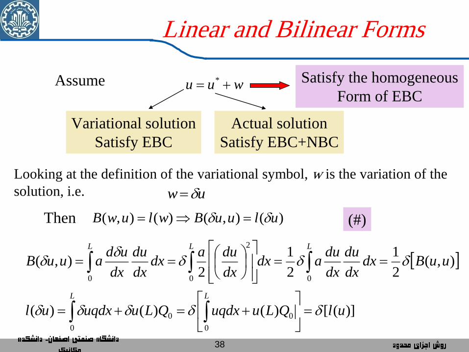
Linear and Bilinear Forms
Assume wuu *
Variational solution
Satisfy EBC
Actual solution
Satisfy EBC+NBC
Satisfy the homogeneous
Form of EBC
Looking at the definition of the variational symbol, w is the variation of the
solution, i.e. uw
Then )(),()(),( uluuBwluwB
L L
LL L
ulQLuuqdxQLuuqdxul
uuBdxdx
du
dx
duadx
dx
duadx
dx
du
dx
udauuB
0 0
00
00 0
2
)]([)()()(
),(2
1
2
1
2),(
(#)
39
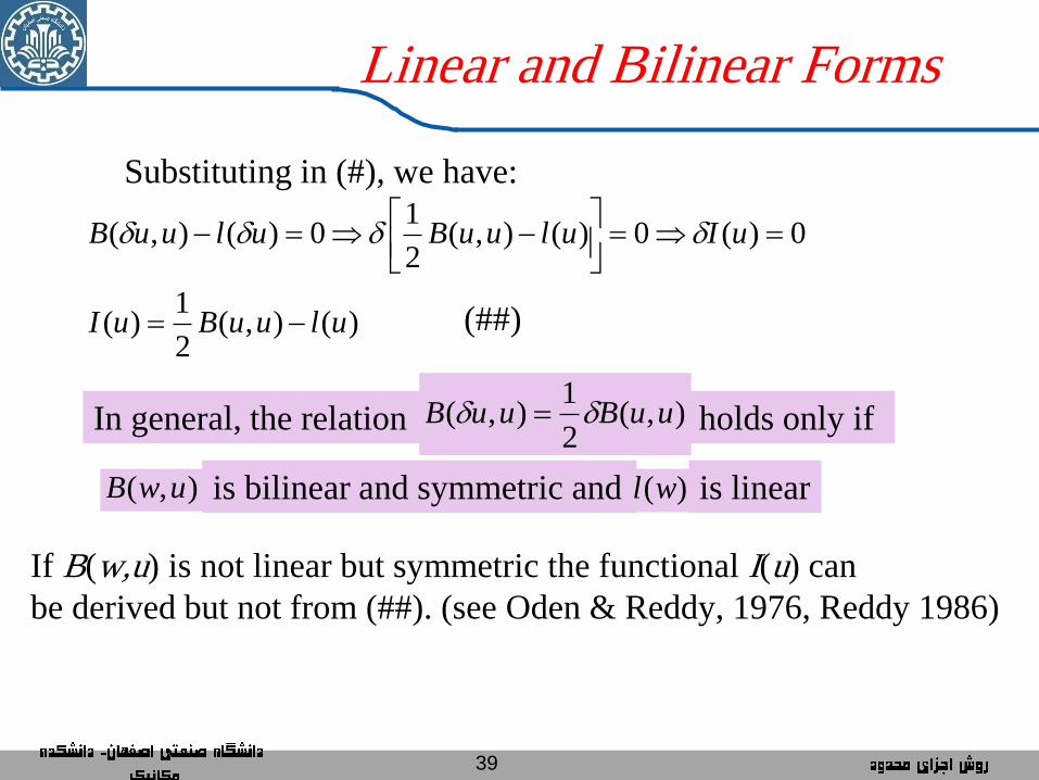
Linear and Bilinear Forms
)(),(2
1)(
0)(0)(),(2
10)(),(
uluuBuI
uIuluuBuluuB
Substituting in (#), we have:
In general, the relation ),(2
1),( uuBuuB holds only if
),( uwB is bilinear and symmetric and )(wl is linear
If B(w,u) is not linear but symmetric the functional I(u) can
be derived but not from (##). (see Oden & Reddy, 1976, Reddy 1986)
(##)
40
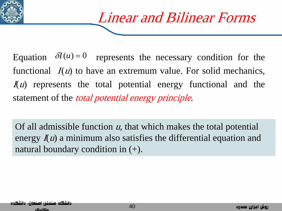
Linear and Bilinear Forms
Equation represents the necessary condition for the
functional I (u) to have an extremum value. For solid mechanics,
I(u) represents the total potential energy functional and the
statement of the total potential energy principle.
0)( uI
Of all admissible function u, that which makes the total potential
energy I(u) a minimum also satisfies the differential equation and
natural boundary condition in (+).
41
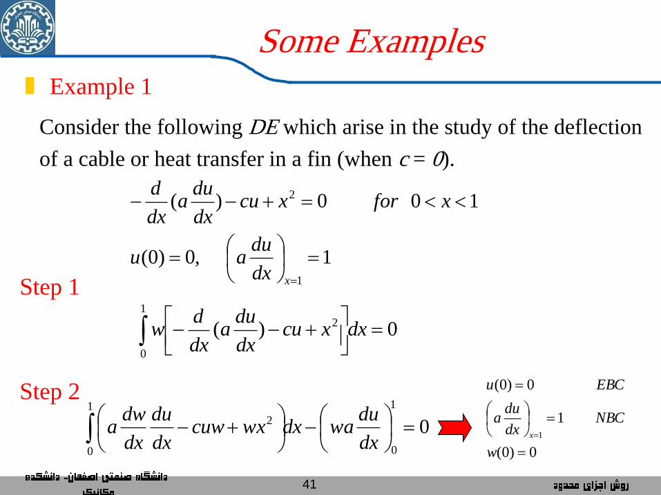
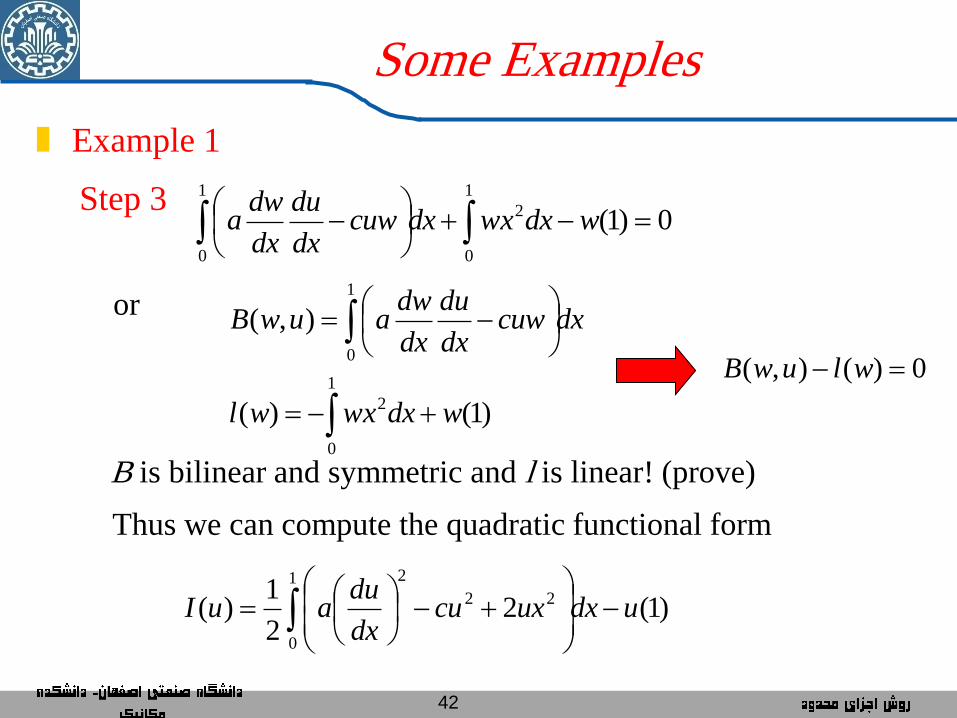
Example 1
Some Examples
Consider the following DE which arise in the study of the deflection
of a cable or heat transfer in a fin (when c = 0).
1, 0)0(
10 0)(
1
2
xdx
duau
xforxcudx
dua
dx
d
Step 1
0)(
1
0
2
dxxcu
dx
dua
dx
dw
Step 2
0
1
0
1
0
2
dx
duwadxwxcuw
dx
du
dx
dwa
0)0(
1
0)0(
1
w
NBCdx
dua
EBCu
x
42
Example 1
Some Examples
1
0
2
1
0
)1()(
),(
wdxwxwl
dxcuwdx
du
dx
dwauwB
or
0)(),( wluwB
B is bilinear and symmetric and l is linear! (prove)
Thus we can compute the quadratic functional form
0)1(
1
0
2
1
0
wdxwxdxcuw
dx
du
dx
dwa
Step 3
)1(22
1)(
1
0
22
2
udxuxcudx
duauI
43
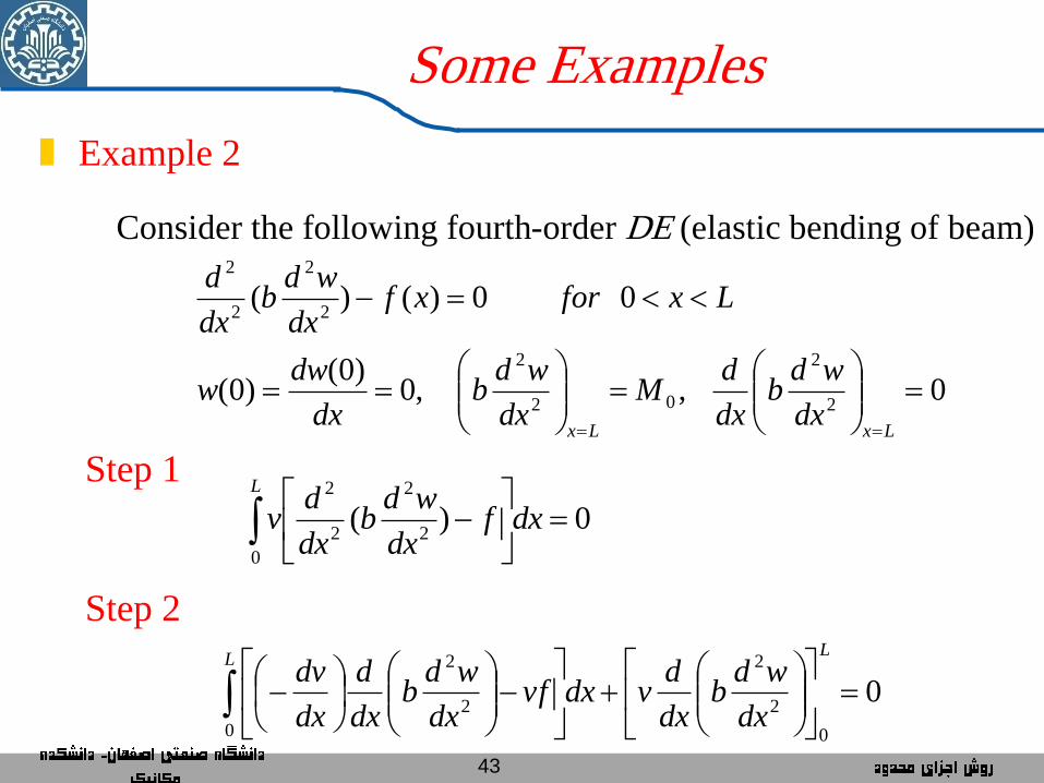
Example 2
Some Examples
Consider the following fourth-order DE (elastic bending of beam)
0, , 0)0(
)0(
0 0)()(
2
2
02
2
2
2
2
2
LxLxdx
wdb
dx
dM
dx
wdb
dx
dww
Lxforxfdx
wdb
dx
d
Step 1
0)(0
2
2
2
2
dxf
dx
wdb
dx
dv
L
Step 2
0
0
2
2
0
2
2
LL
dx
wdb
dx
dvdxvf
dx
wdb
dx
d
dx
dv
44
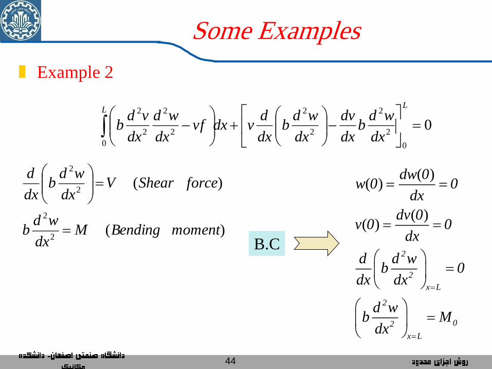
Example 2
Some Examples
0
0
2
2
2
2
0
2
2
2
2
LL
dx
wdb
dx
dv
dx
wdb
dx
dvdxvf
dx
wd
dx
vdb
) (
) (
2
2
2
2
momentBendingMdx
wdb
forceShearVdx
wdb
dx
d
( )( )
( )( )
2
2
x L
2
02
x L
dw 0w 0 0
dx
dv 0v 0 0
dx
d d wb 0
dx dx
d wb M
dx
B.C
45
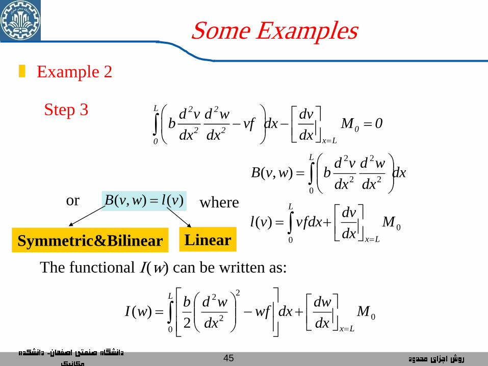
Example 2
Some Examples
L 2 2
02 2
x L0
d v d w dvb vf dx M 0
dx dx dx
Step 3
or )(),( vlwvB
0
0
0
2
2
2
2
)(
),(
Mdx
dvvfdxvl
dxdx
wd
dx
vdbwvB
Lx
L
L
where
The functional I (w) can be written as:
0
0
2
2
2
2)( M
dx
dwdxwf
dx
wdbwI
Lx
L
Symmetric&Bilinear Linear
46
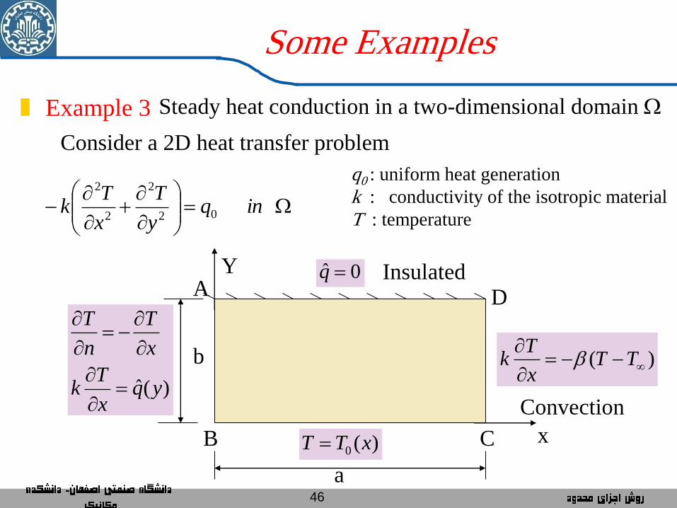
Example 3
Some Examples
Consider a 2D heat transfer problem
02
2
2
2
inqy
T
x
Tk
)(0 xTT
)(
TT
x
Tk
)(ˆ yqx
Tk
x
T
n
T
0ˆ q
Convection
B C
D A
a
b
x
Y
Steady heat conduction in a two-dimensional domain
Insulated
q0 : uniform heat generation
k : conductivity of the isotropic material
T : temperature
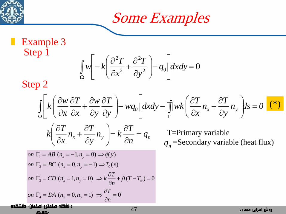
47
Example 3
Some Examples
Step 1
002
2
2
2
dxdyqy
T
x
Tkw
Step 2
0 x y
w T w T T Tk wq dxdy wk n n ds 0
x x y y x y
nyx qn
Tkn
y
Tn
x
Tk
T=Primary variable
=Secondary variable (heat flux) nq
0) 1,0 (
0)() 0,1 (
)( ) 1,0 (
)(ˆ ) 0,1 (
4
3
02
1
n
TnnDAon
TTn
TknnCDon
xTnnBCon
yqnnABon
yx
yx
yx
yx
(*)
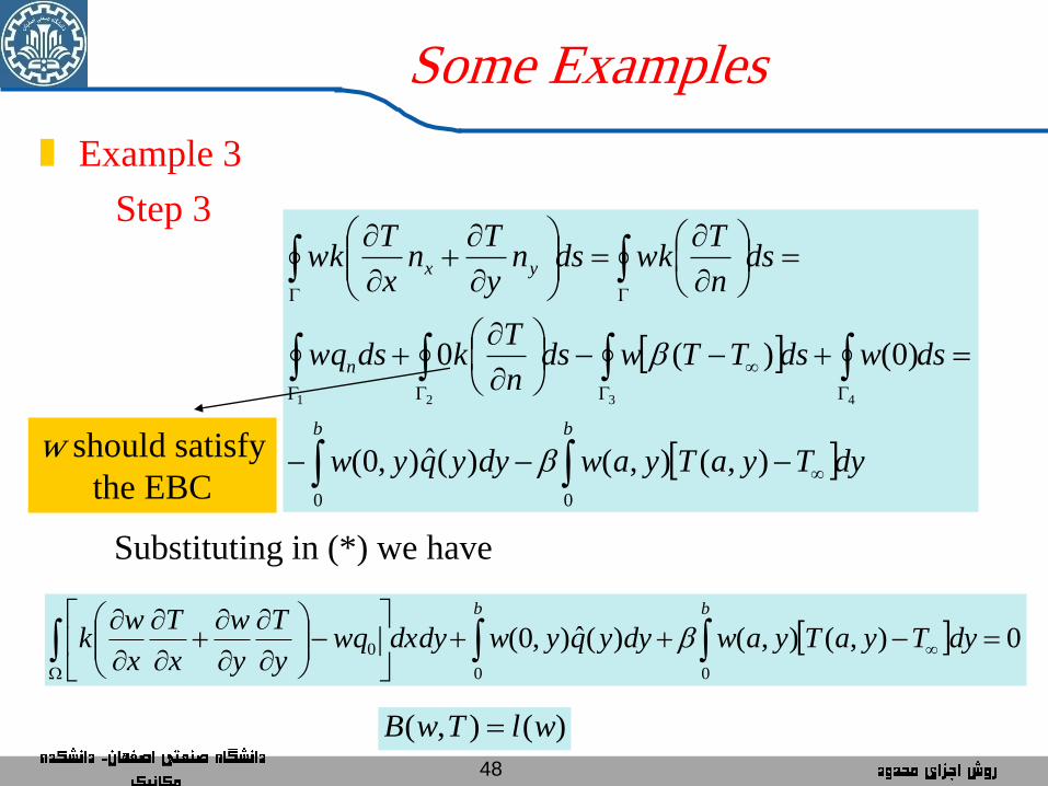
48
Example 3
Some Examples
Step 3
b b
n
yx
dyTyaTyawdyyqyw
dswdsTTwdsn
Tkdswq
dsn
Twkdsn
y
Tn
x
Twk
0 0
),(),()(ˆ),0(
)0()(0
4321
Substituting in (*) we have
0),(),()(ˆ),0(0 0
0
dyTyaTyawdyyqywdxdywqy
T
y
w
x
T
x
wk
b b
)(),( wlTwB
w should satisfy
the EBC
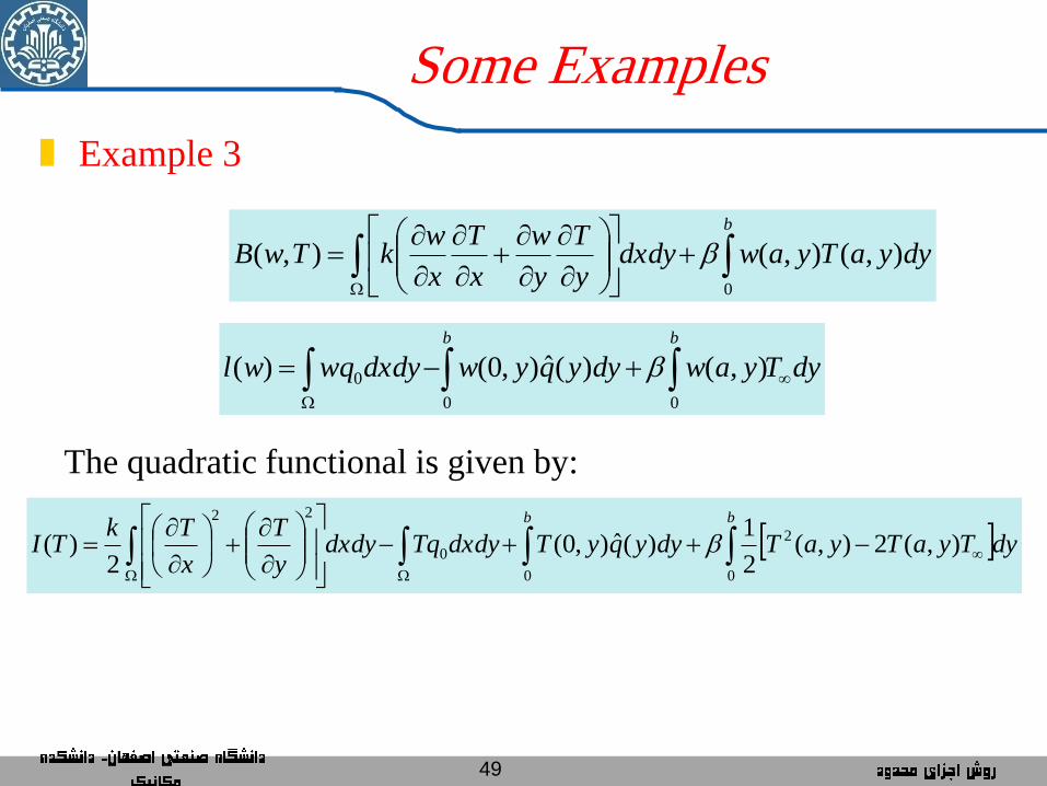
49
Example 3
Some Examples
b
dyyaTyawdxdyy
T
y
w
x
T
x
wkTwB
0
),(),(),(
dyTyawdyyqywdxdywqwl
b b
0 0
0 ),()(ˆ),0()(
The quadratic functional is given by:
b b
dyTyaTyaTdyyqyTdxdyTqdxdyy
T
x
TkTI
0 0
2
0
22
),(2),(2
1)(ˆ),0(
2)(
50
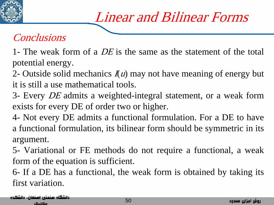
Conclusions
1- The weak form of a DE is the same as the statement of the total
potential energy.
2- Outside solid mechanics I(u) may not have meaning of energy but
it is still a use mathematical tools.
3- Every DE admits a weighted-integral statement, or a weak form
exists for every DE of order two or higher.
4- Not every DE admits a functional formulation. For a DE to have
a functional formulation, its bilinear form should be symmetric in its
argument.
5- Variational or FE methods do not require a functional, a weak
form of the equation is sufficient.
6- If a DE has a functional, the weak form is obtained by taking its
first variation.
Linear and Bilinear Forms
51
References
1- An Introduction to the Finite Element Method, by: J. N. Reddy, 3rd
ed., McGraw-Hill Education (2005). (chapter 2)
2- Energy Principles and Variational Methods in Applied Mechanics, by:
J. N. Reddy, 2nd ed., John Wiley (2002). (chapter 7)


![A Taylor-Galerkin approach for modelling a spherically ... · to the standard weighted residual integral form of the Galerkin method for the advection–dispersion equation [10,16]](https://img.pdfslide.us/doc/110x75/5ada52ab7f8b9ae1768d028a/a-taylor-galerkin-approach-for-modelling-a-spherically-the-standard-weighted.jpg)