Embed Size (px)
Citation preview
Chapter 6
Weighted Residual Methods
Weighted residual methods (WRM) assume that a solution can be approximated analytically orpiecewise analytically. In general a solution to a PDE can be expressed as a superposition of a baseset of functions
T (x, t) =
N∑
j=1
aj(t)φj(x)
where the coefficients aj are determined by a chosen method. The method attempts to minimizethe error, for instance, finite differences try to minimize the error specifically at the chosen gridpoints. WRM’s represent a particular group of methods where an integral error is minimized ina certain way and thereby defining the specific method. Depending on the maximization WRMgenerate
• the finite volume method,
• finite element methods,
• spectral methods, and also
• finite difference methods.
6.1 General Formulation
The starting point for WRM’s is an expansion in a set of base or trial functions. Often these areanalytical in which case the numerical solution will be analytical
T (x, y, z, t) = T0(x, y, z, t) +N∑
j=1
aj(t)φj(x, y, z) (6.1)
81
CHAPTER 6. WEIGHTED RESIDUAL METHODS 82
with the trial functions φj(x, y, z). T0(x, y, z, t) is chosen to satisfy initial or boundary conditionsand the coefficients aj(t) have to be determined. possible trial functions are
φj(x) = xj−1 or φj(x) = sin(jπx).
The expansion is chosen to satisfy a differential equation L(T ) = 0 (where T is the exact solution),e.g.,
L(T ) =∂T
∂t− α
∂2T
∂x2= 0
However, the numerical solution is an approximate solution, i.e., T 6= T such that the operator Lapplied to T produces a residual
L(T ) = R
The goal of WRM’s is to choose the coefficients aj such that the residual R becomes small (in fact0) over a chosen domain. In integral form this can be achieved with the condition
∫ ∫ ∫Wm(x, y, z)Rdxdydz = 0 (6.2)
where Wm is a set of weight functions (m = 1, ...M) which are used to evaluate (6.2). The exactsolution always satisfies (6.2) if the weight functions are analytic. This is in particular true also forany given subdomain of the domain for which a solution is sought.
There are four main categories of weight or test functions which are applied in WRM’s.
i) Subdomain method: Here the domain is divided in M subdomains Dm where
Wm =
{1 in Dm
0 outside(6.3)
such that this method minimizes the residual error in each of the chosen subdomains. Note that thechoice of the subdomains is free. In many cases an equal division of the total domain is likely thebest choice. However, if higher resolution (and a corresponding smaller error) in a particular areais desired, a non-uniform choice may be more appropriate.
ii) Collocation method: In this method the weight functions are chosen to be Dirac delta func-tions
Wm(x) = δ(x − xm) (6.4)
such that the error is zero at the chosen nodes xm.
CHAPTER 6. WEIGHTED RESIDUAL METHODS 83
iii) Least squares method: This method uses derivatives of the residual itself as weight functionsin the form
Wm(x) =∂R
∂am
. (6.5)
The motivation for this choice is to minimize∫ ∫ ∫
R2dxdydz of the computational domain. Notethat this choice of the weight function implies
∂
∂am
∫ ∫ ∫R2dxdydz = 0
for all values of am.
iv) Galerkin method: In this method the weight functions are chosen to be identical to the basefunctions.
Wm(x) = φm(x)
In particular if the base function set is orthogonal (∫
φm(x)φn(x) = 0 if m 6= n), this choice ofweight functions implies that the residual R is rendered orthogonal with the condition (6.2) for allbase functions.
Note that M weight functions yield M conditions (or equations) from which to determine the Ncoefficients aj . To determine these N coefficients uniquely we need N independent condition(equations).
Example: Consider the ordinary differential equation
dy
dx− y = 0 (6.6)
for 0 ≤ x ≤ 1 with y(0) = 1. Let us assume an approximate solution in the form of polynomials
y = 1 +N∑
j=1
ajxj (6.7)
where the constant 1 satisfies the boundary condition. Substituting this expression into the differ-ential equation (6.6) gives the residual
R = −1 +N∑
j=1
aj
(jxj−1 − xj
)(6.8)
We can now compute the coefficients aj with the various methods.
CHAPTER 6. WEIGHTED RESIDUAL METHODS 84
Galerkin method:
Here we use the weight functions Wm = xm−1. The maximization implies with (6.2)
∫ 1
0
xm−1
[−1 +
N∑
j=1
aj
(jxj−1 − xj
)]
dx = 0
or
−
∫ 1
0
xm−1dx +N∑
j=1
[aj
(j
∫ 1
0
xm−1xj−1dx −
∫ 1
0
xm−1xjdx
)]= 0
which yields after integration
−1
m+
N∑
j=1
aj
[j
m + j − 1−
1
m + j
]= 0 (6.9)
With the matrix S (with elements smj = jm+j−1
− 1m+j
) and the vector D (with the elementsdm = − 1
m) we can rewrite (6.9) as
SA = D (6.10)
The solution A of this set of equations requires to invert S. For N = 3 the system becomes
1/2 2/3 3/41/6 5/12 11/201/12 3/10 13/30
a1
a2
a3
=
1
1/21/3
For this set the approximate solution becomes
y = 1 + 1.0141x + 0.4225x2 + 0.2817x3
Least squares method:
Here the weight functions are
Wm(x) =∂R
∂am= mxm−1 − xm
This gives the residual condition
∫ 1
0
(mxm−1 − xm
)[−1 +
N∑
j=1
aj
(jxj−1 − xj
)]
dx =
−1 +1
m + 1+
N∑
j=1
[aj
∫ 1
0
(mxm−1 − xm
) (jxj−1 − xj
)dx
]= 0
CHAPTER 6. WEIGHTED RESIDUAL METHODS 85
or
−1 +1
m + 1+
N∑
j=1
aj
[jm
m + j − 1−
j + m
m + j+
1
m + j + 1
]= 0
Subdomain method:
Weight functions:
Wm =
{1 x ∈ (m−1
N, m
N]
0 outside
Condition for the residual error:
∫ mN
m−1
N
[−1 +
N∑
j=1
aj
(jxj−1 − xj
)]
dx = 0
Collocation method:
Collocation point (for the Dirac delta function): xm = m−1N
.
Condition for the residual error:
∫ 1
0
δ(x − xm)
[−1 +
N∑
j=1
aj
(jxj−1 − xj
)]
dx = 0
6.2 Finite Volume Method
This section illustrate the use of the finite volume method first for a PDE involving first orderderivatives and later for second order derivatives. The program FIVOL will be introduced whichcan be used to solve Laplace’s equation or Poisson’s equation, i.e, equations of the elliptic type.
6.2.1 First order derivatives
Let us consider the equation∂q
∂t+
∂F
∂x+
∂G
∂y= 0 (6.11)
which is to be solved with the subdomain method on a domain given by coordinate line (j, k)describing a curved coordinate system. This equation is a typical continuity equation like theequations for conservation of mass, momentum etc.
CHAPTER 6. WEIGHTED RESIDUAL METHODS 86
k-1
k
k+1
j-1
j
j+1
A
B
C
D
x
y
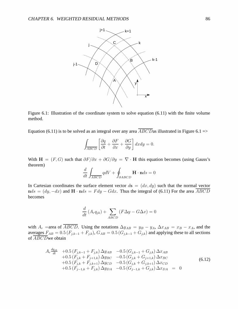
Figure 6.1: Illustration of the coordinate system to solve equation (6.11) with the finite volumemethod.
Equation (6.11) is to be solved as an integral over any area ABCDas illustrated in Figure 6.1 =>∫
ABCD
[∂q
∂t+
∂F
∂x+
∂G
∂y
]dxdy = 0.
With H = (F, G) such that ∂F/∂x + ∂G/∂y = ∇ · H this equation becomes (using Gauss’stheorem)
d
dt
∫
ABCD
qdV +
∮
∂ABCD
H · nds = 0
In Cartesian coordinates the surface element vector ds = (dx, dy) such that the normal vectornds = (dy,−dx) and H · nds = Fdy − Gdx. Thus the integral of (6.11) For the area ABCDbecomes
d
dt(Arqjk) +
∑
ABCD
(F∆y − G∆x) = 0
with Ar =area of ABCD. Using the notations ∆yAB = yB − yA, ∆xAB = xB − xA, and theaverages FAB = 0.5 (Fj,k−1 + Fj,k), GAB = 0.5 (Gj,k−1 + Gj,k) and applying these to all sectionsof ABCDwe obtain
Ardqjk
dt+0.5 (Fj,k−1 + Fj,k)∆yAB −0.5 (Gj,k−1 + Gj,k) ∆xAB
+0.5 (Fj,k + Fj+1,k)∆yBC −0.5 (Gj,k + Gj+1,k) ∆xBC
+0.5 (Fj,k + Fj,k+1) ∆yCD −0.5 (Gj,k + Gj,k+1)∆xCD
+0.5 (Fj−1,k + Fj,k) ∆yDA −0.5 (Gj−1,k + Gj,k)∆xDA = 0
(6.12)
CHAPTER 6. WEIGHTED RESIDUAL METHODS 87
In case of a uniform grid parallel to the x, and the y axes the area is Ar = ∆x∆y and equation(6.12) reduces to
dqjk
dt+
Fj+1,k − Fj−1,k
2∆x+
Gj+1,k − Gj−1,k
2∆y= 0
where the spatial derivative is equal to that for the centered space finite difference approximation.
6.2.2 Second order derivatives
To introduce the finite volume second derivatives let us consider Laplace’s equation
∂2φ
∂x2+
∂2φ
∂x2= 0 (6.13)
k-1
k
k+1
j-1
j
j+1
A
B
C
D
x
y
A’
B’
C’
D’
x
y
XW
Y
Z
rWZ
rXY
(A)
(B)
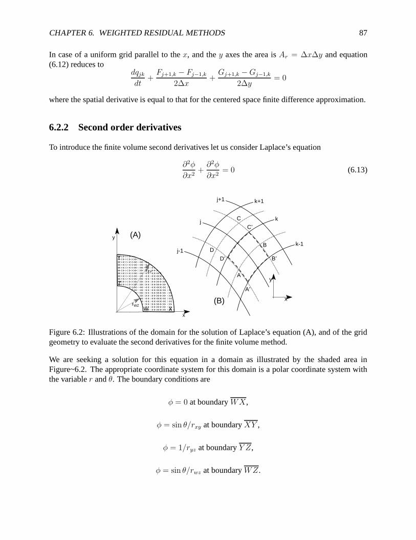
Figure 6.2: Illustrations of the domain for the solution of Laplace’s equation (A), and of the gridgeometry to evaluate the second derivatives for the finite volume method.
We are seeking a solution for this equation in a domain as illustrated by the shaded area inFigure~6.2. The appropriate coordinate system for this domain is a polar coordinate system withthe variable r and θ. The boundary conditions are
φ = 0 at boundary WX,
φ = sin θ/rxy at boundary XY ,
φ = 1/ryz at boundary Y Z,
φ = sin θ/rwz at boundary WZ.
CHAPTER 6. WEIGHTED RESIDUAL METHODS 88
With this choice of boundary conditions Laplace’s equation (6.13) has the exact solution
φ =sin θ
r
To apply the finite volume method we determine the integral of the residual in the area given byABCD in Figure 6.2
∫ ∫
ABCD
(∂2φ
∂x2+
∂2φ
∂y2
)dxdy =
∮
∂ABCD
H · nds = 0 (6.14)
with H · nds = ∂φ∂x
dy − ∂φ∂y
dx. Note that H = (∂φ/∂x, ∂φ/∂y) and that the direction normal tods = (dx, dy) is nds = (dy,−dx). Using the geometry shown in Figure 6.2 equation (6.14) isapproximated with
∂φ
∂x
∣∣∣∣j,k−1/2
∆yAB −∂φ
∂y
∣∣∣∣j,k−1/2
∆xAB
+∂φ
∂x
∣∣∣∣j+1,k
∆yBC −∂φ
∂y
∣∣∣∣j+1,k
∆xBC
+∂φ
∂x
∣∣∣∣j,k+1/2
∆yCD −∂φ
∂y
∣∣∣∣j,k+1/2
∆xCD
+∂φ
∂x
∣∣∣∣j−1,k
∆yDA −∂φ
∂y
∣∣∣∣j−1,k
∆xDA = 0 (6.15)
The derivatives ∂φ/∂x and ∂φ/∂y at the midpoints of each section AB, BC, etc are determinedthrough averages over the appropriate section. For instance along AB the derivatives are
∂φ
∂x
∣∣∣∣j,k−1/2
=1
SAB
∫ ∫
A′B′C′D′
∂φ
∂xdxdy =
1
SAB
∮
∂A′B′C′D′
φdy
∂φ
∂y
∣∣∣∣j,k−1/2
=1
SAB
∫ ∫
A′B′C′D′
∂φ
∂ydxdy = −
1
SAB
∮
∂A′B′C′D′
φdx
with SAB as the area of A′B′C ′D′ and∮
∂A′B′C′D′
φdy = φj,k−1∆yA′B′ + φB∆yB′C′ + φj,k∆yC′D′ + φA∆yD′A′
∮
∂A′B′C′D′
φdx = φj,k−1∆xA′B′ + φB∆xB′C′ + φj,k∆xC′D′ + φA∆xD′A′
If the mesh is not too distorted we can approximate
∆yA′B′ ≈ −∆yC′D′ ≈ ∆yAB
∆yB′C′ ≈ −∆yD′A′ ≈ ∆yk−1,k
CHAPTER 6. WEIGHTED RESIDUAL METHODS 89
���
���
���
���
∆ � �−∆ � �� ������
�����
�
∆ � �
∆ � �� ������
�
�
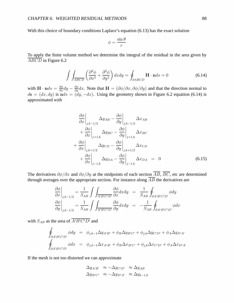
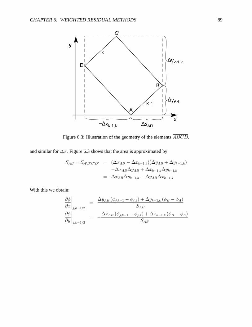
Figure 6.3: Illustration of the geometry of the elements ABCD.
and similar for ∆x. Figure 6.3 shows that the area is approximated by
SAB = SA′B′C′D′ = (∆xAB − ∆xk−1,k)(∆yAB + ∆yk−1,k)
−∆xAB∆yAB + ∆xk−1,k∆yk−1,k
= ∆xAB∆yk−1,k − ∆yAB∆xk−1,k
With this we obtain:
∂φ
∂x
∣∣∣∣j,k−1/2
=∆yAB (φj,k−1 − φj,k) + ∆yk−1,k (φB − φA)
SAB
∂φ
∂y
∣∣∣∣j,k−1/2
= −∆xAB (φj,k−1 − φj,k) + ∆xk−1,k (φB − φA)
SAB
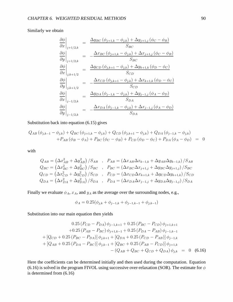
CHAPTER 6. WEIGHTED RESIDUAL METHODS 90
Similarly we obtain
∂φ
∂x
∣∣∣∣j+1/2,k
=∆yBC (φj+1,k − φj,k) + ∆yj+1,j (φC − φB)
SBC
∂φ
∂y
∣∣∣∣j+1/2,k
= −∆xBC (φj+1,k − φj,k) + ∆xj+1,j (φC − φB)
SBC
∂φ
∂x
∣∣∣∣j,k+1/2
=∆yCD (φj,k+1 − φj,k) + ∆yk+1,k (φD − φC)
SCD
∂φ
∂y
∣∣∣∣j,k+1/2
= −∆xCD (φj,k+1 − φj,k) + ∆xk+1,k (φD − φC)
SCD
∂φ
∂x
∣∣∣∣j−1/2,k
=∆yDA (φj−1,k − φj,k) + ∆yj−1,j (φA − φD)
SDA
∂φ
∂y
∣∣∣∣j−1/2,k
= −∆xDA (φj−1,k − φj,k) + ∆xj−1,j (φA − φD)
SDA
Substitution back into equation (6.15) gives
QAB (φj,k−1 − φj,k) + QBC (φj+1,k − φj,k) + QCD (φj,k+1 − φj,k) + QDA (φj−1,k − φj,k)
+PAB (φB − φA) + PBC (φC − φB) + PCD (φD − φC) + PDA (φA − φD) = 0
with
QAB =(∆x2
AB + ∆y2AB
)/SAB , PAB = (∆xAB∆xk−1,k + ∆yAB∆yk−1,k) /SAB
QBC =(∆x2
BC + ∆y2BC
)/SBC , PBC = (∆xBC∆xj+1,j + ∆yBC∆yj+1,j) /SBC
QCD =(∆x2
CD + ∆y2CD
)/SCD , PCD = (∆xCD∆xk+1,k + ∆yCD∆yk+1,k) /SCD
QDA =(∆x2
DA + ∆y2DA
)/SDA , PDA = (∆xDA∆xj−1,j + ∆yDA∆yj−1,j) /SDA
Finally we evaluate φA, xA, and yA as the average over the surrounding nodes, e.g.,
φA = 0.25(φj,k + φj−1,k + φj−1,k−1 + φj,k−1)
Substitution into our main equation then yields
0.25 (PCD − PDA)φj−1,k+1 + 0.25 (PBC − PCD) φj+1,k+1
+0.25 (PAB − PBC) φj+1,k−1 + 0.25 (PDA − PAB) φj−1,k−1
+ [QCD + 0.25 (PBC − PDA)]φj,k+1 + [QDA + 0.25 (PCD − PAB)] φj−1,k
+ [QAB + 0.25 (PDA − PBC)] φj,k−1 + [QBC + 0.25 (PAB − PCD)] φj+1,k
− (QAB + QBC + QCD + QDA)φj,k = 0 (6.16)
Here the coefficients can be determined initially and then used during the computation. Equation(6.16) is solved in the program FIVOL using successive over-relaxation (SOR). The estimate for φis determined from (6.16)
CHAPTER 6. WEIGHTED RESIDUAL METHODS 91
φ?j,k = {0.25 (PCD − PDA) φj−1,k+1 + 0.25 (PBC − PCD)φj+1,k+1 (6.17)
+0.25 (PAB − PBC) φj+1,k−1 + 0.25 (PDA − PAB)φj−1,k−1
+ [QCD + 0.25 (PBC − PDA)] φj,k+1 + [QDA + 0.25 (PCD − PAB)]φj−1,k
+ [QAB + 0.25 (PDA − PBC)] φj,k−1 + [QBC + 0.25 (PAB − PCD)] φj+1,k}n
/ (QAB + QBC + QCD + QDA)
The iteration step is completed with
φn+1j,k = φn
j,k + ω(φ?j,k − φn
j,k) (6.18)
Note that the discretized equation (6.16) reduces to centered finite differences on a uniform rect-angular grid
φj−1,k − 2φj,k + φj+1,k
∆x2+
φj,k−1 − 2φj,k + φj,k+1
∆y2= 0 (6.19)
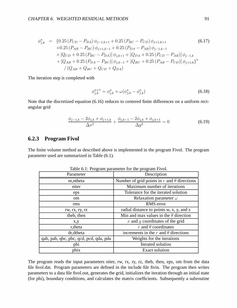
6.2.3 Program Fivol
The finite volume method as described above is implemented in the program Fivol. The programparameter used are summarized in Table (6.1).
Table 6.1: Program parameter for the program Fivol.Parameter Description
nr,ntheta Number of grid points in r and θ directionsniter Maximum number of iterationseps Tolerance for the iterated solutionom Relaxation parameter ωrms RMS error
rw, rx, ry, rz radial distance to points w, x, y, and ztheb, then Min and max values in the θ direction
x,y x and y coordinates of the gridr,theta r and θ coordinates
dr,dtheta increments in the r and θ directionsqab, pab, qbc, pbc, qcd, pcd, qda, pda Weights for the iterations
phi Iterated solutionphix Exact solution
The program reads the input parameters niter, rw, rx, ry, rz, theb, then, eps, om from the datafile fivol.dat. Program parameters are defined in the include file fivin. The program then writesparameters to a data file fivol.out, generates the grid, initializes the iteration through an initial state(for phi), boundary conditions, and calculates the matrix coefficients. Subsequently a subroutine
CHAPTER 6. WEIGHTED RESIDUAL METHODS 92
SOR is called until the iterated solution tolerance is reached. The result is written to a binary filewhich can serve as input for the plotting routine plofivol.
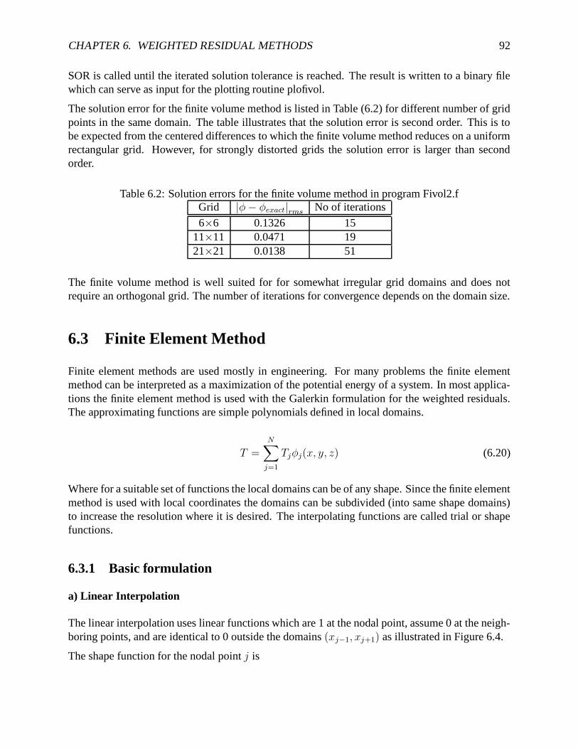
The solution error for the finite volume method is listed in Table (6.2) for different number of gridpoints in the same domain. The table illustrates that the solution error is second order. This is tobe expected from the centered differences to which the finite volume method reduces on a uniformrectangular grid. However, for strongly distorted grids the solution error is larger than secondorder.
Table 6.2: Solution errors for the finite volume method in program Fivol2.fGrid |φ − φexact|rms No of iterations
6×6 0.1326 1511×11 0.0471 1921×21 0.0138 51
The finite volume method is well suited for for somewhat irregular grid domains and does notrequire an orthogonal grid. The number of iterations for convergence depends on the domain size.
6.3 Finite Element Method
Finite element methods are used mostly in engineering. For many problems the finite elementmethod can be interpreted as a maximization of the potential energy of a system. In most applica-tions the finite element method is used with the Galerkin formulation for the weighted residuals.The approximating functions are simple polynomials defined in local domains.
T =N∑
j=1
Tjφj(x, y, z) (6.20)
Where for a suitable set of functions the local domains can be of any shape. Since the finite elementmethod is used with local coordinates the domains can be subdivided (into same shape domains)to increase the resolution where it is desired. The interpolating functions are called trial or shapefunctions.
6.3.1 Basic formulation
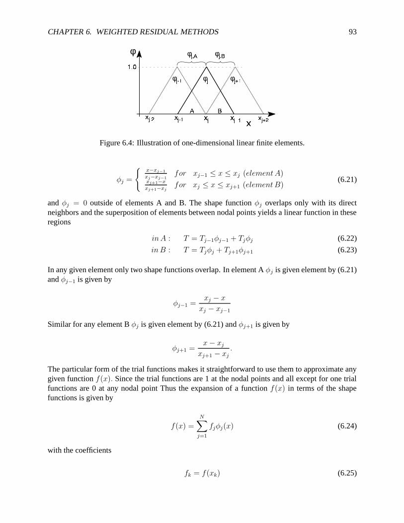
a) Linear Interpolation
The linear interpolation uses linear functions which are 1 at the nodal point, assume 0 at the neigh-boring points, and are identical to 0 outside the domains (xj−1, xj+1) as illustrated in Figure 6.4.
The shape function for the nodal point j is
CHAPTER 6. WEIGHTED RESIDUAL METHODS 93
� �� � ��� �
� �φ φ� � � φ� � �
� � � � ���
φ�
� � ��� � � ���
φ� ��� φ� ���
Figure 6.4: Illustration of one-dimensional linear finite elements.
φj =
{x−xj−1
xj−xj−1for xj−1 ≤ x ≤ xj (element A)
xj+1−x
xj+1−xjfor xj ≤ x ≤ xj+1 (element B)
(6.21)
and φj = 0 outside of elements A and B. The shape function φj overlaps only with its directneighbors and the superposition of elements between nodal points yields a linear function in theseregions
in A : T = Tj−1φj−1 + Tjφj (6.22)
in B : T = Tjφj + Tj+1φj+1 (6.23)
In any given element only two shape functions overlap. In element A φj is given element by (6.21)and φj−1 is given by
φj−1 =xj − x
xj − xj−1
Similar for any element B φj is given element by (6.21) and φj+1 is given by
φj+1 =x − xj
xj+1 − xj
.
The particular form of the trial functions makes it straightforward to use them to approximate anygiven function f(x). Since the trial functions are 1 at the nodal points and all except for one trialfunctions are 0 at any nodal point Thus the expansion of a function f(x) in terms of the shapefunctions is given by
f(x) =
N∑
j=1
fjφj(x) (6.24)
with the coefficients
fk = f(xk) (6.25)
CHAPTER 6. WEIGHTED RESIDUAL METHODS 94
where the xk are the nodal points. Formally this is seen by f(xk) =∑N
j=1 fjφj(xk) = fk
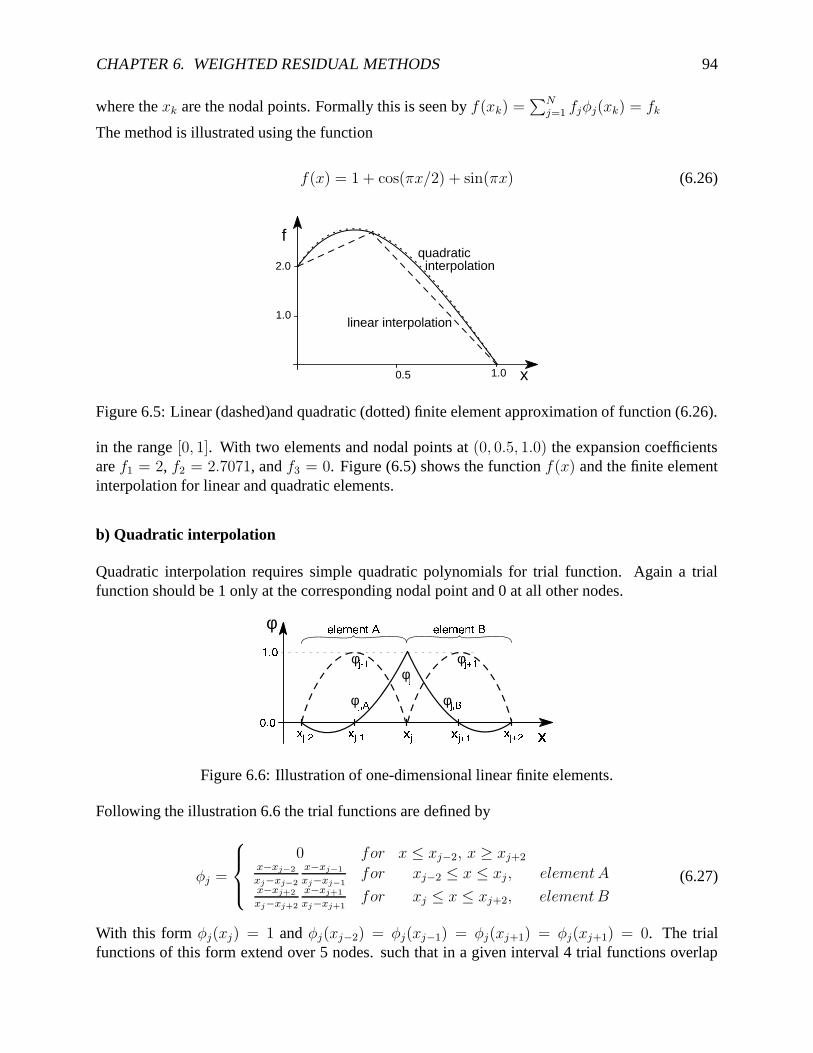
The method is illustrated using the function
f(x) = 1 + cos(πx/2) + sin(πx) (6.26)
f
x
2.0
1.0
0.5 1.0
quadratic interpolation
linear interpolation
Figure 6.5: Linear (dashed)and quadratic (dotted) finite element approximation of function (6.26).
in the range [0, 1]. With two elements and nodal points at (0, 0.5, 1.0) the expansion coefficientsare f1 = 2, f2 = 2.7071, and f3 = 0. Figure (6.5) shows the function f(x) and the finite elementinterpolation for linear and quadratic elements.
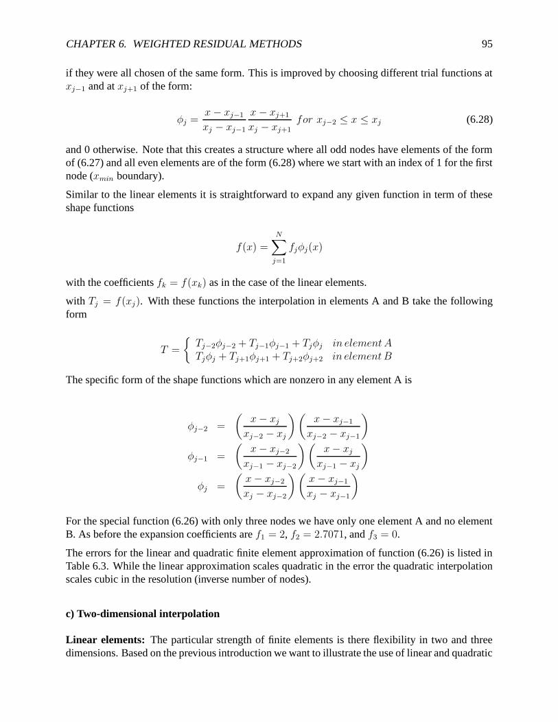
b) Quadratic interpolation
Quadratic interpolation requires simple quadratic polynomials for trial function. Again a trialfunction should be 1 only at the corresponding nodal point and 0 at all other nodes.
��� ����������
� �� �
��� �φ
φ� � � φ� � �
� � � � ��
φ�
� � � � ���
��� �����������
φ� �� φ� ��
��� �
Figure 6.6: Illustration of one-dimensional linear finite elements.
Following the illustration 6.6 the trial functions are defined by
φj =
0 for x ≤ xj−2, x ≥ xj+2x−xj−2
xj−xj−2
x−xj−1
xj−xj−1for xj−2 ≤ x ≤ xj, element A
x−xj+2
xj−xj+2
x−xj+1
xj−xj+1for xj ≤ x ≤ xj+2, element B
(6.27)
With this form φj(xj) = 1 and φj(xj−2) = φj(xj−1) = φj(xj+1) = φj(xj+1) = 0. The trialfunctions of this form extend over 5 nodes. such that in a given interval 4 trial functions overlap
CHAPTER 6. WEIGHTED RESIDUAL METHODS 95
if they were all chosen of the same form. This is improved by choosing different trial functions atxj−1 and at xj+1 of the form:
φj =x − xj−1
xj − xj−1
x − xj+1
xj − xj+1for xj−2 ≤ x ≤ xj (6.28)
and 0 otherwise. Note that this creates a structure where all odd nodes have elements of the formof (6.27) and all even elements are of the form (6.28) where we start with an index of 1 for the firstnode (xmin boundary).
Similar to the linear elements it is straightforward to expand any given function in term of theseshape functions
f(x) =N∑
j=1
fjφj(x)
with the coefficients fk = f(xk) as in the case of the linear elements.
with Tj = f(xj). With these functions the interpolation in elements A and B take the followingform
T =
{Tj−2φj−2 + Tj−1φj−1 + Tjφj in element ATjφj + Tj+1φj+1 + Tj+2φj+2 in element B
The specific form of the shape functions which are nonzero in any element A is
φj−2 =
(x − xj
xj−2 − xj
)(x − xj−1
xj−2 − xj−1
)
φj−1 =
(x − xj−2
xj−1 − xj−2
)(x − xj
xj−1 − xj
)
φj =
(x − xj−2
xj − xj−2
)(x − xj−1
xj − xj−1
)
For the special function (6.26) with only three nodes we have only one element A and no elementB. As before the expansion coefficients are f1 = 2, f2 = 2.7071, and f3 = 0.
The errors for the linear and quadratic finite element approximation of function (6.26) is listed inTable 6.3. While the linear approximation scales quadratic in the error the quadratic interpolationscales cubic in the resolution (inverse number of nodes).
c) Two-dimensional interpolation
Linear elements: The particular strength of finite elements is there flexibility in two and threedimensions. Based on the previous introduction we want to illustrate the use of linear and quadratic
CHAPTER 6. WEIGHTED RESIDUAL METHODS 96
Table 6.3: Error for linear and quadratic finite element interpolation for the function in (6.26).
Linear Interpolation Quadratic interpolationNo of elements RMS error No of elements RMS error
2 0.18662 1 0.040284 0.04786 2 0.015996 0.02138 3 0.004848 0.01204 4 0.00206
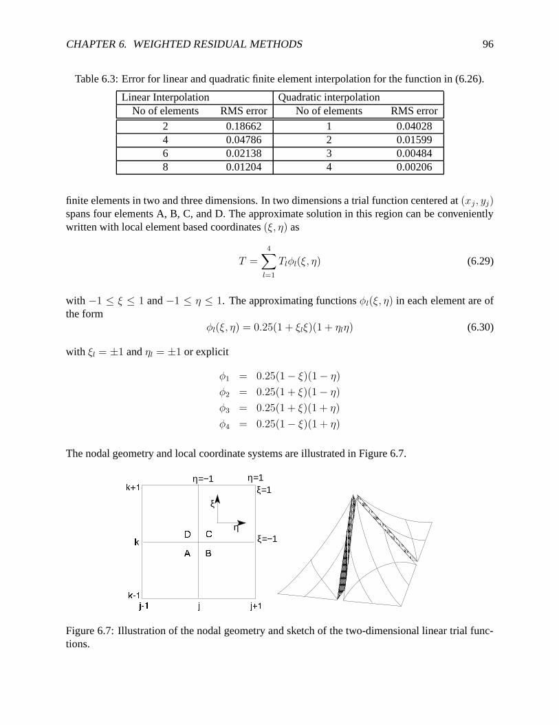
finite elements in two and three dimensions. In two dimensions a trial function centered at (xj, yj)spans four elements A, B, C, and D. The approximate solution in this region can be convenientlywritten with local element based coordinates (ξ, η) as
T =
4∑
l=1
Tlφl(ξ, η) (6.29)
with −1 ≤ ξ ≤ 1 and −1 ≤ η ≤ 1. The approximating functions φl(ξ, η) in each element are ofthe form
φl(ξ, η) = 0.25(1 + ξlξ)(1 + ηlη) (6.30)
with ξl = ±1 and ηl = ±1 or explicit
φ1 = 0.25(1 − ξ)(1 − η)
φ2 = 0.25(1 + ξ)(1 − η)
φ3 = 0.25(1 + ξ)(1 + η)
φ4 = 0.25(1 − ξ)(1 + η)
The nodal geometry and local coordinate systems are illustrated in Figure 6.7.
ξ
η
η=−1 η=1
ξ=−1
ξ=1
� �
��
� �������
�
�����
�����
Figure 6.7: Illustration of the nodal geometry and sketch of the two-dimensional linear trial func-tions.
CHAPTER 6. WEIGHTED RESIDUAL METHODS 97
A solution is constructed separate in each element A, B, C, and D where continuity is provided bythe overlapping shape functions. For instance a solution in element A implies that shape functionswith values of 1 along the boundary to element B overlap into the region of element B and similarfor all other boundaries of element A.
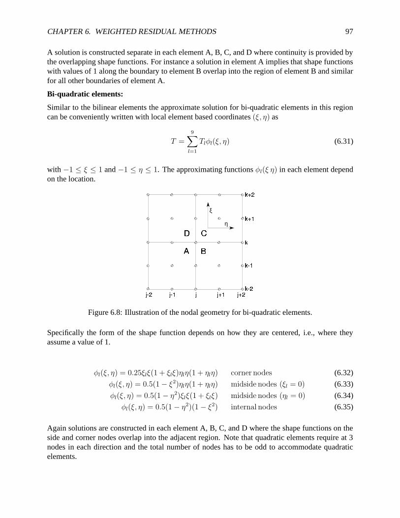
Bi-quadratic elements:
Similar to the bilinear elements the approximate solution for bi-quadratic elements in this regioncan be conveniently written with local element based coordinates (ξ, η) as
T =
9∑
l=1
Tlφl(ξ, η) (6.31)
with −1 ≤ ξ ≤ 1 and −1 ≤ η ≤ 1. The approximating functions φl(ξ η) in each element dependon the location.
� �
��
�����
ξ
η
���
�
��� �
����
�������� � ��� � ����
Figure 6.8: Illustration of the nodal geometry for bi-quadratic elements.
Specifically the form of the shape function depends on how they are centered, i.e., where theyassume a value of 1.
φl(ξ, η) = 0.25ξlξ(1 + ξlξ)ηlη(1 + ηlη) corner nodes (6.32)
φl(ξ, η) = 0.5(1 − ξ2)ηlη(1 + ηlη) midside nodes (ξl = 0) (6.33)
φl(ξ, η) = 0.5(1 − η2)ξlξ(1 + ξlξ) midside nodes (ηl = 0) (6.34)
φl(ξ, η) = 0.5(1 − η2)(1 − ξ2) internal nodes (6.35)
Again solutions are constructed in each element A, B, C, and D where the shape functions on theside and corner nodes overlap into the adjacent region. Note that quadratic elements require at 3nodes in each direction and the total number of nodes has to be odd to accommodate quadraticelements.
CHAPTER 6. WEIGHTED RESIDUAL METHODS 98
6.3.2 Finite element method applied to the Sturm-Liouville equation
Here we will use the Galerkin finite element method to discretize and solve the Sturm-Liouvilleequation
d2y
dx2+ y = F (x) (6.36)
subject to boundary conditions y(0) = 0 and dy/dx(1) = 0 and
F (x) = −L∑
l=1
al sin ((l − 0.5)πx) . (6.37)
The exact solution to this problem for F (x) is given by
y(x) = −
L∑
l=1
al
1 − ((l − 0.5)π)2 sin ((l − 0.5)πx) . (6.38)
The trial solution is as before
y =
N∑
j=1
yjφj.
Linear Interpolation:
In an element based coordinate system we use local coordinates with
φj = 0.5(1 + ξ) and ξ =2
“x−
xj−1+xj
2
”
∆xjfor element A
φj = 0.5(1 − ξ) and ξ =2
“x−
xj+xj+1
2
”
∆xj+1for element B
with ∆xj = xj − xj−1, and ∆xj+1 = xj+1 − xj . The residual is
R =d2y
dx2+ y − F (x)
and the weight function for the weighted residual is wm = φm which yields the equation
∫ 1
0
φm(x)
(d2y
dx2+ y − F (x)
)dx = 0
One can integrate the first term brackets by parts
∫ 1
0
φmd2y
dx2dx =
[φm
dy
dx
]1
0
−
∫ 1
0
dφm
dx
dy
dxdx
CHAPTER 6. WEIGHTED RESIDUAL METHODS 99
because the boundary conditions imply φ1 = 0 and dy/dx(1) = 0 such that[φm
deydx
]10
= 0 such
that the residual equation becomesN∑
j=1
[yj
∫ 1
0
(−
dφm
dx
dφj
dx+ φmφj
)dx
]=
∫ 1
0
φmF (x)dx
or in matrix formBY = G
with the elements
bmj =
∫ 1
0
(−
dφm
dx
dφj
dx+ φmφj
)dx
gm =
∫ 1
0
φmF (x)dx.
In the computation of these elements it is convenient to make use of the local coordinates. Itshould also be noted that the residual equation only has contributions for j = m − 1, j = m, andm = j + 1. With the transformation to local coordinates we have in element A
d
dx=
dξ
dx
d
dξ=
2
∆xj
d
dξ
dx =dx
dξdξ =
∆xj
2dξ
and in element B
d
dx=
dξ
dx
d
dξ=
2
∆xj+1
d
dξ
dx =dx
dξdξ =
∆xj+1
2dξ
with ∆xj = xj − xj−1 and ∆xj+1 = xj+1 − xj.
Element bm,m−1: A contribution exists only in region A for node m (corresponding to a region Bfor node m − 1). Thus
bm,m−1 =
∫ 1
0
(−
dφm
dx
dφm−1
dx+ φmφm−1
)dx
=
∫ 1
−1
(−
dξA
dx
dφA
dξ
dφB
dξ+
dx
dξAφAφB
)dξ
=1
2∆xm
∫ 1
−1
dξ +∆xm
8
∫ 1
−1
(1 − ξ2)dξ
=1
∆xm+
∆xm
6
CHAPTER 6. WEIGHTED RESIDUAL METHODS 100
Similar the element bm,m+1 involves only overlap in region B of element φm with region A ofelement φm+1. The expression is the same only that it regards the interval ∆xm+1. Thus
bm,m+1 =1
∆xm+1+
∆xm+1
6
Element bm,m: Here we have overlap of φm with itself in regions A and B:
bm,m =
∫ 1
0
(−
dφm
dx
dφm
dx+ φmφm
)dx
=
∫ 1
−1
(−
dξ
dx
(dφA
dξ
)2
+dx
dξφ2
A
)
A
dξ +
∫ 1
−1
(−
dξ
dx
(dφB
dξ
)2
+dx
dξφ2
B
)
B
dξ
=
∫ 1
−1
(−
2
∆xm
(1
2
)2
+∆xm
2
(1 + ξ
2
)2)
A
dξ
+
∫ 1
−1
(−
2
∆xm+1
(1
2
)2
+∆xm+1
2
(1 − ξ
2
)2)
A
dξ
= −1
∆xm
−1
∆xm+1
+∆xm
8
∫ 1
−1
(1 + ξ)2dξ +∆xm+1
8
∫ 1
−1
(1 − ξ)2dξ
= −1
∆xm−
1
∆xm+1+
∆xm + ∆xm+1
3
In summary the nonzero elements bmj for 2 ≤ m ≤ N − 1 are
bm,m−1 =1
∆xm+
∆xm
6
bm,m = −
[1
∆xm+
1
∆xm+1
]+
∆xm + ∆xm+1
3
bm,m+1 =1
∆xm+1+
∆xm+1
6
for m = N
bN,N−1 =1
∆xN+
∆xN
6
bN,N = −1
∆xN+
∆xN
6bN,N+1 = 0.
CHAPTER 6. WEIGHTED RESIDUAL METHODS 101
The inhomogeneity F (x) is known analytically such that one can evaluate∫ 1
0φmF (x)dx directly.
However, in more complex situations it is more convenient to interpolate F (x) through the trialfunctions
F (x) =
N∑
j=1
Fjφj.
such that
gm =
N∑
j=1
Fj
∫ 1
0
φmφjdx
For the linear interpolation this yields
gm =∆xm
6Fm−1 +
∆xm + ∆xm+1
3Fm +
∆xm+1
6Fm+1
Finally consider the special case of a uniform grid with ∆xm = ∆xm+1 = ∆x. In this case theequation for the coefficients becomes
ym−1 − 2ym + ym+1
∆x2+
(1
6ym−1 +
2
3ym +
1
6ym+1
)=
(1
6Fm−1 +
2
3Fm +
1
6Fm+1
)
Exercise: Determine the elements at the min and max boundary, i.e., b1,1, b1,2, and b2,1.
Elements with m = 1 (y1 = 0): There is no equation for y1 needed because y1 = 0 such that theindices for the array dimensions decrease by 1.
Elements with m = 2
y2
∫ 1
0
(−
dφ2
dx
dφ2
dx+ φ2φ2
)dx + y3
∫ 1
0
(−
dφ2
dx
dφ3
dx+ φ2φ3
)dx =
∫ 1
0
φ2F (x)dx
Elements with m = N
yN−1
∫ 1
0
(−
dφN
dx
dφN−1
dx+ φNφN−1
)dx + yN
∫ 1
0
(−
dφN
dx
dφN
dx+ φNφN
)dx =
∫ 1
0
φNF (x)dx
Quadratic interpolation:
The program offers the possibility to use a linear or quadratic finite element interpolation. For thesecond case the equations for the bmj are
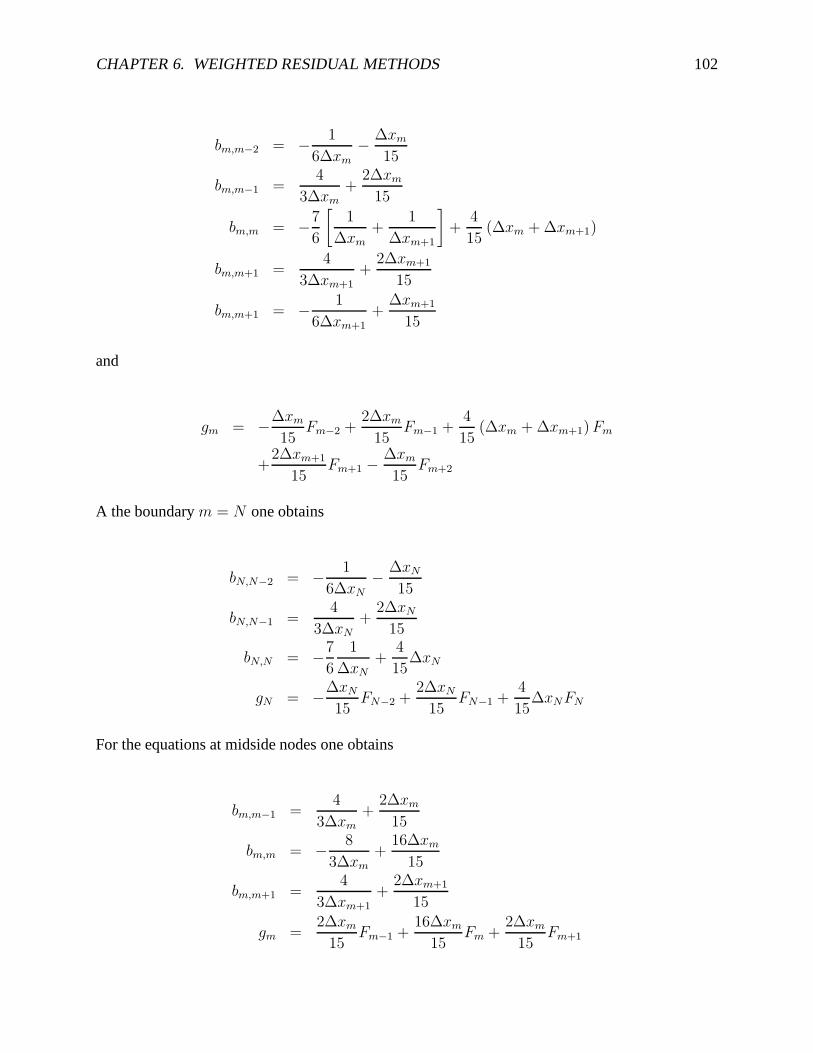
CHAPTER 6. WEIGHTED RESIDUAL METHODS 102
bm,m−2 = −1
6∆xm−
∆xm
15
bm,m−1 =4
3∆xm+
2∆xm
15
bm,m = −7
6
[1
∆xm+
1
∆xm+1
]+
4
15(∆xm + ∆xm+1)
bm,m+1 =4
3∆xm+1
+2∆xm+1
15
bm,m+1 = −1
6∆xm+1
+∆xm+1
15
and
gm = −∆xm
15Fm−2 +
2∆xm
15Fm−1 +
4
15(∆xm + ∆xm+1) Fm
+2∆xm+1
15Fm+1 −
∆xm
15Fm+2
A the boundary m = N one obtains
bN,N−2 = −1
6∆xN−
∆xN
15
bN,N−1 =4
3∆xN+
2∆xN
15
bN,N = −7
6
1
∆xN+
4
15∆xN
gN = −∆xN
15FN−2 +
2∆xN
15FN−1 +
4
15∆xNFN
For the equations at midside nodes one obtains
bm,m−1 =4
3∆xm
+2∆xm
15
bm,m = −8
3∆xm
+16∆xm
15
bm,m+1 =4
3∆xm+1
+2∆xm+1
15
gm =2∆xm
15Fm−1 +
16∆xm
15Fm +
2∆xm
15Fm+1
CHAPTER 6. WEIGHTED RESIDUAL METHODS 103
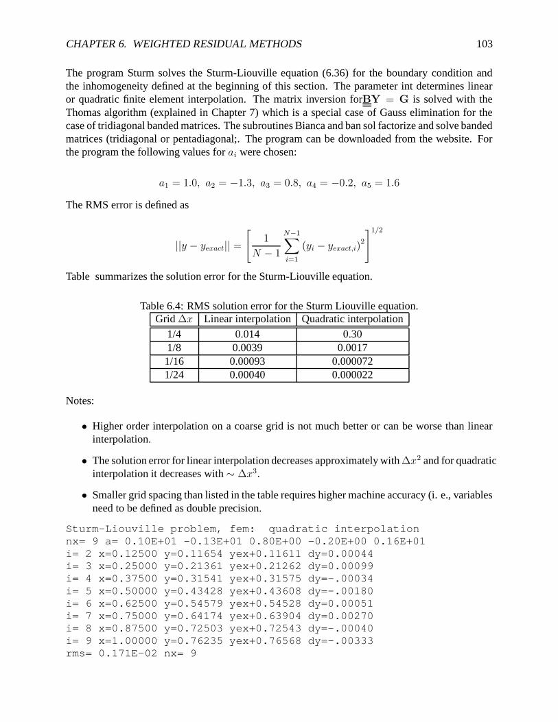
The program Sturm solves the Sturm-Liouville equation (6.36) for the boundary condition andthe inhomogeneity defined at the beginning of this section. The parameter int determines linearor quadratic finite element interpolation. The matrix inversion forBY = G is solved with theThomas algorithm (explained in Chapter 7) which is a special case of Gauss elimination for thecase of tridiagonal banded matrices. The subroutines Bianca and ban sol factorize and solve bandedmatrices (tridiagonal or pentadiagonal;. The program can be downloaded from the website. Forthe program the following values for ai were chosen:
a1 = 1.0, a2 = −1.3, a3 = 0.8, a4 = −0.2, a5 = 1.6
The RMS error is defined as
||y − yexact|| =
[1
N − 1
N−1∑
i=1
(yi − yexact,i)2
]1/2
Table summarizes the solution error for the Sturm-Liouville equation.
Table 6.4: RMS solution error for the Sturm Liouville equation.Grid ∆x Linear interpolation Quadratic interpolation
1/4 0.014 0.301/8 0.0039 0.0017
1/16 0.00093 0.0000721/24 0.00040 0.000022
Notes:
• Higher order interpolation on a coarse grid is not much better or can be worse than linearinterpolation.
• The solution error for linear interpolation decreases approximately with ∆x2 and for quadraticinterpolation it decreases with ∼ ∆x3.
• Smaller grid spacing than listed in the table requires higher machine accuracy (i. e., variablesneed to be defined as double precision.
Sturm-Liouville problem, fem: quadratic interpolationnx= 9 a= 0.10E+01 -0.13E+01 0.80E+00 -0.20E+00 0.16E+01i= 2 x=0.12500 y=0.11654 yex+0.11611 dy=0.00044i= 3 x=0.25000 y=0.21361 yex+0.21262 dy=0.00099i= 4 x=0.37500 y=0.31541 yex+0.31575 dy=-.00034i= 5 x=0.50000 y=0.43428 yex+0.43608 dy=-.00180i= 6 x=0.62500 y=0.54579 yex+0.54528 dy=0.00051i= 7 x=0.75000 y=0.64174 yex+0.63904 dy=0.00270i= 8 x=0.87500 y=0.72503 yex+0.72543 dy=-.00040i= 9 x=1.00000 y=0.76235 yex+0.76568 dy=-.00333rms= 0.171E-02 nx= 9
CHAPTER 6. WEIGHTED RESIDUAL METHODS 104
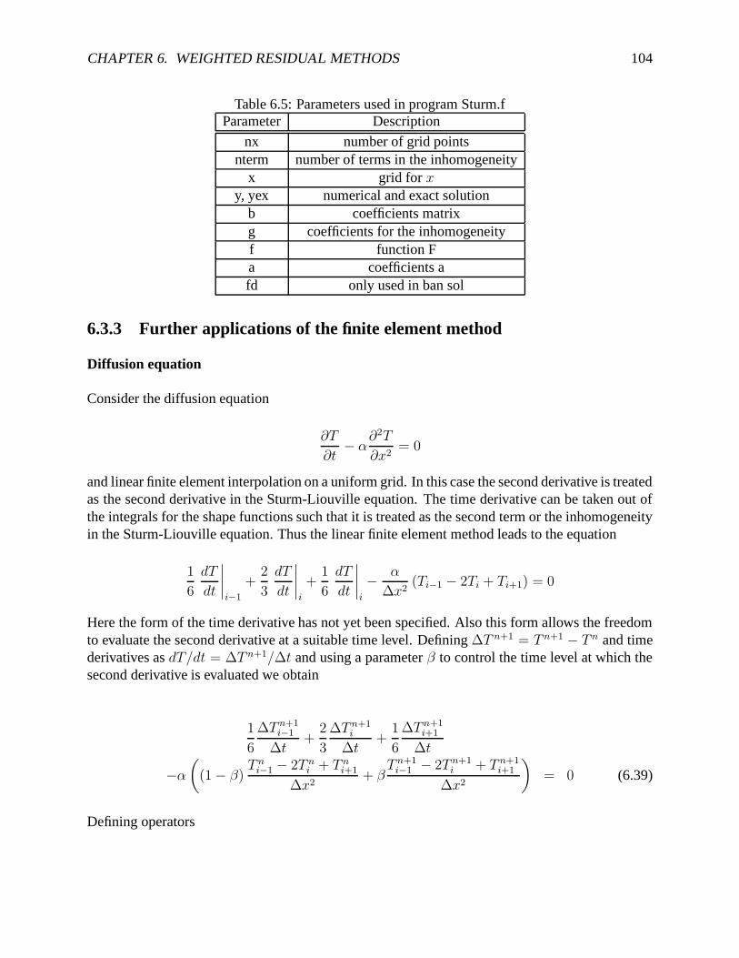
Table 6.5: Parameters used in program Sturm.fParameter Description
nx number of grid pointsnterm number of terms in the inhomogeneity
x grid for xy, yex numerical and exact solution
b coefficients matrixg coefficients for the inhomogeneityf function Fa coefficients afd only used in ban sol
6.3.3 Further applications of the finite element method
Diffusion equation
Consider the diffusion equation
∂T
∂t− α
∂2T
∂x2= 0
and linear finite element interpolation on a uniform grid. In this case the second derivative is treatedas the second derivative in the Sturm-Liouville equation. The time derivative can be taken out ofthe integrals for the shape functions such that it is treated as the second term or the inhomogeneityin the Sturm-Liouville equation. Thus the linear finite element method leads to the equation
1
6
dT
dt
∣∣∣∣i−1
+2
3
dT
dt
∣∣∣∣i
+1
6
dT
dt
∣∣∣∣i
−α
∆x2(Ti−1 − 2Ti + Ti+1) = 0
Here the form of the time derivative has not yet been specified. Also this form allows the freedomto evaluate the second derivative at a suitable time level. Defining ∆T n+1 = T n+1 − T n and timederivatives as dT/dt = ∆T n+1/∆t and using a parameter β to control the time level at which thesecond derivative is evaluated we obtain
1
6
∆T n+1i−1
∆t+
2
3
∆T n+1i
∆t+
1
6
∆T n+1i+1
∆t
−α
((1 − β)
T ni−1 − 2T n
i + T ni+1
∆x2+ β
T n+1i−1 − 2T n+1
i + T n+1i+1
∆x2
)= 0 (6.39)
Defining operators
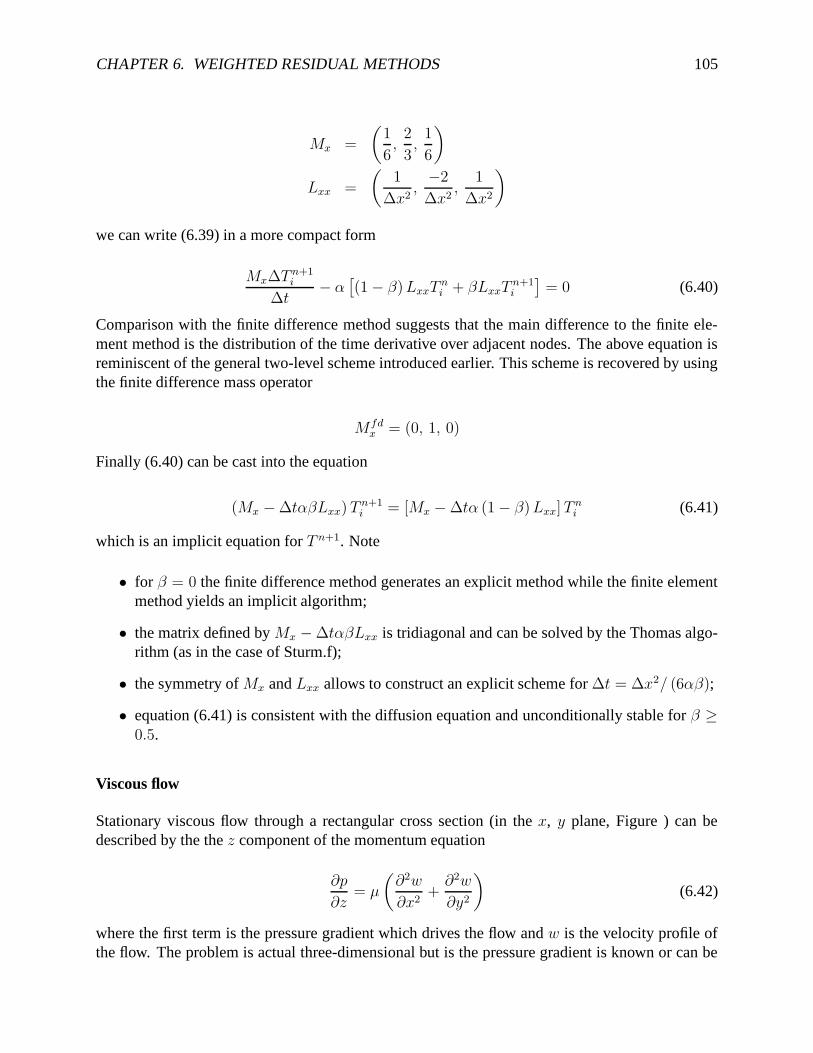
CHAPTER 6. WEIGHTED RESIDUAL METHODS 105
Mx =
(1
6,
2
3,
1
6
)
Lxx =
(1
∆x2,−2
∆x2,
1
∆x2
)
we can write (6.39) in a more compact form
Mx∆T n+1i
∆t− α
[(1 − β)LxxT
ni + βLxxT
n+1i
]= 0 (6.40)
Comparison with the finite difference method suggests that the main difference to the finite ele-ment method is the distribution of the time derivative over adjacent nodes. The above equation isreminiscent of the general two-level scheme introduced earlier. This scheme is recovered by usingthe finite difference mass operator
Mfdx = (0, 1, 0)
Finally (6.40) can be cast into the equation
(Mx − ∆tαβLxx) T n+1i = [Mx − ∆tα (1 − β)Lxx] T
ni (6.41)
which is an implicit equation for T n+1. Note
• for β = 0 the finite difference method generates an explicit method while the finite elementmethod yields an implicit algorithm;
• the matrix defined by Mx − ∆tαβLxx is tridiagonal and can be solved by the Thomas algo-rithm (as in the case of Sturm.f);
• the symmetry of Mx and Lxx allows to construct an explicit scheme for ∆t = ∆x2/ (6αβ);
• equation (6.41) is consistent with the diffusion equation and unconditionally stable for β ≥0.5.
Viscous flow
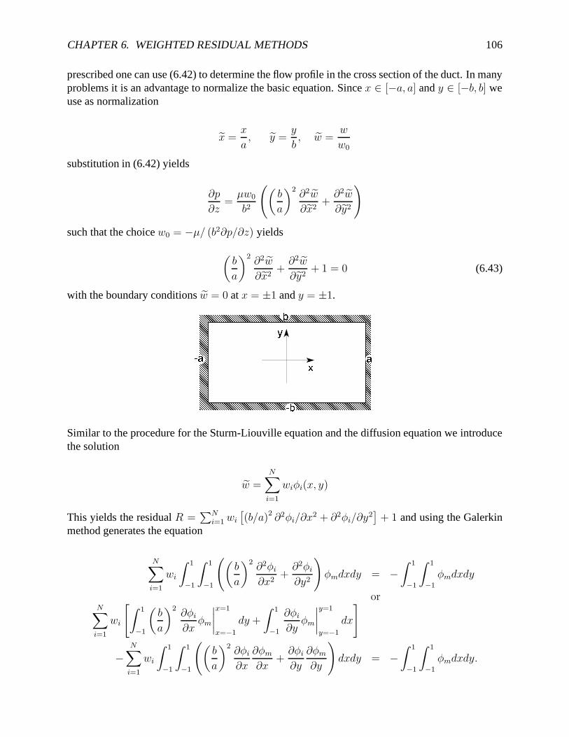
Stationary viscous flow through a rectangular cross section (in the x, y plane, Figure ) can bedescribed by the the z component of the momentum equation
∂p
∂z= µ
(∂2w
∂x2+
∂2w
∂y2
)(6.42)
where the first term is the pressure gradient which drives the flow and w is the velocity profile ofthe flow. The problem is actual three-dimensional but is the pressure gradient is known or can be
CHAPTER 6. WEIGHTED RESIDUAL METHODS 106
prescribed one can use (6.42) to determine the flow profile in the cross section of the duct. In manyproblems it is an advantage to normalize the basic equation. Since x ∈ [−a, a] and y ∈ [−b, b] weuse as normalization
x =x
a, y =
y
b, w =
w
w0
substitution in (6.42) yields
∂p
∂z=
µw0
b2
((b
a
)2∂2w
∂x2+
∂2w
∂y2
)
such that the choice w0 = −µ/ (b2∂p/∂z) yields
(b
a
)2∂2w
∂x2+
∂2w
∂y2+ 1 = 0 (6.43)
with the boundary conditions w = 0 at x = ±1 and y = ±1.�
��
�� �
�
�
Similar to the procedure for the Sturm-Liouville equation and the diffusion equation we introducethe solution
w =
N∑
i=1
wiφi(x, y)
This yields the residual R =∑N
i=1 wi
[(b/a)2 ∂2φi/∂x2 + ∂2φi/∂y2
]+ 1 and using the Galerkin
method generates the equation
N∑
i=1
wi
∫ 1
−1
∫ 1
−1
((b
a
)2∂2φi
∂x2+
∂2φi
∂y2
)φmdxdy = −
∫ 1
−1
∫ 1
−1
φmdxdy
orN∑
i=1
wi
[∫ 1
−1
(b
a
)2∂φi
∂xφm
∣∣∣∣x=1
x=−1
dy +
∫ 1
−1
∂φi
∂yφm
∣∣∣∣y=1
y=−1
dx
]
−
N∑
i=1
wi
∫ 1
−1
∫ 1
−1
((b
a
)2∂φi
∂x
∂φm
∂x+
∂φi
∂y
∂φm
∂y
)dxdy = −
∫ 1
−1
∫ 1
−1
φmdxdy.
CHAPTER 6. WEIGHTED RESIDUAL METHODS 107
For the chosen boundary conditions the first two integral are zero such that the resulting equationcan be written as
BW = G (6.44)
with
bmi = −
∫ 1
−1
∫ 1
−1
((b
a
)2∂φi
∂x
∂φm
∂x+
∂φi
∂y
∂φm
∂y
)dxdy (6.45)
gm =
∫ 1
−1
∫ 1
−1
φmdxdy (6.46)
In the following we replace the single index i with a pair k, l representing the x and y coordinates.The indices k and l range from 2 to nx−1 and from 2 to ny−1 respectively because the boundarycondition imply that the coefficient of the shape function at the boundaries is zero. The x integra-tion of the first term in (6.45) yields the operator Lxx and the y integration of this term yield theoperator My with
Lxxwk,l =wk−1,l − 2wk,l + wk+1,l
∆x2(6.47)
Mywk,l =1
6wk,l−1 +
2
3wk,l +
1
6wk,l+1 (6.48)
such that equation (6.44) assumes the form
[(b
a
)2
My ⊗ Lxx + Mx ⊗ Lyy
]wk,l = −1 (6.49)
with
My ⊗ Lxxwk,l =1
6
[wk−1,l−1 − 2wk,l−1 + wk+1,l−1
∆x2
]+
2
3
[wk−1,l − 2wk,l + wk+1,l
∆x2
]
+1
6
[wk−1,l+1 − 2wk,l+1 + wk+1,l+1
∆x2
](6.50)
Mx ⊗ Lyywk,l =1
6
[wk−1,l−1 − 2wk−1,l + wk−1,l+1
∆y2
]+
2
3
[wk,l−1 − 2wk,l + wk,l+1
∆y2
]
+1
6
[wk+1,l−1 − 2wk+1,l + wk+1,l+1
∆y2
](6.51)
and similar for Mx⊗Lyywk,l. In a corresponding finite difference approach we would have Mx,fd =(0, 1, 0).
Notes:
CHAPTER 6. WEIGHTED RESIDUAL METHODS 108
• The operator Lxx and My are commutative. The result does not depend on the order theintegration in (6.47) is executed.
• The method provides a straightforward way to employ finite element methods similar tofinite difference methods.
The result provides a simple equation which can be used with SOR to solve the coefficients for theshape functions. Solving equation (6.49) for wk,l yields
w∗
k,l =3
4c0[1. + c1 (wk−1,l−1 + wk+1,l−1 + wk−1,l+1 + wk+1,l+1)
+ c2 (wk−1,l + wk+1,l) + c3 (wk,l−1 + wk,l+1)]
with
c0 =
(b
a
)21
∆x2+
1
∆y2
c1 =1
6c0
c2 =
(b
a
)22
3∆x2−
1
3∆y2
c3 = −
(b
a
)21
3∆x2+
2
3∆y2
With the usual SOR method the solution is iterated using
wn+1k,l = wn
k,l + λ(w∗
k,l − wnk,l
)
The program duct.f can be found on the course web page. To provide a reference for the approxi-mate solution the exact solution is given by
w =
(8
π2
)2 N∑
i=1,3,5..
N∑
j=1,3,5..
(−1)(i+j)/2−1
ij[(
iba
)2+ j2
] cos
(iπx
2
)cos
(jπy
2
)
A second important measure for this problem is the total flow rate q, i.e., the flow integrated overthe cross sectional area
q = 2
(8
π2
)3 N∑
i=1,3,5..
N∑
j=1,3,5..
1
i2j2[(
iba
)2+ j2
]
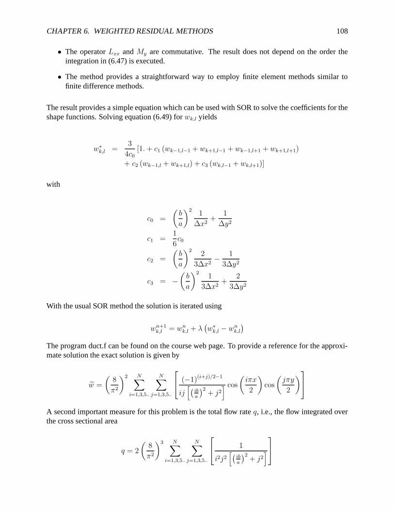
CHAPTER 6. WEIGHTED RESIDUAL METHODS 109
Table 6.6: Input parameters for the program duct.fVariable Value Description
me 2 method: 1-linear elements, 2-3pt cent dif:nem 25 no terms in exact solutionipr 1 ipr=0, prints solutions to the output file duct.out
niter 800 max no iterations for SORbar 1.0e-0 aspect ratio a/b for channeleps .1e-5 tolerance par for SORom 1.5e0 relaxation parameter (SOR), λ
The structure is similar to that of Fivol.f. The program package uses an include file ductin whichdeclares all variables and common blocks and it make use of a parameter file duct.dat. Variablesdeclared in the parameter file are summarized in Table 6.6.
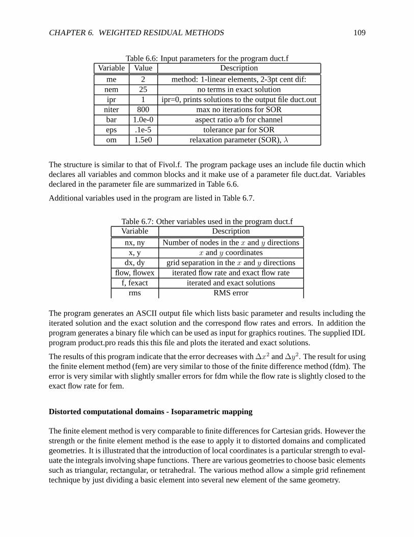
Additional variables used in the program are listed in Table 6.7.
Table 6.7: Other variables used in the program duct.fVariable Description
nx, ny Number of nodes in the x and y directionsx, y x and y coordinates
dx, dy grid separation in the x and y directionsflow, flowex iterated flow rate and exact flow rate
f, fexact iterated and exact solutionsrms RMS error
The program generates an ASCII output file which lists basic parameter and results including theiterated solution and the exact solution and the correspond flow rates and errors. In addition theprogram generates a binary file which can be used as input for graphics routines. The supplied IDLprogram product.pro reads this this file and plots the iterated and exact solutions.
The results of this program indicate that the error decreases with ∆x2 and ∆y2. The result for usingthe finite element method (fem) are very similar to those of the finite difference method (fdm). Theerror is very similar with slightly smaller errors for fdm while the flow rate is slightly closed to theexact flow rate for fem.
Distorted computational domains - Isoparametric mapping
The finite element method is very comparable to finite differences for Cartesian grids. However thestrength or the finite element method is the ease to apply it to distorted domains and complicatedgeometries. It is illustrated that the introduction of local coordinates is a particular strength to eval-uate the integrals involving shape functions. There are various geometries to choose basic elementssuch as triangular, rectangular, or tetrahedral. The various method allow a simple grid refinementtechnique by just dividing a basic element into several new element of the same geometry.
CHAPTER 6. WEIGHTED RESIDUAL METHODS 110
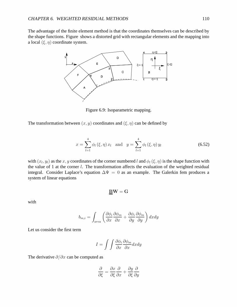
The advantage of the finite element method is that the coordinates themselves can be described bythe shape functions. Figure shows a distorted grid with rectangular elements and the mapping intoa local (ξ, η) coordinate system.
η
ξξ=−1 ξ=+1
η=−1
η=+1
� �
��
�
�
�
�
�
�
�
�
�
�
�
Figure 6.9: Isoparametric mapping.
The transformation between (x, y) coordinates and (ξ, η) can be defined by
x =
4∑
l=1
φl (ξ, η)xl and y =
4∑
l=1
φl (ξ, η) yl (6.52)
with (xl, yl) as the x, y coordinates of the corner numbered l and φl (ξ, η) is the shape function withthe value of 1 at the corner l. The transformation affects the evaluation of the weighted residualintegral. Consider Laplace’s equation ∆Ψ = 0 as an example. The Galerkin fem produces asystem of linear equations
BW = G
with
bm,i =
∫
area
(∂φi
∂x
∂φm
∂x+
∂φi
∂y
∂φm
∂y
)dxdy
Let us consider the first term
I =
∫ ∫∂φi
∂x
∂φm
∂xdxdy
The derivative ∂/∂x can be computed as
∂
∂ξ=
∂x
∂ξ
∂
∂x+
∂y
∂ξ
∂
∂y
CHAPTER 6. WEIGHTED RESIDUAL METHODS 111
such that ∂φ/∂x and ∂φ/∂y are related to ∂φ/∂ξ and ∂φ/∂η by
(∂φ/∂ξ∂φ/∂η
)= [J]
(∂φ/∂x∂φ/∂y
)(6.53)
with [J] =
(∂x/∂ξ ∂y/∂ξ∂x/∂η ∂y/∂η
)(6.54)
where [J] is the Jacobian. The derivatives in the Jacobian can easily be computed from the map-ping (6.52), e.g.,
∂y
∂ξ=
4∑
l=1
(∂φl
∂ξ(ξ, η)
)yl
From (6.53) one can determine the following explicit formulation for ∂φ/∂x
∂φi
∂x=
1
det J
(∂y
∂ξ
∂φi
∂η−
∂y
∂η
∂φi
∂ξ
)(6.55)
Exercise: Derive equation (6.55).
Using dxdy = detJ dξdη one obtains
I =
∫ 1
−1
∫ 1
−1
1
detJ
[(∂y
∂ξ
∂φi
∂η−
∂y
∂η
∂φi
∂ξ
)(∂y
∂ξ
∂φm
∂η−
∂y
∂η
∂φm
∂ξ
)]dξdη
All derivatives in this formulation are known because of the simple form that the φl assume. Theintegral can evaluated numerically or analytically.
6.4 Spectral method
The Galerkin spectral method is similar to the traditional Galerkin method but uses a suitable setof orthogonal functions such that
∫φkφldx
{6= 0 for k 6= l= 0 for k = l
Example for such functions are Fourier series, Legendre, or Chebyshev polynomials. In this sensethe spectral methods can be considered global methods rather than local as in the case of finitedifferences or finite elements.
CHAPTER 6. WEIGHTED RESIDUAL METHODS 112
6.4.1 Diffusion equation
Consider as an example the diffusion equation
∂T
∂t= α
∂2T
∂x2
for x ∈ [0, 1] and the boundary and initial conditions
T (0, t) = 0, T (1, t) = 1, and T (x, 0) = sin (πx) + x
Approximate solution
T = sin (πx) + x +N∑
j=1
aj(t) sin (jπx)
where the aj(t) are the unknown coefficients which need to be determined. This yields the residual
R =
N∑
j=1
[daj
dt+ α (jπ)2 aj
]sin (jπx) + απ2 sin (πx)
Evaluation of the weighted integral∫
R sin (mπx) dx yields
N∑
j=1
[daj
dt+ α (jπ)2 aj
]∫ 1
0
sin (jπx) sin (mπx) dx + απ2
∫ 1
0
sin (πx) sin (mπx) dx = 0
The integral yield
∫ 1
0
sin (jπx) sin (mπx) dx =
{1/2 for j = m0 for j 6= m
∫ 1
0
sin (πx) sin (mπx) dx =
{1/2 for m = 10 for m 6= 1
which yields
dam
dt+ α (jπ)2 am + rm = 0, m = 1, ..., N
rm =
{απ2 for m = 10 for m 6= 1
CHAPTER 6. WEIGHTED RESIDUAL METHODS 113
with the solution
a1 = e−απ2t − 1
am = 0
The solution for T is therefore
T = sin (πx) e−απ2t + x
This is in fact the exact solution, however, this has been obtained for this particular set of initialand boundary conditions. For a more realistic case of
T (x, 0) = 5x − 4x2
and replacing sin (πx) + x with 5x − 4x2 in the trial solution one obtains
rm =
{16αm
for m = 1, 3, 5, ...0 for m = 2, 4, 6, ...
With forward time differencing dam/dt = (an+1m − an
m) /∆t one obtains
an+1m = an
m − ∆t[α (jπ)2 an
m + rm
]
Table 6.8: Value of the solution at x = 0.5 for different timest N=1 N=3 n=5 Exact solution
0 1.5 1.5 1.5 1.50.1 0.851 0.889 0.881 0.8850.2 0.610 0.648 0.640 0.643
Table 6.8 shows the value of T for selected times and different values of N at x = 0.5. Note thatthe error is caused by two sources one of which is the limited accuracy of the representation interms of the base functions and the other is the error in the temporal integration.
Notes:
• The spectral method achieves relatively high accuracy with relatively few unknowns.
• For Dirichlet conditions the method reduces the problem to a set of ordinary differentialequations
• Treatment of nonlinear terms is not yet clear (and can be difficult)
CHAPTER 6. WEIGHTED RESIDUAL METHODS 114
6.4.2 Neumann boundary conditions
Let us now consider the diffusion equation again, however, for Neumann boundary conditions.Specifically the initial and boundary conditions are
T (x, 0) = 3 − 2x − 2x2 + 2x3,
∂T
∂x(0, t) = −2.0 and T (1, t) = 1.0
Different from the prior example it is not attempted to incorporate the initial and boundary condi-tions into the approximate solution. Rather a general trial solution is used
T (x, t) = b0(t) +N∑
j=1
[aj(t) sin (j2πx) + bj(t) cos (j2πx)]
The boundary conditions require the following relations for the coefficients
N∑
j=1
aj2πj = −2 ,
N∑
j=0
bj = 1
which can be used to eliminate aN and bN from the the approximate solution:
aN = −1
πN−
N−1∑
j=1
ajj
N, bN = 1 −
N−1∑
j=0
bj
This yields for the approximate solution
T (x, t) = cos (N2πx) −1
πNsin (N2πx) +
N−1∑
j=1
aj(t)
[sin (j2πx) −
j
Nsin (N2πx)
]
+N−1∑
j=0
bj(t) [cos (j2πx) + cos (N2πx)]
This implies that the terms in square brackets now need to be considered as the base functions or
wma= sin (m2πx) −
m
Nsin (N2πx) , 1 ≤ m ≤ N − 1
wmb= cos (m2πx) + cos (N2πx) , 0 ≤ m ≤ N − 1
CHAPTER 6. WEIGHTED RESIDUAL METHODS 115
Substitution into the the diffusion equation yields the residual
R =
N−1∑
j=1
{[daj
dt+ α (2πj)2 aj
]sin (2πjx) −
[daj
dt+ α (2πN)2 aj
]j
Nsin (2πNx)
}
+
N−1∑
j=0
{[dbj
dt+ α (2πj)2 bj
]cos (2πjx) +
[dbj
dt+ α (2πN)2 bj
]cos (2πNx)
}
+α (2πN)2 cos (2πNx) − α4πN sin (2πNx)
Evaluating the weighted residuals yields
dam
dt+ α (2πm)2 am +
m
N
N−1∑
j=1
j
N
[daj
dt+ α (2πN)2 aj
]= −α4πN (6.56)
dbm
dt+ α (2πm)2 bm +
N−1∑
j=0
[dbj
dt+ α (2πN)2 bj
]= α (2πN)2 (6.57)
2db0
dt+
N−1∑
j=0
[dbj
dt+ α (2πN)2 bj
]= α (2πN)2 (6.58)
Equations (6.56) for am are linearly independent from equations (6.57) and can be solved indepen-dently. To solve for the time integration it is necessary, however, to factorize the the system andcarry out a matrix multiplication for each time step. Start values for am and bm are easily obtainedusing the trial solution for the initial condition.
Note, since the problem is linear the factorization is only needed once because the subsequent timesteps always use the same matrix (coefficients in equations (6.56) to (6.58) are constant).
6.4.3 Pseudospectral method
Main disadvantage of spectral method is large computational effort particularly for nonlinear prob-lems. An alternative to Galerkin method which basically solve the diffusion equation in spectralspace is to use a mixture of spectral and real space. An frequently used method in this category isthe pseudospectral approach which uses the collocation method. The example is again the diffusionequation
∂u
∂t− α
∂2u
∂x2= 0
subject to the boundary and initial conditions
u (−1, t) = −1, u (1, t) = 1, u (x, 0) = sin πx + x
CHAPTER 6. WEIGHTED RESIDUAL METHODS 116
When compared to the spectral method, the pseudospectral method does not determine the solutionentirely in spectral space. Recall that the solution for the Galerkin spectral method is found byintegrating the spectral coefficients. For a linear problem this is feasible but a nonlinear problemrequires the inversion of a large matrix for each time step.
The pseudo spectral method often uses an expansion
u (x, t) =N+1∑
k=1
ak (t) Tk−1 (x)
consists of three basic steps:
• Given a solution unj one determines the spectral coefficients ak. This transforms the problem
from physical to spectral space. Using Chebichev Polynomials the step can be done with a
fast Fourier Transform (FFT) if the collocation points are xj = cos(
π(j−1)N
)(time efficient
with number of operations proportional to N log N ).
• The next step is to evaluate the second derivative ∂2u/∂x2 from the coefficients ak whichmakes use of recurrence relations and is also very efficient:
∂u
∂x=
N+1∑
k=1
a(1)k Tk−1 (x)
∂2u
∂x2=
N+1∑
k=1
a(2)k Tk−1 (x)
• The final step then is to integrate in time. Different from the Galerkin spectral method this is
done in real space directly for u: un+1j = un
j + α∆t ∂2u∂x2
∣∣∣n
jthereby avoiding to have to solve
a large system of equations for the time derivatives of dak/dt.
6.5 Summary on different weighted residual methods:
• local approximations: finite difference, finite volume, finite element
– irregular domains
– variable grid resolution
– boundary conditions relatively simple
• global base function: spectral methods
– high accuracy

CHAPTER 6. WEIGHTED RESIDUAL METHODS 117
– arbitrary often differentiable
– Galerkin method computationally expensive for nonlinear problems
– Pseudospectral method employs spectral space only to determine spatial derivatives(much more efficient)