Joel PrimackUniversity of California, Santa Cruz

Week 9Cosmic Web

Physics 224 - Spring 2010

Origin and Evolution of the Universe

Physics 224 - Spring 2010

Origin and Evolution of the UniverseWeek Topics

1 Historical Introduction2 General Relativistic Cosmology3 Big Bang Nucleosynthesis4 Recombination, Dark Matter5 Dark Matter, Topological Defects6 Cosmic Inflation7 Before and After Cosmic Inflation8 Baryogenesis, CMB, Structure Formation9 Cosmic Web10 Galaxy Formation and Evolution11 Student Presentations

≈

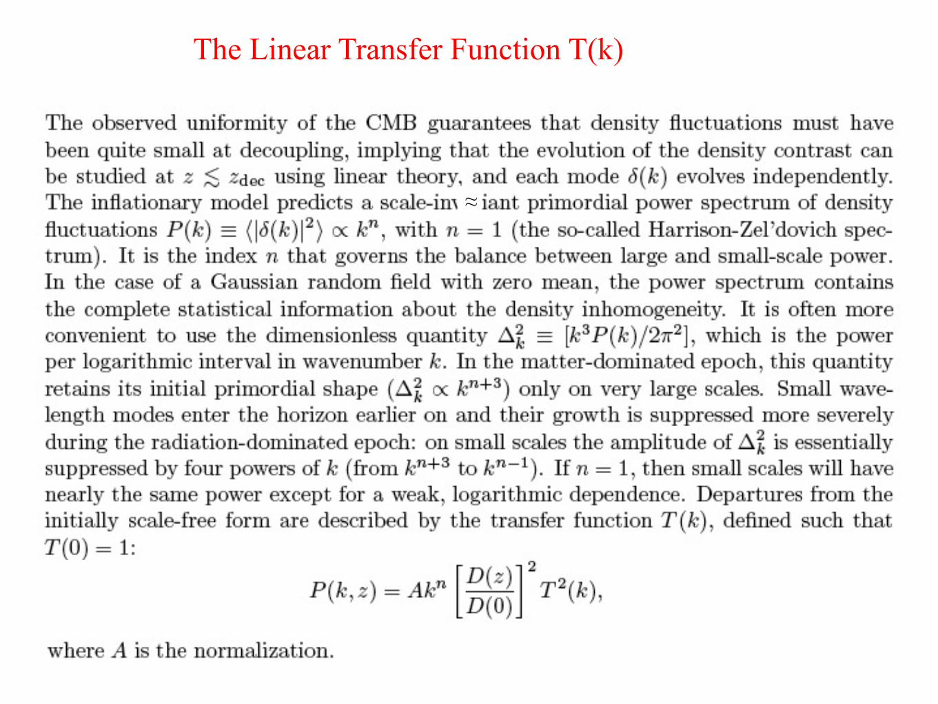
The Linear Transfer Function T(k)

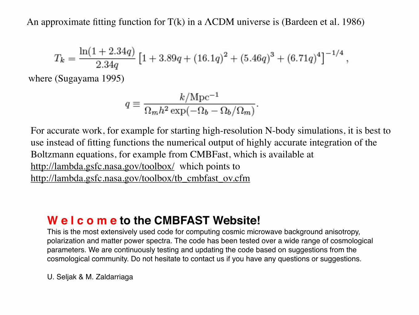
An approximate fitting function for T(k) in a ΛCDM universe is (Bardeen et al. 1986)

where (Sugayama 1995)

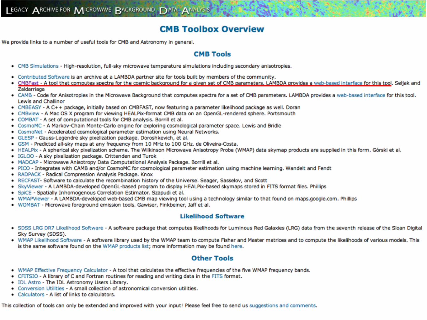
For accurate work, for example for starting high-resolution N-body simulations, it is best to use instead of fitting functions the numerical output of highly accurate integration of the Boltzmann equations, for example from CMBFast, which is available at http://lambda.gsfc.nasa.gov/toolbox/ which points to http://lambda.gsfc.nasa.gov/toolbox/tb_cmbfast_ov.cfm

W e l c o m e to the CMBFAST Website!This is the most extensively used code for computing cosmic microwave background anisotropy, polarization and matter power spectra. The code has been tested over a wide range of cosmological parameters. We are continuously testing and updating the code based on suggestions from the cosmological community. Do not hesitate to contact us if you have any questions or suggestions.

U. Seljak & M. Zaldarriaga

Scale-Invariant Spectrum (Harrison-Zel’dovich)

mass

t time

M

δ

M

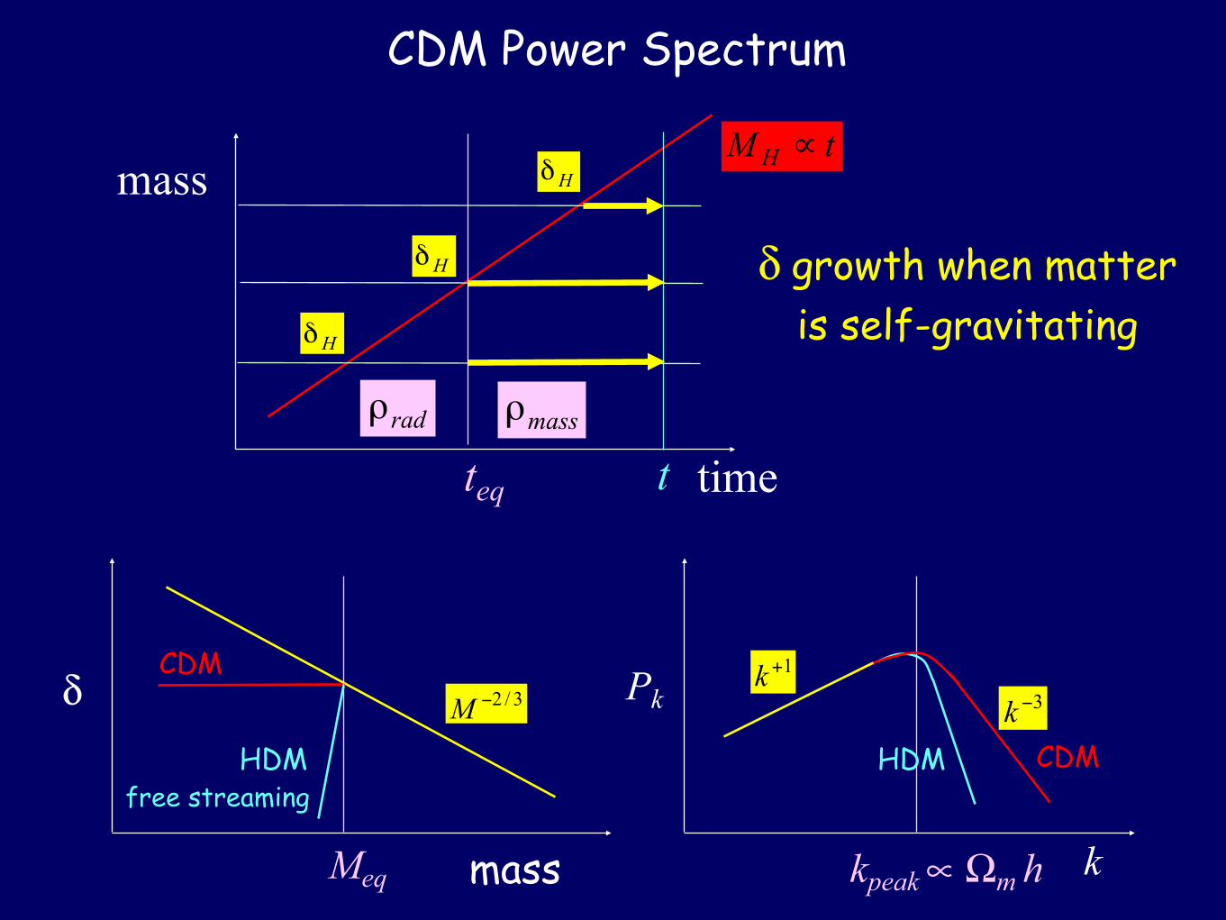
CDM Power Spectrum

δ

Meq mass

CDM

HDM free streaming

mass

t timeteq

δ growth when matter is self-gravitating

Pk

kpeak ∝ Ωm h k

CDMHDM

Formation of Large-Scale Structure

M

1

0

CDM: bottom-up

Fluctuation growth in the linear regime:

HDM: top-down

M

1

0

free streaming

rms fluctuation at mass scale M:

Galaxies Clusters Superclusters Galaxies Clusters Superclusters

From Peter Schneider, Extragalactic Astronomy and Cosmology (Springer, 2006)

Einstein-de Sitter

Open universe

Benchmark model

Structure formsearliest in Open,next in Benchmark,latest in EdS model.

Open

Benchmark

EdS

Linear Growth Rate Function D(a)

From Klypin, Trujillo, Primack - Bolshoi paper 1 - Appendix A

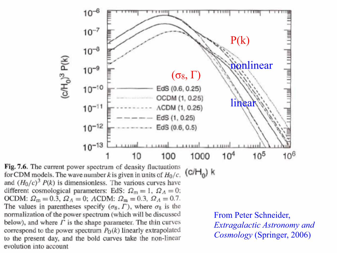
From Peter Schneider, Extragalactic Astronomy and Cosmology (Springer, 2006)

(σ8, Γ)

P(k)

nonlinear

linear

On large scales (k small), the gravity of the dark matter dominates. But on small scales, pressure dominates and growth of baryonic fluctuations is prevented. Gravity and pressure are equal at the Jeans scale

The Jeans mass is the dark matter + baryon mass enclosed within a sphere of radius πa/kJ,

where µ is the mean molecular weight. The evolution of MJ is shown below, assuming that reionization occurs at z=15:

Jeans-type analysis for HDM, WDM, and CDM

Hot Dark Matter

Warm Dark Matter

Cold Dark Matter

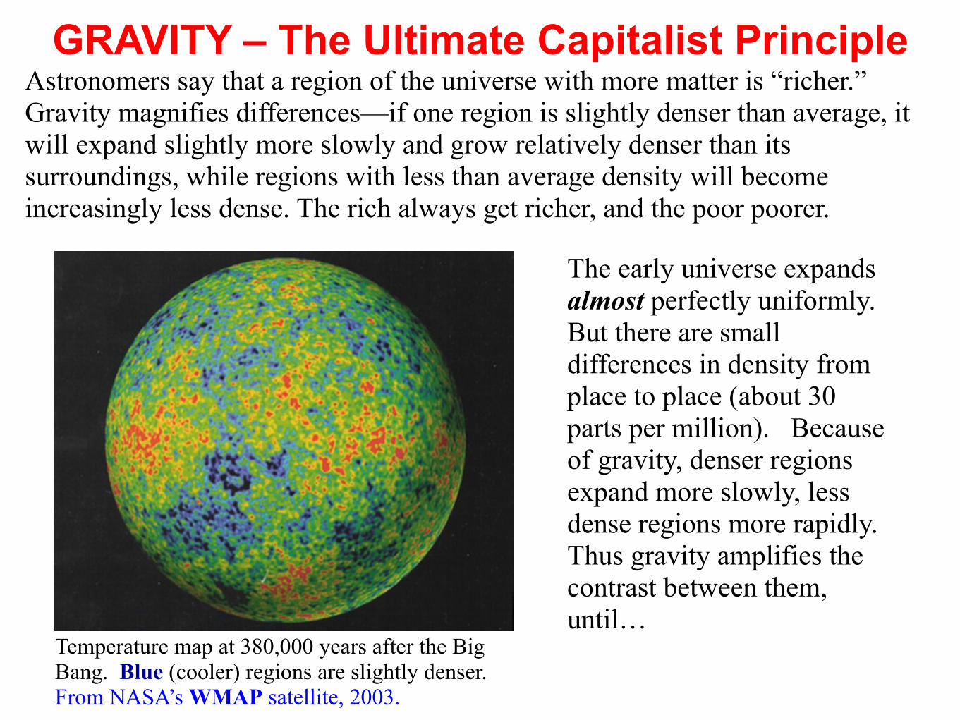
GRAVITY – The Ultimate Capitalist Principle

The early universe expands almost perfectly uniformly. But there are small differences in density from place to place (about 30 parts per million). Because of gravity, denser regions expand more slowly, less dense regions more rapidly. Thus gravity amplifies the contrast between them, until…

Astronomers say that a region of the universe with more matter is “richer.” Gravity magnifies differences—if one region is slightly denser than average, it will expand slightly more slowly and grow relatively denser than its surroundings, while regions with less than average density will become increasingly less dense. The rich always get richer, and the poor poorer.

Temperature map at 380,000 years after the Big Bang. Blue (cooler) regions are slightly denser. From NASA’s WMAP satellite, 2003.

Structure Formation by Gravitational Collapse

When any region becomes about twice as dense as typical regions its size, it reaches a maximum radius, stops expanding,

and starts falling together. The forces between the subregions generate velocities which prevent the material from all falling toward the center.

Through Violent Relaxation the dark matter quickly reaches a stable configuration that’s about half the maximum radius but denser in the center.Simulation of top-hat collapse: P.J.E. Peebles 1970, ApJ, 75, 13.

TOP HAT VIOLENT VIRIALIZEDMax Expansion RELAXATION

rmax rvir

Growth and Collapse of Fluctuations

Schematic sketches of radius, density, and density contrast of an overdense fluctuation. It initially expands with the Hubble expansion, reaches a maximum radius (solid vertical line), and undergoes violent relaxation during collapse (dashed vertical line), which results in the dissipationless matter forming a stable halo. Meanwhile the ordinary matter ρb continues to dissipate kinetic energy and contract, thereby becoming more tightly bound, until dissipation is halted by star or disk formation, explaining the origin of galactic spheroids and disks. (This was the simplified discussion of BFPR84; the figure is from my 1984 lectures at the Varenna school.Now we take into account halo growth by accretion, and the usual assumption is that spheroids form mostly as a result of galaxy mergers Toomre 1977.)

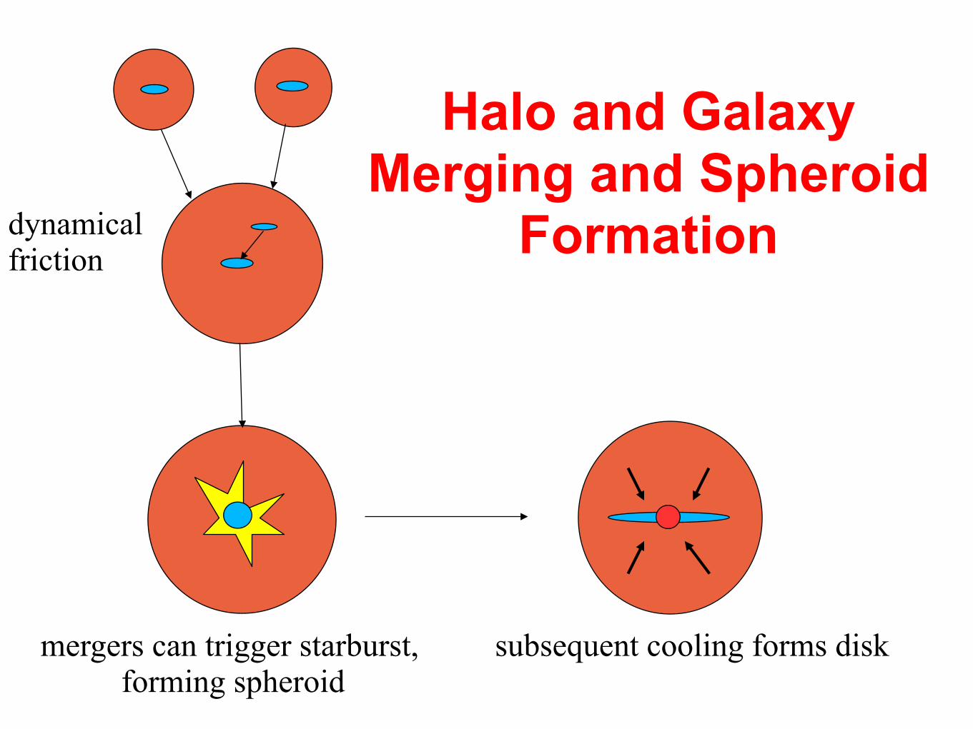
Halo and Galaxy Merging and Spheroid

Formationdynamicalfriction

mergers can trigger starburst, forming spheroid

subsequent cooling forms disk

Growth Factor

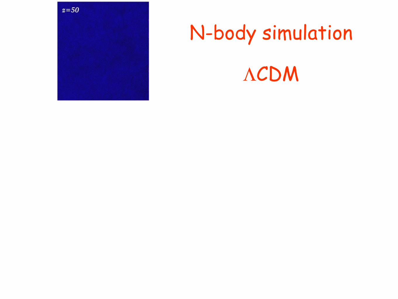
N-body simulationN-body simulation

ΛCDM

N-body simulation

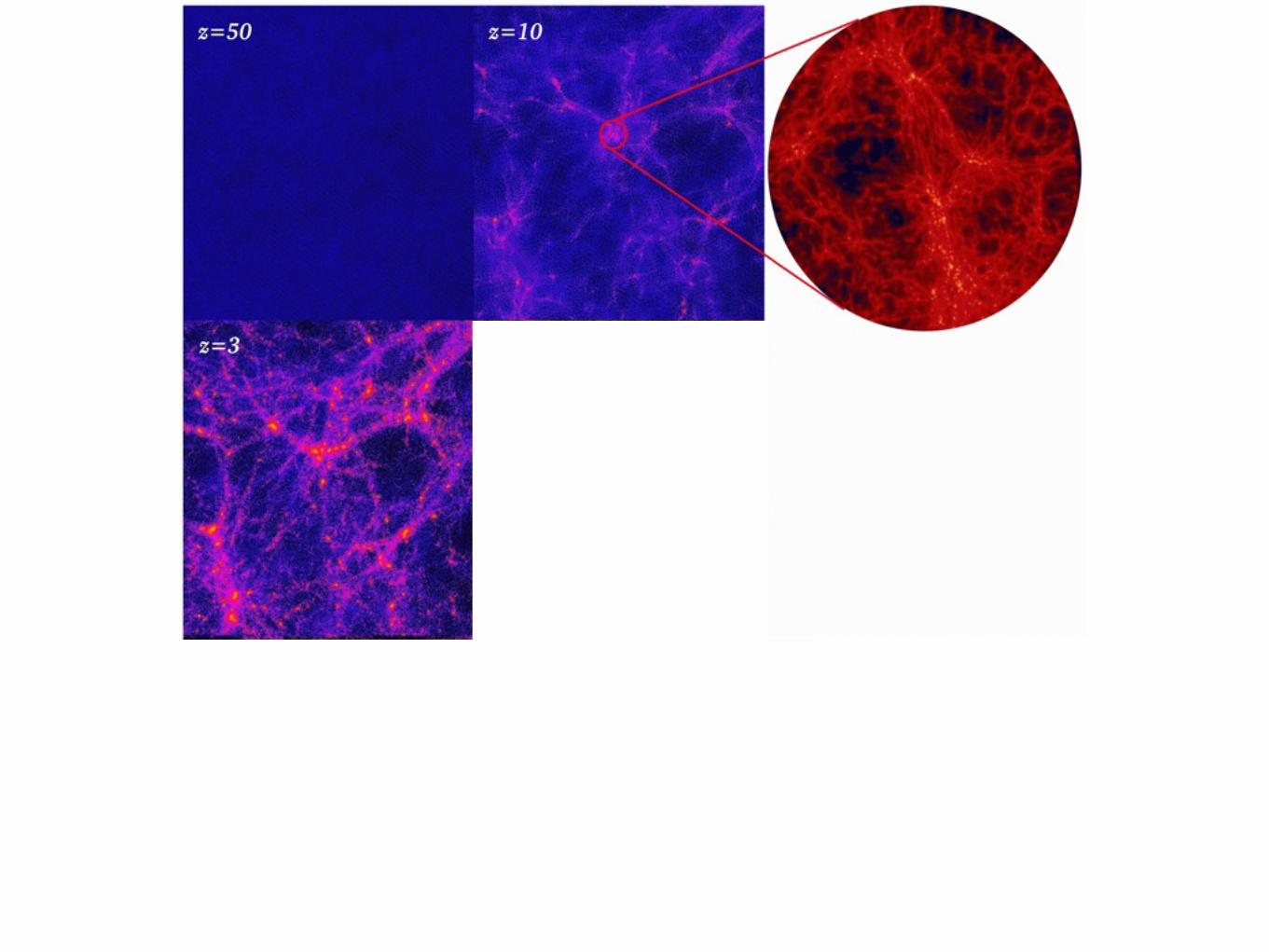
N-body simulation

Micro-Macro Connection

Cold Dark Matter

Hot Dark Matterν

24

ColumbiaSuper

computerNASA Ames

Simulation:Brandon Allgood & Joel Primack

Visualization:ChrisHenze

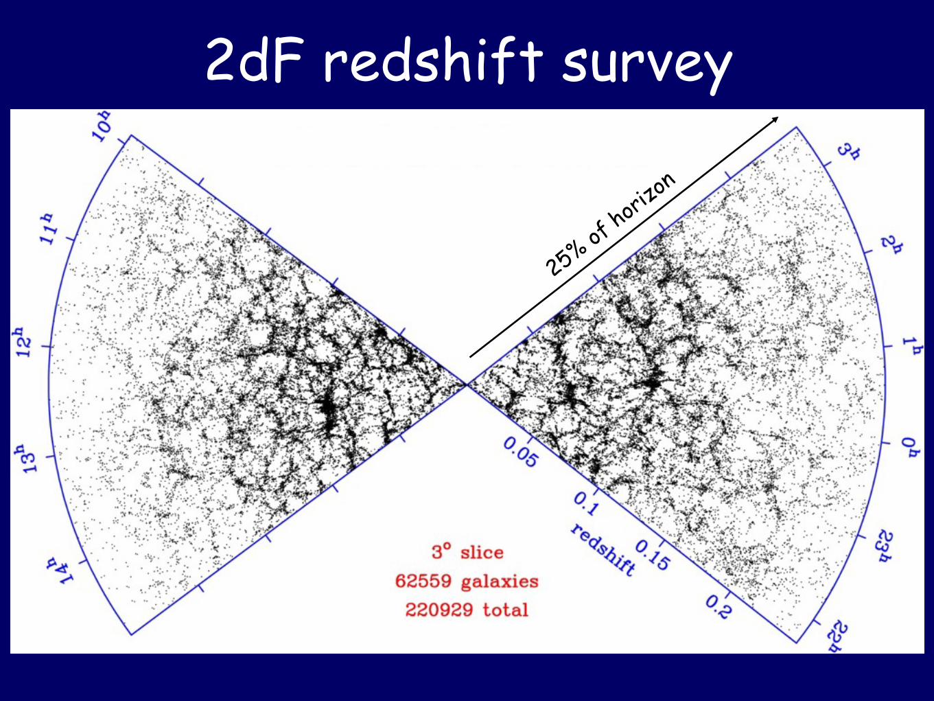
2dF redshift survey

25% of hori

zon

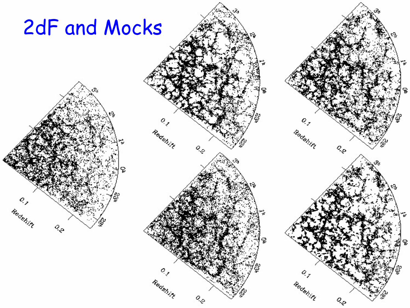
2dF and Mocks

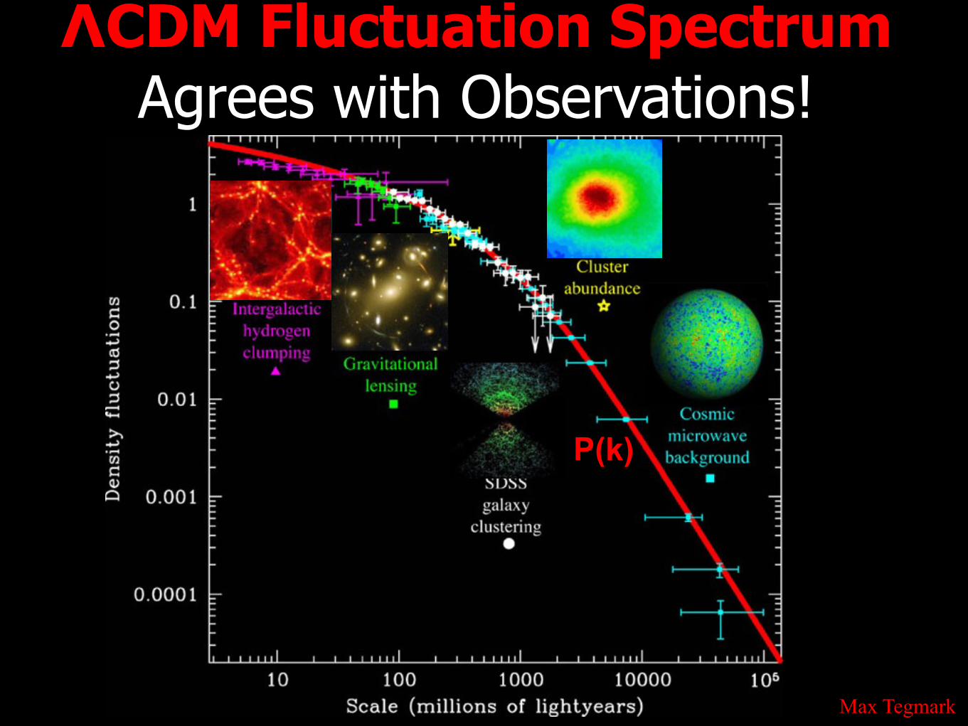
ΛCDM Fluctuation Spectrum Agrees with Observations!

Max Tegmark

P(k)

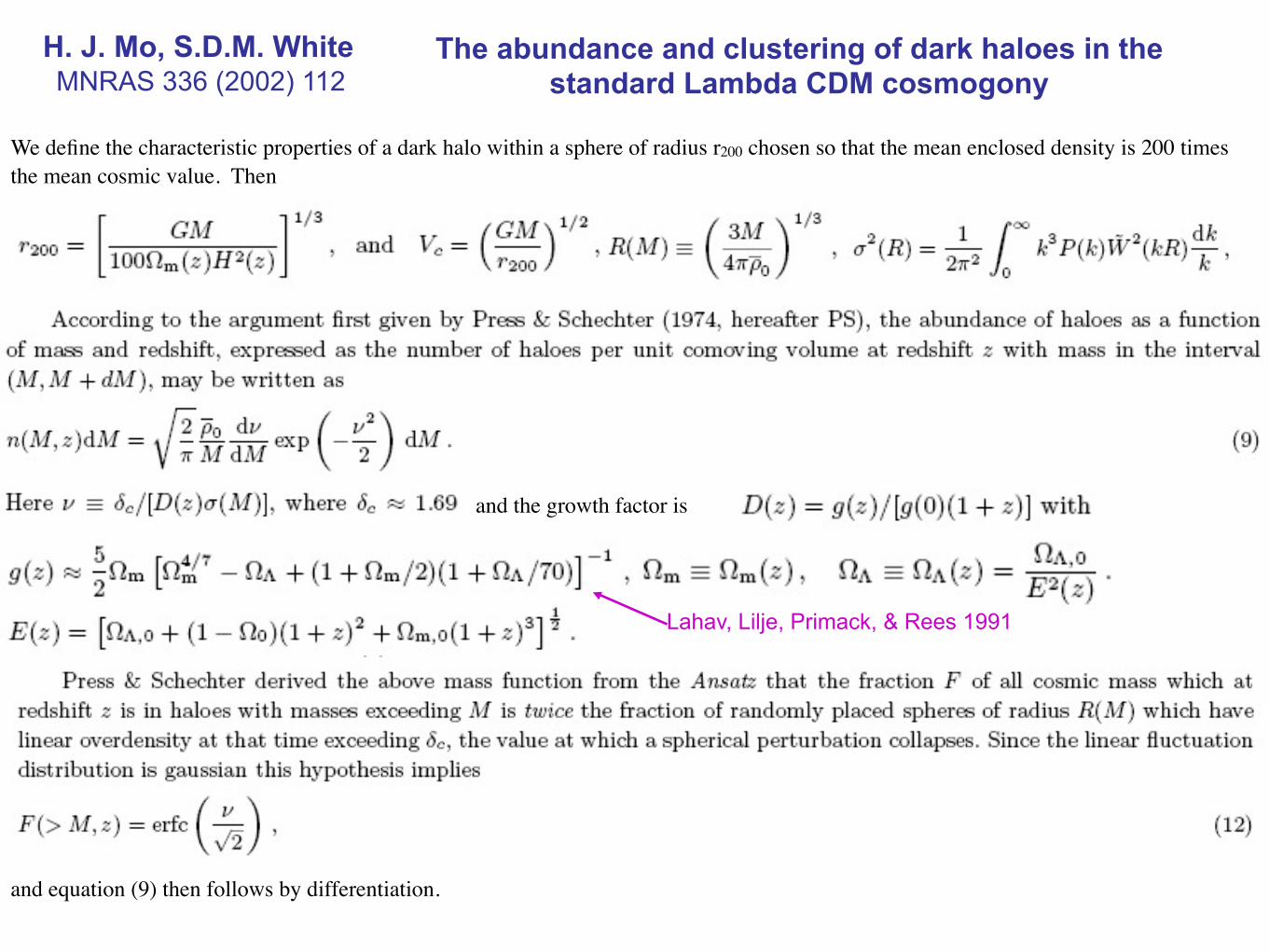
MNRAS 336 (2002) 112 The abundance and clustering of dark haloes in the

standard Lambda CDM cosmogony H. J. Mo, S.D.M. White

We define the characteristic properties of a dark halo within a sphere of radius r200 chosen so that the mean enclosed density is 200 times the mean cosmic value. Then

and the growth factor is

and equation (9) then follows by differentiation.

Lahav, Lilje, Primack, & Rees 1991

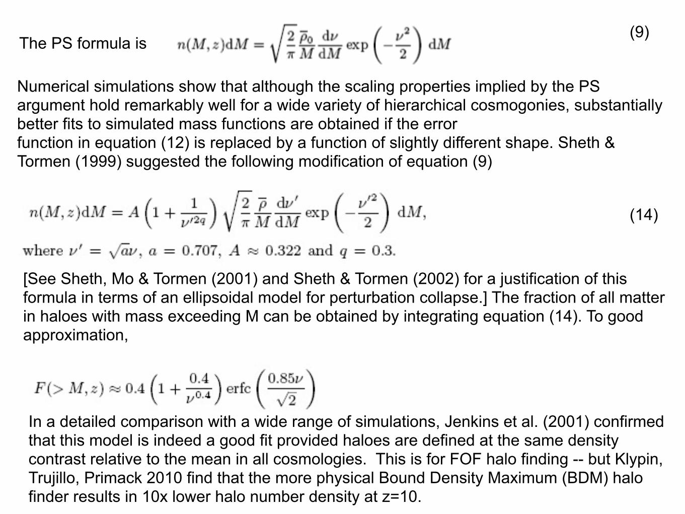
Numerical simulations show that although the scaling properties implied by the PS argument hold remarkably well for a wide variety of hierarchical cosmogonies, substantially better fits to simulated mass functions are obtained if the errorfunction in equation (12) is replaced by a function of slightly different shape. Sheth & Tormen (1999) suggested the following modification of equation (9)

[See Sheth, Mo & Tormen (2001) and Sheth & Tormen (2002) for a justification of this formula in terms of an ellipsoidal model for perturbation collapse.] The fraction of all matter in haloes with mass exceeding M can be obtained by integrating equation (14). To good approximation,

In a detailed comparison with a wide range of simulations, Jenkins et al. (2001) confirmed that this model is indeed a good fit provided haloes are defined at the same density contrast relative to the mean in all cosmologies. This is for FOF halo finding -- but Klypin, Trujillo, Primack 2010 find that the more physical Bound Density Maximum (BDM) halo finder results in 10x lower halo number density at z=10.

The PS formula is

(14)

(9)

z = 8.8

Curve: Sheth- Tormen approx.

FOF halos link = 0.20SO halos

Sheth-Tormen approximation with the same WMAP5 parameters used for Bolshoi simulation very accurately agrees with abundance of halos at low redshifts, but increasingly overpredicts bound spherical overdensity halo abundance at higher redshifts.

Sheth-Tormen Fails atHigh Redshifts

Klypin, Trujillo, & Primack, arXiv: 1002.3660v3

Each panel shows 1/2 of the dark matter particles in cubes of 1h-1 Mpc size. The center of each cube is the exact position of the center of mass of the corresponding FOF halo. The effective radius of each FOF halo in the plots is 150 − 200 h-1 kpc. Circles indicate virial radii of distinct halos and subhalos identified by the spherical overdensity algorithm BDM.

= ratio of FOF mass / SO mass

FOF linked together a chain of halos that formed in long and dense filaments (also in panels b, d, f, h; e = major merger)

Klypin, Trujillo, & Primack, arXiv: 1002.3660v3

FOF

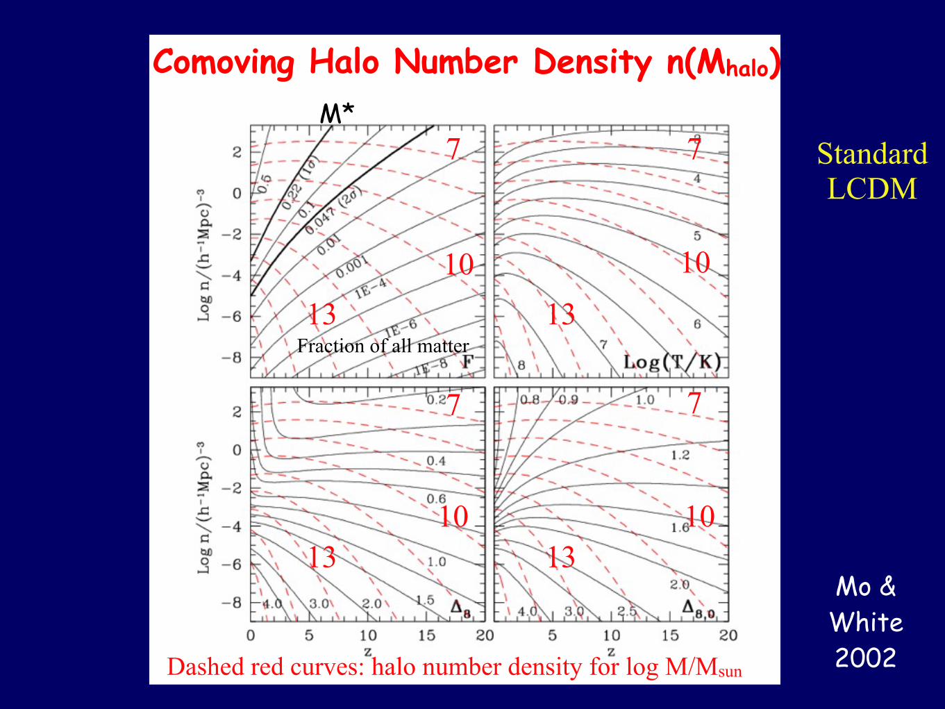
Comoving Halo Number Density n(Mhalo)

Mo & White 2002

Mo & White 2002

Standard LCDM

Fraction of all matter

Dashed red curves: halo number density for log M/Msun

7

1013

M*7

77

10

1010

13

1313

Comoving Halo Number Density n(Mhalo)

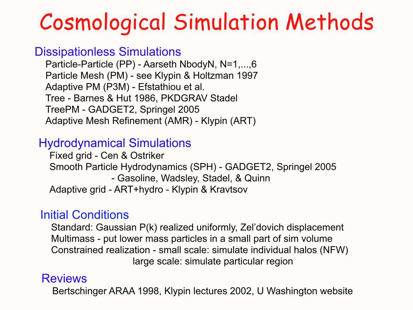
Cosmological Simulation MethodsDissipationless Simulations

Particle-Particle (PP) - Aarseth NbodyN, N=1,...,6Particle Mesh (PM) - see Klypin & Holtzman 1997Adaptive PM (P3M) - Efstathiou et al.Tree - Barnes & Hut 1986, PKDGRAV StadelTreePM - GADGET2, Springel 2005Adaptive Mesh Refinement (AMR) - Klypin (ART)

Hydrodynamical SimulationsFixed grid - Cen & OstrikerSmooth Particle Hydrodynamics (SPH) - GADGET2, Springel 2005 - Gasoline, Wadsley, Stadel, & QuinnAdaptive grid - ART+hydro - Klypin & Kravtsov

Initial ConditionsStandard: Gaussian P(k) realized uniformly, Zel’dovich displacementMultimass - put lower mass particles in a small part of sim volumeConstrained realization - small scale: simulate individual halos (NFW)

large scale: simulate particular region

ReviewsBertschinger ARAA 1998, Klypin lectures 2002, U Washington website

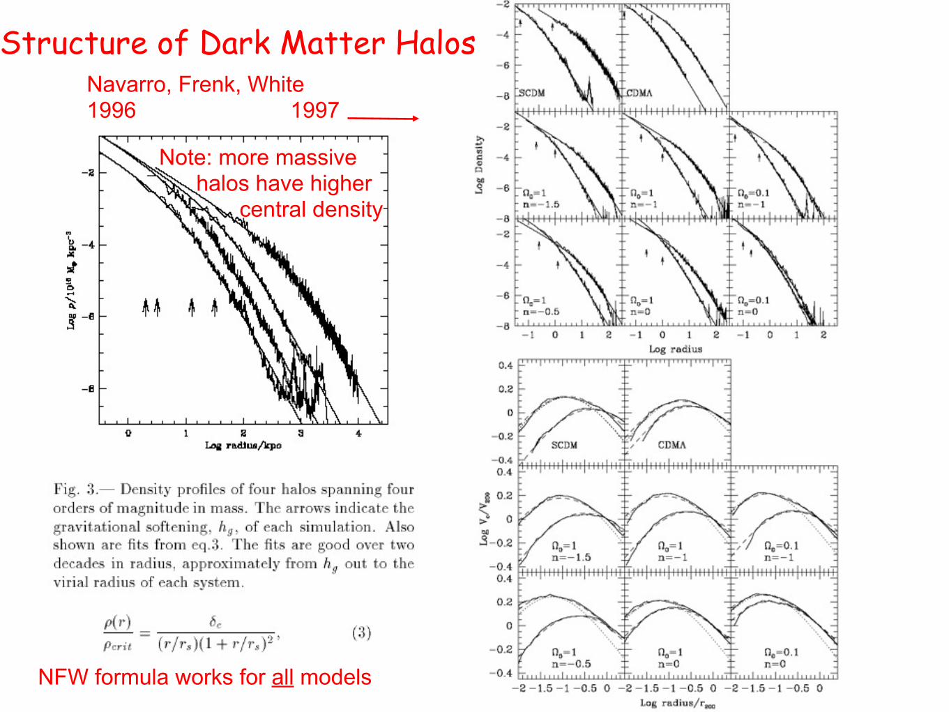
Navarro, Frenk, White1996 1997

Structure of Dark Matter Halos

NFW formula works for all models

Note: more massive halos have higher central density

Table 2

Comparison of NFW and Moore et al. profiles

Parameter NFW Moore et al.

Density ! = !s

x(1 + x)2! = !s

x1.5(1 + x)1.5

x = r/rs ! ! x!3 for x " 1 ! ! x!3 for x " 1! ! x!1 for x # 1 ! ! x!1.5 for x # 1!/!s = 1/4 at x = 1 !/!s = 1/2 at x = 1

MassM = 4"!sr3

sf(x) f(x) = ln(1 + x) $ x1 + x f(x) = 2

3 ln(1 + x3/2)

= Mvirf(x)/f(C)Mvir = 4!

3 !cr!0#top!hatr3vir

Concentration CNFW = 1.72CMoore CMoore = CNFW/1.72for halos with the same Mvir and rmax

C = rvir/rs C1/5 % CNFW0.86f(CNFW) + 0.1363

C1/5 = CMoore

[(1 + C3/2Moore)

1/5 $ 1]2/3

error less than 3% for CNFW =5-30 % CMoore

[C3/10Moore $ 1]2/3

C"=!2 = CNFW C"=!2 = 23/2CMoore

% 2.83CMoore

Circular Velocity

v2circ =

GMvir

rvir

C

x

f(x)

f(C)xmax % 2.15 xmax % 1.25

= v2max

xmax

x

f(x)

f(xmax)v2max % 0.216v2

vir

C

f(C)v2max % 0.466v2

vir

C

f(C)

v2vir =

GMvir

rvir!/!s % 1/21.3 at x = 2.15 !/!s % 1/3.35 at x = 1.25

9

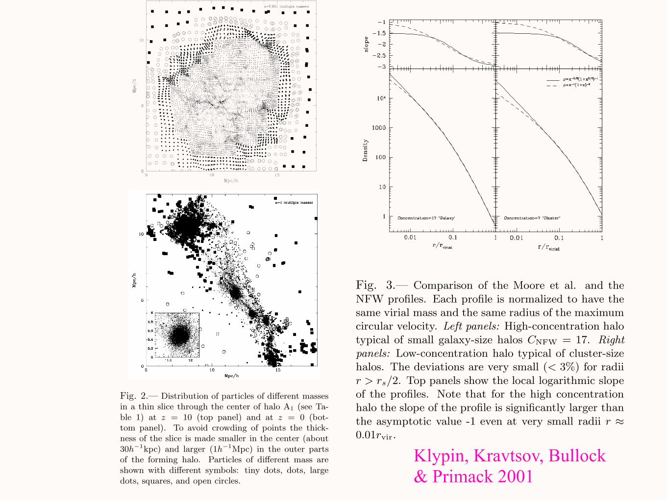
Dark Matter Halo Radial Profile

Klypin, Kravtsov, Bullock & Primack 2001

the radius at which the logarithmic slope of thedensity profile is equal to !2. This scale corre-sponds to rs for the NFW profile and " 0.35rs forthe Moore et al. profile.

Figure 3 presents the comparison between theanalytic profiles normalized to have the same virialmass and the same radius rmax. We show resultsfor halos of low and high values of concentrationrepresentative of cluster- and low-mass galaxy ha-los, respectively. The bottom panels show the pro-files, while the top panels show the correspondinglogarithmic slope as a function of radius. The fig-ure shows that the two profiles are very similarthroughout the main body of the halos. Only inthe very central region do the di!erences becomesignificant. The di!erence is more apparent in thelogarithmic slope than in the actual density pro-files. Moreover, for galaxy-mass halos the di!er-ence sets in at a rather small radius ! 0.01rvir,which would correspond to scales < 1 kpc for thetypical dark matter dominated dwarf and LSBgalaxies. At the observationally interesting scalesthe di!erences between NFW and Moore et al.profiles are fairly small and the NFW profile pro-vides an accurate description of the halo densitydistribution.

Note also that for galaxy-size (e.g., high-concentration) halos the logarithmic slope of theNFW profile has not yet reached its asymptoticinner value of !1 even at scales as small as0.01rvir. At this distance the logarithmic slopeof the NFW profile is " !1.4 ! 1.5 for halos withmass # 1012h!1M". For cluster-size halos thisslope is " !1.2. This dependence of the slope at agiven fraction of the virial radius on the virial massof the halo is very similar to the results plottedin Figure 3 of Jing & Suto (2000). These authorsinterpreted it as evidence that halo profiles arenot universal. It is obvious, however, that theirresults are consistent with NFW profiles and thedependence of the slope on mass can be simply amanifestation of the well-studied cvir(M) relation.

The NFW and Moore et al. profiles can becompared in a di!erent way. We can approximatethe Moore et al. halo of a given concentration withthe NFW profile. Fractional deviations of the fitsdepend on the halo concentration and on the rangeof radii used for the fits. A low-concentration halohas larger deviations, but even for C = 7 case, thedeviations are less than 15% if we fit the halo at

Fig. 3.— Comparison of the Moore et al. and theNFW profiles. Each profile is normalized to have thesame virial mass and the same radius of the maximumcircular velocity. Left panels: High-concentration halotypical of small galaxy-size halos CNFW = 17. Right

panels: Low-concentration halo typical of cluster-sizehalos. The deviations are very small (< 3%) for radiir > rs/2. Top panels show the local logarithmic slopeof the profiles. Note that for the high concentrationhalo the slope of the profile is significantly larger thanthe asymptotic value -1 even at very small radii r !

0.01rvir.

scales 0.01 < r/rvir < 1. For a high-concentrationhalo with C = 17, the deviations are much smaller:less than 8% for the same range of scales.

To summarize, we find that the di!erences be-tween the NFW and the Moore et al. profiles arevery small ("!/! < 10%) for radii above 1% ofthe virial radius for typical galaxy-size halos withCNFW

># 12. The di!erences are larger for haloswith smaller concentrations. In the case of theNFW profile, the asymptotic value of the centralslope " = !1 is not achieved even at radii as smallas 1%-2% of the virial radius.

3.2. Convergence study

The e!ects of numerical resolution can be stud-ied by resimulating the same objects with higherforce and mass resolution and with a larger num-ber of time steps. In this study we performed

8

Fig. 1.— Example of the construction of mass re-finement in lagrangian space (here for illustration weshow a 2D case). Three central blocks of particleswere marked for highest mass resolution. Each blockproduces 162 particles of the smallest mass. Adjacentblocks correspond to the four times lower resolutionand produce 82 particles each. The procedure is re-peated recursively until we reach the lowest level ofresolution. The region of the highest resolution canhave arbitrary shape.

Figure 2 shows an example of mass refinementfor one of the halos in our simulations. A largefraction of high resolution particles ends up inthe central halo, which does not have any largermass particles (see insert in the bottom panel). Atz = 10, the region occupied by the high resolutionparticles is non-spherical: it is substantially elon-gated in the direction perpendicular to the largefilament clearly seen at z = 0.

After the initial conditions are set, we run thesimulation again allowing the code to performmesh refinement based only on the number of par-ticles with the smallest mass.

2.3. Numerical simulations

We simulated a flat low-density cosmologicalmodel (!CDM) with "0 = 1 ! "! = 0.3, theHubble parameter (in units of 100 kms!1Mpc!1)h = 0.7, and the spectrum normalization !8 = 0.9.We have run two sets of simulations. The first set

Fig. 2.— Distribution of particles of di!erent massesin a thin slice through the center of halo A1 (see Ta-ble 1) at z = 10 (top panel) and at z = 0 (bot-tom panel). To avoid crowding of points the thick-ness of the slice is made smaller in the center (about30h!1kpc) and larger (1h!1Mpc) in the outer partsof the forming halo. Particles of di!erent mass areshown with di!erent symbols: tiny dots, dots, largedots, squares, and open circles.

used 1283 zeroth-level grid in a computational boxof 30h!1Mpc. The second set of simulations used2563 grid in a 25h!1Mpc box and had higher massresolution. In the simulations used in this paper,the threshold for cell refinement (see above) waslow on the zeroth level: nthresh(0) = 2. Thus, ev-

5

Klypin, Kravtsov, Bullock & Primack 2001

Aquarius Simulation: Formation of a Milky-Way-size Dark Matter Halo

Diameter of Milky Way Dark Matter Halo1.6 million light years

500 kpc

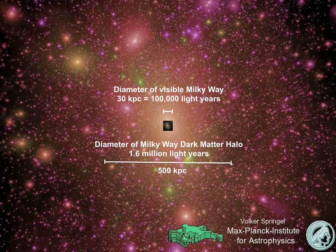
Diameter of visible Milky Way30 kpc = 100,000 light years

Diameter of Milky Way Dark Matter Halo1.6 million light years

500 kpc

Diameter of visible Milky Way30 kpc = 100,000 light years

Diameter of Milky Way Dark Matter Halo1.6 million light years