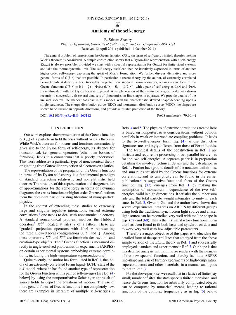
PHYSICAL REVIEW B 84, 165112 (2011)

Anatomy of the self-energy

B. Sriram ShastryPhysics Department, University of California, Santa Cruz, California 95064, USA

(Received 13 April 2011; published 11 October 2011)

The general problem of representing the Greens function G(k,z) in terms of self-energy in field theories lackingWick’s theorem is considered. A simple construction shows that a Dyson-like representation with a self-energy!(k,z) is always possible, provided we start with a spectral representation for G(k,z) for finite-sized systemsand take the thermodynamic limit. The self-energy itself can then be iteratively expressed in terms of anotherhigher order self-energy, capturing the spirit of Mori’s formulation. We further discuss alternative and moregeneral forms of G(k,z) that are possible. In particular, a recent theory, by the author, of extremely correlatedFermi liquids at density n, for Gutzwiller projected noncanonical Fermi operators, obtains a new form of theGreens function: G(k,z) = [(1 ! n

2 ) + "(k,z)]/[z ! Ek ! #(k,z)], with a pair of self-energies #(z) and "(z).Its relationship with the Dyson form is explored. A simple version of the two-self-energies model was shownrecently to successfully fit several data sets of photoemission line shapes in cuprates. We provide details of theunusual spectral line shapes that arise in this model, with the characteristic skewed shape depending upon asingle parameter. The energy distribution curve (EDC) and momentum distribution curve (MDC) line shapes areshown to be skewed in opposite directions, and provide a testable prediction of the theory.

DOI: 10.1103/PhysRevB.84.165112 PACS number(s): 79.60.!i

I. INTRODUCTION

Our work explores the representation of the Greens functionG(k,z) of a particle in field theories without Wick’s theorem.While Wick’s theorem for bosons and fermions automaticallygives rise to the Dyson form of self-energy, its absence fornoncanonical, i.e., general operators (other than bosons offermions), leads to a conundrum that is poorly understood.This work addresses a particular type of noncanonical theoryoriginating from Gutzwiller projection of electrons on a lattice.

The representation of the propagator or the Greens functionin terms of its Dyson self-energy is a fundamental paradigmof standard interacting relativistic and nonrelativistic fieldtheories. The structure of this representation and the generationof approximations for the self-energy in terms of Feynmandiagrams, the vertex function, or higher order Greens functionsform the dominant part of existing literature of many-particlephysics.

In the context of extending these studies to extremelylarge and singular repulsive interactions, termed extremecorrelations,1 one needs to deal with noncanonical electrons.A standard noncanonical problem involves the Hubbardoperators2 Xa,b

j located at sites j of a lattice. These are“graded” projection operators with label a representingthe three allowed local configurations 0, " , and #. Amongthese operators, X0$

j and X$0j are fermionic destruction- and

creation-type objects. Their Greens function is measured di-rectly in angle-resolved photoemission experiments (ARPES)on certain experimental systems embodying extreme correla-tions, including the high-temperature superconductors.3

Quite recently, the author has formulated in Ref. 1, the the-ory of an extremely correlated Fermi liquid (ECFL) state of thet-J model, where he has found another type of representationfor the Greens function with a pair of self-energies [see Eq. (4)below] by using the nonperturbative Schwinger approach ofsource fields to depict the equations of motion. The use ofmore general forms of Greens functions is not completely new,there are examples in literature of multiple self-energies in

Refs. 4 and 5. The physics of extreme correlations treated hereis based on nonperturbative considerations without obviousparallels in weak or intermediate coupling problems. It leadsto the two-self-energies form, Eq. (4), whose distinctivesignatures are strikingly different from those of Fermi liquids.

The technical details of the construction in Ref. 1 areintricate and require the processing of two parallel hierarchiesfor the two self-energies. A separate paper is in preparationdetailing the involved technical details and the calculation inRef. 1. Further background details of the notation, definitions,and sum rules satisfied by the Greens functions for extremecorrelations, and its analyticity can be found in the earlierpublication.2 A suggestive functional form of the Greensfunction, Eq. (37), emerges from Ref. 1, by making theassumption of momentum independence of the two self-energies, valid in high dimensions. It satisfies the number sumrule and the total particle weight integrates to unity in eachstate. In Ref. 3, Gweon, Gu, and the author have shown thatseveral experimental data sets on ARPES by different groupsusing both the traditional synchrotron light source and a laserlight source can be reconciled very well with the line shape inEqs. (37) and (60). This is the first satisfactory functional formthat has been found to fit both laser and synchrotron data andto work very well with few adjustable parameters.

Therefore a major objective of this paper is to elucidate thedetailed form of the spectral lines that emerged from the abovesimple version of the ECFL theory in Ref. 1 and successfullyemployed to understand experiments in Ref. 3. Our hope is thatthis detailed analysis will familiarize readers with the nuancesof the new spectral function, and thereby facilitate ARPESline-shape analysis of further experiments on high-temperaturesuperconductors and other materials, in a manner analogousto that in Ref. 3.

For the above purpose, we recall that in a lattice of finite (saysmall) number of sites, the state space is finite dimensional andhence the Greens function for arbitrarily complicated objectscan be computed by numerical means, leading to rationalfunctions of the complex frequency z as in Eq. (5) below.

165112-11098-0121/2011/84(16)/165112(13) ©2011 American Physical Society

B. SRIRAM SHASTRY PHYSICAL REVIEW B 84, 165112 (2011)

We begin by studying this representation and see how theDyson representation arises; we find that the two-self-energiesrepresentation, Eq. (4), is also quite natural from this viewpoint. We further study the infinite size limits where the polescoalesce to give cuts in the complex z plane. We adopt aphenomenological model for an underlying auxiliary Fermiliquid (aux-FL) self-energy, enabling us to display analyticexpressions for the Greens function. We provide a detailedperspective on the representation in Eq. (37), namely, thelocation of the poles and the subtle differences from a standardFermi liquid.

Another result in this paper is to show that a Dyson-likerepresentation with a self-energy !(k,z) is always possible,provided we start with a spectral representation. The self-energy itself can then be iteratively expressed in terms ofanother higher order self-energy. This hierarchical result iscast in the same form as the Mori formalism. While theMori formalism is very abstract, and expressed in terms ofprojection operators, we can go beyond it in a certain sense. Byworking with standard spectral representation, we show that itis possible to express the higher self-energy spectral functionsin terms of the lower ones, leading to an explicit hierarchy.Our construction completely bypasses the Mori projectionoperators, and should be useful in throwing light on the latter.

The plan of the paper is as follows. In Secs. II and III,we note the spectral representation and study the Greensfunction as a rational function of complex frequency z fora finite system. In Sec. IV, we note the representation inthe limit of infinite size and introduce the high-dimensionalexpression with two self-energies. The detailed structure ofthe characteristic line shape as in Eq. (60) is discussed, andits dependence on physical parameters displayed with the helpof a numerical example. An explicit example of the auxiliaryFermi-liquid Greens function is provided, and typical valuesof the parameters are argued for. In Sec. V, the line shapesin EDC and MDC are displayed in detail, in order to bringout the specific signatures of the theory, namely, a skew inthe spectrum arising from the caparison factor in Ref. 1 andEq. (37). In Sec. VI, we discuss the amusing connection withhigher order self-energies of the type that Mori’s formalismyields, but at a much more explicit level than what is availablein the literature.

II. SPECTRAL REPRESENTATION OF THE GREENSFUNCTION

Let us begin with the spectral representation10 of theMatsubara Greens function at finite temperatures given by

G(k,z) =!

dx%G(k,x)z ! x

, (1)

where G is the Greens function at a fixed wave vector k,%G is its spectral density, and the integration range is !$ !x ! $. To simplify notation, we call the Greens function asG(k,z), the same object was denoted by G(k,z) in Ref. 1. Theindex k can be also replaced by a spatial index when dealingwith a local Greens function. The spectral function %G(k,x) inmost problems of interest in condensed matter physics has acompact support, so that G(k,z) has “reasonable” behavior inthe complex z plane, with an asymptotic 1/z fall off, and, apart

from a branch cut on a portion of the real line, it is analytic.The frequency z is either fermionic or bosonic depending onthe statistics of the underlying particles. The spectral functionis given by the standard formula2,10

%G(k,x) ="

&,'

|%&|A(k)|'&|2(p& + p') ((x + )& ! )'), (2)

where A(k) is the destruction operator, p& is the Boltzmannprobability of the state & given by e!')&/Z, and )& is theeigenvalue of the grand Hamiltonian of the system K =H ! µN . In the case of canonical particles, A(k) is the usualFermi or Bose destruction operator. In Ref. 1, noncanonicalHubbard ‘X operators are considered; we will not requireany detailed information about them here except that theanticommutator {A,A†} is not unity, but rather an objectwith a known expectation value (1 ! n/2), in terms of thedimensionless particle density n.

We consider two alternate representations of the Greensfunction in terms of the complex frequency z that are availablein many-body physics: (a) for canonical bosons or fermions,the Dyson representation in terms of a single self-energy !(z)and (b) for noncanonical particles, a novel form proposedrecently by the author with two self-energy type objects #(z)and "(z):

G(k,z) = aG

z ! Ek ! !(k,z)(Dyson) (3)

= aG + "(k,z)

z ! Ek ! #(k,z)(ECFL). (4)

For canonical objects, aG = 1 and for Hubbard operators inthe ECFL we write aG = 1 ! n/2. We start below from afinite-size system, where the Greens function is a meromorphicfunction expressible as the sum over isolated poles in thecomplex frequency plane with given residues. In fact, it isa rational function as well, expressible as the ratio of twopolynomials. Using simple arguments, we will see that theabove two representations in Eqs. (3) and (4) are both naturalways of proceeding with the self-energy concept. In the limitof a large system, the poles coalesce to give us cuts in thecomplex frequency plane with specific spectral densities. Inthis limit, we display the equations relating the differentspectral functions.

III. FINITE-SYSTEM GREENS FUNCTION

We drop the explicit mention of the wave vector k, andstart with the case of a finite-sized system, where we maydiagonalize the system exactly and assemble the Greensfunction from the matrix elements of the operators A and theeigenenergies as in Eq. (2). We see that %G is a sum over saym delta functions located at the eigenenergies Ej (assumeddistinct), so we can write the meromorphic representation

G(z) =m"

j=1

aj

z ! Ej

. (5)

165112-2

ANATOMY OF THE SELF-ENERGY PHYSICAL REVIEW B 84, 165112 (2011)

The overbar in G(z) is to emphasize that we are dealing withthe finite-sized version of the Greens function G(z). Here,aj and Ej constitute 2m known real parameters. The sum

m"

j=1

aj = aG, (6)

where aG = 1 for canonical objects and we denote aG = 1 !n/2 for the noncanonical case of ECFL. In the infinite-sizelimit, we set G(z) ' G(z). It is clear that for z ( {Ej }max,we get the asymptotic behavior G ' aG

z, and therefore G is

a rational function that may be expressed as the ratio of twopolynomials in z of degrees m ! 1 and m:

G(z) = aG

Pm!1(z)Qm(z)

, Q(z) =m#

j=1

(z ! Ej ),

P (z) =m!1#

r=1

(z ! *r ), (7)

where the roots *r are expressible in terms of aj and Ej . Weuse the convention that all polynomials Qm have the coefficientof the leading power of z as unity, and the degree is indicatedexplicitly.

We now proceed to find the self-energy type expansionfor G, and for this purpose, multiplying Eq. (5) by z andrearranging we get the “equation of motion:’

(z ! E)G(z) = aG + I (z), (8)

where we introduced a mean energy E:

E = 1aG

"ajEj ,

I (z) =m"

j=1

aj (Ej ! E)z ! Ej

, (9)

so that asymptotically at large z we get I (z) ) O(1/z2).In standard theory, E plays the role of the Hartree-Fockself-energy so that the remaining self-energy vanishes at highfrequencies.12 Motivated by the structure of the theory ofextremely correlated Fermi systems,1 we next introduce thebasic decomposition

I (z) = G(z)#(z) + "(z), (10)

where we have introduced two self-energy type functions #(z)and "(z) that will be determined next. Clearly, Eq. (10) leadsimmediately to the Greens function (4) (or Eq. (3), if weset " ' 0). The rationale for Eq. (10) lies in the fact thatthe function I has the same poles as G(z). Thus it has arepresentation as a ratio of two polynomials:

I (z) = i0Rm!2(z)Qm(z)

, (11)

with Rm!2 a polynomial of degree m ! 2, i0 a suitable constant,and the same polynomial Q from Eq. (7), thereby it is naturalto seek a proportionality with G itself. If we drop " andrename # ' !, then this gives the usual Dyson self-energy!(z) determined uniquely using Eqs. (7) and (11) as

!(z) = i0

aG

Rm!2(z)Pm!1(z)

. (12)

Expression (10) offers a more general possibility, where #(z)and "(z) may be viewed as the quotient and remainderobtained by dividing I (z) by G(z). It is straightforward tosee that "(z) and #(z) are also rational functions expressibleas ratios of two polynomials:

"(z) = +o

Km!3(z)Dm!1(z)

, #(z) = ,o

Lm!2(z)Dm!1(z)

, (13)

where K, L, and D are polynomials of the displayed degree.Comparing the poles and the zeros of G in Eq. (4) withEqs. (12) and (7), we write down two equations:

aGPm!1 = aGDm!1 + +oKm!3,

Qm = (z ! E)Dm!1 ! ,0Lm!2, (14)

so that we may eliminate D and write an identity,

(z ! E)Pm!1 ! Qm = +o

aG

(z ! E)Km!3 + ,oLm!2. (15)

Here, the left-hand side is assumed known and we have twopolynomials to determine from this equation. Therefore thereare multiple solutions of this problem, and indeed setting K '0 gives the Dyson form as a special case.

A. A simple example with two sites

The Greens function of the t-J model at density n withJ = 0 and only two sites is a trivial problem that illustrates thetwo possibilities discussed above. The two quantum numbersk = 0,- correspond to the bonding and antibonding states withenergies ek = *t , and a simple calculation at a given k givesEq. (5) as

G(k,z) = a1

z ! ek

+ a2

z + ek

, (16)

where z = i.n + µ, a2 = e'µ[1 + e'(µ!ek )]/(2Z), a1 = 1 !n/2 ! a2, and the grand partition function Z = 1 + 4e2'µ +4e'µ cosh('t). This can be readily expressed as

G(k,z) =$1 ! n

2

%+ "(k,z)

z ! Ek ! #(k,z), "(k,z) = Bk

z + Ek

,

#(k,z) = Ak

z + Ek

, (17)

where Ek is arbitrary, Ak = (E2k ! e2

k), and Bk = (1 !n/2)(Ek ! Ek) and with the first moment of energy Ek =ek(a1 ! a2)/(1 ! n/2). As we expected, the functions ",#thus have a single pole, as opposed to G with two poles. Inthis case the dynamics is rather trivial, so that the choice of Ek

is free. If we set Ek = Ek , the residue Bk vanishes and so thesecond form collapses.

B. Summary of analysis

In summary, guided by analyticity and the pole structure ofG(k,z), we find it possible to go beyond the standard Dysonrepresentation. However, we end up getting more freedomthan we might have naively expected. This excess freedom isnot unnatural, since we haven’t yet discussed the microscopicorigin of these two self-energies. The theory in Ref. 1 provides

165112-3

B. SRIRAM SHASTRY PHYSICAL REVIEW B 84, 165112 (2011)

an explicit expression for the two objects " and #, where acommon linear functional differential operator L generatesthese self-energies by acting upon different “seed” functionsas in Eq. (7) of Ref. 1. The above discussion therefore providessome intuitive understanding of the novel form of the Greensfunction in Eq. (4), without actually providing an alternativederivation to that in Ref. 1.

IV. INFINITE-SYSTEM SPECTRAL DENSITIES ANDRELATIONSHIPS

In the infinite-size limit, the various functions will berepresented in terms of spectral densities obtained from thecoalescing of the poles. Following Eq. (1), we will denote ageneral function

Q(z) =!

dx%Q(x)z ! x

, (18)

where Q = !,#," in terms of its density %Q(x). The densityis given by %Q(x) = (! 1

-)+m Q(x + i0+), as usual. In parallel

to the discussion of Eq. (1), the assumption of a compactsupport of %Q gives us well-behaved functions. We now turnto the objective of relating the spectral functions in the tworepresentations discussed above.

A. Spectral representation for the Dyson self-energy

Let us start with Eq. (1) and the standard Dyson form(3) where we drop the overbar and study the infinite systemfunction G(z). We use the symbolic identity:

1x + i0+ = P

1x

! i-((x), (19)

with real x, P denoting the principal value, and the Hilberttransform of a function f (u) is defined by

H[f ](x) = P! $

!$dy

f (y)x ! y

. (20)

We note the following standard result for completeness:

%G(x) = aG

%!(x)

[-%!(x)]2 + [x ! E ! H[%!](x)]2. (21)

A more interesting inverse problem is to solve for %!(x) givenG(z). Toward this end, we rewrite the Dyson equation as

!(z) = z ! E ! aG

G(z), (22)

where the self-energy vanishes asymptotically as 1/z, providedthe constant part, if any, is absorbed in E. Therefore thisobject can be decomposed in the fashion of Eq. (18). Wecompare Eq. (22) with Eq. (18) with Q ' ! and concludethat

%!(x) = 1-

+maG

G(x + i0+)= aG %G(x)

[-%G(x)]2 + [,e G(x)]2.

(23)

The real part can be found either by taking the Hilberttransform,

,e !(x) = H[%!](x), (24)or more directly as

,e !(x) = x ! E ! ,eaG

G(x + i0+)

= x ! E ! aG ,e G(x)[-%G(x)]2 + [,e G(x)]2

. (25)

B. Spectral representation for the ECFL self-energies

For the ECFL Greens function in Eq. (4), we set aG =(1 ! n

2 ) and write E ' / representing the single-particleenergy measured from the chemical potential. We start withthe expression:

G(/,z) = 1z ! / ! #(z)

-&'

1 ! n

2

(+ "(z)

), (26)

and express it in terms of the two spectral functions %" and%#.13 We can write spectral function %G:

%G(/,x) = %#(x)[-%#(x)]2 + [x ! / ! H[%#](x)]2

-*'

1 ! n

2

(+ / ! x

0(/,x)+ 1(/,x)

+, (27)

where 0(/,x) and the term 1 are defined as

0(/,x) = !%#(/,x)%"(/,x)

, (28)

1(/,x) = H[%"](/,x) + 10(/,x)

H[%#](/,x). (29)

The real part of G is also easily found as

,e G(/,x) =,$

1 ! n2

%+ H[%"](/,x)

-[x ! / ! H[%#](/,x)] ! -2%"(/,x)%#(/,x)

[-%#(/,x)]2 + [x ! / ! H[%#](/,x)]2. (30)

Thus given the ECFL form of the Greens function, we cancalculate the Dyson Schwinger form of self-energy in astraightforward way using the inversion formula, Eqs. (23)and (24). The inverse problem of finding # and " from agiven ! or G is expected to be ill defined, as discussed abovefor finite systems.

The first Fermi liquid (FL) factor in Eq. (27) has a peakat the Fermi-liquid quasiparticle frequency EFL

k for a given /k

given as the root of

EFLk ! /k ! H[%#]

$/k,E

FLk

%= 0, (31)

165112-4

ANATOMY OF THE SELF-ENERGY PHYSICAL REVIEW B 84, 165112 (2011)

however, %G itself has a slight shift in the peak due to thelinear-x dependence in the numerator. This is analyzed in detailin the next section for a model self-energy. At this solutionx(/ ), Eq. (30) gives a relation:

%"

$/k,E

FLk

%= !%#

$/k,E

FLk

%- ,e G

$/k,E

FLk

%. (32)

C. High-dimensional ECFL model with !k-independentself-energies and its Dyson representation

In this section, we illustrate the two self-energies and theirrelationships in the context of the recent work on the ECFLof Ref. 1, and in Ref. 3. Here, we study a model Greensfunction, proposed in Ref. 1 for the t-J model, that should besuitable in high enough dimensions. It is sufficiently simpleso that most calculations can be done analytically. The modelGreens function satisfies the Luttinger-Ward sum rule6 andthereby maintains the Fermi surface of the Fermi gas, but yieldsspectral functions that are qualitatively different from theFermi liquid. This dichotomy is possible since it correspondsto a simple approximation within a formalism that is very farfrom the standard Dyson theory, as explained in the previoussections. Our aim in this section is to take this model Greensfunction of the ECFL and to express it in terms of the Dysonself-energy so as to provide a greater feel for the model.

Here, the two self-energies are taken to be frequencydependent but momentum independent, and by using theformalism of Ref. 1, they become related through 00, animportant physical parameter of the theory:

"(z) = ! n2

400#(z). (33)

The physical meaning of 00 as the mean inelasticity of theauxiliary Fermi liquid (aux-FL) is emphasized in Ref. 1, andfollows from Eq. (56). Thus %" = ! n2

400%#, and hence we get

the simple result:11

G(/k,z) = g(/k,z)*'

1 ! n

2

(! n2

400#(z)

+. (34)

The auxiliary Fermi liquid has a Greens function g!1(/k,z) =z ! /k ! #(z), where /k is the electronic energy at wave vectork measured from the chemical potential µ, and therefore wemay write the model Greens function as

G(/k,z) = n2

400+

.n2

400

/)0 + /k ! z

z ! /k ! #(z), (35)

where

)0 = 004n2

.1 ! n

2

/. (36)

With 2(x) = -%#(x), ,e #(x + i0+) = H[%#](x) and)(/k,x) . [x ! /k ! H[%#](x)], we can express the spectralfunction and the real part of the Greens function as

%G(/k,x) =.

n2

4-00

/2(x)

22(x) + )2(/k,x)()0 + /k ! x) ,

(37)

,e G(/k,x) =.

n2

400

/ *1 + )(/k,x)()0 + /k ! x)

22(x) + )2(/k,x)

+. (38)

Re G

!G !g

x*

H1H2

" 0.10 " 0.05 0.05 0.10

1

3

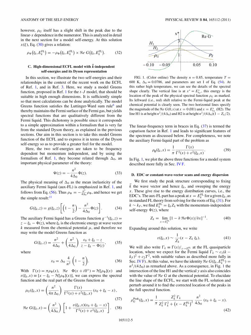
FIG. 1. (Color online) The density n = 0.85, temperature T =600 K, 00 = 0.0786, and parameters are set I of Eq. (54). Atthis rather high temperature, we can see the details of the spectralshape clearly. The vertical line is at x/ = E/

kF, this energy is the

location of the peak of the physical spectral function %G as marked.Its leftward (i.e., red) shift relative to the Fermi-liquid peak at thechemical potential is clearly seen. The two horizontal lines specifythe magnitude of the ,e G(0,x) at x = 0 (H1) and x = E/

kF(H2). The

line H1 is at height n2/(400) and H2 is at height n2/(400)(1 ! Zk/2).

The linear-frequency term in braces in Eq. (37) is termed thecaparison factor in Ref. 1 and leads to significant features ofthe spectrum as discussed below. For completeness, we notethe auxiliary Fermi-liquid part of the problem as

%g(/k,x) = 1-

2(x)22(x) + )2(/k,x)

. (39)

In Fig. 1, we plot the above three functions for a model systemdescribed more fully in Sec. IV F.

D. EDC or constant-wave-vector scans and energy dispersion

We first study the peak structure corresponding to fixing0k the wave vector and hence /k , and sweeping the energyx. These give rise to the energy distribution curves, i.e., theEDC’s. The aux-FL part has a peak at x = EFL

k for a given /k , asin standard FL theory from solving for the roots of Eq. (31). Fork ) kF , we find EFL

k = /kZk with the momentum-independentself-energy #(z), where

Zk = limx'EFL

k

[1 ! 3 ,e#(x)/3x]!1. (40)

Expanding around this solution, we write

)(/k,x) ) 1Zk

(x ! Zk /k). (41)

We will also write 2k . 2(x)/x'EFLk

at the FL quasiparticlelocation, where we expect for the Fermi liquid 2k ) c1(k !kF )2 + c2T

2, with suitable values as described more fully inSec. IV F). At this value, we have the identity ,e G(/k,E

FLk ) =

n2/(400) as remarked above. As a consequence, in Fig. 1 theintersection of the line H1 and the vertical y axis also coincideswith the value of ,e G at the chemical potential. To elucidatethe line shape of the ECFL, we start with the FL solution andperturb around it to find the corrected location of the peaks inthe full spectral function.

%PeakG (/k,x) = 1

-

Z2k 2k

Z2k 22

k +$x ! EFL

k

%2

n2

400()0 + /k ! x).

(42)

165112-5

B. SRIRAM SHASTRY PHYSICAL REVIEW B 84, 165112 (2011)

Peak ratio

uk/10

T=300K

# ( k)Qk

Ek "0.1 "0.05

0.1

0.2

0.3

0.4

0.5

$

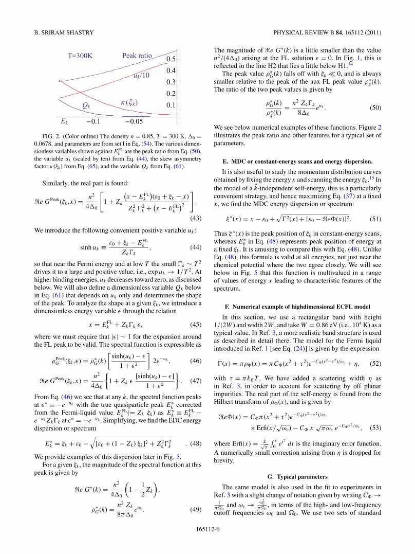
FIG. 2. (Color online) The density n = 0.85, T = 300 K, 00 =0.0678, and parameters are from set I in Eq. (54). The various dimen-sionless variables shown against EFL

k are the peak ratio from Eq. (50),the variable uk (scaled by ten) from Eq. (44), the skew asymmetryfactor 4(/k) from Eq. (65), and the variable Qk from Eq. (61).

Similarly, the real part is found:

,e GPeak(/k,x) = n2

400

0

1 + Zk

$x ! EFL

k

%()0 + /k ! x)

Z2k 22

k +$x ! EFL

k

%2

1

.

(43)

We introduce the following convenient positive variable uk:

sinh uk . )0 + /k ! EFLk

Zk2k

, (44)

so that near the Fermi energy and at low T the small 2k ) T 2

drives it to a large and positive value, i.e., exp uk ' 1/T 2. Athigher binding energies, uk decreases toward zero, as discussedbelow. We will also define a dimensionless variable Qk belowin Eq. (61) that depends on uk only and determines the shapeof the peak. To analyze the shape at a given /k , we introduce adimensionless energy variable 5 through the relation

x = EFLk + Zk2k 5, (45)

where we must require that |5| ) 1 for the expansion aroundthe FL peak to be valid. The spectral function is expressible as

%PeakG (/k,5) = %/

G(k)*

sinh(uk) ! 5

1 + 52

+2e!uk , (46)

,e GPeak(/k,x) = n2

400

21 + Zk 5

[sinh(uk) ! 5]1 + 52

3. (47)

From Eq. (46) we see that at any k, the spectral function peaksat 5/ . !e!uk with the true quasiparticle peak E/

k correctedfrom the Fermi-liquid value EFL

k (= Zk /k) as E/k . EFL

k !e!ukZk2k at 5/ = !e!uk . Simplifying, we find the EDC energydispersion or spectrum

E/k = /k + )0 !

4[)0 + (1 ! Zk) /k]2 + Z2

k22k . (48)

We provide examples of this dispersion later in Fig. 5.For a given /k , the magnitude of the spectral function at this

peak is given by

,e G/(k) = n2

400

.1 ! 1

2Zk

/,

%/G(k) = n2 Zk

8-00euk . (49)

The magnitude of ,e G/(k) is a little smaller than the valuen2/(400) arising at the FL solution 5 = 0. In Fig. 1, this isreflected in the line H2 that lies a little below H1.14

The peak value %/G(k) falls off with /k 1 0, and is always

smaller relative to the peak of the aux-FL peak value %/g (k).

The ratio of the two peak values is given by

%/G(k)

%/g (k)

= n2 Zk2k

800euk . (50)

We see below numerical examples of these functions. Figure 2illustrates the peak ratio and other features for a typical set ofparameters.

E. MDC or constant-energy scans and energy dispersion.

It is also useful to study the momentum distribution curvesobtained by fixing the energy x and scanning the energy /k .15 Inthe model of a 0k-independent self-energy, this is a particularlyconvenient strategy, and hence maximizing Eq. (37) at a fixedx, we find the MDC energy dispersion or spectrum:

/ /(x) = x ! )0 +5

22(x) + [)0 ! ,e#(x)]2. (51)

Thus / /(x) is the peak position of /k in constant-energy scans,whereas E/

k in Eq. (48) represents peak position of energy ata fixed /k . It is amusing to compare this with Eq. (48). UnlikeEq. (48), this formula is valid at all energies, not just near thechemical potential where the two agree closely. We will seebelow in Fig. 5 that this function is multivalued in a rangeof values of energy x leading to characteristic features of thespectrum.

F. Numerical example of highdimensional ECFL model

In this section, we use a rectangular band with height1/(2W ) and width 2W , and take W = 0.86 eV (i.e., 104 K) as atypical value. In Ref. 3, a more realistic band structure is usedas described in detail there. The model for the Fermi liquidintroduced in Ref. 1 [see Eq. (24)] is given by the expression

2(x) = -%#(x) = -C#(x2 + 6 2)e!C#(x2+6 2)/.c + 1, (52)

with 6 = -kBT . We have added a scattering width 1 asin Ref. 3, in order to account for scattering by off planarimpurities. The real part of the self-energy is found from theHilbert transform of %#(x), and is given by

,e#(x) = C#- (x2 + 6 2)e!C#(x2+6 2)/.c

- Erfi(x/2

.c) ! C# x2

-.c e!C#6 2/.c , (53)

where Erfi(x) = 22-

6 x

0 et2dt is the imaginary error function.

A numerically small correction arising from 1 is dropped forbrevity.

G. Typical parameters

The same model is also used in the fit to experiments inRef. 3 with a slight change of notation given by writing C# '

1-70

and .c ' .20

-70, in terms of the high- and low-frequency

cutoff frequencies .0 and 70. We use two sets of standard

165112-6

ANATOMY OF THE SELF-ENERGY PHYSICAL REVIEW B 84, 165112 (2011)

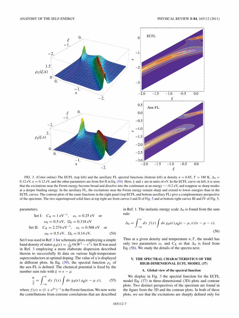
FIG. 3. (Color online) The ECFL (top left) and the auxiliary FL spectral functions (bottom left) at density n = 0.85, T = 180 K, 00 =0.12 eV, 1 = 0.12 eV, and the other parameters are from Set II in Eq. (54). Here, / and x are in units of eV. In the ECFL curve on left, it is seenthat the excitations near the Fermi energy become broad and dissolve into the continuum at an energy )!0.2 eV, and reappear as sharp modesat a deeper binding energy. In the auxiliary FL, the excitations near the Fermi energy remain sharp and extend to lower energies than in theECFL curves. The contour plots of the same functions in the right panel (top ECFL and bottom auxiliary FL) give a complementary perspectiveof the spectrum. The two superimposed solid lines at top right are from curves I and II of Fig. 5 and at bottom right curves III and IV of Fig. 5.

parameters;

Set I: C# = 1 eV!1, .c = 0.25 eV or

.0 = 0.5 eV, 70 = 0.318 eV

Set II: C# = 2.274 eV!1, .c = 0.568 eV or

.0 = 0.5 eV, 70 = 0.14 eV. (54)

Set I was used in Ref. 1 for schematic plots employing a simpleband density of states gB ()) = 1

2W8(W 2 ! )2). Set II was used

in Ref. 3 employing a more elaborate dispersion describedtherein to successfully fit data on various high-temperaturesuperconductors at optimal doping. The value of 1 is displayedin different plots. In Eq. (39), the spectral function %g ofthe aux-FL is defined. The chemical potential is fixed by thenumber sum rule with / = 5 ! µ

n

2=

! $

!$dx f (x)

!d5 gB(5) %g(5 ! µ,x), (55)

where f (x) = (1 + e'x)!1 is the Fermi function. We now writethe contributions from extreme correlations that are described

in Ref. 1. The inelastic energy scale 00 is found from the sumrule:

00 =! $

!$dx f (x)

!d5 gB(5) %g(5 ! µ,x) (5 ! µ ! x).

(56)

Thus at a given density and temperature n,T , the model hasonly two parameters .c and C# so that 00 is fixed fromEq. (56). We study the details of the spectra next.

V. THE SPECTRAL CHARACTERISTICS OF THEHIGH-DIMENSIONAL ECFL MODEL (37)

A. Global view of the spectral function

We display in Fig. 3 the spectral function for the ECFLmodel Eq. (37) in three-dimensional (3D) plots and contourplots. Two distinct perspectives of the spectrum are found inthe figure from the 3D and the contour plots. In both of theseplots, we see that the excitations are sharply defined only for

165112-7

B. SRIRAM SHASTRY PHYSICAL REVIEW B 84, 165112 (2011)

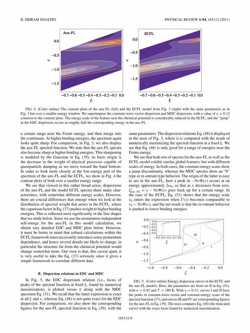
FIG. 4. (Color online) The contour plots of the aux-FL (left) and the ECFL model from Fig. 3 (right) with the same parameters as inFig. 3 but over a smaller energy window. We superimpose the constant-wave-vector dispersion and MDC dispersion, with a value of 1 = 0.12common to the contour plots. The energy scale of the feature near the chemical potential is considerably reduced in the ECFL, and the “jump”in the EDC dispersion occurs at roughly half the corresponding energy in the aux-FL.

a certain range near the Fermi energy, and then merge intothe continuum. At higher binding energies, the spectrum againlooks quite sharp. For comparison, in Fig. 3, we also displaythe aux-FL spectral function. We note that the aux-FL spectraalso become sharp at higher binding energies. This sharpeningis modeled by the Gaussian in Eq. (39), its basic origin isthe decrease in the weight of physical processes capable ofquasiparticle damping as we move toward the band bottom.In order to look more closely at the low-energy part of thespectrum of the aux-FL and the ECFL, we show in Fig. 4 thecontour plots of both over a smaller energy range.

We see that viewed in this rather broad sense, dispersionsof the aux-FL and the model ECFL spectra share many char-acteristics, with somewhat different energy scales. However,there are crucial differences that emerge when we look at thedistribution of spectral weight that arises in the ECFL, wherethe caparison factor in Eq. (37) pushes weight to higher bindingenergies. This is reflected most significantly in the line shapesthat we study below. Since we use the momentum-independentself-energy for the aux-FL in this model calculation, weobtain very detailed EDC and MDC plots below. However,it must be borne in mind that refined calculations within theECFL framework must necessarily introduce some momentumdependence, and hence several details are likely to change, inparticular the structure far from the chemical potential wouldchange somewhat more. Our view is that, this caveat apart, itis very useful to take the Eq. (37) seriously since it gives asimple framework to correlate different data.

B. Dispersion relations in EDC and MDC

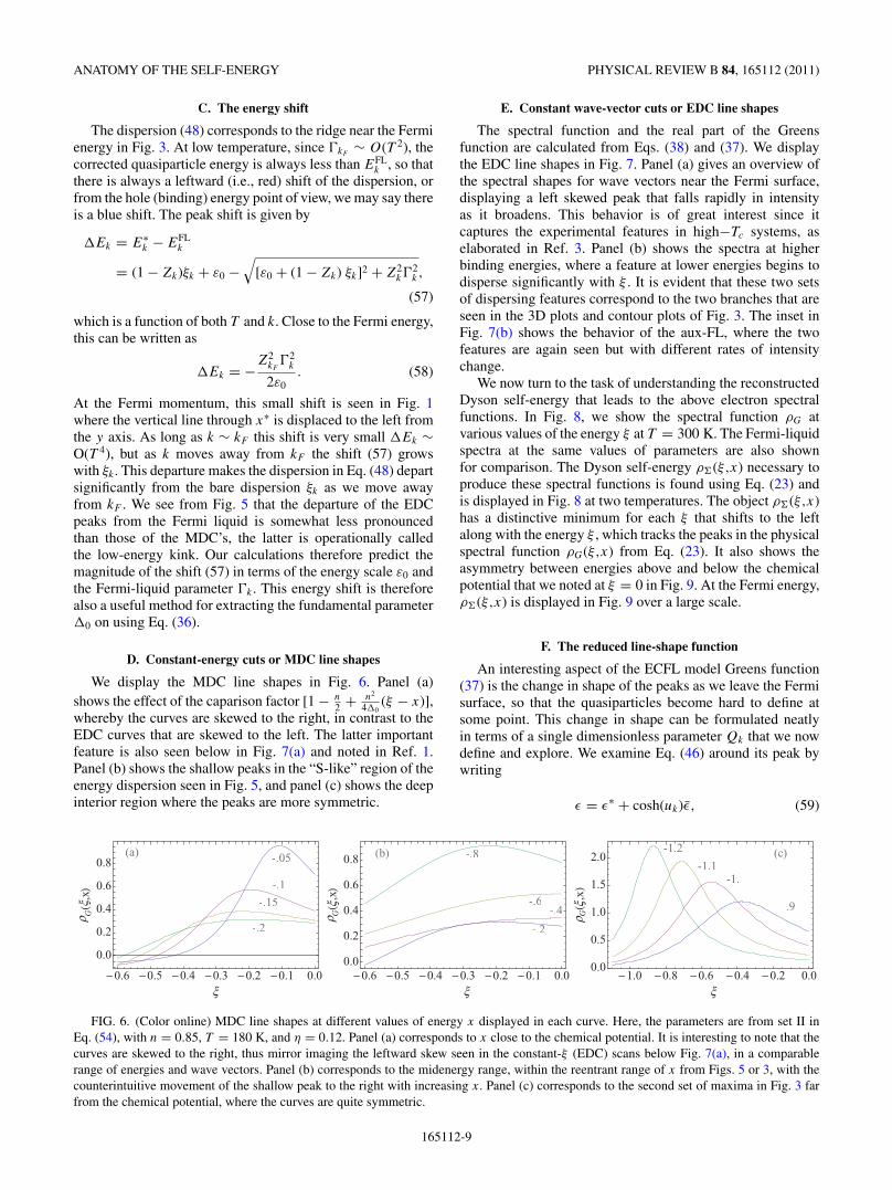
In Fig. 5, the EDC dispersion relation (i.e., locus ofpeaks of the spectral function at fixed / , found by numericalmaximization), is plotted versus / along with the MDCspectrum Eq. (51). We recall that the latter expression is exactat all / and x, whereas Eq. (48) is not quite exact for the EDCdispersion. For comparison, we also show the correspondingfigures for the aux-FL spectral function in Eq. (39), with the

same parameters. The dispersion relations Eq. (48) is displayedin the inset of Fig. 5, where it is compared with the result ofnumerically maximizing the spectral function at a fixed / . Wesee that Eq. (48) is only good for a range of energies near theFermi energy.

We see that both sets of spectra for the aux-FL as well as theECFL model exhibit similar global features, but with differentscales of energy. In both cases, the constant energy scans showa jump discontinuity, whereas the MDC spectra show an “S”type or re-entrant type behavior. The origin of the latter is easyto see in the aux-FL, here a peak in !,e#(x) occurs at anenergy approximately 2.0, so that as x decreases from zero,/ /

aux!FL = x ! ,e#(x) goes back up for a certain range. Inthe case of the ECFL, Eq. (51) shows that the energy scale)0 enters the expression when 2(x) becomes comparable to)0 ! ,e#(x), and the net result is that the re-entrant behavioris pushed to lower binding energies.

0.4 0.3 0.2 0.1 0.0

0.80.60.40.20.0

III

III

IV$

"1.0 "0.8 "0.6 "0.4 "0.2 0.0

"1.2

"1.0

"0.8

"0.6

"0.4

" """"

" " " "

0.2

0.0

$

x

FIG. 5. (Color online) Energy dispersion curves in the ECFL andthe aux-FL models. Here, the parameters are from set II in Eq. (54),with n = 0.85 and T = 180 K. With 1 = 0.12, curves I and II havethe peaks in constant-wave-vector and constant-energy scans of thespectral function (37), and curves III and IV are corresponding figuresfor the aux-FL in Eq. (39). The inset compares Eq. (48) (the truncatedcurve) with the exact locus found by numerical maximization.

165112-8

ANATOMY OF THE SELF-ENERGY PHYSICAL REVIEW B 84, 165112 (2011)

C. The energy shift

The dispersion (48) corresponds to the ridge near the Fermienergy in Fig. 3. At low temperature, since 2kF

) O(T 2), thecorrected quasiparticle energy is always less than EFL

k , so thatthere is always a leftward (i.e., red) shift of the dispersion, orfrom the hole (binding) energy point of view, we may say thereis a blue shift. The peak shift is given by

0Ek = E/k ! EFL

k

= (1 ! Zk)/k + )0 !4

[)0 + (1 ! Zk) /k]2 + Z2k2

2k ,

(57)

which is a function of both T and k. Close to the Fermi energy,this can be written as

0Ek = !Z2

kF22

k

2)0. (58)

At the Fermi momentum, this small shift is seen in Fig. 1where the vertical line through x/ is displaced to the left fromthe y axis. As long as k ) kF this shift is very small 0Ek )O(T 4), but as k moves away from kF the shift (57) growswith /k . This departure makes the dispersion in Eq. (48) departsignificantly from the bare dispersion /k as we move awayfrom kF . We see from Fig. 5 that the departure of the EDCpeaks from the Fermi liquid is somewhat less pronouncedthan those of the MDC’s, the latter is operationally calledthe low-energy kink. Our calculations therefore predict themagnitude of the shift (57) in terms of the energy scale )0 andthe Fermi-liquid parameter 2k . This energy shift is thereforealso a useful method for extracting the fundamental parameter00 on using Eq. (36).

D. Constant-energy cuts or MDC line shapes

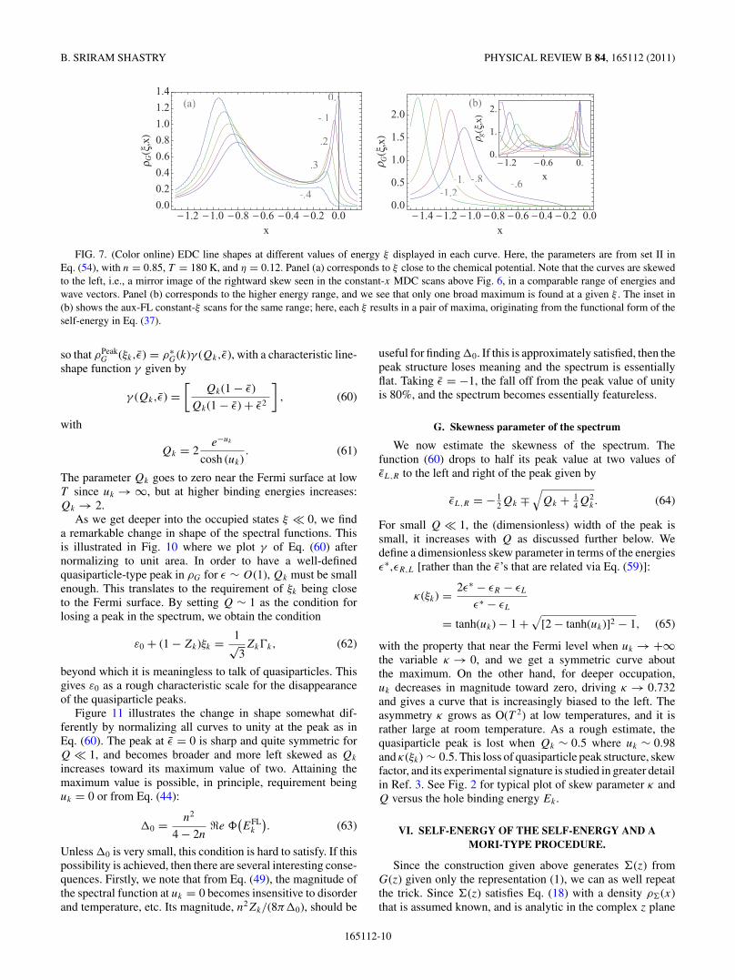
We display the MDC line shapes in Fig. 6. Panel (a)shows the effect of the caparison factor [1 ! n

2 + n2

400(/ ! x)],

whereby the curves are skewed to the right, in contrast to theEDC curves that are skewed to the left. The latter importantfeature is also seen below in Fig. 7(a) and noted in Ref. 1.Panel (b) shows the shallow peaks in the “S-like” region of theenergy dispersion seen in Fig. 5, and panel (c) shows the deepinterior region where the peaks are more symmetric.

E. Constant wave-vector cuts or EDC line shapes

The spectral function and the real part of the Greensfunction are calculated from Eqs. (38) and (37). We displaythe EDC line shapes in Fig. 7. Panel (a) gives an overview ofthe spectral shapes for wave vectors near the Fermi surface,displaying a left skewed peak that falls rapidly in intensityas it broadens. This behavior is of great interest since itcaptures the experimental features in high!Tc systems, aselaborated in Ref. 3. Panel (b) shows the spectra at higherbinding energies, where a feature at lower energies begins todisperse significantly with / . It is evident that these two setsof dispersing features correspond to the two branches that areseen in the 3D plots and contour plots of Fig. 3. The inset inFig. 7(b) shows the behavior of the aux-FL, where the twofeatures are again seen but with different rates of intensitychange.

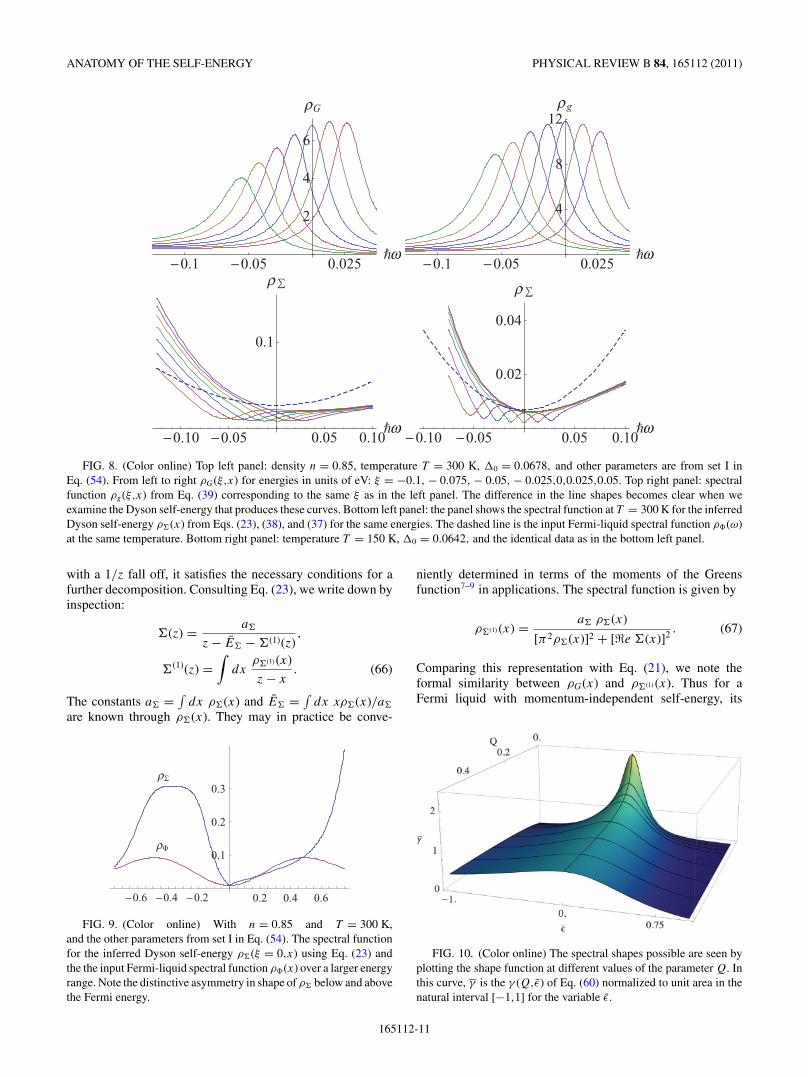
We now turn to the task of understanding the reconstructedDyson self-energy that leads to the above electron spectralfunctions. In Fig. 8, we show the spectral function %G atvarious values of the energy / at T = 300 K. The Fermi-liquidspectra at the same values of parameters are also shownfor comparison. The Dyson self-energy %!(/,x) necessary toproduce these spectral functions is found using Eq. (23) andis displayed in Fig. 8 at two temperatures. The object %!(/,x)has a distinctive minimum for each / that shifts to the leftalong with the energy / , which tracks the peaks in the physicalspectral function %G(/,x) from Eq. (23). It also shows theasymmetry between energies above and below the chemicalpotential that we noted at / = 0 in Fig. 9. At the Fermi energy,%!(/,x) is displayed in Fig. 9 over a large scale.

F. The reduced line-shape function

An interesting aspect of the ECFL model Greens function(37) is the change in shape of the peaks as we leave the Fermisurface, so that the quasiparticles become hard to define atsome point. This change in shape can be formulated neatlyin terms of a single dimensionless parameter Qk that we nowdefine and explore. We examine Eq. (46) around its peak bywriting

5 = 5/ + cosh(uk)5, (59)

(a) -.05

-.1

-.2

-.15

0.6 0.5 0.4 0.3 0.2 0.1 0.0

0.0

0.2

0.4

0.6

0.8

$ $ $

G$ ,

x

(b) -.8

-.6-.4

-.2

0.6 0.5 0.4 0.3 0.2 0.1 0.00.0

0.2

0.4

0.6

0.8

G,x

-.9

-1.-1.1

-1.2 (c)

1.0 0.8 0.6 0.4 0.2 0.00.0

0.5

1.0

1.5

2.0

! G,x$ $

!!

FIG. 6. (Color online) MDC line shapes at different values of energy x displayed in each curve. Here, the parameters are from set II inEq. (54), with n = 0.85, T = 180 K, and 1 = 0.12. Panel (a) corresponds to x close to the chemical potential. It is interesting to note that thecurves are skewed to the right, thus mirror imaging the leftward skew seen in the constant-/ (EDC) scans below Fig. 7(a), in a comparablerange of energies and wave vectors. Panel (b) corresponds to the midenergy range, within the reentrant range of x from Figs. 5 or 3, with thecounterintuitive movement of the shallow peak to the right with increasing x. Panel (c) corresponds to the second set of maxima in Fig. 3 farfrom the chemical potential, where the curves are quite symmetric.

165112-9

B. SRIRAM SHASTRY PHYSICAL REVIEW B 84, 165112 (2011)

(a) 0.

-.1

-.2

-.3

-.4

1.2 1.0 0.8 0.6 0.4 0.2 0.00.0

0.2

0.4

0.6

0.8

1.0

1.2

1.4

x

! G$,

x

(b)

-.6-.8-1.-1.2

1.2 0.6 0.0.

1.

2.

x

! g$,

x

1.4 1.2 1.0 0.8 0.6 0.4 0.2 0.00.0

0.5

1.0

1.5

2.0

x

! G$,

x

FIG. 7. (Color online) EDC line shapes at different values of energy / displayed in each curve. Here, the parameters are from set II inEq. (54), with n = 0.85, T = 180 K, and 1 = 0.12. Panel (a) corresponds to / close to the chemical potential. Note that the curves are skewedto the left, i.e., a mirror image of the rightward skew seen in the constant-x MDC scans above Fig. 6, in a comparable range of energies andwave vectors. Panel (b) corresponds to the higher energy range, and we see that only one broad maximum is found at a given / . The inset in(b) shows the aux-FL constant-/ scans for the same range; here, each / results in a pair of maxima, originating from the functional form of theself-energy in Eq. (37).

so that %PeakG (/k,5) = %/

G(k)* (Qk,5), with a characteristic line-shape function * given by

* (Qk,5) =*

Qk(1 ! 5)Qk(1 ! 5) + 52

+, (60)

with

Qk = 2e!uk

cosh (uk). (61)

The parameter Qk goes to zero near the Fermi surface at lowT since uk ' $, but at higher binding energies increases:Qk ' 2.

As we get deeper into the occupied states / 1 0, we finda remarkable change in shape of the spectral functions. Thisis illustrated in Fig. 10 where we plot * of Eq. (60) afternormalizing to unit area. In order to have a well-definedquasiparticle-type peak in %G for 5 ) O(1), Qk must be smallenough. This translates to the requirement of /k being closeto the Fermi surface. By setting Q ) 1 as the condition forlosing a peak in the spectrum, we obtain the condition

)0 + (1 ! Zk)/k = 123Zk2k, (62)

beyond which it is meaningless to talk of quasiparticles. Thisgives )0 as a rough characteristic scale for the disappearanceof the quasiparticle peaks.

Figure 11 illustrates the change in shape somewhat dif-ferently by normalizing all curves to unity at the peak as inEq. (60). The peak at 5 = 0 is sharp and quite symmetric forQ 1 1, and becomes broader and more left skewed as Qk

increases toward its maximum value of two. Attaining themaximum value is possible, in principle, requirement beinguk = 0 or from Eq. (44):

00 = n2

4 ! 2n,e #

$EFL

k

%. (63)

Unless 00 is very small, this condition is hard to satisfy. If thispossibility is achieved, then there are several interesting conse-quences. Firstly, we note that from Eq. (49), the magnitude ofthe spectral function at uk = 0 becomes insensitive to disorderand temperature, etc. Its magnitude, n2Zk/(8-00), should be

useful for finding 00. If this is approximately satisfied, then thepeak structure loses meaning and the spectrum is essentiallyflat. Taking 5 = !1, the fall off from the peak value of unityis 80%, and the spectrum becomes essentially featureless.

G. Skewness parameter of the spectrum

We now estimate the skewness of the spectrum. Thefunction (60) drops to half its peak value at two values of5L,R to the left and right of the peak given by

5L,R = ! 12Qk *

4Qk + 1

4Q2k. (64)

For small Q 1 1, the (dimensionless) width of the peak issmall, it increases with Q as discussed further below. Wedefine a dimensionless skew parameter in terms of the energies5/,5R,L [rather than the 5’s that are related via Eq. (59)]:

4(/k) = 25/ ! 5R ! 5L

5/ ! 5L

= tanh(uk) ! 1 +5

[2 ! tanh(uk)]2 ! 1, (65)

with the property that near the Fermi level when uk ' +$the variable 4 ' 0, and we get a symmetric curve aboutthe maximum. On the other hand, for deeper occupation,uk decreases in magnitude toward zero, driving 4 ' 0.732and gives a curve that is increasingly biased to the left. Theasymmetry 4 grows as O(T 2) at low temperatures, and it israther large at room temperature. As a rough estimate, thequasiparticle peak is lost when Qk ) 0.5 where uk ) 0.98and 4(/k) ) 0.5. This loss of quasiparticle peak structure, skewfactor, and its experimental signature is studied in greater detailin Ref. 3. See Fig. 2 for typical plot of skew parameter 4 andQ versus the hole binding energy Ek .

VI. SELF-ENERGY OF THE SELF-ENERGY AND AMORI-TYPE PROCEDURE.

Since the construction given above generates !(z) fromG(z) given only the representation (1), we can as well repeatthe trick. Since !(z) satisfies Eq. (18) with a density %!(x)that is assumed known, and is analytic in the complex z plane

165112-10

ANATOMY OF THE SELF-ENERGY PHYSICAL REVIEW B 84, 165112 (2011)

0.1 0.05 0.025%

2

4

6

!G

0.1 0.05 0.025%

4

8

12g

0.10 0.05 0.05 0.10%

0.1

0.10 0.05 0.05 0.10%

0.02

0.04

!

!!

FIG. 8. (Color online) Top left panel: density n = 0.85, temperature T = 300 K, 00 = 0.0678, and other parameters are from set I inEq. (54). From left to right %G(/,x) for energies in units of eV: / = !0.1, ! 0.075, ! 0.05, ! 0.025,0,0.025,0.05. Top right panel: spectralfunction %g(/,x) from Eq. (39) corresponding to the same / as in the left panel. The difference in the line shapes becomes clear when weexamine the Dyson self-energy that produces these curves. Bottom left panel: the panel shows the spectral function at T = 300 K for the inferredDyson self-energy %!(x) from Eqs. (23), (38), and (37) for the same energies. The dashed line is the input Fermi-liquid spectral function %#(.)at the same temperature. Bottom right panel: temperature T = 150 K, 00 = 0.0642, and the identical data as in the bottom left panel.

with a 1/z fall off, it satisfies the necessary conditions for afurther decomposition. Consulting Eq. (23), we write down byinspection:

!(z) = a!

z ! E! ! !(1)(z),

!(1)(z) =!

dx%!(1) (x)z ! x

. (66)

The constants a! =6

dx %!(x) and E! =6

dx x%!(x)/a!

are known through %!(x). They may in practice be conve-

!

!

0.6 0.4 0.2 0.2 0.4 0.6

0.1

0.2

0.3

FIG. 9. (Color online) With n = 0.85 and T = 300 K,and the other parameters from set I in Eq. (54). The spectral functionfor the inferred Dyson self-energy %!(/ = 0,x) using Eq. (23) andthe the input Fermi-liquid spectral function %#(x) over a larger energyrange. Note the distinctive asymmetry in shape of %! below and abovethe Fermi energy.

niently determined in terms of the moments of the Greensfunction7–9 in applications. The spectral function is given by

%!(1) (x) = a! %!(x)

[-2%!(x)]2 + [,e !(x)]2 . (67)

Comparing this representation with Eq. (21), we note theformal similarity between %G(x) and %!(1) (x). Thus for aFermi liquid with momentum-independent self-energy, its

FIG. 10. (Color online) The spectral shapes possible are seen byplotting the shape function at different values of the parameter Q. Inthis curve, * is the * (Q,5) of Eq. (60) normalized to unit area in thenatural interval [!1,1] for the variable 5.

165112-11

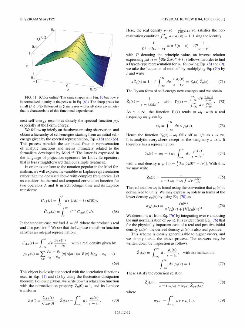
B. SRIRAM SHASTRY PHYSICAL REVIEW B 84, 165112 (2011)

FIG. 11. (Color online) The same shapes as in Fig. 10 but now *

is normalized to unity at the peak as in Eq. (60). The sharp peaks forsmall Q ! 0.25 flatten out as Q increases with a left skew asymmetrythat is characteristic of this functional dependence.

next self-energy resembles closely the spectral function %G,especially at the Fermi energy.

We follow up briefly on the above amusing observation, andobtain a hierarchy of self-energies starting from an initial self-energy given by the spectral representation, Eqs. (18) and (66).This process parallels the continued fraction representationof analytic functions and seems intimately related to theformalism developed by Mori.7,8 The latter is expressed inthe language of projection operators for Liouville operatorsthat is less straightforward than our simple treatment.

In order to conform to the notation popular in the Mori for-malism, we will express the variables in Laplace representationrather than the one used above with complex frequencies. Letus consider the thermal and temporal correlation function fortwo operators A and B in Schrodinger time and its Laplacetransform:

CAB(t) =! '

0d6 %A(t ! i6 )B(0)&,

CAB(s) =! $

0e!st CAB(t) dt. (68)

In the standard case, we find A = B†, where the product is realand also positive.16 We see that the Laplace-transform functionsatisfies an integral representation:

CAB(s) =! $

!$d9

%AB(9)s ! i9

, with a real density given by

%AB(9) ="

nm

pm ! pn

)n ! )m

%n|A|m& %m|B|n& (()n ! )m ! 9).

(69)

This object is closely connected with the correlation functionsused in Eqs. (1) and (2) by using the fluctuation-dissipationtheorem. Following Mori, we write down a relaxation functionwith the normalization property Z0(0) = 1, and its Laplacetransform

Z0(t) . CAB(t)CAB(0)

, Z0(s) =! $

!$d9

%0(9)s ! i9

. (70)

Here, the real density %0(9) = 1C(0)%AB(9), satisfies the nor-

malization condition6 $!$ d9 %0(9) = 1. Using the identity

10+ + i(u ! v)

= - ((u ! v) ! iP1

u ! v,

with P denoting the principle value, an inverse relationexpressing %0(9) = 1

-,e Z0(0+ + i9) follows. In order to find

a Dyson-type representation for %0, following Eqs. (8) and (9),we take the “equation of motion” by multiplying Eq. (70) bys and write

sZ0(s) = 1 + i

! $

!$d9

9 %0(9)s ! i9

. Y0(s) Z0(s). (71)

The Dyson form of self-energy now emerges and we obtain

Z0(s) = 1s ! iY0(s)

, with Y0(s) =6 $!$ d9 9 %0(9)

s!i96 $!$ d9 %0(9)

s!i9

. (72)

As s ' $, the function Y0(s) tends to .1, with a realfrequency .1 given by

.1 =! $

!$d9 9 %0(9). (73)

Hence the function Y0(s) ! .1 falls off as 1/s as s ' $.It is analytic everywhere except on the imaginary s axis. Ittherefore has a representation

Y0(s) ! .1 = i &1

! $

!$d9

%1(9)s ! i9

, (74)

with a real density &1%1(9) = 1-+m[Y0(0+ + i9)]. With this,

we may write

Z0(s) = 1

s ! i .1 + &16

d9 %1(9)s!i9

. (75)

The real number &1 is found using the convention that %1(9) isnormalized to unity. We may express %1 solely in terms of thelower density %0(9) by using Eq. (70) as

&1%1(u) = %0(u)

-2%20 (u) + [H[%0](u)]2 . (76)

We determine &1 from Eq. (76) by integrating over 9 and usingthe unit normalization of %1(u). It is evident from Eq. (76) thatfor the physically important case of a real and positive initialdensity %0(9), the derived density %1(9) is also real positive.

This scheme is clearly generalizable to higher orders, andwe simply iterate the above process. The answers may bewritten down by inspection as follows:

Zj (s) =! $

!$d9

%j (9)s ! i9

, with normalization:! $

!$d9 %j (9) = 1. (77)

These satisfy the recursion relation

Zj (s) = 1

s ! i .j+1 + &j+1 Zj+1(s), (78)

where

.j+1 =! $

!$d9 9 %j (9), (79)

165112-12

ANATOMY OF THE SELF-ENERGY PHYSICAL REVIEW B 84, 165112 (2011)

and &j+1 as well as %j+1(9) are defined through

&j+1 %j+1(u) = %j (u)-2 %2

j (u) + [H[%j ](u)]2. (80)

Note that the numbers &j as well as .j are real, and for all j ,the densities %j (9) are positive provided the the initial density%o(9) is positive. This situation arises when the initial operatorsB = A†, as mentioned above.

It is clear that Eq. (76) is the precise analog of the rela-tion (23) for the Greens function. The hierarchy of equationsconsisting of Eqs. (45)–(49) constitutes an iteration schemethat starts with the j = 0 correlation function in Eq. (70). Thisis a forward hierarchy in the sense that successive densitiesat level j + 1 are expressed explicitly in terms of the earlierones at level j . In the reverse direction, it is rather simplersince level j is explicitly given in terms of level j + 1 byEq. (78). The use of this set of equations requires some apriori knowledge of the behavior of higher order self-energiesto deduce the lower ones. Standard approximations7 consist ofeither truncation of the series or making a physical assumptionsuch as a Gaussian behavior at some level and then workingout the lower level objects. Our object in presenting the aboveprocedure is merely to point out that this iterative scheme is in

essence a rather simple application of the self-energy conceptdescribed above, with the repeated use of Eq. (23).

VII. SUMMARY AND CONCLUSIONS

A new form of the electronic Greens function, departingwidely from the Dyson form arises in the extreme correlationtheory of the t-J model. Motivated by its considerablesuccess in explaining ARPES data of optimally doped cupratesuperconductors,3 we have presented in this paper results onthe detailed structure of this Greens function and its spectralfunction. An illustrative example is provided, complete withnumerical results, so that the novel line shape and itsdependence on parameters is revealed. We have also presenteda set of explicit results on the Mori form of the self-energy thatholds promise in several contexts.

ACKNOWLEDGMENTS

This work was supported by DOE under Grant No. FG02-06ER46319. I thank G-H. Gweon for helpful comments andvaluable discussions. I thank A. Dhar and P. Wolfle for usefulcomments regarding the Mori formalism.

1B. S. Shastry, Phys. Rev. Lett. 107, 056403 (2011).2B. S. Shastry, Phys. Rev. B 81, 045121 (2010).3G.-H. Gweon, B. S. Shastry, and G. D. Gu, Phys. Rev. Lett. 107,056404 (2011).

4D. E. Logan, M. P. Eastwood and M. A. Tusch, J. Phys. Condens.Matter 10, 2673 (1998).

5Z. Wang, Y. Bang, and G. Kotliar, Phys. Rev. Lett. 67, 2733 (1991).6J. M. Luttinger and J. C. Ward, Phys. Rev 118, 1417 (1960); J. M.Luttinger, ibid. 119, 1153 (1960); 121, 942 (1961).

7H. Mori, Prog. Theor. Phys. 33, 423 (1965); 34, 399 (1965).8M. Dupuis, Prog. Theor. Phys. 37, 502 (1967).9J. J. Deisz, D. W. Hess, and J. W. Serene, Phys. Rev. 55, 2089(1997).

10A. A. Abrikosov, L. Gorkov, and I. Dzyaloshinski, Methodsof Quantum Field Theory in Statistical Physics (Prentice-Hall,Englewood Cliffs, NJ, 1963). Our %G(/k,x) corresponds to thecombination of spectral functions A(0k,x) and B(0k,x) used here.

11The positive part constraint on the right of the following equationcan be often omitted, we found that it is violated very slightly )3%in many cases. We omit it for simplicity in the following.

12Shifting E by a constant is also possible but the optimal choice isthe one made here.

13The notation is simplified from that in Ref. 1 by calling theextremely correlated Greens function as G rather than G and theoverbar in the self-energy # is omitted.

14At T = 0, this finite value persists and ,eGPeak[/k,x/(/k)] does not

diverge, so that one might be concerned that the Luttinger-Wardvolume theorem is being disobeyed. In comparison, note that thestandard FL Greens function behaves in a slightly different way,at any finite T and /k , at the energy x = EFL

k we find both a peakin the spectral function %g(/k,E

FLk ) and a zero of the ,eg(/k,E

FLk ),

whereas at T = 0, we find a delta peak in the spectral function%g(/k,E

FLk ) and a pole of the ,eg(/k,E

FLk ). However we see that the

FL divergence of the real part of G of a typical Fermi liquid doesoccur, but displaced by a very small energy scale O(T 4). The peakpositions are displayed in Fig. 1 at a high enough temperature sothat the features are distinguishable.

15The process of scanning /k used here differs slightly from the trueMDC’s, where one scans the wave vector 0k rather than the energy/k , but is more convenient here.

16The spectral function %AA† (x) defined below in Eq. (69) is positiveas well. However, that condition can be relaxed and we can dowith less, provided that the spectral function in Eq. (69) is real(rather than positive). For this to happen, we may allow for A 3= B†,but in this case, assume that both the matrix elements %nAm& and%mBn& are real numbers or imaginary numbers so that the product isreal. These conditions correspond to both operators A and B beingHermitian (or anti Hermitian), and the absence of magnetic fieldsso that the wave functions may be chosen to be real. Thus we willassume the reality of the product of the matrix elements.

165112-13

PHYSICAL REVIEW B 86, 079911(E) (2012)

Erratum: Anatomy of the self-energy [Phys. Rev. B 84, 165112 (2011)]

B. Sriram Shastry(Received 2 August 2012; published 13 August 2012)

DOI: 10.1103/PhysRevB.86.079911 PACS number(s): 79.60.!i, 99.10.Cd

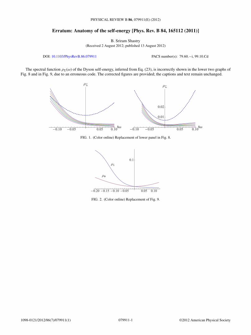
The spectral function !"(#) of the Dyson self-energy, inferred from Eq. (23), is incorrectly shown in the lower two graphs ofFig. 8 and in Fig. 9, due to an erroneous code. The corrected figures are provided; the captions and text remain unchanged.

!

"

!

"

FIG. 1. (Color online) Replacement of lower panel in Fig. 8.

"

"

FIG. 2. (Color online) Replacement of Fig. 9.

079911-11098-0121/2012/86(7)/079911(1) ©2012 American Physical Society