Business AnalyticsADM2302 B / ADM2302 C

Week 2aLinear Programming: Graphical Method I

Notes

• Deferred exams• Student Service Centre (DMS110)• http://www.telfer.uottawa.ca/bcom/en/current-students/55-exams

• Assignment 1• Individual Assignment• Due before class September 29th

• Electronic and Hardcopy

• Lecture Slides Upload• TA DGDs and Office Hours

Graphical Solution Method

• Graphical methods provide visualization of how a solution for a linear programming problem is obtained.

• Please note that Graphical solution is limited to linear programming models containing only two decision variables.

• Decision Variables are axes – decision space• Constraints and Objective Function are lines

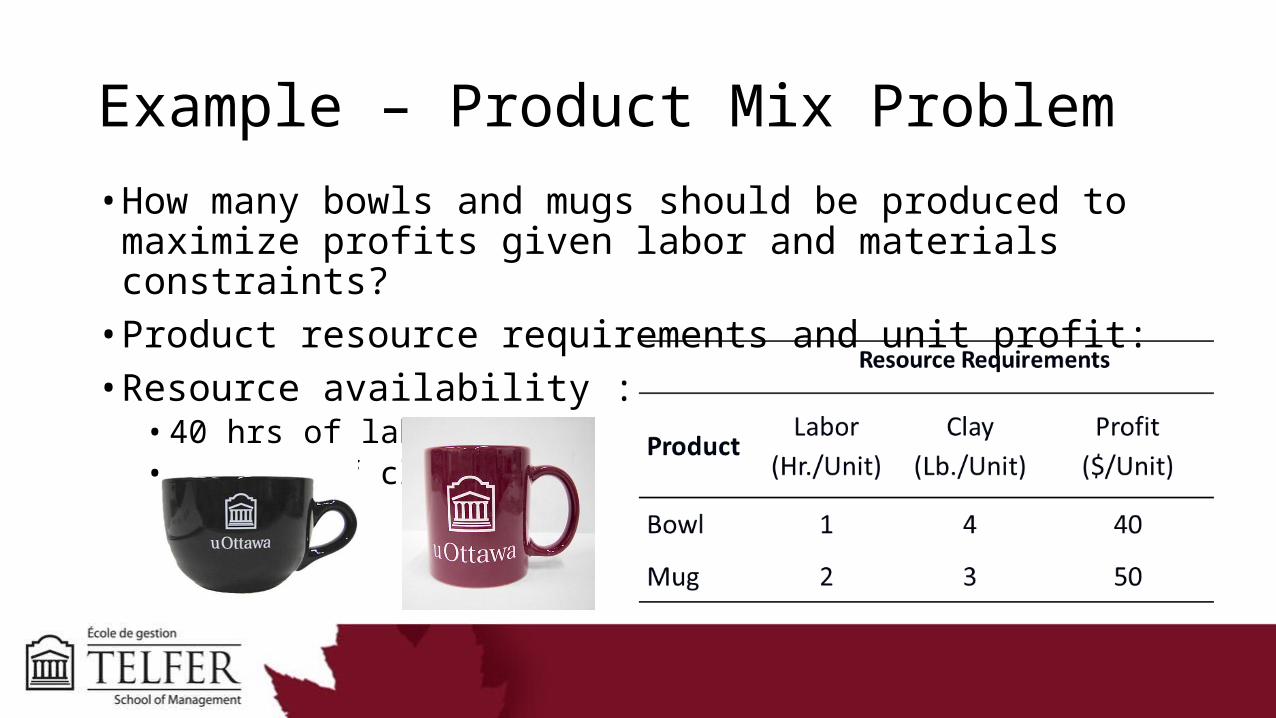
Example – Product Mix Problem

• How many bowls and mugs should be produced to maximize profits given labor and materials constraints?

• Product resource requirements and unit profit:• Resource availability :

• 40 hrs of labor/day• 120 lbs of clay

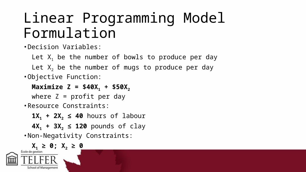
Linear Programming Model Formulation• Decision Variables:

Let X1 be the number of bowls to produce per day

Let X2 be the number of mugs to produce per day • Objective Function:

Maximize Z = $40X1 + $50X2

where Z = profit per day• Resource Constraints:

1X1 + 2X2 ≤ 40 hours of labour

4X1 + 3X2 ≤ 120 pounds of clay• Non-Negativity Constraints:

X1 ≥ 0; X2 ≥ 0

Graphical Solution (1 of 11)

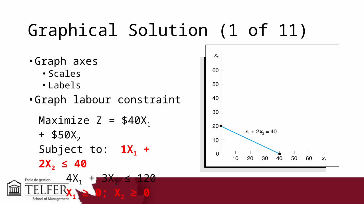
• Graph axes• Scales• Labels

• Graph labour constraint

Maximize Z = $40X1 + $50X2

Subject to: 1X1 + 2X2 ≤ 404X1 + 3X2 ≤ 120X1 ≥ 0; X2 ≥ 0

Graphical Solution (2 of 11)

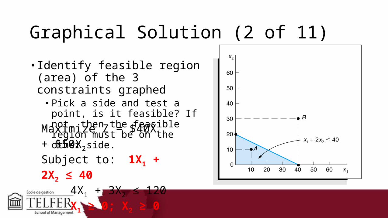
• Identify feasible region (area) of the 3 constraints graphed

• Pick a side and test a point, is it feasible? If not, then the feasible region must be on the other side.

Maximize Z = $40X1 + $50X2

Subject to: 1X1 + 2X2 ≤ 404X1 + 3X2 ≤ 120X1 ≥ 0; X2 ≥ 0

Graphical Solution (3 of 11)

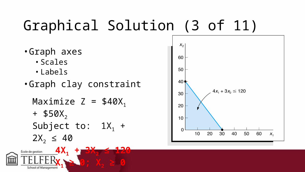
• Graph axes• Scales• Labels

• Graph clay constraint

Maximize Z = $40X1 + $50X2

Subject to: 1X1 + 2X2 ≤ 404X1 + 3X2 ≤ 120X1 ≥ 0; X2 ≥ 0

Graphical Solution (4 of 11)

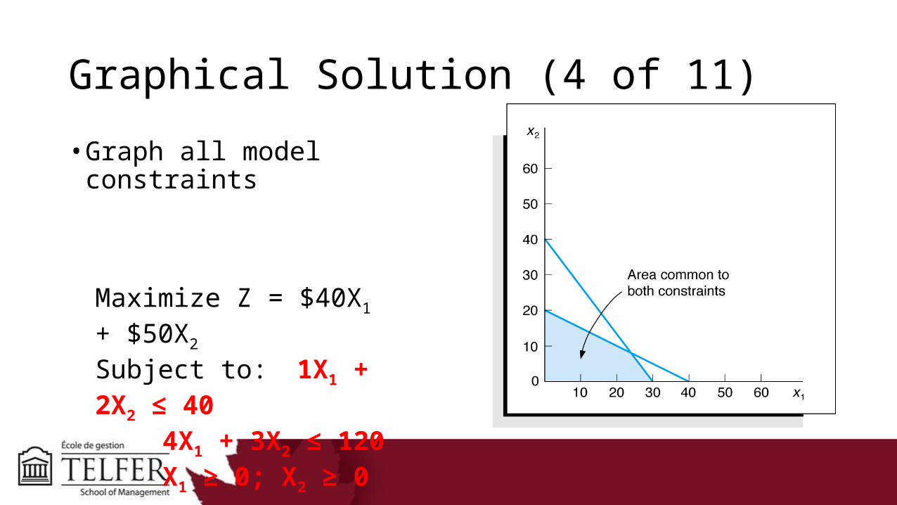
• Graph all model constraints

Maximize Z = $40X1 + $50X2

Subject to: 1X1 + 2X2 ≤ 404X1 + 3X2 ≤ 120X1 ≥ 0; X2 ≥ 0

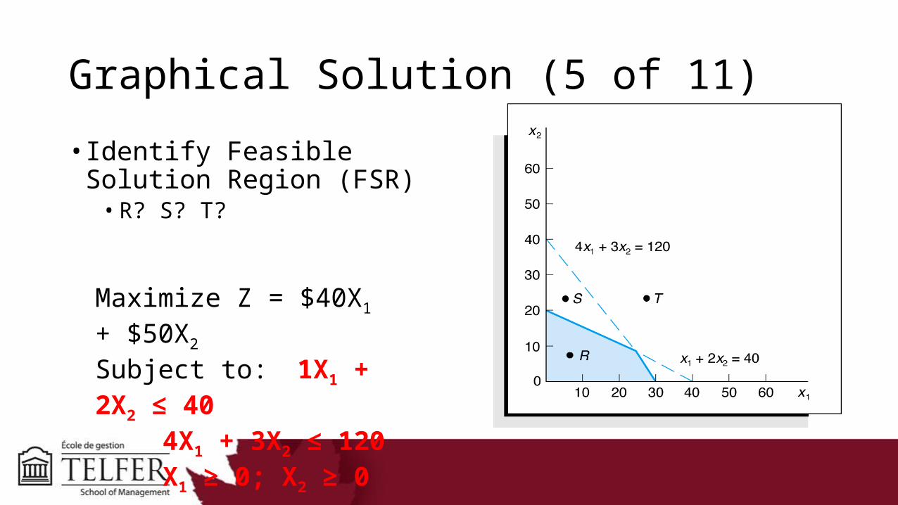
Graphical Solution (5 of 11)

• Identify Feasible Solution Region (FSR)

• R? S? T?

Maximize Z = $40X1 + $50X2

Subject to: 1X1 + 2X2 ≤ 404X1 + 3X2 ≤ 120X1 ≥ 0; X2 ≥ 0

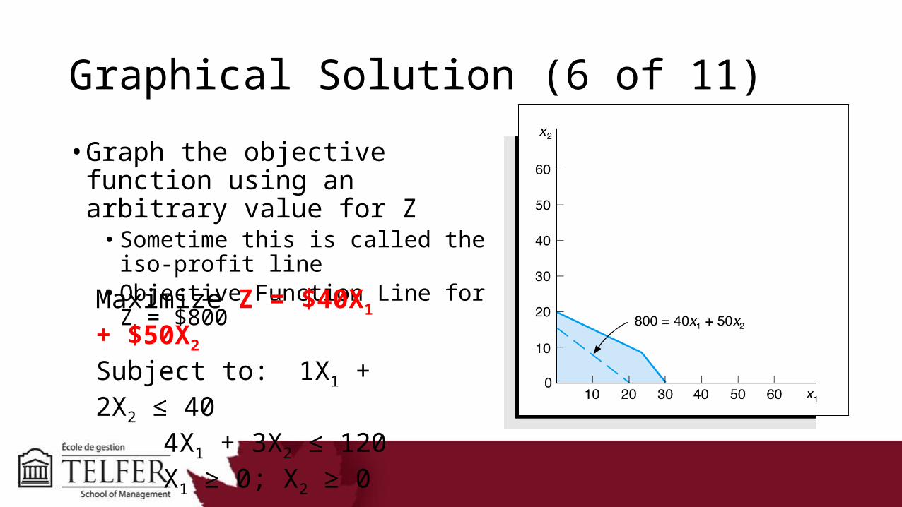
Graphical Solution (6 of 11)

• Graph the objective function using an arbitrary value for Z

• Sometime this is called the iso-profit line• Objective Function Line for Z = $800

Maximize Z = $40X1 + $50X2

Subject to: 1X1 + 2X2 ≤ 404X1 + 3X2 ≤ 120X1 ≥ 0; X2 ≥ 0

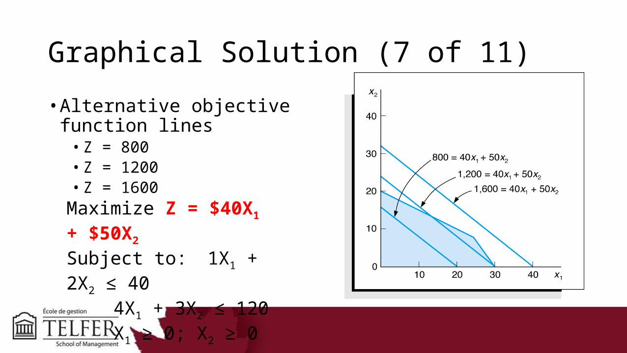
Graphical Solution (7 of 11)

• Alternative objective function lines• Z = 800• Z = 1200• Z = 1600

Maximize Z = $40X1 + $50X2

Subject to: 1X1 + 2X2 ≤ 404X1 + 3X2 ≤ 120X1 ≥ 0; X2 ≥ 0

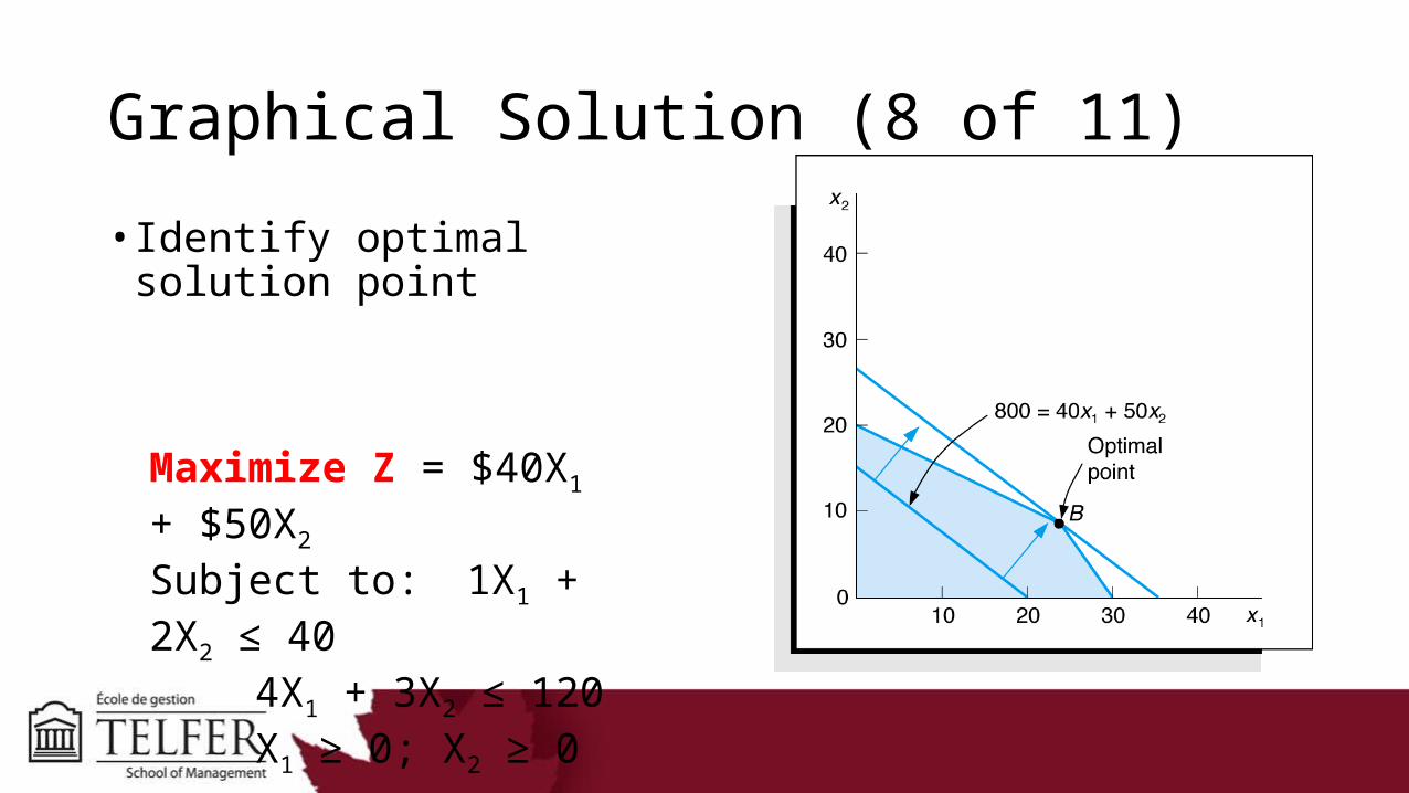
Graphical Solution (8 of 11)

• Identify optimal solution point

Maximize Z = $40X1 + $50X2

Subject to: 1X1 + 2X2 ≤ 404X1 + 3X2 ≤ 120X1 ≥ 0; X2 ≥ 0

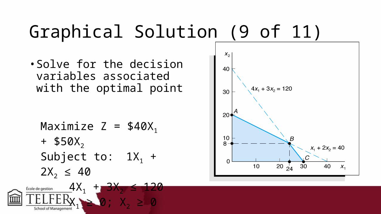
Graphical Solution (9 of 11)

• Solve for the decision variables associated with the optimal point

Maximize Z = $40X1 + $50X2

Subject to: 1X1 + 2X2 ≤ 404X1 + 3X2 ≤ 120X1 ≥ 0; X2 ≥ 0

Observation: Where would the optimal solutions always be?

• An optimal solution, if it exists, will always be at the corner of the feasible solution region (area).

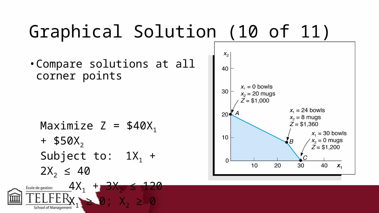
Graphical Solution (10 of 11)

• Compare solutions at all corner points

Maximize Z = $40X1 + $50X2

Subject to: 1X1 + 2X2 ≤ 404X1 + 3X2 ≤ 120X1 ≥ 0; X2 ≥ 0

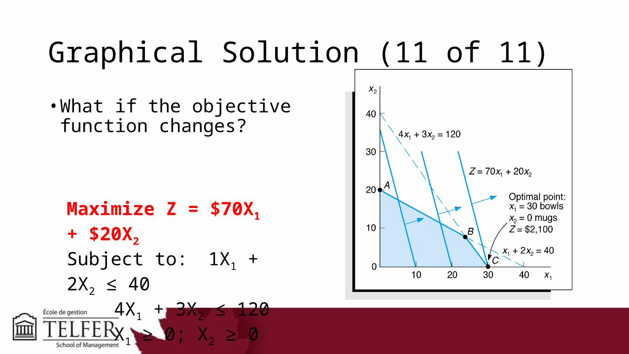
Graphical Solution (11 of 11)

• What if the objective function changes?

Maximize Z = $70X1 + $20X2

Subject to: 1X1 + 2X2 ≤ 404X1 + 3X2 ≤ 120X1 ≥ 0; X2 ≥ 0

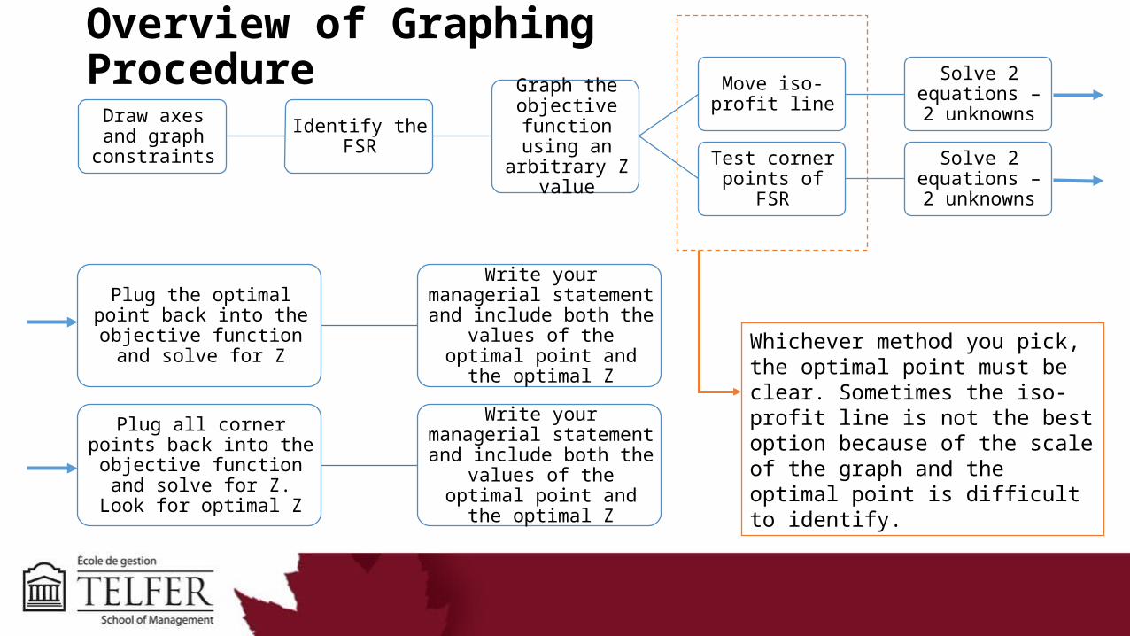
Overview of Graphing Procedure

Draw axes and graph constraints Identify the FSR

Graph the objective function using an arbitrary

Z value

Move iso-profit line

Solve 2 equations – 2 unknowns

Test corner points of FSR

Solve 2 equations – 2 unknowns

Plug the optimal point back into the objective function

and solve for Z

Write your managerial statement and include both

the values of the optimal point and the optimal Z

Plug all corner points back into the objective function

and solve for Z. Look for optimal Z

Write your managerial statement and include both

the values of the optimal point and the optimal Z

Whichever method you pick, the optimal point must be clear. Sometimes the iso-profit line is not the best option because of the scale of the graph and the optimal point is difficult to identify.

LP Model Formulation - Minimization Problem• Many LP problems involve minimizing objective such as cost instead

of maximizing profit function.

Examples:• Restaurant may wish to develop work schedule to meet staffing needs

while minimizing total number of employees. • Hospital may want to provide its patients with a daily meal plan that

meets certain nutritional standards while minimizing food purchase costs.

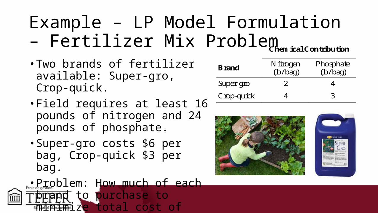
Example – LP Model Formulation – Fertilizer Mix Problem• Two brands of fertilizer available:

Super-gro, Crop-quick.• Field requires at least 16 pounds of

nitrogen and 24 pounds of phosphate.• Super-gro costs $6 per bag, Crop-quick

$3 per bag.• Problem: How much of each brand to

purchase to minimize total cost of fertilizer given following data?

Chemical Contribution

Brand Nitrogen (lb/ bag)

Phosphate (lb/ bag)

Super-gro 2 4

Crop-quick 4 3

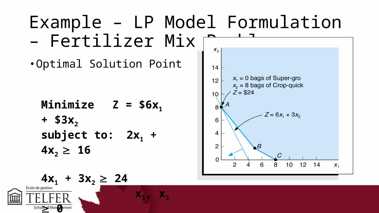
Example – LP Model Formulation – Fertilizer Mix Problem• Optimal Solution Point

Minimize Z = $6x1 + $3x2

subject to: 2x1 + 4x2 16 4x1 + 3x2 24

x1, x2 0

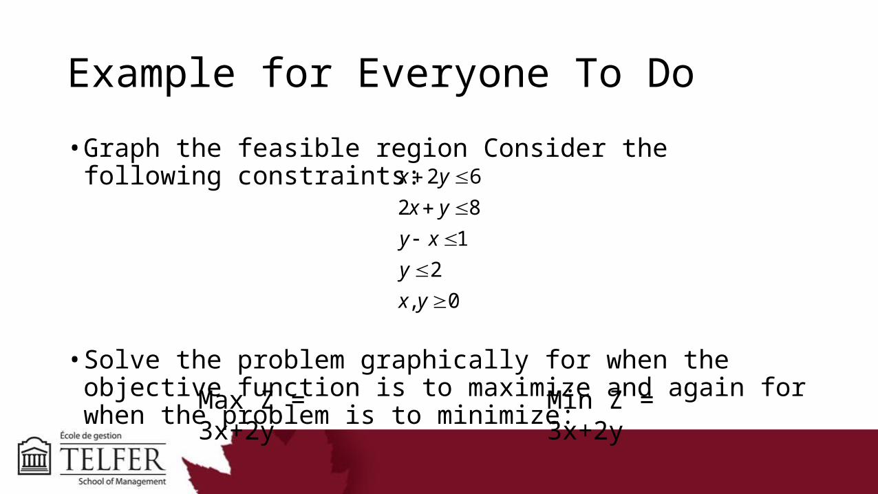
Example for Everyone To Do

• Graph the feasible region Consider the following constraints:

• Solve the problem graphically for when the objective function is to maximize and again for when the problem is to minimize:

2 6

2 8

1

2

, 0

x y

x y

y x

y

x y

Max Z = 3x+2y Min Z = 3x+2y

If this was a maximization problem, we move the objective function away from the origin. Therefore the optimal solution is found at point E

If this was a minimization problem, we move the objective function towards the origin. Therefore the optimal solution is found at point A

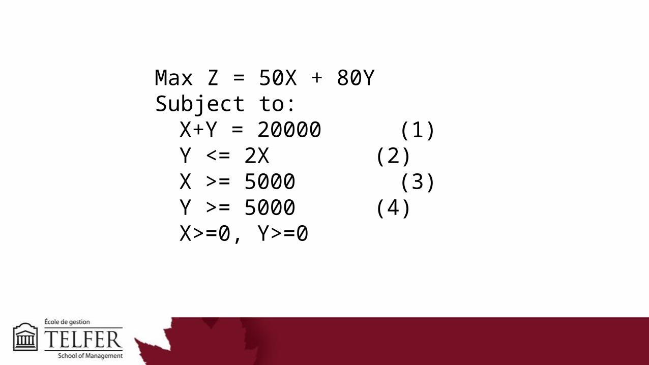
Max Z = 50X + 80YSubject to:

X+Y = 20000 (1)Y <= 2X (2)X >= 5000 (3)Y >= 5000 (4)X>=0, Y>=0

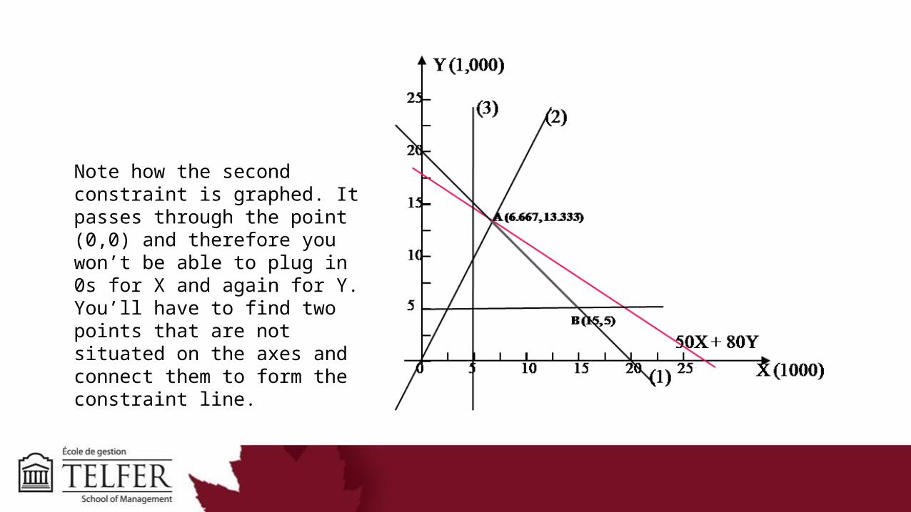
Note how the second constraint is graphed. It passes through the point (0,0) and therefore you won’t be able to plug in 0s for X and again for Y. You’ll have to find two points that are not situated on the axes and connect them to form the constraint line.

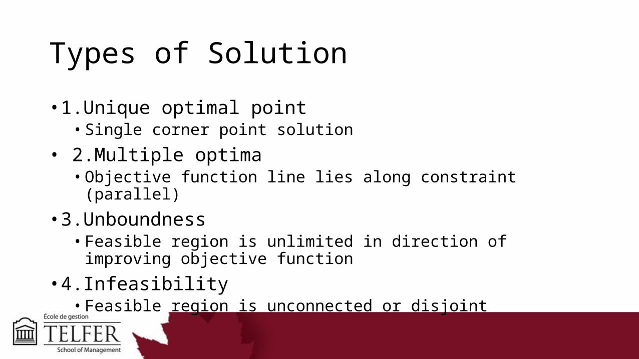
Types of Solution

• 1.Unique optimal point• Single corner point solution

• 2.Multiple optima• Objective function line lies along constraint (parallel)

• 3.Unboundness• Feasible region is unlimited in direction of improving objective function

• 4.Infeasibility• Feasible region is unconnected or disjoint

Special Cases of LP Models

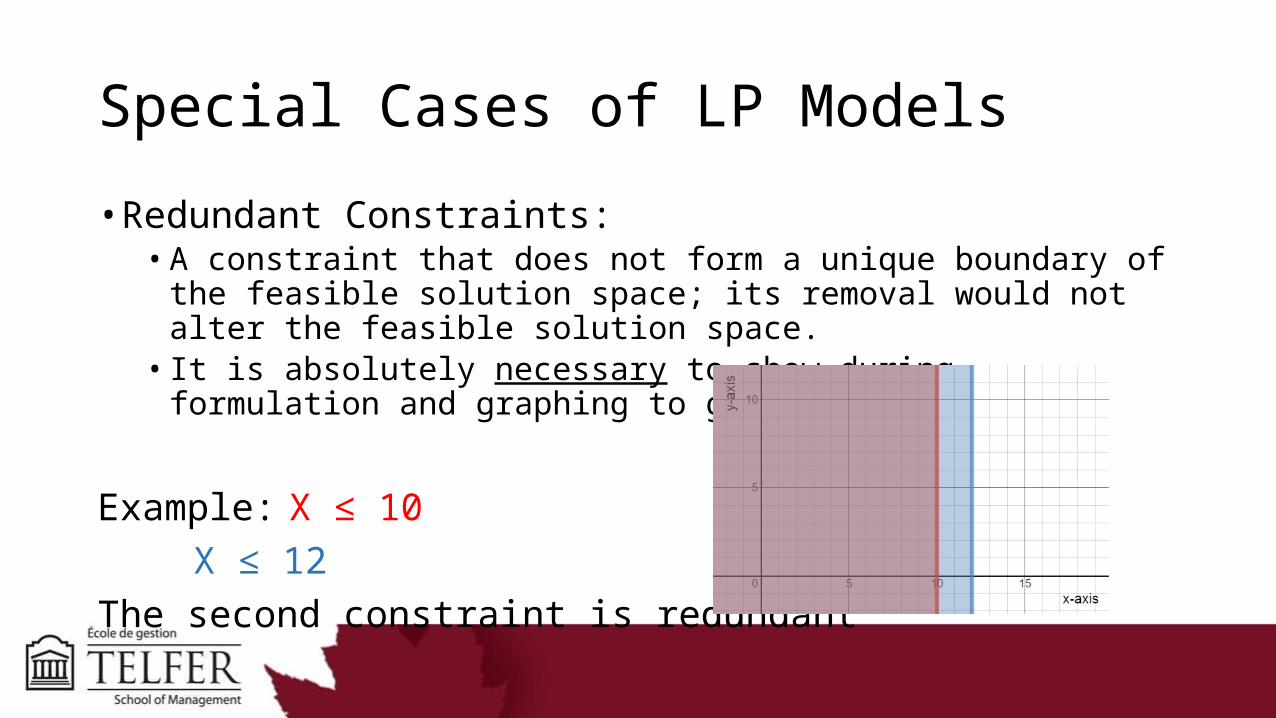
• Redundant Constraints:• A constraint that does not form a unique boundary of the feasible solution

space; its removal would not alter the feasible solution space.• It is absolutely necessary to show during formulation and graphing to get full

marks.

Example: X ≤ 10X ≤ 12

The second constraint is redundant

Special Cases of LP Models

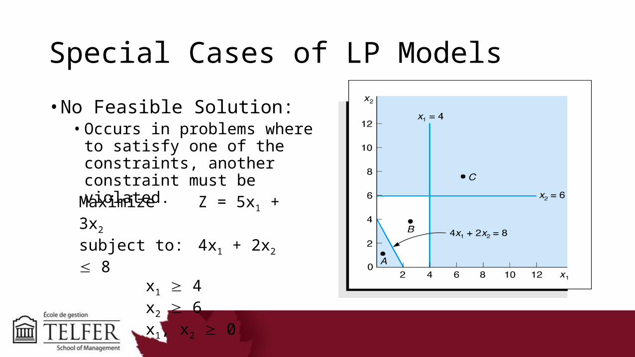
• No Feasible Solution:• Occurs in problems where to satisfy

one of the constraints, another constraint must be violated.

Maximize Z = 5x1 + 3x2

subject to: 4x1 + 2x2 8 x1 4 x2 6 x1, x2 0

Special Cases of LP Models

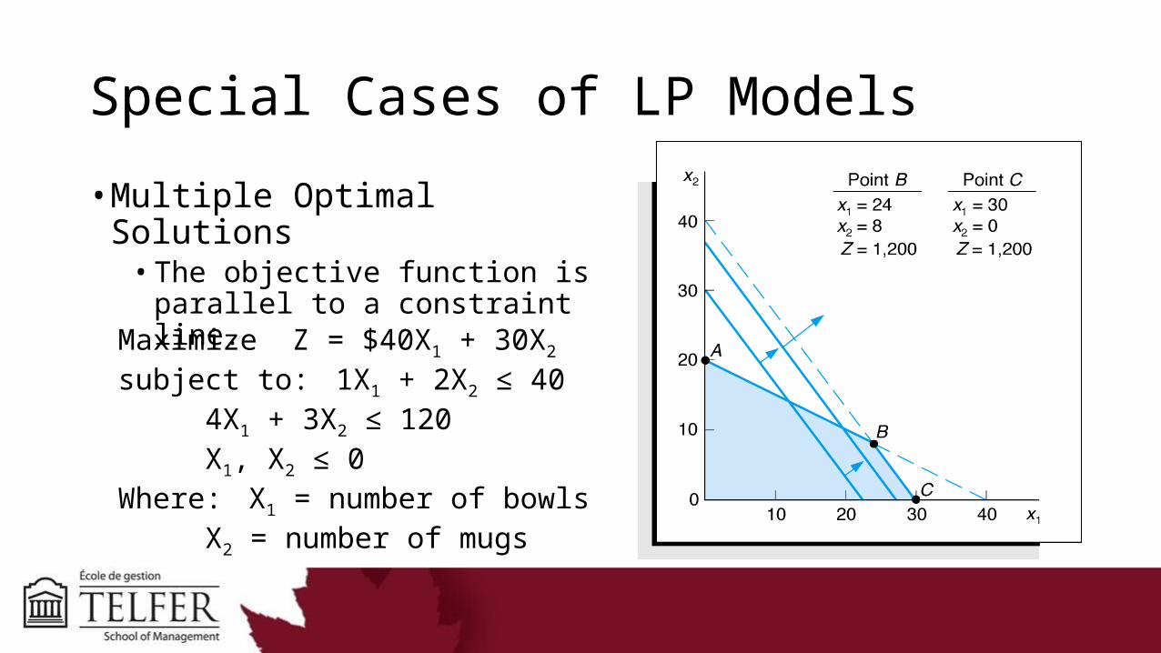
• Multiple Optimal Solutions• The objective function is parallel to a

constraint line.

Maximize Z = $40X1 + 30X2

subject to: 1X1 + 2X2 ≤ 404X1 + 3X2 ≤ 120X1, X2 ≤ 0

Where: X1 = number of bowlsX2 = number of mugs

Special Cases of LP Models

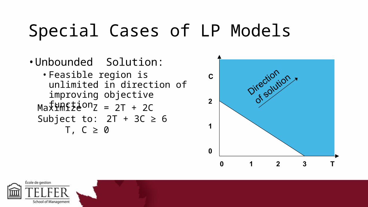
• Unbounded Solution:• Feasible region is unlimited in direction

of improving objective function

Maximize Z = 2T + 2CSubject to: 2T + 3C ≥ 6

T, C ≥ 0

Online Graphing Tool

An online graphing tool for you to use to check your graph and get a sense of the feasible solution region. However, you need to be able to solve by hand without any online tools for the midterm and final exam. Any graphs on the assignment are to be done by hand as well. No marks will be awarded if you submit a computer generated graph.

https://www.desmos.com/calculator