Administrative TasksTurn in your HWSample Research

PaperBuckle your

seatbelts we have a lot to cover

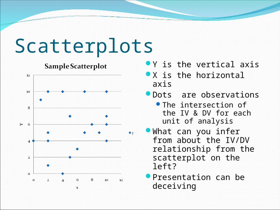
ScatterplotsY is the vertical axisX is the horizontal axisDots are observations

The intersection of the IV & DV for each unit of analysis

What can you infer from about the IV/DV relationship from the scatterplot on the left?

Presentation can be deceiving

Three factors to consider when analyzing scatterplotsDirectionality

Do the dots appear to flow in a particular direction?Or, does the scatterplot look more like white noise (like a

TV when it doesn’t have a signal)?The more it looks like white noise the less the two

variables are relatedClustering

Are the majority of the dots in a small area of the graph?How would this impact our confidence in predictions

outside of this area?Outliers

Are there cases that differ markedly from the overall pattern of the dots? i.e. not near the cluster or contrary to the directionality

Which observations are these? How influential are these cases?

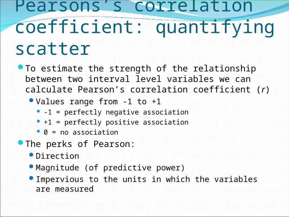
Pearsons’s correlation coefficient: quantifying scatterTo estimate the strength of the relationship

between two interval level variables we can calculate Pearson’s correlation coefficient (r)Values range from -1 to +1

-1 = perfectly negative association +1 = perfectly positive association 0 = no association

The perks of Pearson:DirectionMagnitude (of predictive power)Impervious to the units in which the variables are

measured

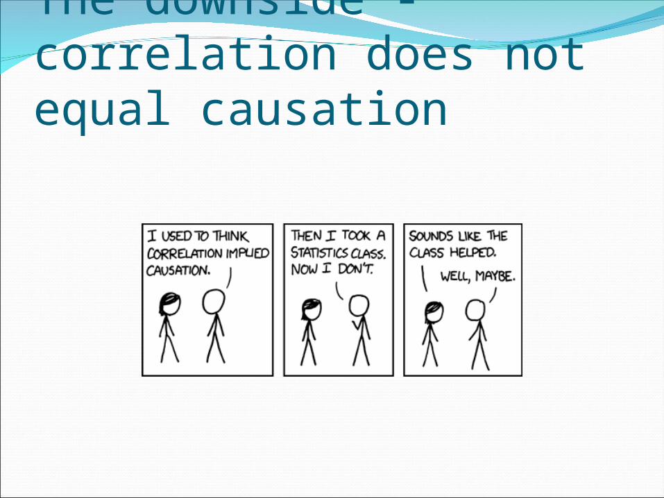
The downside - correlation does not equal causation

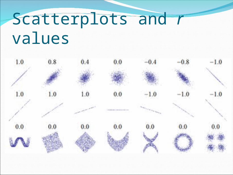
Scatterplots and r values

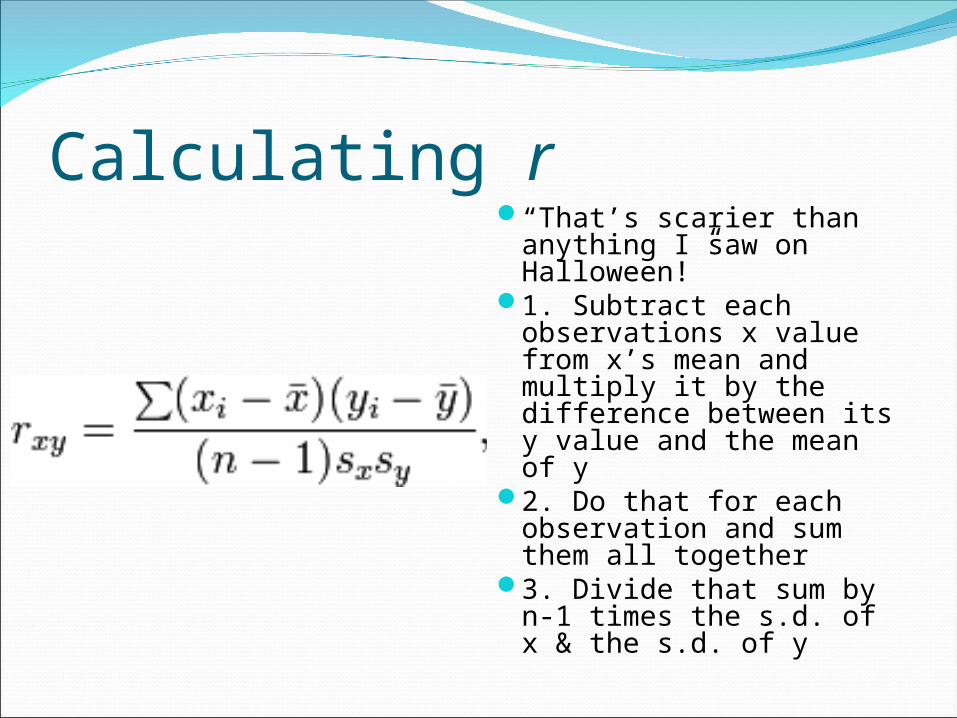
Calculating r“That’s scarier than

anything I saw on Halloween!”

1. Subtract each observations x value from x’s mean and multiply it by the difference between its y value and the mean of y

2. Do that for each observation and sum them all together

3. Divide that sum by n-1 times the s.d. of x & the s.d. of y

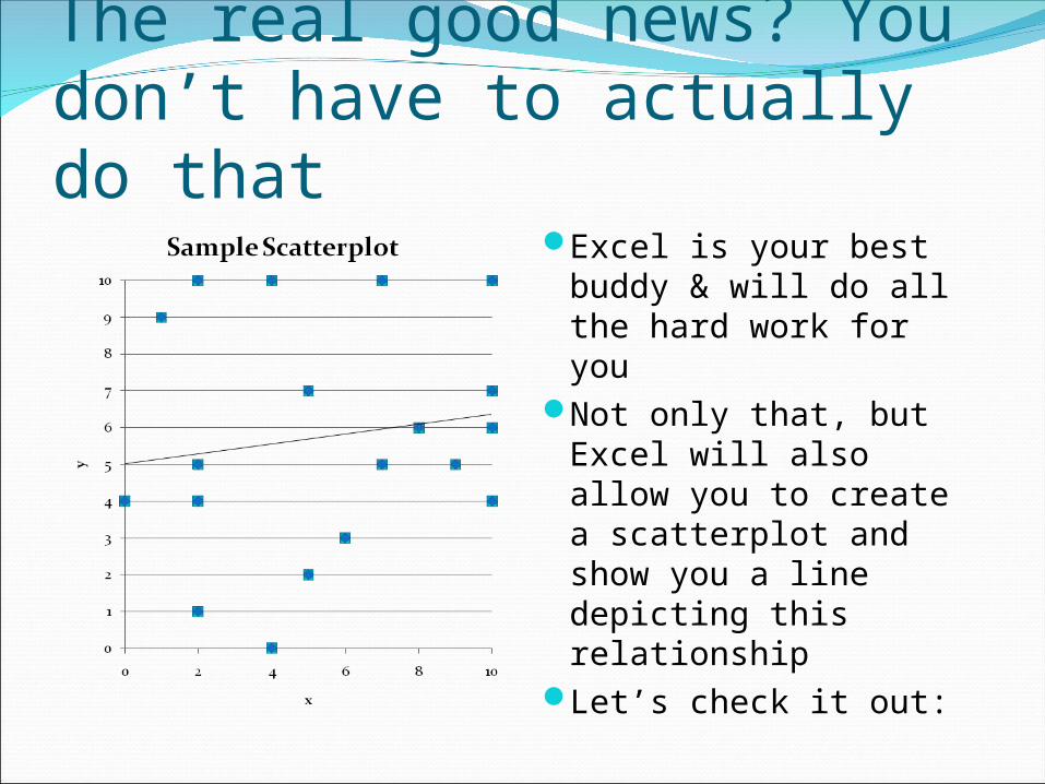
The real good news? You don’t have to actually do that

Excel is your best buddy & will do all the hard work for you

Not only that, but Excel will also allow you to create a scatterplot and show you a line depicting this relationship

Let’s check it out:

“Tell me more about this line!”Slope:

Change in Y divided by change in X

InterceptValue of Y when X = O

ErrorDistance between the

line’s Y value and a data point’s Y value

The line minimizes the sum of all the squared errors

“I love line!”

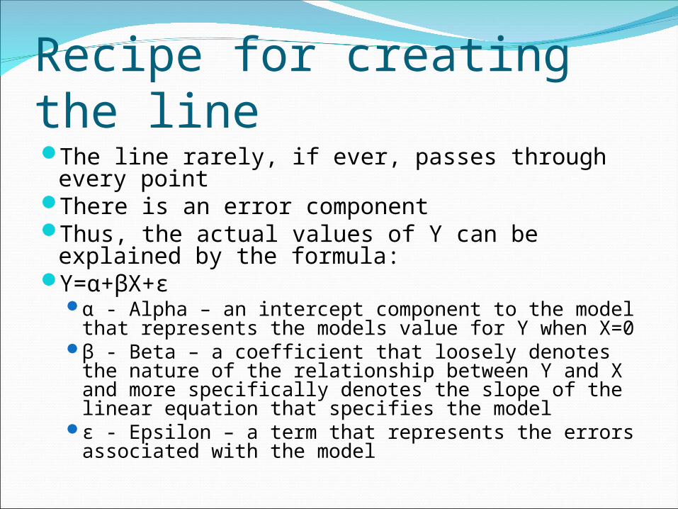
Recipe for creating the lineThe line rarely, if ever, passes through

every pointThere is an error componentThus, the actual values of Y can be

explained by the formula:Y=α+βX+ε

α - Alpha – an intercept component to the model that represents the models value for Y when X=0

β - Beta – a coefficient that loosely denotes the nature of the relationship between Y and X and more specifically denotes the slope of the linear equation that specifies the model

ε - Epsilon – a term that represents the errors associated with the model

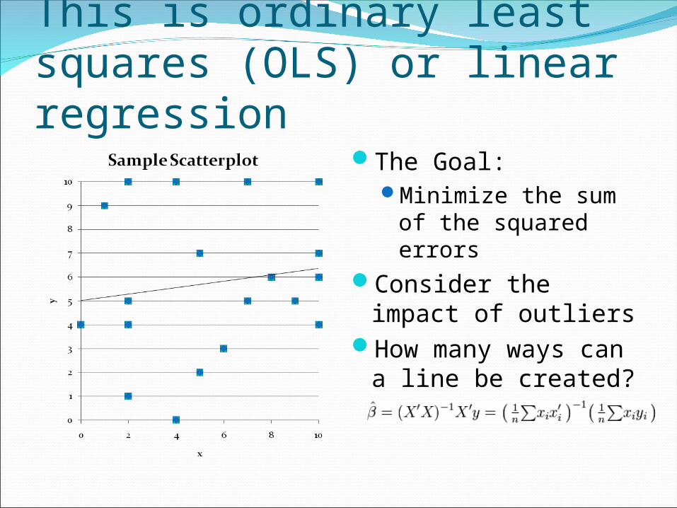
This is ordinary least squares (OLS) or linear regression

The Goal:Minimize the sum of

the squared errorsConsider the impact

of outliersHow many ways can

a line be created?

“Not gonna do it. Wouldn’t be prudent.”

You know the trick:It’s not as hard as it looks

You are really comparing Y’s deviations from it’s mean alongside X’s deviation from it’s meanSee the formula at the

bottom of pg. 331Ideally the Xi’s move in

sync with the Yi’s divergence from the meanThis is covariation

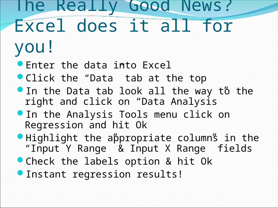
The Really Good News? Excel does it all for you!Enter the data into ExcelClick the “Data” tab at the topIn the Data tab look all the way to the right

and click on “Data Analysis”In the Analysis Tools menu click on

Regression and hit OkHighlight the appropriate columns in the

“Input Y Range” & Input X Range” fieldsCheck the labels option & hit OkInstant regression results!

What to look for when examining regression outputBeta coefficient:

DirectionalitySize of the coefficientStandard ErrorStatistical Significance

ConstantFar less important than

BetaWhen X = O what

would we expect Y to be? Is X ever O?

Goodness of fitHow much of the

variation in Y is actually explained by X?

How “good” does your model “fit” the actual values of Y?

R-squared (the coefficient of determination) provides an estimate

r Strikes Back!Recall that r, Pearson’s

correlation coefficient, measures the degree to which two variables co-vary

With OLS the:Constant tells us where

the line startsBeta tells us how the line

slopesR-squared tells us the %

of the variation in Y our model predicts Range 0-1

O = Predicts none of the variation

1 = Predicts all of the variation