Embed Size (px)
Citation preview

8
Correlation and simple linear regression
Correlation and regression are techniques used to examine associations and rela-
tionships between continuous variables collected on the same set of sampling or
experimental units. Specifically, correlation is used to investigate the degree to which
variables change or vary together (covary). In correlation, there is no distinction
between dependent (response) and independent (predictor) variables and there is no
attempt to prescribe or interpret the causality of the association. For example, there
may be an association between arm and leg length in humans, whereby individu-
als with longer arms generally have longer legs. Neither variable directly causes the
change in the other. Rather, they are both influenced by other variables to which
they both have similar responses. Hence correlations apply mainly to survey designs
where each variable is measured rather than specifically set or manipulated by the
investigator.
Regression is used to investigate the nature of a relationship between variables
in which the magnitude and changes in one variable (known as the independent or
predictor variable) are assumed tobedirectly responsible for themagnitude andchanges
in the other variable (dependent or response variable). Regression analyses apply to
both survey and experimental designs. Whilst for experimental designs, the direction
of causality is established and dictated by the experiment, for surveys the direction of
causality is somewhat discretionary and based on prior knowledge. For example,
although it is possible that ambient temperature effects the growth rate of a species of
plant, the reverse is not logical. As an example of regression, we could experimentally
investigate the relationship between algal cover on rocks and molluscan grazer density
by directly manipulating the density of snails in different specifically control plots and
measuring the cover of algae therein. Any established relationship must be driven by
snail density, as this was the controlled variable. Alternatively the relationship could be
investigated via a field survey in which the density of snails and cover of algae could
be measured from random locations across a rock platform. In this case, the direction
of causality (or indeed the assumption of causality) may be more difficult to defend.
In addition to examining the strength and significance of a relationship (for
which correlation and regression are equivalent), regression analysis also explores the
functional nature of the relationship. In particular, it estimates the rate at which a
change in an independent variable is reflected in a change in a dependent variable as
Biostatistical Design and Analysis Using R: a Practical Guide, 1st edition. By M. Logan.Published 2010 by Blackwell Publishing.
168 CHAPTER 8
well as the expected value of the dependent variable when the independent variable is
equal to zero. These estimates can be used to construct a predictive model (equation)
that relates the magnitude of a dependent variable to the magnitude of an independent
variable, and thus permit new responses to be predicted from new values of the
independent variable.
8.1 Correlation
The simplest measure of association between two variables is the sum product of the
deviations of each point from the mean center [e.g.�
(x − x)(y − y)], see Figure. 8.1f.
Thismethod essentially partitions the cloudof points up into four quadrants andweighs
up the amount in the positive and negative quadrants. The greater the degree to which
points are unevenly distributed across the positive and negative quadrants, the greater
the magnitude (either negative or positive) of the measure of association. Clearly how-
ever, the greater thenumber of points, thehigher themeasure of association.Covariance
standardizes for sample size by dividing this measure by the degrees of freedom (num-
ber of observation pairs minus 1) and thus represents the average deviations from the
mean center. Note that covariance is really the bivariate variance of two variablesa.
2 8 10
X units
2
4
6
8
10
Y u
nits
(a)
cov = 3.5cor = 0.7
20 40 60 80 100
X units
2
4
6
8
10
Y u
nits
(b)
cov = 35cor = 0.7
2 8 10
X units
2
4
6
8
10Y
un
its
(c)
cov = −3.5cor = −0.7
X units
2
4
6
8
10
Y u
nits
(d)
cov = 4.75cor = 0.95
X units
2
4
6
8
10
Y u
nits
(e)
cov = 0 cor = 0
X
Y
xi − x (−ve)
yi
− y
(−
ve)
−ve deviation
−ve deviation+ve deviation
+ve deviation
(f)
4 64 6
2 8 104 6 2 8 104 6
Fig 8.1 Fictitious data illustrating covariance, correlation, strength and polarity.
a Covariance of a single variable and itself is the variance of that variable.

CORRELATION AND SIMPLE LINEAR REGRESSION 169
8.1.1 Product moment correlation coefficient
Unfortunately, there are no limits on the range of covariance as its magnitude
depends on the scale of the units of the variables (see Figure 8.1a-b). The Pearson’s
(product moment) correlation coefficient further standardizes covariance by dividing
it by the standard deviations of x and y, thereby resulting in a standard coefficient
(ranging from −1 to +1) that represents the strength and polarity of a linear
association.
8.1.2 Null hypothesis
Correlation tests the H0 that the population correlation coefficient (ρ, estimated by
the sample correlation coefficient, r) equals zero:
H0 : ρ = 0 (the population correlation coefficient equals zero)
This null hypothesis is tested using a t statistic (t = rsr), where sr is the standard error
of r. This t statistic is compared to a t distribution with n− 2 degrees of freedom.
8.1.3 Assumptions
In order that the calculated t-statistic should reliably represent the population trends,
the following assumptions must be met:
(i) linearity - as the Pearson correlation coefficient measures the strength of a linear (straight-
line) association, it is important to establish whether or not some other curved relationship
represents the trends better. Scatterplots are useful for exploring linearity.
(ii) normality - the calculated t statistic will only reliably follow the theoretical t distribution
when the joint XY population distribution is bivariate normal. This situation is only
satisfied when both individual populations (X and Y) are themselves normally distributed.
Boxplots should be used to explore normality of each variable.
Scale transformations are often useful to improve linearity and non-normality.
8.1.4 Robust correlation
For situations when one or both of the above assumptions are not met and transfor-
mations are either unsuccessful or not appropriate (particularly, proportions, indices
and counts), monotonic associations (general positive or negative - not polynomial)
can be investigated using non-parametric (rank-based) tests. The Spearman’s rank
correlation coefficient (rs) calculates the product moment correlation coefficient on
the ranks of the x and y variables and is suitable for samples with between 7 and 30
observations. For greater sample sizes, an alternative rank based coefficient Kendall’s
(τ ) is more suitable. Note that non-parametric tests are more conservative (have less
power) than parametric tests.
170 CHAPTER 8
8.1.5 Confidence ellipses
Confidence ellipses are used to represent the region on a plot within which we have
a certain degree of confidence (e.g 95%) the true population mean center is likely to
occur. Such ellipses are centered at the sample mean center and oriented according to
the covariance matrixb of x and y.
8.2 Simple linear regression
Simple linear regression is concernedwith generating amathematical equation (model)
that relates the magnitude of dependent (response) variable to the magnitude of the
independent (predictor) variable. The general equation for a straight line is y = bx + a,
where a is the y-intercept (value of y when x = 0) and b is the gradient or slope (rate
at which y changes per unit change in x).
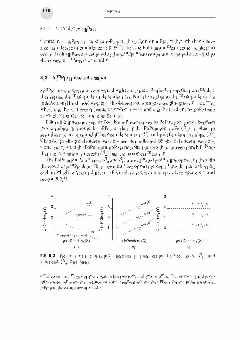
Figure 8.2 illustrates sets of possible representatives of population trends between
two variables. It should be apparent that if the population slope (β1) is equal to
zero there is no relationship between dependent (Y) and independent variables (X).
Changes in the independent variable are not reflected by the dependent variable.
Conversely, when the population slope is not equal to zero there is a relationship. Note
that the population intercept (β0) has less biological meaning.
The population parameters (β0 and β1) are estimated from a line of best fit through
the cloud of sample data. There are a number of ways to determine the line of best fit,
each of which represent different approach to regression analysis (see Figure 8.4, and
section 8.2.5).
Independent (X)
1
2
3
4
Dependent (Y
)
(a)
Slope (b1) = 0
b1 <0
Independent (X)
1
2
3
4
Dependent (Y
)
(b)
b 0= 2, b 1
>0
b 0= 1, b 1
>0
b 0= 0, b 1
>0
Independent (X)
0
1
2
3
Dependent (Y
)
(c)
b0= 2, b
1= 0
b0= 1, b
1= 0
b0= 0, b
1= 0
Y-intercept(b0) = 2 for all
b 1>0
Fig 8.2 Fictitious data contrasting differences in interpretation between slope (β1) and
y-intercept (β0) parameters.
b The covariance matrix of two variables has two rows and two columns. The upper left and lower
right entries represent the variances of x and y respectively and the upper right and lower left entries
represent the covariance of x and y.
CORRELATION AND SIMPLE LINEAR REGRESSION 171
8.2.1 Linear model
The linear model reflects the equation of the line of best fit:
yi = β0 + β1xi + εi
where β0 is the population y-intercept, β1 is the population slope and εi is the random
unexplained error or residual component.
8.2.2 Null hypotheses
A separate H0 is tested for each of the estimated model parameters:
H0 : β1 = 0 (the population slope equals zero)
This test examines whether or not there is likely to be a relationship between the
dependent and independent variables in the population. In simple linear regression, this
test is identical to the test that thepopulation correlation coefficient equals zero (ρ = 0).
H0 : β0 = 0 (the population y-intercept equals zero)
This test is rarely of interest as it only tests the likelihood that the background level
of the response variable is equal to zero (rarely a biologically meaningful comparison)
and does not test whether or not there is a relationship (see Figure 8.4b-c).
These H0’s are tested using a t statistic (e.g. t = bsb
), where sb is the standard error
of b. This t statistic is compared to a t distribution with n− 2 degrees of freedom.
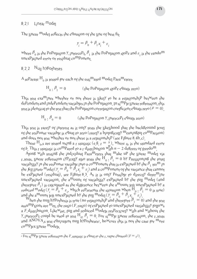
Along with testing the individual parameters that make up the linear model via
t-tests, linear regression typically also tests the H0 : β1 = 0 by partitioning the total
variability in the response variable into a component that is explained by the β1 term in
the full linear model (yi = β0 + β1xi + εi) and a component of the variance that cannot
be explained (residual), see Figure 8.3. As it is only possible to directly determine
unexplained variation, the amount of variability explained by the full model (and
therefore β1) is calculated as the difference between the amount left unexplained by a
reduced model (yi = β0 + εi, which represents the situation when H0 : β1 = 0 is true)
and the amount left unexplained by the full model (yi = β0 + β1xi + εi).
When the null hypothesis is true (no relationship and therefore β1 = 0) and the test
assumptions are met, the ratio (F-ratio) of explained to unexplained variability follows
a F-distribution. Likewise, full and reduced models respectively with and without the
y-intercept could be used to test H0: β1 = 0. For simple linear regression, the t-tests
and ANOVA’s test equivalent null hypothesesc, however this is not the case for more
complex linear models.
c For simple linear regression the F-statistic is equal to the t-value squared (F = t2).
172 CHAPTER 8
2 8 12
X units
2
4
6
8
10
12
14
16
Y u
nits
SStotal
= sum of squared total distances
MStotal
= response variance
=SS
total
dftotal
Overall mean
2
4
6
8
10
12
14
16
Y u
nits
SSregression
= sum of squared explained distances
MSregression
= conservative mean var explained
=SS
regression
dfregression
Overall mean
Predicted trend
Explained variabilty (distances)
X units
2
4
6
8
10
12
14
16
Y u
nits
(c)
SSresidual
= sum of squared unexplained distances
MSresidual
= conservative mean var unexplained
=SS
residual
dfresidual
Predicted trend
Explained variability (distances) F-ratio =
Explained
Unexplained=
MSgroups
MSresidual
F-distribution(Distribution of all possible expected F-ratios when the H
0 is true)
(d)
(a) (b)
104 6 2 8 12
X units
104 6
2 8 12104 6 0 1 2 3 4 5
Fig 8.3 Fictitious data illustrating the partitioning of (a) total variation into components
(b) explained (MSregression) and (c) unexplained (MSresidual) by the linear trend. The probability of
collecting our sample, and thus generating the sample ratio of explained to unexplained variation
(or one more extreme), when the null hypothesis is true (and there is no relationship between
X and Y) is the area under the F-distribution (d) beyond the sample F-ratio.
8.2.3 Assumptions
To maximize the reliability of null hypotheses tests, the following assumptions
apply:
(i) linearity - simple linear regression models a linear (straight-line) relationship and thus it
is important to establish whether or not some other curved relationship represents the
trends better. Scatterplots are useful for exploring linearity.
(ii) normality - the populations from which the single responses were collected per level of
the predictor variable are assumed to be normally distributed. Boxplots of the response
variable (and predictor if it was measured rather than set) should be used to explore
normality.

CORRELATION AND SIMPLE LINEAR REGRESSION 173
(iii) homogeneity of variance - the populations from which the single responses were
collected per level of the predictor variable are assumed to be equally varied. With only
a single representative of each population per level of the predictor variable, this can
only be explored by examining the spread of responses around the fitted regression line.
In particular, increasing spread along the regression line would suggest a relationship
between population mean and variance (which must be independent to ensure unbiased
parameter estimates). This can also be diagnosed with a residual plot.
8.2.4 Multiple responses for each level of the predictor
Simple linear regression assumes linearity and investigates whether there is a relation-
ship between a response and predictor variable. In so doing, it is relying on single
response values at each level of the predictor being good representatives of their
respective populations. Having multiple independent replicates of each population
from which a mean can be calculated thereby provides better data from which to
investigate a relationship. Furthermore, the presence of replicates of the populations at
each level of the predictor variable enables us to establish whether or not the observed
responses differ significantly from their predicted values along a linear regression line
and thus to investigate whether the population relationship is linear versus some other
curvilinear relationship. Analysis of such data is equivalent to ANOVAwith polynomial
contrasts (see section 10.6).
8.2.5 Model I and II regression
The ordinary least squares (OLS, or model I regression) fits a line that minimizes
the vertical spread of values around the line and is the standard regression procedure.
Regression was originally devised to explore the nature of relationship between a
measured dependent variable and an independent variable of which the levels where
specifically set (and thus controlled) by the researcher to represent a uniform range of
possibilities. As the independent variable is set (fixed) rather than measured, there is no
uncertainty or error in the y values. The coordinates predicted (by the linear model) for
any given observation must therefore lie in a vertical plane around the observed coordi-
nates (see Figure 8.4a). The difference between anobserved value and its predicted value
is called a residual. Hence, OLS regression minimizes the sum of the squaredd residuals.
Model II regression refers to a family of line fitting procedures that acknowledge
and incorporate uncertainty in both response and predictor variables and primarily
describe the first major axis through a bivariate normal distribution (see Table 8.1 and
Figure 8.4). These techniques generate better parameter estimates (such as population
slope) than model I regression when the levels of the predictor variable are measured,
however, they are only necessary for situations in which the parameter estimates are
the main interest of the analysis. For example, when performing regression analysis
d Residuals are squared to remove negatives. Since the regression line is fitted exactly through the
middle of the cloud of points, some points will be above this line (+ve residuals) and some points
will be below (-ve residuals) and therefore the sum of the residuals will equal exactly zero.
174 CHAPTER 8
20 40 60 80 100
X units
2
4
6
8
10
Y u
nits
(a) OLS Y against X
20 40 60 80 100
X units
2
4
6
8
10
Y u
nits
(d) ranged MA
20 40 60 80 100
X units
2
4
6
8
10
Y u
nits
(b) OLS X against Y
20 40 60 80 100
X units
2
4
6
8
10Y
un
its
(c) RMA
108642
X units
2
4
6
8
10
Y u
nits
(c) MA
(d)
20 40 60 80 100
X units
2
4
6
8
10
Y u
nits
OLS Y vs X&MA
OLS X vs Y
RMA
ranged MA
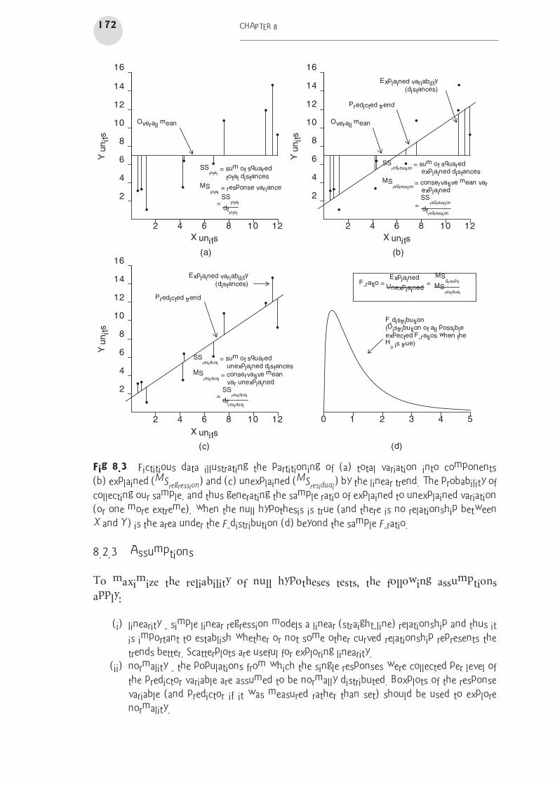
Fig 8.4 Fictitious data illustrating the differences between (a) ordinary least squares, (b) major
axis and (c) reduced major axis regression. Each are also contrasted in (d) along with a depiction
of ordinary least squares regression for X against Y. Note that the fitted line for all techniques
passes through the center mean of the data cloud. When the X and Y are measured on the same
scale, MA and RMA are the same.
to estimate the slope in allometric scaling relationships or to compare slopes between
models.
Major axis (MA) minimizes the sum square of the perpendicular spread from the
regression line (Figure 8.4c) and thus the predicted values line in a perpendicular
planes from the regression line. Although this technique incorporates uncertainty in
both response and predictor variable, it assumes that the degree of uncertainty is the
same on both axes (1:1 ratio) and is therefore only appropriate when both variables
are measured on the same scale and with the same units. Ranged major axis (Ranged
MA) is a modification of major axis regression in which MA regression is performed
on variables that are pre-standardized by their ranges (Figure 8.4d) and the resulting
parameters are then returned to their original scales. Alternatively,Reducedmajor axis
(RMA)minimizes the sum squared triangular areas bounded by the observations and
the regression line (Figure 8.4e) thereby incorporating all possible ratios of uncertainty
between the response and predictor variables. For this technique, the estimated slope
is the average of the slope from a regression of y against x and the inverse of the slope
of x against y.

CORRELATION AND SIMPLE LINEAR REGRESSION 175
Table 8.1 Comparison of the situations in which the different regression methods are suitable.
Method
Ordinary least squares (OLS)
• When there is no uncertainty in IV (levels set not measured) or uncertainty in IV �
uncertainty in DV
• When testing H0 : β1 = 0 (no linear relationship between DV and IV)
• When generating predictive models from which new values of DV are predicted from given
values of IV . Since we rarely have estimates of uncertainty in our new predictor values (and
thus must assume there is no uncertainty), predictions likewise must be based on predictive
models developed with the assumption of no uncertainty. Note, if there is uncertainty in IV ,
standard errors and confidence intervals inappropriate.
• When distribution is not bivariate normal
> summary(lm(DV~IV, data))
Major axis (MA)
• When a good estimate of the population parameters (slope) is required AND
• When distribution is bivariate normal (IV levels not set) AND
• When error variance (uncertainty) in IV and DV equal (typically because variables in same
units or dimensionless)
> library(biology)
> summary(lm.II(DV~IV, data, method=’MA’))
Ranged Major axis (Ranged MA)
• When a good estimate of the population parameters (slope) is required AND
• When distribution is bivariate normal (IV levels not set) AND
• When error variances are proportional to variable variances AND
• There are no outliers
> library(biology)
> #For variables whose theoretical minimum is arbitrary
> summary(lm.II(DV~IV, data, method=’rMA’))
> #OR for variables whose theoretical minimum must be zero
> #such as ratios, scaled variables & abundances
> summary(lm.II(DV~IV, data, method=’rMA’, zero=T))
Reduced major axis (RMA) or Standard major axis (SMA)
• When a good estimate of the population parameters (slope) is required AND
• When distribution is bivariate normal (IV levels not set) AND
• When error variances are proportional to variable variances AND
• When there is a significant correlation r between IV and DV
> library(biology)
> summary(lm.II(DV~IV, data, method=’RMA’))
Modified from Legendre (2001).

176 CHAPTER 8
8.2.6 Regression diagnostics
As part of linear model fitting, a suite of diagnostic measures can be calculated each of
which provide an indication of the appropriateness of the model for the data and the
indication of each points influence (and outlyingness) of each point on resulting the
model.
Leverage
Leverage is a measure of how much of an outlier each point is in x-space (on x-axis)
and thus only applies to the predictor variable. Values greater than 2 ∗ p/n (where
p=number of model parameters (p = 2 for simple linear regression), and n is the
number of observations) should be investigated as potential outliers.
Residuals
As the residuals are the differences between the observed and predicted values along a
vertical plane, they provide ameasure of howmuch of an outlier each point is in y-space
(on y-axis). Outliers are identified by relatively large residual values. Residuals can also
standardized and studentized, the latter of which can be compared across different
models and follow a t distribution enabling the probability of obtaining a given residual
can be determined. The patterns of residuals against predicted y values (residual plot)
are also useful diagnostic tools for investigating linearity and homogeneity of variance
assumptions (see Figure 8.5).
Cook’s D
Cook’s D statistic is a measure of the influence of each point on the fitted model
(estimated slope) and incorporates both leverage and residuals. Values ≥ 1 (or even
approaching 1) correspond to highly influential observations.
8.2.7 Robust regression
There are a range of model fitting procedures that are less sensitive to outliers and
underlying error distributions. Huber M-estimators fit linear models by minimizing
the sum of differentially weighted residuals. Small residuals (weakly influential) are
squared and summed as for OLS, whereas residuals over a preselected critical size
(more influential) are incorporated as the sum of the absolute residual values. A useful
non-parametric test is the Theil-Sen single median (Kendall’s robust) method which
estimates the population slope (β1) as the median of the n(n− 1)/2 possible slopes
(b1) between each pair of observations and the population intercept (β0) is estimated
as the median of the n intercepts calculated by solving y − b1x for each observation.
A more robust, yet complex procedure (Siegel repeated medians) estimates β1 and
β0 as the median of the n median of the n− 1 slopes and intercepts respectively
between each point and all others. Randomization tests compare the statistic (b1) to
CORRELATION AND SIMPLE LINEAR REGRESSION 177
Predicted Y
Resid
uals
0
+
−
+
−
+
−
+
−
Predicted Y
Resid
uals
0
Predicted Y
Resid
uals
0
Predicted Y
Resid
uals
0
(a) (b)
(c) (d)
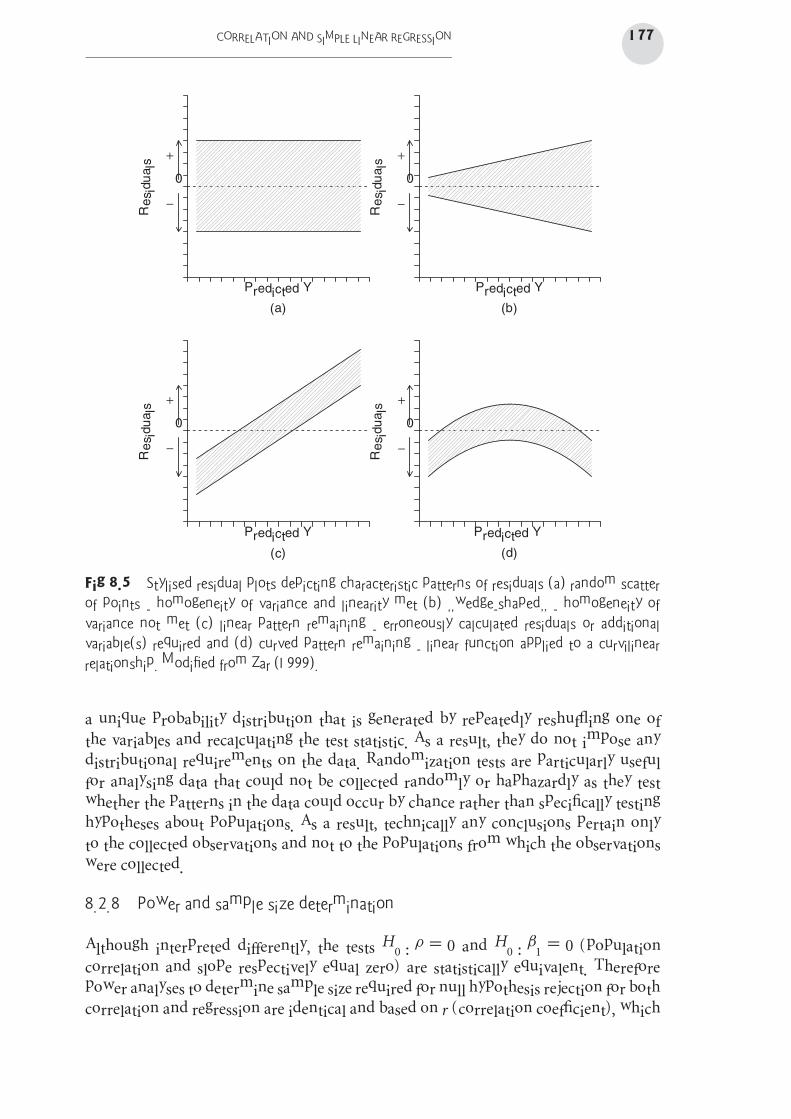
Fig 8.5 Stylised residual plots depicting characteristic patterns of residuals (a) random scatter
of points - homogeneity of variance and linearity met (b) ‘‘wedge-shaped’’ - homogeneity of
variance not met (c) linear pattern remaining - erroneously calculated residuals or additional
variable(s) required and (d) curved pattern remaining - linear function applied to a curvilinear
relationship. Modified from Zar (1999).
a unique probability distribution that is generated by repeatedly reshuffling one of
the variables and recalculating the test statistic. As a result, they do not impose any
distributional requirements on the data. Randomization tests are particularly useful
for analysing data that could not be collected randomly or haphazardly as they test
whether the patterns in the data could occur by chance rather than specifically testing
hypotheses about populations. As a result, technically any conclusions pertain only
to the collected observations and not to the populations from which the observations
were collected.
8.2.8 Power and sample size determination
Although interpreted differently, the tests H0 : ρ = 0 and H0 : β1 = 0 (population
correlation and slope respectively equal zero) are statistically equivalent. Therefore
power analyses to determine sample size required for null hypothesis rejection for both
correlation and regression are identical and based on r (correlation coefficient), which

178 CHAPTER 8
from regression analyses, can be obtained from the coefficient of determination (r2) or
as r = b�
�
x2/�
y2.
8.3 Smoothers and local regression
Smoothers fit simple models (such as linear regression) through successive localized
subsets of the data to describe the nature of relationships between a response variable
and one or more predictor variables for each point in a data cloud. Importantly, these
techniques do not require the data to conform to a particular global model structure
(e.g. linear, exponential, etc). Essentially, smoothers generate a line (or surface) through
the data cloud by replacing each observation with a new value that is predicted from
the subset of observations immediately surrounding the original observation. The
subset of neighbouring observations surrounding an observation is known as a band
or window and the larger the bandwidth, the greater the degree of smoothing.
Smoothers can be used as graphical representations as well as to model (local
regression) the nature of relationships between response and predictor variables in a
manner analogous to linear regression. Different smoothers differ in the manner by
which the predicted values are created.
• running medians (or less robust running means) generate predicted values that are the
medians of the responses in the bands surrounding each observation.
• loess and lowesse (locally weighted scatterplot smoothing) - fit least squares regression
lines to successive subsets of the observations weighted according to their distance from
the target observation and thus depict changes in the trends throughout the data cloud.
• kernel smoothers - new smoothed y-values are computed as the weighted averages of
points within a defined window (bandwidth) or neighbourhood of the original x-values.
Hence the bandwidth depends on the scale of the x-axis. Weightings are determined by the
type of kernel smoother specified, and for. Nevertheless, the larger the window, the greater
the degree of smoothing.
• splines - join together a series of polynomial fits that have been generated after the entire
data cloud is split up into a number of smaller windows, the widths of which determine
the smoothness of the resulting piecewise polynomial.
Whilst the above smoothers provide valuable exploratory tools, they also form the
basis of the formal model fitting procedures supported via generalized additive models
(GAMs, see chapter 17).
8.4 Correlation and regression in R
Simple correlation and regression in R are performed using the cor.test() and lm()
functions. The mblm() and rlm() functions offer a range of non-parametric regression
e Lowess and loess functions are similar in that they both fit linear models through localizations of
the data. They differ in in that loess uses weighted quadratic least squares and lowess uses weighted
linear least squares. They also differ in how they determine the data spanning (neighborhood of
points regression model fitted to), and in that loess smoothers can fit surfaces and thus accomodate
multivariate data.

CORRELATION AND SIMPLE LINEAR REGRESSION 179
Table 8.2 Smoothing function within R. For each of the following, DV is the response variable
within the data dataset. Smoothers are plotted on scatterplots by using the smoother function
as the response variable in the points() function (e.g. points(runmed(DV)~IV, data,
type=’l’)).
Smoothera Syntax
Running median > runmed(data$DV,k)
where k is an odd number that defines the bandwidth of the window
and if k omitted, defaults to either Turlach or Struetzle breaking
algorithms depending on data size (Turlack for larger)
Loess > loess(DV~IV1+IV2+..., data, span=0.75)
where IV1, IV2 represent one or more predictor variables and span
controls the degree of smoothing
Lowess > lowess(data$IV, data$DV, f=2/3)
where IV represents the predictor variable and f controls the degree of
smoothing
Kernel > ksmooth(data$IV, data$DV, kernel="normal",
bandwidth=0.5)
where IV represents the predictor variable, kernel represents the
smoothing kernel (box or normal) and bandwidth is the
smoothing bandwidth
> density(data$DV, bw="nrd0", adjust=1)
where IV represents the predictor variable and bw and adjust
‘‘nrd0’’ the smoothing bandwidth and course bandwidth multiplier
respectively. Information on the alternative smoothing bandwidth
selectors for gaussian (normal) windows is obtained by typing
?bw.nrd
Splines > data.spl<-smooth.spline(data$IV, data$DV, spar)
> points(y~x, data.spl, type=’l’)
where IV represents the predictor variable and spar is the smoothing
coeficient, typically between 0 and 1.
aNote, there are many other functions and packages that facilitate alternatives to the smoothing functions listed here.
alternatives. Model II regressions are facilitated via the lm.II() function and the
common smoothing functions available in R are described in Table 8.2.
8.5 Further reading
• Theory
Fowler, J., L. Cohen, and P. Jarvis. (1998). Practical statistics for field biology. John
Wiley & Sons, England.
Hollander, M., and D. A. Wolfe. (1999). Nonparametric statistical methods, 2nd
edition. John Wiley & Sons, New York.
Manly, B. F. J. (1991).Randomization andMonte Carlo methods in biology. Chapman
& Hall, London.

180 CHAPTER 8
Quinn, G. P., and K. J. Keough. (2002). Experimental design and data analysis for
biologists. Cambridge University Press, London.
Sokal, R., andF. J. Rohlf. (1997).Biometry, 3rd edition.W.H. Freeman, SanFrancisco.
Zar, G. H. (1999). Biostatistical methods. Prentice-Hall, New Jersey.
• Practical - R
Crawley, M. J. (2007). The R Book. John Wiley, New York.
Dalgaard, P. (2002). Introductory Statistics with R. Springer-Verlag, New York.
Fox, J. (2002). An R and S-PLUS Companion to Applied Regression. Sage Books.
Maindonald, J. H., and J. Braun. (2003). Data Analysis and Graphics Using R - An
Example-based Approach. Cambridge University Press, London.
8.6 Key for correlation and regression
1 a. Neither variable has been set (they are both measured) AND there is no implied
causality between the variables (Correlation) . . . . . . . . . . . . . . . . . . . . . . . . . . Go to 2
b. Either one of the variables has been specifically set (not measured) OR there is an
implied causality between the variables whereby one variable could influence the
other but the reverse is unlikely (Regression) . . . . . . . . . . . . . . . . . . . . . . . . . . Go to 4
2 a. Check parametric assumptions for correlation analysis
• Bivariate normality of the response/predictor variables - marginal scatterplot
boxplots
> library(car)
> scatterplot(V1 ~ V2, dataset)
where V1 and V2 are the continuous variables in the dataset data frame
• Linearity of data points on a scatterplot, trendline and lowess smoother
useful
> library(car)
> scatterplot(V1 ~ V2, dataset, reg.line = F)
where V1 and V2 are the continuous variables in the dataset data frame and
reg.line=F excludes the misleading regression line from the plot
Parametric assumptionsmet (Pearson correlation) . . . . . . . . . . . . . See Example 8A
> corr.test(~V1 + V2, data = dataset)
where V1 and V2 are the continuous variables in the dataset data frame
For a summary plot . . . . . . . . . . . . . . . . . . . . . . . . . . . . . . . . . . . . . . . . . . . . . . . . . Go to 12
b. Parametric assumptions NOT met or scale transformations (see Table 3.2) not
successful or inappropriate . . . . . . . . . . . . . . . . . . . . . . . . . . . . . . . . . . . . . . . . . . . Go to 3
3 a. Sample size between 7 and 30 (Spearman rank correlation) . . . . . . See Example 8B
> cor.test(~V1 + V2, data = dataset, method = "spearman")
where V1 and V2 are the continuous variables in the dataset data frame
For a summary plot . . . . . . . . . . . . . . . . . . . . . . . . . . . . . . . . . . . . . . . . . . . . . . . . . Go to 12
b. Sample size> 30 (Kendall’s tao correlation)
> cor.test(~V1 + V2, data = dataset, method = "kendall")

CORRELATION AND SIMPLE LINEAR REGRESSION 181
where V1 and V2 are the continuous variables in the dataset data frame
For a summary plot . . . . . . . . . . . . . . . . . . . . . . . . . . . . . . . . . . . . . . . . . . . . . . . . . Go to 12
4 a. Check parametric assumptions for regression analysis
• Normality of the response variable (and predictor variable if measured) -
marginal scatterplot boxplots
• Homogeneity of variance - spread of data around scatterplot trendline
• Linearity of data points on a scatterplot, trendline and lowess smoother useful
> library(car)
> scatterplot(DV ~ IV, dataset)
where DV and IV are response and predictor variables respectively in the dataset
data frameParametric assumptionsmet . . . . . . . . . . . . . . . . . . . . . . . . . . . . . . . . . . . . . . . . . Go to 5
b. Parametric assumptions NOT met or scale transformations (see Table 3.2) not
successful or inappropriate . . . . . . . . . . . . . . . . . . . . . . . . . . . . . . . . . . . . . . . . . . . Go to 7
5 a. Levels of predictor variable set (not measured) - no uncertainty in predictor
variable OR the primary aim of the analysis is:
• hypothesis testing (H0 : β1 = 0)
• generating a predictive model (y = β0 + β1x)
(Ordinary least squares (OLS) regression) . . . . . . . . . . . . . . . . . . . . . . . . . . . . . Go to 6
b. Levels of predictor variable NOT set (they are measured) AND the main aim
of the analysis is to estimate the population slope of the relationship (Model II
regression) . . . . . . . . . . . . . . . . . . . . . . . . . . . . . . . . . . . . . . . . . . . . . . . . . . See Example 8F
> library(biology)
> data.lm <- lm.II(DV ~ IV, christ, type = "RMA")
> summary(data.lm)
where DV and IV are response and predictor variables respectively in the dataset data
frame. type can be one of "MA", "RMA", "rMA" or "OLS". For type="rMA", it is also
possible to force a minimum response of zero (zero=T).
To produce a summary plot . . . . . . . . . . . . . . . . . . . . . . . . . . . . . . . . . . . . . . . . . . Go to 12
6 a. Single response value for each level of the predictor variable . . . . . . . . . . . . . . . . See
Examples 8C&8D
> dataset.lm <- lm(IV ~ DV, dataset)
> plot(dataset.lm)
> influence.measures(dataset.lm)
> summary(dataset.lm)
where DV and IV are response and predictor variables respectively in the dataset data
frame.
To get parameter confidence intervals f . . . . . . . . . . . . . . . . . . . . . . . . . . . . . . . . Go to 10
To predict new values of the response variable . . . . . . . . . . . . . . . . . . . . . . . . . Go to 11
To produce a summary plot . . . . . . . . . . . . . . . . . . . . . . . . . . . . . . . . . . . . . . . . . . Go to 12
b. Multiple response values for each level of the predictor variable . . . . . . . . . . . . . See
Examples 8E
> anova(lm(DV ~ IV + as.factor(IV), dataset))
f If there is uncertainty in the predictor variable, parameter confidence intervals might be inappro-
priate.

182 CHAPTER 8
• Pooled residual term
> dataset.lm <- lm(DV ~ IV, dataset)
> summary(dataset.lm)
• Non-pooled residual term
> dataset.lm <- aov(DV ~ IV + Error(as.factor(IV)), dataset)
> summary(dataset.lm)
> lm(DV ~ IV, dataset)
where DV and IV are response and predictor variables respectively in the dataset data
frame.
7 a. Observations collected randomly/haphazardly, no reason to suspect
non-independence . . . . . . . . . . . . . . . . . . . . . . . . . . . . . . . . . . . . . . . . . . . . . . . . . . . Go to 8
b. Random/haphazard sampling not possible, observations not necessarily indepen-
dent (Randomization test) . . . . . . . . . . . . . . . . . . . . . . . . . . . . . . . . . . . See Example 8H
> stat <- function(data, index) {
+ summary(lm(DV ~ IV, data))$coef[2, 3]
+ }
> rand.gen <- function(data, mle) {
+ out <- data
+ out$IV <- sample(out$IV, replace = F)
+ out
+ }
> library(boot)
> dataset.boot <- boot(dataset, stat, R = 5000,
+ sim = "parametric", ran.gen = rand.gen)
> plot(dataset.boot)
> dataset.boot
where DV and IV are response and predictor variables respectively in the dataset data
frame.
To get parameter confidence intervalsg . . . . . . . . . . . . . . . . . . . . . . . . . . . . . . . . Go to 10
To predict new values of the response variable . . . . . . . . . . . . . . . . . . . . . . . . . Go to 11
To produce a summary plot . . . . . . . . . . . . . . . . . . . . . . . . . . . . . . . . . . . . . . . . . . Go to 12
8 a. Mild non-normality duemainly to outliers (influential obseravations), data linear
(M-regression)
> library(MASS)
> data.rlm <- rlm(DV ~ IV, dataset)
where DV and IV are response and predictor variables respectively in the dataset data
frame.
To get parameter confidence intervalsh . . . . . . . . . . . . . . . . . . . . . . . . . . . . . . . . Go to 12
To predict new values of the response variable . . . . . . . . . . . . . . . . . . . . . . . . . Go to 11
To produce a summary plot . . . . . . . . . . . . . . . . . . . . . . . . . . . . . . . . . . . . . . . . . . Go to 10
g If there is uncertainty in the predictor variable, parameter confidence intervals might be inappro-
priate.h If there is uncertainty in the predictor variable, parameter confidence intervals might be inappro-
priate.

CORRELATION AND SIMPLE LINEAR REGRESSION 183
b. Data non-normal and/or non-linear . . . . . . . . . . . . . . . . . . . . . . . . . . . . . . . . . . Go to 9
9 a. Binary response (e.g. dead/alive, present/absent) . . . . . . Logistic Regression
chapter 17
b. Underlying distribution of response variable and residuals is known . . . . . . GLM
chapter 17
c. Data curvilinear . . . . . . . . . . . . . . . . . . . . . . . . . . . . . . . Non-linear regression chapter 9
d. Data monotonic non-linear (nonparametric regression) . . . . . . . . See Example 8G
• Theil-Sen single median (Kendall’s) robust regression
> library(mblm)
> data.mblm <- mblm(DV ~ IV, dataset, repeated = F)
> summary(data.mblm)
• Siegel repeated medians regression
> library(mblm)
> data.mblm <- mblm(DV ~ IV, dataset, repeated = T)
> summary(data.mblm)
where DV and IV are response and predictor variables respectively in the dataset data
frame.
To get parameter confidence intervalsi . . . . . . . . . . . . . . . . . . . . . . . . . . . . . . . . Go to 12
To predict new values of the response variable . . . . . . . . . . . . . . . . . . . . . . . . . Go to 11
To produce a summary plot . . . . . . . . . . . . . . . . . . . . . . . . . . . . . . . . . . . . . . . . . . Go to 10
10 Generating parameter confidence intervals . . . . . . . . . . . . . . . . . . See Example 8C&8G
> confint(model, level = 0.95)
where model is a fitted model
To get randomization parameter estimates and their confidence intervals . . . . . . . . See
Example 8H
> par.boot <- function(dataset, index) {
+ x <- dataset$ALT[index]
+ y <- dataset$HK[index]
+ model <- lm(y ~ x)
+ coef(model)
+ }
> dataset.boot <- boot(dataset, par.boot, R = 5000)
> boot.ci(dataset.boot, index = 2)
where dataset is the data.frame. The optional argument (R=5000) indicates 5000
randomizations and the optional argument (index=2) indicates which parameter to
generate confidence intervals for (y-intercept=1, slope=2). Note the use of the lm()
function for the parameter estimations and could be replaced by robust alternatives such as
rlm() or mblm().
11 Generating new response values (and corresponding prediction intervals) . . . . . See
Example 8C&8D
> predict(model, data.frame(IV = c()), interval = "p")
i If there is uncertainty in the predictor variable, parameter confidence intervals might be inappro-
priate.

184 CHAPTER 8
where model is a fitted model and IV is the predictor variable and c() is a vector of new
predictor values (e.g. c(10,13.4))
To get randomization prediction intervals . . . . . . . . . . . . . . . . . . . . . . . . See Example 8H
> pred.boot <- function(dataset, index) {
+ dataset.rs <- dataset[index, ]
+ dataset.lm <- lm(HK ~ ALT, dataset.rs)
+ predict(dataset.lm, data.frame(ALT = 1))
+ }
> dataset.boot <- boot(dataset, pred.boot, R = 5000)
> boot.ci(dataset.boot)
where dataset is the name of the data frame. Note the use of the lm() function for the
parameter estimations. This could be replaced by robust alternatives such as rlm() or
mblm().
12 Base summary plot for correlation or regression . . . . . . See Example 8B&8C&8D&8F
> plot(V1 ~ V2, data, pch = 16, axes = F, xlab = "", ylab = "")
> axis(1, cex.axis = 0.8)
> mtext(text = "x-axis title", side = 1, line = 3)
> axis(2, las = 1)
> mtext(text = "y-axis title", side = 2, line = 3)
> box(bty = "l")
where V1 and V2 are the continuous variables in the dataset data frame. For regression,
V1 represents the response variable and V2 represents the predictor variable.
Adding confidence ellipse . . . . . . . . . . . . . . . . . . . . . . . . . . . . . . . . . . . . . . . See Example 8B
> data.ellipse(V2, V1, levels = 0.95, add = T)
Adding regression line . . . . . . . . . . . . . . . . . . . . . . . . . . . . . . . . . . . . . . . . . . See Example 8C
> abline(model)
where model represents a fitted regression model
Adding regression confidence intervals . . . . . . . . . . . . . . . . . . . . . . See Example 8C&8D
> x <- seq(min(IV), max(IV), l = 1000)
> y <- predict(object, data.frame(IV = x), interval = "c")
> matlines(x, y, lty = 1, col = 1)
where IV is the name of the predictor variable (including the dataframe) model represents
a fitted regression model
8.7 Worked examples of real biological data sets
Example 8A: Pearson’s product moment correlation
Sokal and Rohlf (1997) present an unpublished data set (L. Miller) in which the correlation
between gill weight and body weight of the crab (Pachygrapsus crassipes) is investigated.
CORRELATION AND SIMPLE LINEAR REGRESSION 185
Step 1 - Import (section 2.3) the crabs data set
> crabs <- read.table("crabs.csv", header = T, sep = ",")
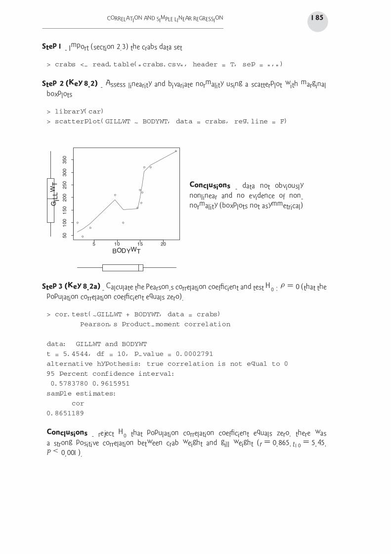
Step 2 (Key 8.2) - Assess linearity and bivariate normality using a scatterplot with marginal
boxplots
> library(car)
> scatterplot(GILLWT ~ BODYWT, data = crabs, reg.line = F)
5 10 15 20
50
100
150
200
250
300
350
BODYWT
GIL
LW
T
Conclusions - data not obviously
nonlinear and no evidence of non-
normality (boxplots not asymmetrical)
Step 3 (Key 8.2a) - Calculate the Pearson’s correlation coefficient and test H0 : ρ = 0 (that the
population correlation coefficient equals zero).
> cor.test(~GILLWT + BODYWT, data = crabs)
Pearson's product-moment correlation
data: GILLWT and BODYWT
t = 5.4544, df = 10, p-value = 0.0002791
alternative hypothesis: true correlation is not equal to 0
95 percent confidence interval:
0.5783780 0.9615951
sample estimates:
cor
0.8651189
Conclusions - reject H0 that population correlation coefficient equals zero, there was
a strong positive correlation between crab weight and gill weight (r = 0.865, t10 = 5.45,
P < 0.001).
186 CHAPTER 8
Example 8B: Spearman rank correlation
Green (1997) investigated the correlation between total biomass of red land crabs (Gecar-
coidea natalis and the density of their burrows at a number of forested sites (Lower site: LS
and Drumsite: DS) on Christmas Island.
Step 1 - Import (section 2.3) the Green (1997) data set
> green <- read.table("green.csv", header = T, sep = ",")
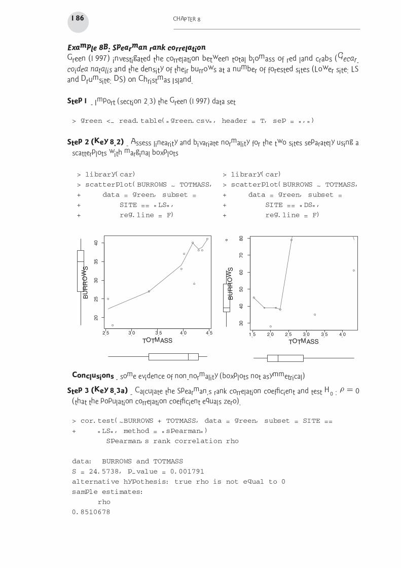
Step 2 (Key 8.2) - Assess linearity and bivariate normality for the two sites separately using a
scatterplots with marginal boxplots
> library(car)
> scatterplot(BURROWS ~ TOTMASS,
+ data = green, subset =
+ SITE == "LS",
+ reg.line = F)
20
25
30
35
40
TOTMASS
BU
RR
OW
S
2.5 3.0 3.5 4.0 4.5
> library(car)
> scatterplot(BURROWS ~ TOTMASS,
+ data = green, subset =
+ SITE == "DS",
+ reg.line = F)
30
40
50
60
70
80
TOTMASS
BU
RR
OW
S
1.5 2.0 2.5 3.0 3.5 4.0
Conclusions - some evidence of non-normality (boxplots not asymmetrical)
Step 3 (Key 8.3a) - Calculate the Spearman’s rank correlation coefficient and test H0 : ρ = 0
(that the population correlation coefficient equals zero).
> cor.test(~BURROWS + TOTMASS, data = green, subset = SITE ==
+ "LS", method = "spearman")
Spearman's rank correlation rho
data: BURROWS and TOTMASS
S = 24.5738, p-value = 0.001791
alternative hypothesis: true rho is not equal to 0
sample estimates:
rho
0.8510678
CORRELATION AND SIMPLE LINEAR REGRESSION 187
Conclusions - reject H0 that population correlation coefficient equals zero, there was a strong
positive correlation between crab biomass and burrow density at Low site (ρ = 0.851, S10 =
24.57, P = 0.0018).
> cor.test(~BURROWS + TOTMASS, data = green, subset = SITE ==
+ "DS", method = "spearman")
Spearman's rank correlation rho
data: BURROWS and TOTMASS
S = 69.9159, p-value = 0.6915
alternative hypothesis: true rho is not equal to 0
sample estimates:
rho
0.1676677
Conclusions - do not reject H0 that population correlation coefficient equals zero, there was
no detectable correlation between crab weight and gill weight at Drumsite (ρ = 0.168, S10 =
69.92, P = 0.692).
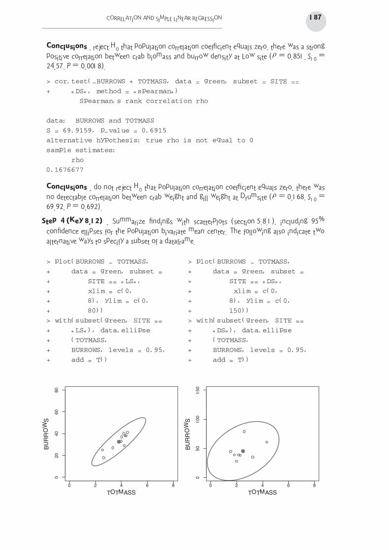
Step 4 (Key 8.12) - Summarize findings with scatterplots (section 5.8.1), including 95%
confidence ellipses for the population bivariate mean center. The following also indicate two
alternative ways to specify a subset of a dataframe.
> plot(BURROWS ~ TOTMASS,
+ data = green, subset =
+ SITE == "LS",
+ xlim = c(0,
+ 8), ylim = c(0,
+ 80))
> with(subset(green, SITE ==
+ "LS"), data.ellipse
+ (TOTMASS,
+ BURROWS, levels = 0.95,
+ add = T))
0 2 4 6 8
02
04
06
08
0
TOTMASS
BU
RR
OW
S
> plot(BURROWS ~ TOTMASS,
+ data = green, subset =
+ SITE == "DS",
+ xlim = c(0,
+ 8), ylim = c(0,
+ 150))
> with(subset(green, SITE ==
+ "DS"), data.ellipse
+ (TOTMASS,
+ BURROWS, levels = 0.95,
+ add = T))
0 2 4 6 8
50
01
00
15
0
TOTMASS
BU
RR
OW
S
188 CHAPTER 8
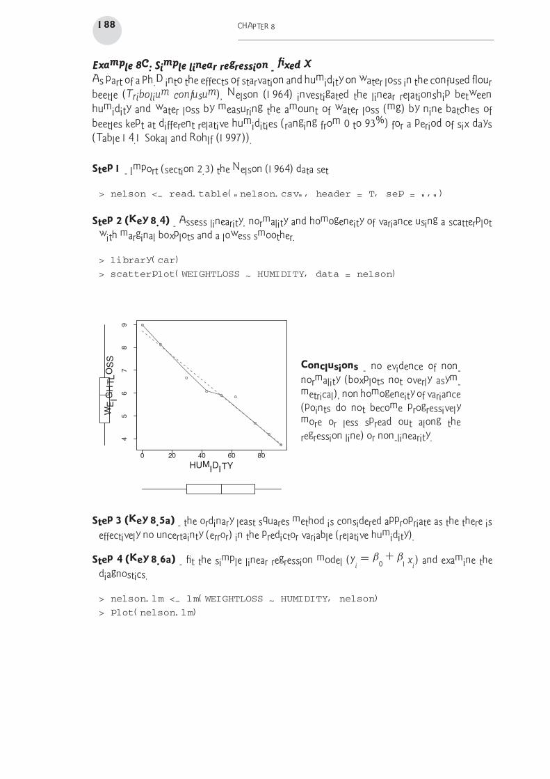
Example 8C: Simple linear regression - fixed X
As part of a Ph.D into the effects of starvation and humidity on water loss in the confused flour
beetle (Tribolium confusum), Nelson (1964) investigated the linear relationship between
humidity and water loss by measuring the amount of water loss (mg) by nine batches of
beetles kept at different relative humidities (ranging from 0 to 93%) for a period of six days
(Table 14.1 Sokal and Rohlf (1997)).
Step 1 - Import (section 2.3) the Nelson (1964) data set
> nelson <- read.table("nelson.csv", header = T, sep = ",")
Step 2 (Key 8.4) - Assess linearity, normality and homogeneity of variance using a scatterplot
with marginal boxplots and a lowess smoother.
> library(car)
> scatterplot(WEIGHTLOSS ~ HUMIDITY, data = nelson)
0 20 40 60 80
45
67
89
HUMIDITY
WE
IGH
TL
OS
S
Conclusions - no evidence of non-
normality (boxplots not overly asym-
metrical), non homogeneity of variance
(points do not become progressively
more or less spread out along the
regression line) or non-linearity.
Step 3 (Key 8.5a) - the ordinary least squares method is considered appropriate as the there is
effectively no uncertainty (error) in the predictor variable (relative humidity).
Step 4 (Key 8.6a) - fit the simple linear regression model (yi = β0 + β1xi) and examine the
diagnostics.
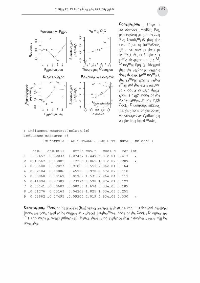
> nelson.lm <- lm(WEIGHTLOSS ~ HUMIDITY, nelson)
> plot(nelson.lm)
CORRELATION AND SIMPLE LINEAR REGRESSION 189
−0.4
0.0
0.4
Fitted values
Re
sid
ua
lsResiduals vs Fitted
3
6
4
−1.5 −0.5 0.5 1.5
−1.5
0.0
1.0
2.0
Theoretical QuantilesS
tan
da
rdiz
ed
resid
ua
ls
Normal Q-Q
3
6
1
0.0
0.4
0.8
1.2
Fitted values
Sta
nd
ard
ize
dre
sid
ua
ls
Scale-Location36
1
0.0 0.1 0.2 0.3 0.44 5 6 7 8
−2
−1
10
2
Leverage
Sta
nd
ard
ize
dre
sid
ua
ls
Cook’s distance 1
0.5
0.5
1
Residuals vs Leverage
1
3
6
4 5 6 7 8
Conclusions - There is
no obvious ‘‘wedge’’ pat-
tern evident in the residual
plot (confirming that the
assumption of homogene-
ity of variance is likely to
be met). Although there is
some deviation in the Q-
Q normal plot (suggesting
that the response variable
does deviate from normal),
the sample size is rather
small and the test is reason-
ably robust to such devia-
tions. Finally, none of the
points approach the high
Cook’s D contours suggest-
ing that none of the obser-
vations are overly influential
on the final fitted model.
> influence.measures(nelson.lm)
Influence measures of
lm(formula = WEIGHTLOSS ~ HUMIDITY, data = nelson) :
dfb.1_ dfb.HUMI dffit cov.r cook.d hat inf
1 1.07457 -0.92033 1.07457 1.449 5.31e-01 0.417 *
2 0.17562 -0.13885 0.17705 1.865 1.81e-02 0.289 *
3 -0.83600 0.52023 -0.91800 0.552 2.86e-01 0.164
4 -0.32184 0.10806 -0.45713 0.970 9.67e-02 0.118
5 0.00868 0.00169 0.01969 1.531 2.26e-04 0.112
6 0.11994 0.27382 0.73924 0.598 1.97e-01 0.129
7 0.00141 -0.00609 -0.00956 1.674 5.33e-05 0.187
8 -0.01276 0.03163 0.04208 1.825 1.03e-03 0.255
9 0.03662 -0.07495 -0.09204 2.019 4.93e-03 0.330 *
Conclusions - None of the leverage (hat) values are greater than 2 ∗ p/n = 0.444 and therefore
(none are considered to be outliers in x-space). Furthermore, none of the Cook’s D values are
≥ 1 (no point is overly influential). Hence there is no evidence that hypothesis tests will be
unreliable.
190 CHAPTER 8
Step 5 (Key 8.6a) - examine the parameter estimates and hypothesis tests (Boxes 14.1 & 14.3
of Sokal and Rohlf (1997)).
> summary(nelson.lm)
Call:
lm(formula = WEIGHTLOSS ~ HUMIDITY, data = nelson)
Residuals:
Min 1Q Median 3Q Max
-0.46397 -0.03437 0.01675 0.07464 0.45236
Coefficients:
Estimate Std. Error t value Pr(>|t|)
(Intercept) 8.704027 0.191565 45.44 6.54e-10 ***
HUMIDITY -0.053222 0.003256 -16.35 7.82e-07 ***
---
Signif. codes: 0 '***' 0.001 '**' 0.01 '*' 0.05 '.' 0.1 ' ' 1
Residual standard error: 0.2967 on 7 degrees of freedom
Multiple R-squared: 0.9745, Adjusted R-squared: 0.9708
F-statistic: 267.2 on 1 and 7 DF, p-value: 7.816e-07
Conclusions - Reject H0 that the population slope equals zero. An increase in relative humidity
was found to be associated with a strong (r2 = 0.975), significant decrease in weight loss
(b = −0.053, t7 = −16.35, P < 0.001) in confused flour beetles.
Step 6 (Key 8.10) - calculate the 95% confidence limits for the regression coefficients (Box
14.3 of Sokal and Rohlf (1997)).
> confint(nelson.lm)
2.5 % 97.5 %
(Intercept) 8.25104923 9.15700538
HUMIDITY -0.06092143 -0.04552287
Step 7 (Key 8.11) - use the fitted linear model to predict the mean weight loss of flour beetles
expected at 50 and 100% relative humidity (Box 14.3 of Sokal and Rohlf (1997)).
> predict(nelson.lm, data.frame(HUMIDITY = c(50, 100)),
+ interval = "prediction", se = T)
$fit
fit lwr upr
1 6.042920 5.303471 6.782368
2 3.381812 2.549540 4.214084
$se.fit
1 2
0.0988958 0.1894001
CORRELATION AND SIMPLE LINEAR REGRESSION 191
$df
[1] 7
$residual.scale
[1] 0.2966631
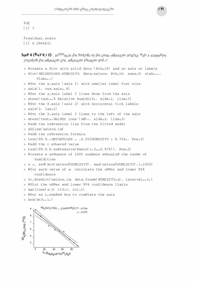
Step 8 (Key 8.12) - summarize the findings of the linear regression analysis with a scatterplot
including the regression line, regression equation and r2.
> #create a plot with solid dots (pch=16) and no axis or labels
> plot(WEIGHTLOSS~HUMIDITY, data=nelson, pch=16, axes=F, xlab="",
ylab="")
> #put the x-axis (axis 1) with smaller label font size
> axis(1, cex.axis=.8)
> #put the x-axis label 3 lines down from the axis
> mtext(text="% Relative humidity", side=1, line=3)
> #put the y-axis (axis 2) with horizontal tick labels
> axis(2, las=1)
> #put the y-axis label 3 lines to the left of the axis
> mtext(text="Weight loss (mg)", side=2, line=3)
> #add the regression line from the fitted model
> abline(nelson.lm)
> #add the regression formula
> text(99,9,"WEIGHTLOSS = -0.053HUMIDITY + 8.704", pos=2)
> #add the r squared value
> text(99,8.6,expression(paste(r^2==0.975)), pos=2)
> #create a sequence of 1000 numbers spanning the range of
humidities
> x <- seq(min(nelson$HUMIDITY), max(nelson$HUMIDITY),l=1000)
> #for each value of x, calculate the upper and lower 95%
confidence
> y<-predict(nelson.lm, data.frame(HUMIDITY=x), interval="c")
> #plot the upper and lower 95% confidence limits
> matlines(x,y, lty=1, col=1)
> #put an L-shaped box to complete the axis
> box(bty="l")
% Relative humidity
4
0 20 40 60 80
5
6
7
8
9
We
igh
t lo
ss (
mg
)
WEIGHTLOSS = −0.053HUMIDITY + 8.704
r2 = 0.975
192 CHAPTER 8
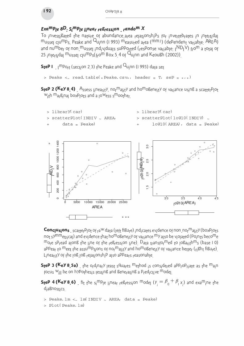
Example 8D: Simple linear regression - random X
To investigated the nature of abundance-area relationships for invertebrates in intertidal
mussel clumps, Peake and Quinn (1993) measured area (mm2) (dependent variable: AREA)
and number of non-mussel individuals supported (response variable: INDIV) from a total of
25 intertidal mussel clumps(from Box 5.4 of Quinn and Keough (2002)).
Step 1 - Import (section 2.3) the Peake and Quinn (1993) data set
> peake <- read.table("peake.csv", header = T, sep = ",")
Step 2 (Key 8.4) - Assess linearity, normality and homogeneity of variance using a scatterplot
with marginal boxplots and a lowess smoother.
> library(car)
> scatterplot(INDIV ~ AREA,
+ data = peake)
0 5000 10000 15000 20000 25000
02
00
40
06
00
80
01
00
01
20
01
40
0
AREA
IND
IV
> library(car)
> scatterplot(log10(INDIV) ~
+ log10(AREA), data = peake)
3.0 3.5 4.0 4.5
1.5
2.0
2.5
3.0
log10(AREA)
log10(I
ND
IV)
Conclusions - scatterplot of raw data (left figure) indicates evidence of non-normality (boxplots
not symmetrical) and evidence that homogeneity of variance my also be violated (points become
more spread along the line of the regression line). Data transformed to logarithms (base 10)
appear to meet the assumptions of normality and homogeneity of variance better (right figure).
Linearity of the log-log relationship also appears reasonable.
Step 3 (Key 8.5a) - the ordinary least squares method is considered appropriate as the main
focus will be on hypothesis testing and generating a predictive model.
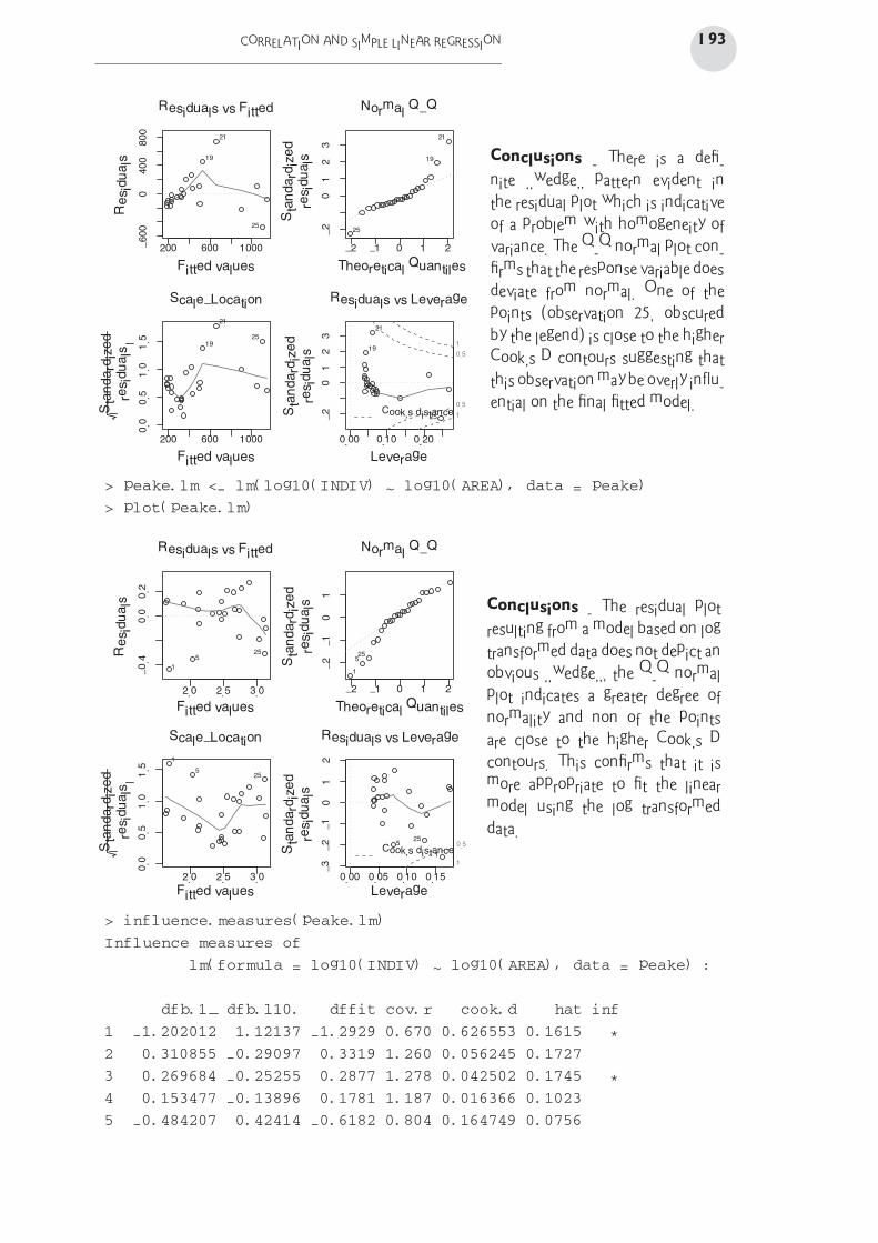
Step 4 (Key 8.6) - fit the simple linear regression model (yi = β0 + β1xi) and examine the
diagnostics.
> peake.lm <- lm(INDIV ~ AREA, data = peake)
> plot(peake.lm)
CORRELATION AND SIMPLE LINEAR REGRESSION 193
200 600 1000
−6
00
04
00
80
0
Fitted values
Re
sid
ua
lsResiduals vs Fitted
21
25
19
−2 −1 210
−2
32
10
Theoretical Quantiles
Sta
nd
ard
ize
dre
sid
ua
ls
Normal Q−Q
21
25
19
200 600 1000
0.0
0.5
1.0
1.5
Fitted values
Scale−Location21
2519
0.00 0.10 0.20
Leverage
Sta
nd
ard
ize
dre
sid
ua
ls
Cook’s distance 1
0.5
0.5
1
Residuals vs Leverage
25
21
19
Sta
nd
ard
ize
dre
sid
ua
ls
32
10
−2
Conclusions - There is a defi-
nite ‘‘wedge’’ pattern evident in
the residual plot which is indicative
of a problem with homogeneity of
variance. The Q-Q normal plot con-
firms that the response variable does
deviate from normal. One of the
points (observation 25, obscured
by the legend) is close to the higher
Cook’s D contours suggesting that
this observation may be overly influ-
ential on the final fitted model.
> peake.lm <- lm(log10(INDIV) ~ log10(AREA), data = peake)
> plot(peake.lm)
2.0 2.5 3.0
−0
.40
.00
.2
Residuals vs Fitted
1
525
−2
−1
01
Normal Q−Q
1
525
2.0 2.5 3.0
0.0
0.5
1.0
1.5
1
525
0.00 0.05 0.10 0.15
−3
−2
−1
01
2
Cook’s distance1
0.5
1
255
Re
sid
ua
ls
Sta
nd
ard
ize
dre
sid
ua
lsS
tan
da
rdiz
ed
resid
ua
ls
Sta
nd
ard
ize
dre
sid
ua
ls
Fitted values Theoretical Quantiles
Fitted values
Scale−Location
Leverage
Residuals vs Leverage
−2 −1 210
Conclusions - The residual plot
resulting from a model based on log
transformed data does not depict an
obvious ‘‘wedge’’, the Q-Q normal
plot indicates a greater degree of
normality and non of the points
are close to the higher Cook’s D
contours. This confirms that it is
more appropriate to fit the linear
model using the log transformed
data.
> influence.measures(peake.lm)
Influence measures of
lm(formula = log10(INDIV) ~ log10(AREA), data = peake) :
dfb.1_ dfb.l10. dffit cov.r cook.d hat inf
1 -1.202012 1.12137 -1.2929 0.670 0.626553 0.1615 *
2 0.310855 -0.29097 0.3319 1.260 0.056245 0.1727
3 0.269684 -0.25255 0.2877 1.278 0.042502 0.1745 *
4 0.153477 -0.13896 0.1781 1.187 0.016366 0.1023
5 -0.484207 0.42414 -0.6182 0.804 0.164749 0.0756
194 CHAPTER 8
6 -0.062392 0.05251 -0.0897 1.151 0.004183 0.0608
7 0.052830 -0.04487 0.0739 1.158 0.002846 0.0633
8 0.187514 -0.15760 0.2707 1.052 0.036423 0.0605
9 0.006384 -0.00416 0.0164 1.141 0.000140 0.0428
10 0.004787 -0.00131 0.0244 1.137 0.000311 0.0401
11 0.013583 0.00419 0.1238 1.101 0.007882 0.0400
12 -0.003011 -0.00112 -0.0287 1.137 0.000432 0.0401
13 0.000247 0.00259 0.0198 1.138 0.000204 0.0407
14 -0.003734 -0.00138 -0.0356 1.135 0.000662 0.0401
15 -0.015811 0.05024 0.2419 1.013 0.028826 0.0418
16 -0.017200 0.02518 0.0595 1.142 0.001842 0.0487
17 -0.061445 0.09368 0.2375 1.038 0.028033 0.0474
18 -0.025317 0.03314 0.0619 1.151 0.001995 0.0561
19 -0.146377 0.18521 0.3173 1.015 0.049144 0.0607
20 0.100361 -0.13065 -0.2406 1.064 0.028981 0.0567
21 -0.263549 0.31302 0.4496 0.963 0.095261 0.0776
22 0.263206 -0.29948 -0.3786 1.101 0.071044 0.1069
23 0.043182 -0.04845 -0.0588 1.246 0.001804 0.1248
24 0.167829 -0.18726 -0.2236 1.226 0.025747 0.1341
25 0.545842 -0.61039 -0.7334 0.929 0.241660 0.1302
Conclusions - Whilst three leverage (hat) values are greater than 2 ∗ p/n = 0.16 (obser-
vations 1, 2 and 3) and therefore potentially outliers in x-space, none of the Cook’s D
values are ≥ 1 (no point is overly influential). No evidence that hypothesis tests will be
unreliable.
Step 5 (Key 8.6a) - examine the parameter estimates and hypothesis tests.
> summary(peake.lm)
Call:
lm(formula = log10(INDIV) ~ log10(AREA), data = peake)
Residuals:
Min 1Q Median 3Q Max
-0.43355 -0.06464 0.02219 0.11178 0.26818
Coefficients:
Estimate Std. Error t value Pr(>|t|)
(Intercept) -0.57601 0.25904 -2.224 0.0363 *
log10(AREA) 0.83492 0.07066 11.816 3.01e-11 ***
---
Signif. codes: 0 '***' 0.001 '**' 0.01 '*' 0.05 '.' 0.1 ' ' 1
Residual standard error: 0.1856 on 23 degrees of freedom
Multiple R-squared: 0.8586, Adjusted R-squared: 0.8524
F-statistic: 139.6 on 1 and 23 DF, p-value: 3.007e-11
CORRELATION AND SIMPLE LINEAR REGRESSION 195
Conclusions - Reject H0 that the population slope equals zero. An increase in (log) mussel
clump area was found to be associated with a strong (r2 = 0.859), significant increase in the
(log) number of supported invertebrate individuals (b = 0.835, t23 = 11.816, P < 0.001).
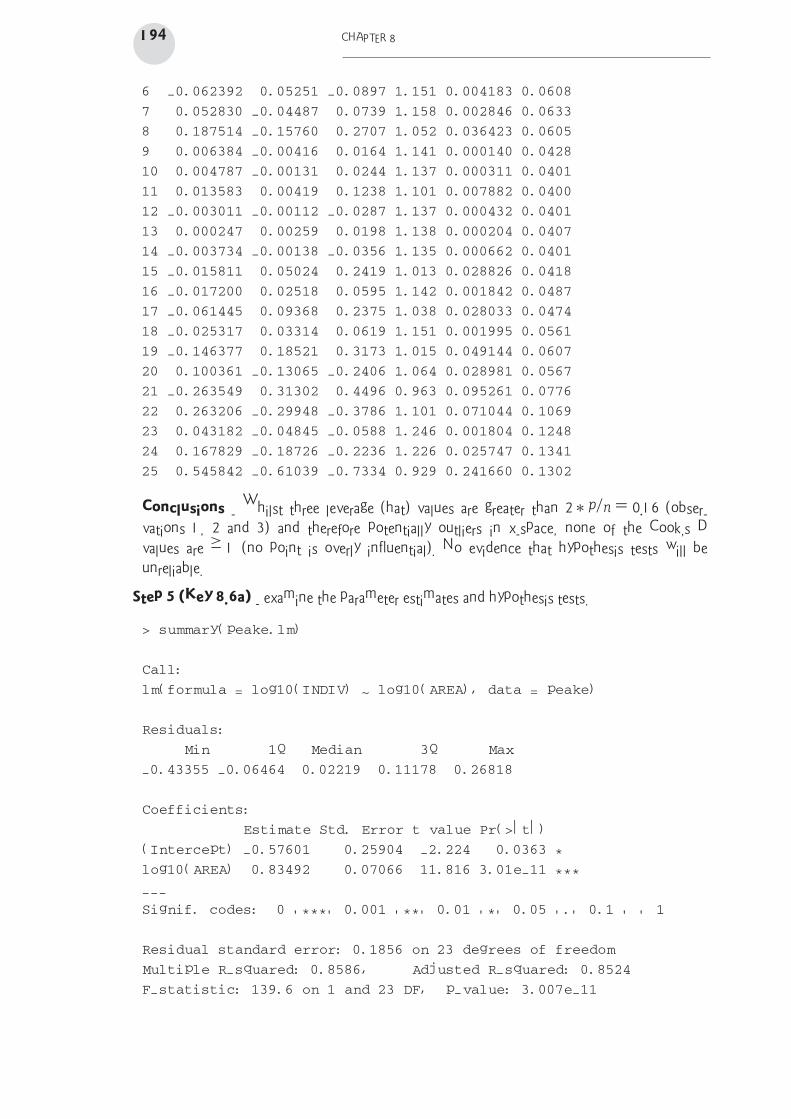
Step 6 (Key 8.12) - summarize the findings of the linear regression analysis with a scatterplot
including the regression line, regression equation and r2.
> #create a plot with solid dots (pch=16) and no axis or labels}
> plot(INDIV~AREA, data=peake, pch=16, axes=F, xlab="", ylab="",
log="xy")
> #put the x-axis (axis 1) with smaller label font size
> axis(1, cex.axis=.8)
> #put the x-axis label 3 lines down from the axis
> mtext(text=expression(paste("Mussel clump area", (mm^2))),
side=1, line=3)
> #put the y-axis (axis 2) with horizontal tick labels
> axis(2, las=1)
> #put the y-axis label 3 lines to the left of the axis
> mtext(text="Number of individuals", side=2, line=3)
> #add the regression line from the fitted model
> abline(peake.lm)
> #add the regression formula
> text(30000, 30, expression(paste(log[10], "INDIV = 0.835",
+ log[10], "AREA - 0.576")), pos=2)
> #add the r squared value
> text(30000, 22, expression(paste(r^2==0.835)), pos=2)
> #put an L-shaped box to complete the axis
> box(bty="l")
500 1000 2000 5000 10000 20000
Mussel clump area(mm2)
20
50
100
200
500
1000
Nu
mb
er
of
ind
ivid
ua
ls
log10INDIV = 0.835log10AREA – 0.576
r2 = 0.835
Step 7 (Key 8.11) - use the fitted linear model to predict the number of individuals that would
be supported on two new mussel clumps with areas of 8000 and 10000 mm2.
> 10^predict(peake.lm, data.frame(AREA = c(8000, 10000)))
1 2
481.6561 580.2949
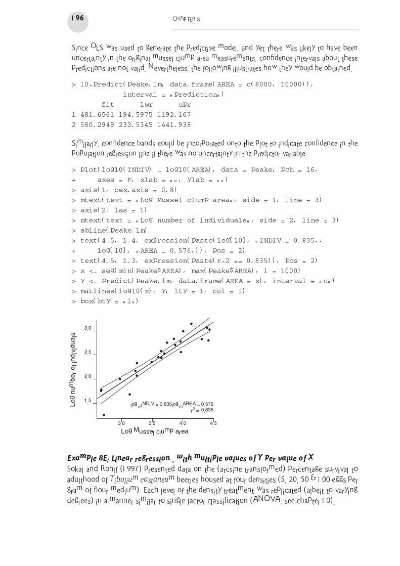
196 CHAPTER 8
Since OLS was used to generate the predictive model, and yet there was likely to have been
uncertainty in the original mussel clump area measurements, confidence intervals about these
predictions are not valid. Nevertheless, the following illustrates how they would be obtained.
> 10^predict(peake.lm, data.frame(AREA = c(8000, 10000)),
interval = "prediction")
fit lwr upr
1 481.6561 194.5975 1192.167
2 580.2949 233.5345 1441.938
Similarly, confidence bands could be incorporated onto the plot to indicate confidence in the
population regression line if there was no uncertainty in the predictor variable.
> plot(log10(INDIV) ~ log10(AREA), data = peake, pch = 16,
+ axes = F, xlab = "", ylab = "")
> axis(1, cex.axis = 0.8)
> mtext(text = "Log Mussel clump area", side = 1, line = 3)
> axis(2, las = 1)
> mtext(text = "Log number of individuals", side = 2, line = 3)
> abline(peake.lm)
> text(4.5, 1.4, expression(paste(log[10], "INDIV = 0.835",
+ log[10], "AREA - 0.576")), pos = 2)
> text(4.5, 1.3, expression(paste(r^2 == 0.835)), pos = 2)
> x <- seq(min(peake$AREA), max(peake$AREA), l = 1000)
> y <- predict(peake.lm, data.frame(AREA = x), interval = "c")
> matlines(log10(x), y, lty = 1, col = 1)
> box(bty = "l")
3.0 3.5 4.0 4.5
Log Mussel clump area
1.5
2.0
2.5
3.0
Lo
g n
um
be
r o
f in
div
idu
als
log10INDIV = 0.835log10AREA – 0.576 r2 = 0.835
Example 8E: Linear regression - with multiple values of Y per value of X
Sokal and Rohlf (1997) presented data on the (arcsine transformed) percentage survival to
adulthood of Tibolium castaneum beetles housed at four densities (5, 20, 50 & 100 eggs per
gram of flour medium). Each level of the density treatment was replicated (albeit to varying
degrees) in a manner similar to single factor classification (ANOVA, see chapter 10).
CORRELATION AND SIMPLE LINEAR REGRESSION 197
Step 1 - Import (section 2.3) the beetles data set
> beetles <- read.table("beetles.csv", header = T, sep = ",")
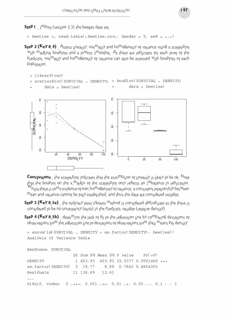
Step 2 (Key 8.4) - Assess linearity, normality and homogeneity of variance using a scatterplot
with marginal boxplots and a lowess smoother. As there are replicates for each level of the
predictor, normality and homogeneity of variance can also be assessed with boxplots of each
population.
> library(car)
> scatterplot(SURVIVAL ~ DENSITY,
+ data = beetles)
20 40 60 80 100
50
55
60
65
70
DENSITY
SU
RV
IVA
L
> boxplot(SURVIVAL ~ DENSITY,
+ data = beetles)
5 20 50 100
50
55
60
65
70
Conclusions - the scatterplot indicates that the assumption of linearity is likely to be ok. Note
that the boxplot on the x-margin of the scatterplot only reflects an imbalance in replication.
Whilst there is some evidence of non-homogeniety of variance, a consistent relationship between
mean and variance cannot be fully established, and thus the data are considered suitable.
Step 3 (Key 8.5a) - the ordinary least squares method is considered appropriate as the there is
considered to be no uncertainty (error) in the predictor variable (relative density).
Step 4 (Key 8.5b) - determine the lack of fit to the regression line by comparing deviations of
observations from the regression line to deviations of observations from their means per density.
> anova(lm(SURVIVAL ~ DENSITY + as.factor(DENSITY), beetles))
Analysis of Variance Table
Response: SURVIVAL
Df Sum Sq Mean Sq F value Pr(>F)
DENSITY 1 403.93 403.93 32.0377 0.0001466 ***
as.factor(DENSITY) 2 19.77 9.89 0.7842 0.4804305
Residuals 11 138.69 12.61
---
Signif. codes: 0 '***' 0.001 '**' 0.01 '*' 0.05 '.' 0.1 ' ' 1
198 CHAPTER 8
Conclusions - deviations from linear not significantly different from zero (F = 0.7842, P =
0.480), hence there is no evidence that a straight line is not an adequate representation of these
data.
Step 5 (Key 8.5b) - consider whether to pool deviations from the regression line and the
deviations from the predictor level means
> #calculate critical F for alpha=0.25, df=2,11
> qf(0.25,2,11, lower=T)
[1] 0.2953387
Conclusions - Sokal and Rohlf (1997) suggest that while there is no difference between the
deviations from the regression line and the deviations from the predictor level means, they
should not be pooled because F = 0.784 > F0.75[2,11] = 0.295.
Step 6 (Key 8.5b) - to test whether the regression is linear by comparing the fit of the linear
regression with the deviations from linearity (non pooled).
> beetles.lm <- aov(SURVIVAL ~ DENSITY + Error(as.factor(DENSITY)),
+ beetles)
> summary(beetles.lm)
Error: as.factor(DENSITY)
Df Sum Sq Mean Sq F value Pr(>F)
DENSITY 1 403.93 403.93 40.855 0.02361 *
Residuals 2 19.77 9.89
---
Signif. codes: 0 '***' 0.001 '**' 0.01 '*' 0.05 '.' 0.1 ' ' 1
Error: Within
Df Sum Sq Mean Sq F value Pr(>F)
Residuals 11 138.687 12.608
Conclusions - Reject H0 that the population is not linear.
> #to get the regression coefficients
> lm(SURVIVAL~DENSITY, beetles)
Call:
lm(formula = SURVIVAL ~ DENSITY, data = beetles)
Coefficients:
(Intercept) DENSITY
65.960 -0.147
If we had decided to pool, the analysis could have been performed as follows:
> summary(lm(SURVIVAL ~ DENSITY, beetles))
Call:
lm(formula = SURVIVAL ~ DENSITY, data = beetles)
CORRELATION AND SIMPLE LINEAR REGRESSION 199
Residuals:
Min 1Q Median 3Q Max
-6.8550 -1.8094 -0.2395 2.7856 5.1902
Coefficients:
Estimate Std. Error t value Pr(>|t|)
(Intercept) 65.96004 1.30593 50.508 2.63e-16 ***
DENSITY -0.14701 0.02554 -5.757 6.64e-05 ***
---
Signif. codes: 0 '***' 0.001 '**' 0.01 '*' 0.05 '.' 0.1 ' ' 1
Residual standard error: 3.491 on 13 degrees of freedom
Multiple R-squared: 0.7182, Adjusted R-squared: 0.6966
F-statistic: 33.14 on 1 and 13 DF, p-value: 6.637e-05
Note that these data could also have been analysed as a single factor ANOVA with polynomial
contrasts
> beetles$DENSITY <- as.factor(beetles$DENSITY)
> contrasts(beetles$DENSITY) <- contr.poly(4, c(5, 20, 50,
+ 100))
> beetles.aov <- aov(SURVIVAL ~ DENSITY, beetles)
> summary(beetles.aov, split = list(DENSITY = list(1, c(2,
+ 3))))
Df Sum Sq Mean Sq F value Pr(>F)
DENSITY 3 423.70 141.23 11.2020 0.0011367 **
DENSITY: C1 1 403.93 403.93 32.0377 0.0001466 ***
DENSITY: C2 2 19.77 9.89 0.7842 0.4804305
Residuals 11 138.69 12.61
---
Signif. codes: 0 '***' 0.001 '**' 0.01 '*' 0.05 '.' 0.1 ' ' 1
Example 8F: Model II regression
To contrast the parameter estimates resulting from model II regression, Quinn and Keough
(2002) used a data set from Christensen et al. (1996) (Box 5.7 Quinn and Keough (2002)).
Whilst model II regression is arguably unnecessary for these data (as it is hard to imagine
why estimates of the regression parameters would be the sole interest of the Christensen
et al. (1996) investigation), we will proceed with the aim of gaining a reliable estimate of the
population slope is required.
Step 1 - Import (section 2.3) the Christensen et al. (1996) data set
> christ <- read.table("christ.csv", header = T, sep = ",")
200 CHAPTER 8
Step 2 (Key 8.4) - Assess linearity, normality and homogeneity of variance using a scatterplot
with marginal boxplots and a lowess smoother.
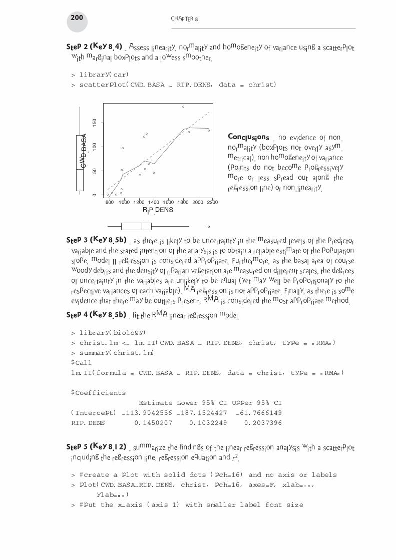
> library(car)
> scatterplot(CWD.BASA ~ RIP.DENS, data = christ)
800 1000 1200 1400 1600 1800 2000 2200
050
100
150
RIP.DENS
CW
D.B
AS
A
Conclusions - no evidence of non-
normality (boxplots not overly asym-
metrical), non homogeneity of variance
(points do not become progressively
more or less spread out along the
regression line) or non-linearity.
Step 3 (Key 8.5b) - as there is likely to be uncertainty in the measured levels of the predictor
variable and the stated intention of the analysis is to obtain a reliable estimate of the population
slope, model II regression is considered appropriate. Furthermore, as the basal area of course
woody debris and the density of riparian vegetation are measured on different scales, the degrees
of uncertainty in the variables are unlikely to be equal (yet may well be proportionaly to the
respective variances of each variable), MA regression is not appropriate. Finally, as there is some
evidence that there may be outliers present, RMA is considered the most appropriate method.
Step 4 (Key 8.5b) - fit the RMA linear regression model.
> library(biology)
> christ.lm <- lm.II(CWD.BASA ~ RIP.DENS, christ, type = "RMA")
> summary(christ.lm)
$Call
lm.II(formula = CWD.BASA ~ RIP.DENS, data = christ, type = "RMA")
$Coefficients
Estimate Lower 95% CI Upper 95% CI
(Intercept) -113.9042556 -187.1524427 -61.7666149
RIP.DENS 0.1450207 0.1032249 0.2037396
Step 5 (Key 8.12) - summarize the findings of the linear regression analysis with a scatterplot
including the regression line, regression equation and r2.
> #create a plot with solid dots (pch=16) and no axis or labels
> plot(CWD.BASA~RIP.DENS, christ, pch=16, axes=F, xlab="",
ylab="")
> #put the x-axis (axis 1) with smaller label font size
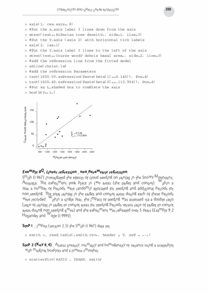
CORRELATION AND SIMPLE LINEAR REGRESSION 201
> axis(1, cex.axis=.8)
> #put the x-axis label 3 lines down from the axis
> mtext(text="Riparian tree density", side=1, line=3)
> #put the y-axis (axis 2) with horizontal tick labels
> axis(2, las=1)
> #put the y-axis label 3 lines to the left of the axis
> mtext(text="Course woody debris basal area", side=2, line=3)
> #add the regression line from the fitted model
> abline(christ.lm)
> #add the regression parameters
> text(1600,50,expression(paste(beta[1]==0.145)), pos=4)
> text(1600,40,expression(paste(beta[0]==-113.904)), pos=4)
> #put an L-shaped box to complete the axis
> box(bty="l")
800 1000 1200 1400 1600 1800 2000 2200
Riparian tree density
0
50
100
150
Cours
e w
oody d
ebris b
asal are
a
β1 = 0.145β0 = −113.904
Example 8G: Linear regression - non-parametric regression
Smith (1967) investigated the effects of cloud seeding on rainfall in the Snowy Mountains,
Australia. The experiment took place in two areas (the target and control). Within a
year a number of periods were randomly allocated for seeding and additional periods for
non-seeding. The total rainfall in the target and control areas during each of these periods
were recorded. Within a single year, the impact of seeding was assessed via a double ratio
(ratio of rainfall in target to control areas for seeding periods versus ratio of target to control
areas during non-seeding times) and the experiment was repeated over 5 years (Example 9.2
Hollander and Wolfe (1999)).
Step 1 - Import (section 2.3) the Smith (1967) data set
> smith <- read.table("smith.csv", header = T, sep = ",")
Step 2 (Key 8.4) - Assess linearity, normality and homogeneity of variance using a scatterplot
with marginal boxplots and a lowess smoother.
> scatterplot(RATIO ~ YEARS, smith)
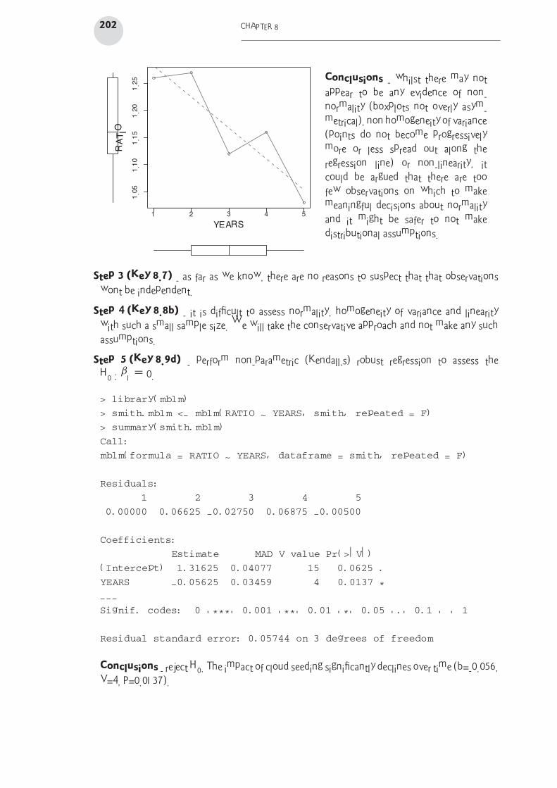
202 CHAPTER 8
1
1.0
51.1
01.1
51
.20
1.2
5
YEARS
RA
TIO
2 3 4 5
Conclusions - whilst there may not
appear to be any evidence of non-
normality (boxplots not overly asym-
metrical), non homogeneity of variance
(points do not become progressively
more or less spread out along the
regression line) or non-linearity, it
could be argued that there are too
few observations on which to make
meaningful decisions about normality
and it might be safer to not make
distributional assumptions.
Step 3 (Key 8.7) - as far as we know, there are no reasons to suspect that that observations
wont be independent.
Step 4 (Key 8.8b) - it is difficult to assess normality, homogeneity of variance and linearity
with such a small sample size. We will take the conservative approach and not make any such
assumptions.
Step 5 (Key 8.9d) - perform non-parametric (Kendall’s) robust regression to assess the
H0 : β1 = 0.
> library(mblm)
> smith.mblm <- mblm(RATIO ~ YEARS, smith, repeated = F)
> summary(smith.mblm)
Call:
mblm(formula = RATIO ~ YEARS, dataframe = smith, repeated = F)
Residuals:
1 2 3 4 5
0.00000 0.06625 -0.02750 0.06875 -0.00500
Coefficients:
Estimate MAD V value Pr(>|V|)
(Intercept) 1.31625 0.04077 15 0.0625 .
YEARS -0.05625 0.03459 4 0.0137 *
---
Signif. codes: 0 '***' 0.001 '**' 0.01 '*' 0.05 '.' 0.1 ' ' 1
Residual standard error: 0.05744 on 3 degrees of freedom
Conclusions - reject H0. The impact of cloud seeding significantly declines over time (b=-0.056,
V=4, P=0.0137).

CORRELATION AND SIMPLE LINEAR REGRESSION 203
Step 6 (Key 8.10) - calculate 95% confidence intervals for the parameter estimates.
> confint.mblm(smith.mblm, level = 0.95)
0.025 0.975
(Intercept) 1.28875 1.385
YEARS -0.10000 -0.015
Example 8H: Linear regression - randomization test
McKechnie et al. (1975) investigated the relationship between altitude and the frequency of
hezokinase (HK) 1.00 mobility genes from colonies of Euphydras editha butterflies (Example
8.1 Manly (1991)).
Step 1 - Import (section 2.3) the McKechnie et al. (1975) data set
> mckechnie <- read.table("mckechnie.csv", header = T, sep = ",")
Step 2 (Key 8.4) - Assess linearity, normality and homogeneity of variance using a scatterplot
with marginal boxplots and a lowess smoother. For the purpose of this demonstration, lets
assume that the assumption of normality could not be met and more importantly, that the
observations are not independent, thereby necessitating an alternative regression method.
Step 3 (Key 8.7b) - use randomization to test whether the observed trend could be due to
chance.
1. define the statisticj to use in the randomization test - in this case the t-statistic
> stat <- function(data, index) {
+ summary(lm(HK ~ ALT, data))$coef[2, 3]
+ }
2. define how the data should be randomized - randomize the pairing of predictor and responses
(shuffle without replacement the predictor values amongst observations)
> rand.gen <- function(data, mle) {
+ out <- data
+ out$ALT <- sample(out$ALT, replace = F)
+ out
+ }
3. call a bootstrapping procedure to randomize 5000 times (this can take some time)
> library(boot)
j Consistent with Manly (1991), I have used OLS to estimate the regression parameters. However,
these parameters could alternatively be RMA or non-parametric regression estimates.
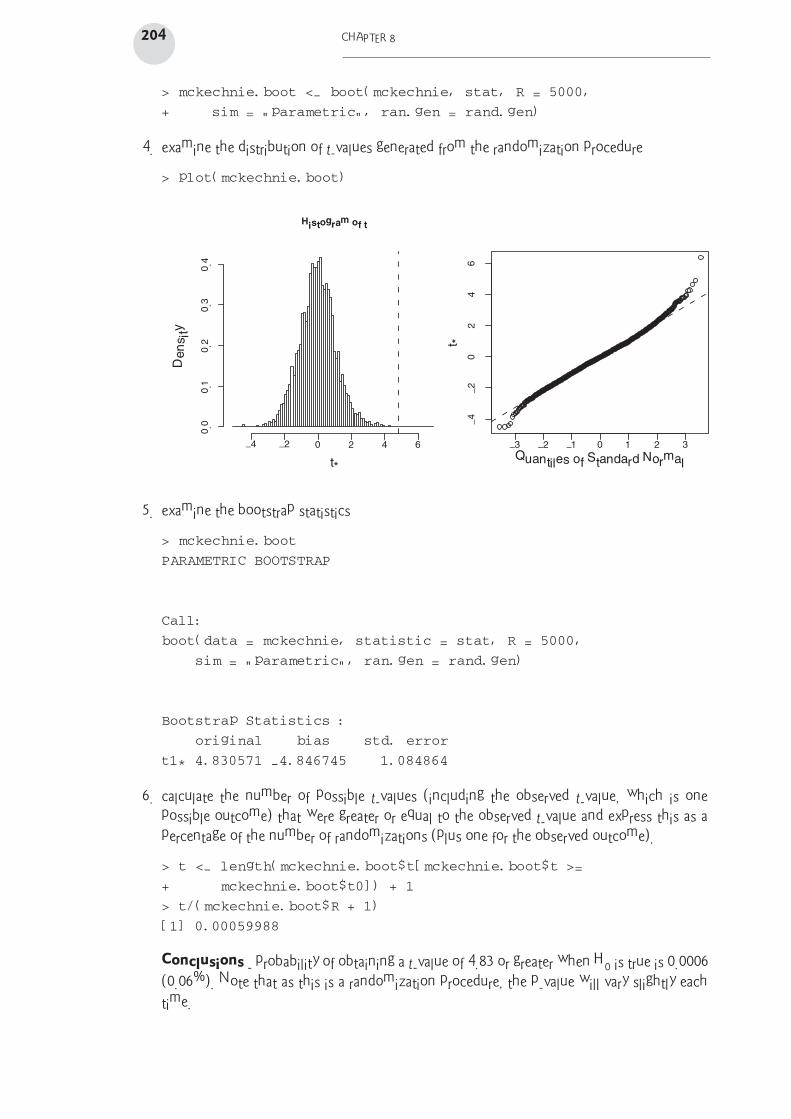
204 CHAPTER 8
> mckechnie.boot <- boot(mckechnie, stat, R = 5000,
+ sim = "parametric", ran.gen = rand.gen)
4. examine the distribution of t-values generated from the randomization procedure
> plot(mckechnie.boot)
Histogram of t
t*
De
nsity
−4 −2 0 6
0.0
0.1
0.2
0.3
0.4
−3 −2 −1 0 1 2 3
−4
−2
02
46
Quantiles of Standard Normalt*
2 4
5. examine the bootstrap statistics
> mckechnie.boot
PARAMETRIC BOOTSTRAP
Call:
boot(data = mckechnie, statistic = stat, R = 5000,
sim = "parametric", ran.gen = rand.gen)
Bootstrap Statistics :
original bias std. error
t1* 4.830571 -4.846745 1.084864
6. calculate the number of possible t-values (including the observed t-value, which is one
possible outcome) that were greater or equal to the observed t-value and express this as a
percentage of the number of randomizations (plus one for the observed outcome).
> t <- length(mckechnie.boot$t[mckechnie.boot$t >=
+ mckechnie.boot$t0]) + 1
> t/(mckechnie.boot$R + 1)
[1] 0.00059988
Conclusions - probability of obtaining a t-value of 4.83 or greater when H0 is true is 0.0006
(0.06%). Note that as this is a randomization procedure, the p-value will vary slightly each
time.
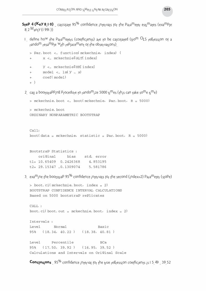
CORRELATION AND SIMPLE LINEAR REGRESSION 205
Step 4 (Key 8.10) - calculate 95% confidence intervals for the parameter estimates (example
8.2 Manly (1991))
1. define how the parameters (coefficients) are to be calculated (from OLS regression of a
random resample with replacement of the observations).
> par.boot <- function(mckechnie, index) {
+ x <- mckechnie$ALT[index]
+ y <- mckechnie$HK[index]
+ model <- lm(y ~ x)
+ coef(model)
+ }
2. call a bootstrapping procedure to randomize 5000 times (this can take some time)
> mckechnie.boot <- boot(mckechnie, par.boot, R = 5000)
> mckechnie.boot
ORDINARY NONPARAMETRIC BOOTSTRAP
Call:
boot(data = mckechnie, statistic = par.boot, R = 5000)
Bootstrap Statistics :
original bias std. error
t1* 10.65409 0.2426368 4.853195
t2* 29.15347 -0.1309074 5.581786
3. examine the bootstrap 95% confidence intervals for the second (index=2) parameter (slope)
> boot.ci(mckechnie.boot, index = 2)
BOOTSTRAP CONFIDENCE INTERVAL CALCULATIONS
Based on 5000 bootstrap replicates
CALL :
boot.ci(boot.out = mckechnie.boot, index = 2)
Intervals :
Level Normal Basic
95% (18.34, 40.22 ) (18.38, 40.81 )
Level Percentile BCa
95% (17.50, 39.92 ) (16.95, 39.52 )
Calculations and Intervals on Original Scale
Conclusions - 95% confidence interval for the true regression coefficients is 15.49 - 39.52
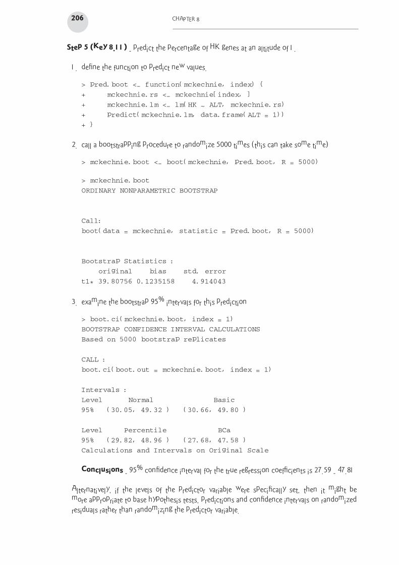
206 CHAPTER 8
Step 5 (Key 8.11) - predict the percentage of HK genes at an altitude of 1.
1. define the function to predict new values.
> pred.boot <- function(mckechnie, index) {
+ mckechnie.rs <- mckechnie[index, ]
+ mckechnie.lm <- lm(HK ~ ALT, mckechnie.rs)
+ predict(mckechnie.lm, data.frame(ALT = 1))
+ }
2. call a bootstrapping procedure to randomize 5000 times (this can take some time)
> mckechnie.boot <- boot(mckechnie, pred.boot, R = 5000)
> mckechnie.boot
ORDINARY NONPARAMETRIC BOOTSTRAP
Call:
boot(data = mckechnie, statistic = pred.boot, R = 5000)
Bootstrap Statistics :
original bias std. error
t1* 39.80756 0.1235158 4.914043
3. examine the bootstrap 95% intervals for this prediction
> boot.ci(mckechnie.boot, index = 1)
BOOTSTRAP CONFIDENCE INTERVAL CALCULATIONS
Based on 5000 bootstrap replicates
CALL :
boot.ci(boot.out = mckechnie.boot, index = 1)
Intervals :
Level Normal Basic
95% (30.05, 49.32 ) (30.66, 49.80 )
Level Percentile BCa
95% (29.82, 48.96 ) (27.68, 47.58 )
Calculations and Intervals on Original Scale
Conclusions - 95% confidence interval for the true regression coefficients is 27.59 - 47.81
Alternatively, if the levels of the predictor variable were specifically set, then it might be
more appropriate to base hypothesis tests, predictions and confidence intervals on randomized
residuals rather than randomizing the predictor variable.
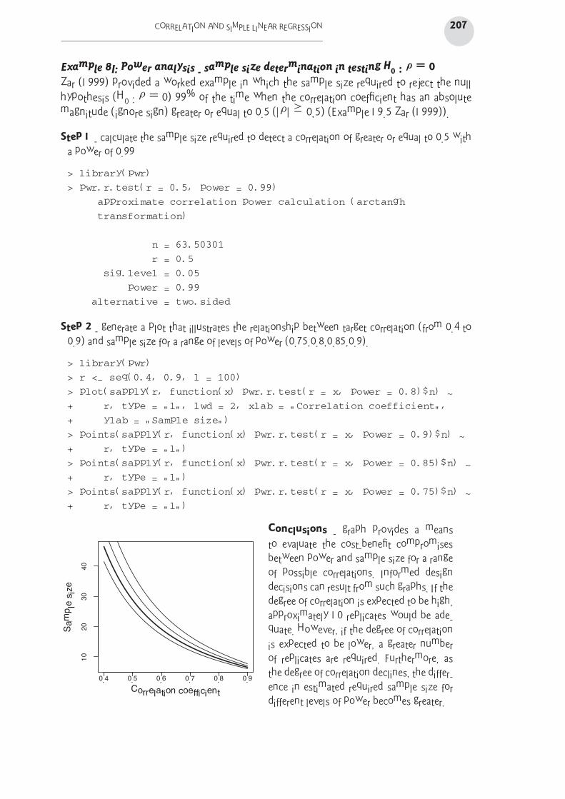
CORRELATION AND SIMPLE LINEAR REGRESSION 207
Example 8I: Power analysis - sample size determination in testing H0 : ρ = 0
Zar (1999) provided a worked example in which the sample size required to reject the null
hypothesis (H0 : ρ = 0) 99% of the time when the correlation coefficient has an absolute
magnitude (ignore sign) greater or equal to 0.5 (|ρ| ≥ 0.5) (Example 19.5 Zar (1999)).
Step 1 - calculate the sample size required to detect a correlation of greater or equal to 0.5 with
a power of 0.99
> library(pwr)
> pwr.r.test(r = 0.5, power = 0.99)
approximate correlation power calculation (arctangh
transformation)
n = 63.50301
r = 0.5
sig.level = 0.05
power = 0.99
alternative = two.sided
Step 2 - generate a plot that illustrates the relationship between target correlation (from 0.4 to
0.9) and sample size for a range of levels of power (0.75,0.8,0.85,0.9).
> library(pwr)
> r <- seq(0.4, 0.9, l = 100)
> plot(sapply(r, function(x) pwr.r.test(r = x, power = 0.8)$n) ~
+ r, type = "l", lwd = 2, xlab = "Correlation coefficient",
+ ylab = "Sample size")
> points(sapply(r, function(x) pwr.r.test(r = x, power = 0.9)$n) ~
+ r, type = "l")
> points(sapply(r, function(x) pwr.r.test(r = x, power = 0.85)$n) ~
+ r, type = "l")
> points(sapply(r, function(x) pwr.r.test(r = x, power = 0.75)$n) ~
+ r, type = "l")
0.4 0.5 0.6 0.7 0.8 0.9
10
20
30
40
Correlation coefficient
Sa
mp
le s
ize
Conclusions - graph provides a means
to evaluate the cost-benefit compromises
between power and sample size for a range
of possible correlations. Informed design
decisions can result from such graphs. If the
degree of correlation is expected to be high,
approximately 10 replicates would be ade-
quate. However, if the degree of correlation
is expected to be lower, a greater number
of replicates are required. Furthermore, as
the degree of correlation declines, the differ-
ence in estimated required sample size for
different levels of power becomes greater.