Web viewIt can be noted that the numerical value agrees with the exact one up to 7 digits, even though we use only 5 nodes for the grid span. Nevertheless, the

[100] 003 Chapter 3 Integration, Tutorial by www.msharpmath.com

[100] 003 revised on 2012.12.08 cemmath

The Simple is the Best

Chapter 3 Integration

3-1 Single Integration3-2 Integrated Function and Plot3-3 Multiple Integration3-4 Area Properties For Closed Curves in 2D3-5 Surface Integral 3-6 Line Integral 3-7 Summary of Syntax3-8 References

Integration of mathematical functions is primarily based on the Gauss quadrature, and utilizes a new Umbrella ‘int’. For users’ convenience however, well-known trapezoidal rule and Simpson’s rule are also provided by means of Spokes. In addition, the line integrals and the surface integrals are also discussed.

Section 3-1 Single Integration

■ Syntax of Umbrella ‘int’. Integration of a function with respect to a single independent variable can be written as

I=∫a

b

f ( x )dx

The syntax of our new Umbrella ‘int’ for this situation is

int .x[n=26,g=1](a,b) ( <<opt>>,f(x), g(x), h(x), … )

1


or

x = (a,b).span(n,g=1); int [x] ( <<opt>>,f(x), g(x), h(x), … )

and the relevant Spokes are

.poly(nth) Newton-Cotes integration with polynomial of degree nth<=8 .quad(num) Gauss-Legendre quadrature with number of points <=6 .togo(F) takeout an integrated function as a matrix F

.return return an integrated function as a matrix

.plot plot integrated function for one-variable case

The grid span defined in the Hub of ‘int’ implies that the given interval

a≤ x≤b is first divided into n−1 subintervals (equal spacing if g=1) and the

integral is evaluated by means of local sums

I ≅∑i=2

n

∫x i−1

x i

f ( x )dx

■ Default Case. Integration over a given subinterval x i−1≤ x≤ xi is by default performed based on the fourth-degree Gauss-Legendre quadrature, i.e. the Spoke ‘quad(5)’ is used by default if not specified explicitly.

(Example 3-1-1) Let us start with a simple example which has an exact value

∫0

1 11+x2 dx=

π4

This can be confirmed by the following commands

%> Umbrella 'int'#> int .x[5](0,1) ( 1/(1+x*x) );#> pi/4;

which result in

ans = 0.7853982ans = 0.7853982

2


It can be noted that the numerical value agrees with the exact one up to 7 digits, even though we use only 5 nodes for the grid span. Nevertheless, the total number of evaluating the given function is actually (5−1 )

× (4+1 )=20 for

this case, as can be seen later. ◀

■ Comparison with Numerical Theories. The most simplest methods of integration among the existing numerical theories would be the lower and upper summations, I L , IU, based on the zeroth-degree polynomial (i.e. constant over each subinterval)

∫a

b

f ( x )dx ≅ I L=h [ f (x1 )+ f ( x2 )+ f (x3 )+…+ f (xn−1 ) ]

∫a

b

f ( x )dx ≅ IU=h [ f (x2 )+ f ( x3 )+ f (x4 )+…+ f (xn ) ]

where h=(b−a ) / (n−1 ) and x i=a+h (i−1 ) , i=1,2,3 ,…,n.

For monotonously increasing functions, it is well known that

I L≤∫a

b

f ( x )dx≤ IU

As an example, for a special case of f ( x )=e2 x ,0≤x ≤1 and n=5, we have

I L=(1 / 4 ) [e0+e0.5+e1+e1.5 ]=2.4621730IU=(1 / 4 ) [e0.5+e1+e1.5+e2 ]=4.0594371

∫0

1

e2 xdx= 12

(e2−1 )=3.1945280

This can be also confirmed from Figure 1 where the lower-step and upper-step functions are shown together with the given function. Corresponding Cemmath commands are

3


#> .hold; plot .x (0,1) ( exp(2*x) ); plot .x[5](0,1) ( exp(2*x) ).lstep; plot .x[5](0,1) ( exp(2*x) ).ustep; plot .x[5](0,1) ( exp(2*x) ).ystem;#> plot;

Figure 1 Zeroth- degree polynomial integration

(Example 3-1-2) For practical comparison, Cemmath provides a useful Spoke ‘poly’ which represents the degree of polynomial used for integration in each subinterval.

I L=(1 / 4 ) [e0+e0.5+e1+e1.5 ]=2.4621730IU=(1 / 4 ) [e0.5+e1+e1.5+e2 ]=4.0594371

#> int .x[5](0,1) ( exp(2*x) ).poly(0);#> int .x[5](1,0) ( exp(2*x) ).poly(0);ans = 2.4621730ans = -4.0594371

In the above, it should be noted that Spoke ‘poly(0)’ always starts from the leftmost point, and thus the grid direction must be reversed to evaluate IU

corresponding to upper-step approximation of a given function. Of course from definition, the numerical results are exactly the same as the aforementioned values, where the minus sign is due to reversing grid direction. ◀

■ Trapezoidal Rule. The frequently used trapezoidal rule corresponds to the case of the first-degree polynomial approximation over each subinterval.

4


(Example 3-1-3) For the aforementioned example, numerical integration becomes (underlying numerical theories are omitted here)

∫0

1

e2 xdx≅ 12

(0.25 ) [e0+2e0.5+2e1+2 e1.5+e2 ]

¿3.2608051 (≠3.1945280 )

which can be confirmed by

#> int .x[5](0,1) ( exp(2*x) ).poly(1); ans= 3.2608051 ◀

■ Simpson’s 1/3 Rule. The Simpson’s 1/3 rule is based on the second-degree polynomial approximation over each subinterval. To apply the Simpson’s 1/3 rule, the range of integration a≤ x≤b is first divided into 2n subregions. Then, the second-degree polynomial approximation is performed over x i≤ x≤ x i+2. This is equivalent to that the interval of a≤ x≤b is divided into n subintervals and each subinterval is again divided into 2 subintervals. Therefore, the corresponding syntax for the Simpson’s 1/3 rule is

int .x[n+1,g=1](a,b) ( f(x) ) .poly(2) // 2n uniform h for g=1

Note that the Hub span is always associated with the total number of nodes not the number of subintervals.

(Example 3-1-4) For the above example, numerical integration becomes

∫0

1

e2 xdx≅ 12

(0.25 ) ¿

¿3.1956051 (≠3.1945280 )

which can be confirmed by

#> int .x[3](0,1) ( exp(2*x) ).poly(2); ans= 3.1956051

In the above, it should be noticed that the Hub span has changed from the previous case, i.e. the grid size has changed from 5 to 3. As was discussed

5


earlier, the grid size creates the number of subintervals for integration, i.e. n−1, while Spoke ‘poly’ determines how many further sub-divisions are required. ◀

■ Newton-Cotes Integration. In general, numerical methods of integration discussed above are classified as the Newton-Cotes integration. For instance, Newton-Cotes integration with the second-degree polynomial is the same as the Simpson’s 1/3 rule. The Spoke ‘poly’

.poly(nth)

performs the integration with specified degree of polynomials. Here, we employ polynomials at most up to eighth-degree. Higher degrees of polynomials are forced to become the eighth-degree internally in Cemmath.

Let us discuss what the behavior is associated with the following syntax

int .x[n=26,g=1](a,b) ( <<opt>>, f(x) ) .poly(nth)

As was mentioned so far, the Hub span distributes n nodes and thus n−1 equispaced subintervals are generated (if g=1). For each subinterval, nth-degree of polynomial is employed. This requires that each subinterval must be again divided into nth subintervals (note that both ends of each subinterval are

included at data points). Therefore, the original interval (a ,b) involves a total of (n−1 )nth subregions, where nth≤8.

■ Gauss-Legendre quadrature. Gauss-Legendre quadrature, simply called Gauss quadrature, is based on polynomials with pre-selected nodes and coefficients. In view of accuracy, Gauss quadrature is the most powerful method of integration, although error evaluation is not as simple as in the Newton-Cotes methods.

(Example 3-1-5) Consider the following case

∫−1

1

ex dx=e−1e≅ 2.35040238…

This can be solved by

6


#> int .x[2](-1,1) ( exp(x) ).quad(1); #> int .x[2](-1,1) ( exp(x) ).quad(2);#> int .x[2](-1,1) ( exp(x) ).quad(3);

which results in

ans = 2.0000000ans = 2.3426961ans = 2.3503369

These values can be confirmed by the numerical formulation of Gauss quadrature

I 0=∫−1

1

exdx ≅ 2e0=2

I 1=∫−1

1

ex dx≅ e−1 /√3+e1 /√3=2.3426961

I 2=∫−1

1

e xdx≅ 59

(e−√0.6+e√0.6 )+ 89e0=2.3503369

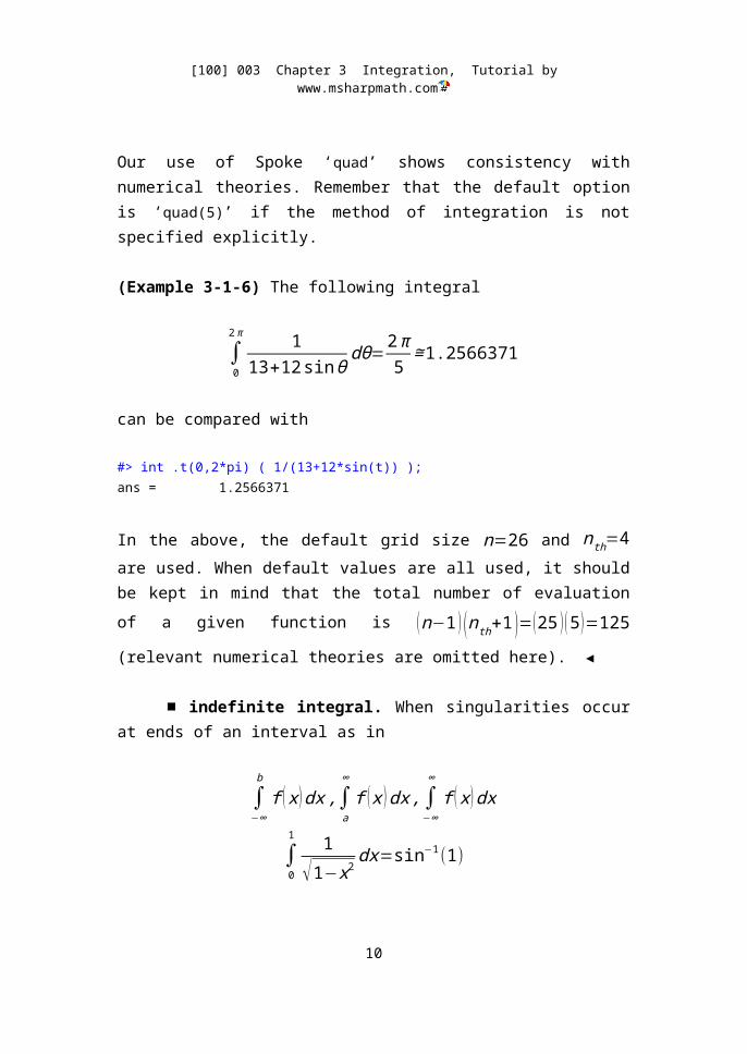
Our use of Spoke ‘quad’ shows consistency with numerical theories. Remember that the default option is ‘quad(5)’ if the method of integration is not specified explicitly.

(Example 3-1-6) The following integral

∫0

2π 113+12sin θ

dθ=2π5

≅ 1.2566371

can be compared with

#> int .t(0,2*pi) ( 1/(13+12*sin(t)) );ans = 1.2566371

In the above, the default grid size n=26 and nth=4 are used. When default values are all used, it should be kept in mind that the total number of evaluation

7


of a given function is (n−1 ) (nth+1 )=(25 ) (5 )=125 (relevant numerical theories

are omitted here). ◀

■ indefinite integral. When singularities occur at ends of an interval as in

∫−∞

b

f ( x )dx ,∫a

∞

f ( x )dx ,∫−∞

∞

f (x )dx

∫0

1 1√1−x2

dx=sin−1(1)

the given interval is splitted into small subintervals. A built-in dot function is

.integ(a,b, f(x))

Examples are

∫0

∞

e−x2

sin (x2)dx=√π4

(√2−1 )1 / 2

#> double f(x) = exp(-x^2)*sin(x^2); #> .integ(0,inf,f); // built-in dot function ans = 0.28518528

#> sqrt(pi)/4*sqrt(sqrt(2)-1);ans = 0.28518528

∫0

1 1√1−x2

dx=sin−1(1)

#> double f(x) = 1/sqrt(1-x^2); #> .integ(0,1,f); // built-in dot function ans = 1.5707658

#> asin(1); ans = 1.5707963

A user-function equivalent to the above built-in function is

//-------------------// indefinite integral//-------------------double integ(a,b, f(x)) {

8


aa = a; bb = b; flip = 1; if(a > b) { aa = b; bb = a; flip = -1; } (sum, h,r) = (0, 0.05, 1.2); if( aa < -0.5*inf && 0.5*inf < bb ) { // -inf<x<inf a = 0; for[300] { sum += int.x(a,a+h) ( f(x) ) + int.x(-a-h,-a) ( f(x) ); a += h; h *= r; } } else if( aa < -0.5*inf ) { // -inf<x<bb a = bb; for[300] { sum += int.x(a-h,a) ( f(x) ); a -= h; h *= r; } } else if( 0.5*inf < bb ) { // aa<x<inf a = aa; for[300] { sum += int.x(a,a+h) ( f(x) ); a += h; h *= r; } } else { // aa<x<bb a = b = 0.5*(aa+bb); h = 0.25*(bb-aa); for[30] { sumo = sum; sum += int.x(a,a+h) (f(x)) + int.x(b-h,b) (f(x)); a += h; b -= h; h *= 0.5; if( sum.-.sumo < 1.e-8) break; } }

return sum*flip;}

Section 3-2 Integrated Function and Plot

■ Integrated Function. The integrated function is here allowed only for a single integration which can be written as

F ( x )=∫a

x

f ( t )dt

Note that F (a )=0 by definition. The syntax for this integrated function is using Spoke ‘togo’ or ‘return’

int .x[n=26,g=1](a,b) ( <<opt>>, f(x), g(x), … ) .togo(F,G, …);int .x[n=26,g=1](a,b) ( <<opt>>, f(x), g(x), … ) .return;

9


where F is a matrix the size of which is exactly the same as the grid span. Meanwhile, Spoke ‘return’ does not require a variable, and returns the integration result as a matrix. However, for double and triple integration, use of Spokes ‘togo’ and ‘return’ is invalid.

An example of using Spokes ‘togo’ and ‘return’ is as follows.

#> int .x[5](0,1) ( x, x*x ) .togo (P,Q); P; Q; #> int .x[5](0,1) ( x, x*x ) .return;

The results show the value of integration and 5×1 matrix P and Q, as well as

5×2 matrix.

ans =[ 0.5 0.33333 ]

P = [ 0 ] [ 0.03125 ] [ 0.125 ] [ 0.28125 ] [ 0.5 ] Q = [ 0 ] [ 0.0052083 ] [ 0.041667 ] [ 0.14062 ] [ 0.33333 ] ans = [ 0 0 ] [ 0.03125 0.0052083 ] [ 0.125 0.041667 ] [ 0.28125 0.14062 ] [ 0.5 0.33333 ]

■ Plot of Integrated Function. The integrated function can be also drawn by using Spoke ‘plot’ or ‘plot+’. Let us consider the integrals

Sn ( x )=∫0

x

sin (t n )dt ,Cn ( x )=∫0

x

cos (t n )dt

10


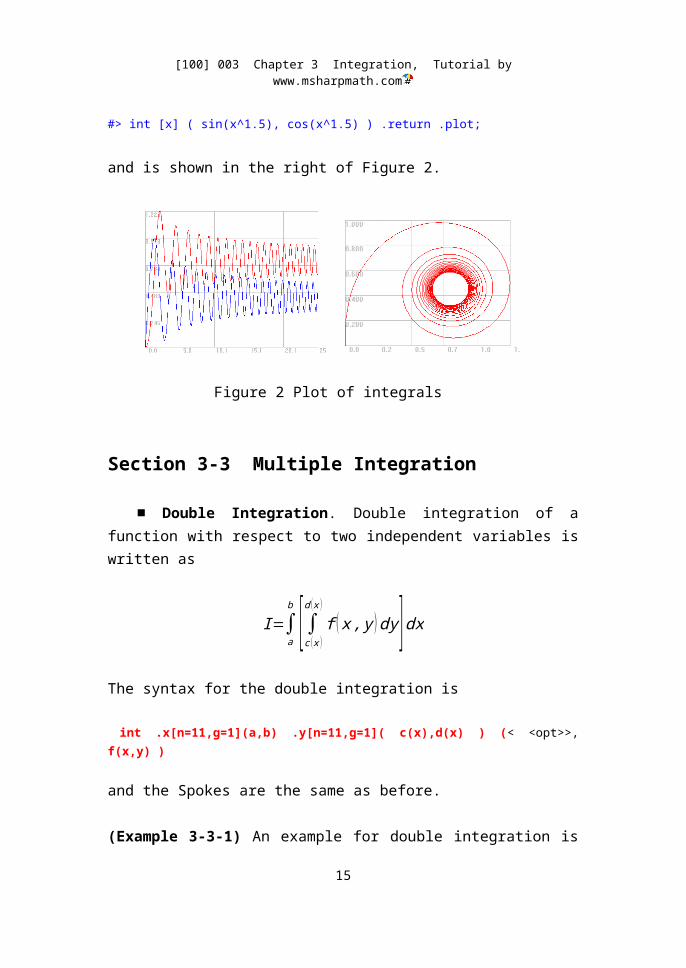
where the case of n=2 corresponds to the well-known Fresnel integrals. An example is

#> x = (0,8*pi).span(1001);; #> int[x] ( sin(x^1.5), cos(x^1.5) ) .plot;

In the above, the grid span for x–coordinate is generated by the Tuple discussed earlier. The results of integrals are shown in the left of Figure 2. An interesting result is the Sn ( x ) versus Cn ( x ) plot which can be found by the following commands,

#> x = (0,8*pi).span(1001);;#> int [x] ( sin(x^1.5), cos(x^1.5) ) .togo(S,C);;#> plot(S,C);

or equivalently

#> int [x] ( sin(x^1.5), cos(x^1.5) ) .return .plot;

and is shown in the right of Figure 2.

Figure 2 Plot of integrals

Section 3-3 Multiple Integration

■ Double Integration. Double integration of a function with respect to two independent variables is written as

11


I=∫a

b [∫c ( x )

d ( x )

f ( x , y ) dy ]dxThe syntax for the double integration is

int .x[n=11,g=1](a,b) .y[n=11,g=1]( c(x),d(x) ) (< <opt>>, f(x,y) )

and the Spokes are the same as before.

(Example 3-3-1) An example for double integration is taken from ref. [1]

I=∫0

1

∫−√ x− x2

√x−x2

(x−x2− y2)dydx= π32

which can be solved by

#> int .x[11](0,1) .y[11]( -sqrt(x-x*x),sqrt(x-x*x) ) (x-x*x-y*y );#> pi/32;ans = 0.0981746ans = 0.0981748

Numerical result agrees with the exact value up to 5 digits. Since we employed the fourth-degree Gauss quadrature, the equivalent grid size is (5 ⋅10 )× (5 ⋅10 )=50×50. However, the degree of agreement deteriorates when the typical trapezoidal rule is applied by Spoke ‘poly’ as follows

#> int .x[51](0,1) .y[51]( -sqrt(x-x*x),sqrt(x-x*x) ) (x-x*x-y*y ).poly(1);

ans = 0.0981316

Note that, even though an equivalent grid size of is of similar order in grid resolution, the trapezoidal rule is inferior to the Gauss quadrature from the standpoint of accuracy. ◀

■ Triple Integration. Triple integration of a function with respect to three independent variables

12

50 50


I=∫a

b [∫c ( x )

d ( x ) { ∫u ( x , y )

v (x , y )

f ( x , y , z ) dz}dy ]dxcan be treated by the following syntax

int .x[n=6,g=1](a,b) .y[n=6,g=1](c(x),d(x)) .z[n=6,g=1] (u(x,y),v(x,y)) ( <<opt>>, f(x,y,z) )

Also, the same Spokes for ‘int’ are applicable to this case.

(Example 3-3-2) An example for triple integration is also taken from ref. [1]

I=∫0

3

∫1

x

∫z−x

z+x

[e2x (2 y−z ) ]dz dy dx=18+ 59e6

8

which is solved by

#> int .x(0,3) .z(1,x) .y(z-x,z+x) ( exp(2*x)*(2*y-z) );#> 1/8+ 59*exp(6)/8;ans = 2975.4123518ans = 2975.4123520

where the default size 6×6×6 is employed. Numerical result agrees with the

exact value up to 9 digits. Nevertheless, the trapezoidal rule yields

#> int .x[26](0,3) .z[26](1,x) .y[26](z-x,z+x) ( exp(2*x)*(2*y-z) ).poly(1);

ans = 3011.1664032

where an equivalent grid size of 25×25×25 with a trapezoidal rule is equivalent to that of (5 ⋅5 )× (5 ⋅5 )× (5 ⋅5 )=25×25×25 with the fourth-degree Gauss quadrature. ◀

Section 3-4 Area Properties For Closed Curves in 2D

13


■ Closed Curves in 2D. In mathematics, it is well known that the area enclosed by a closed curve C

in the xy-plane can be found from

A≡∫AdA=∮

C

12(xdy− ydx )

Similarly, several well-known area properties such as the moment can be also determined by integration along the curve. Among those are

Ax≡∫AxdA A y ≡∫

AydA

Axx≡∫Ax2dA A xy≡∫

AxydA A yy≡∫

Ay2dA

where the boundary of A must be a closed curve C.

These area properties for closed curves can be obtained by using Umbrella ‘plot’ and its Spokes listed below.

.int1da(a) area enclosed by a closed curve.intxda(ax) area properties

.intyda(ay) .intxxda(axx) .intxyda(axy)

.intyyda(ayy)

Here, we use the lower-case ‘a’ instead of the upper-case ‘A’, since ‘intdA’ shall be used for the case of vector area element. Note that the Spoke for evaluating the enclosed area is ‘int1da’ not ‘intda’. This is because that Spoke ‘intda’ shall be used in the surface integral. The meaning of each Spoke listed above is straightforward from its name. One thing to note is that the closed curve should be defined in a counterclockwise sense for correct sign (sometimes, it doesn’t matter whether the sign is plus or minus).

(Example 3-4-1) Consider a closed curve enclosed by two curves y=4−x2 and y=0. We want to evaluate

14


∫AdA=32

3,∫Ay2dA=4096

105

The following Cemmath commands

#> .hold; plot .line(-2,0, 2,0); plot .x(2,-2) ( 4-x*x ) .link .int1da(area) .intyyda(ayy); plot .line(0,-1, 0,4);#> plot;#> area / (32/3) ;#> ayy / ( 4096/105 );

displays a closed curve (shown in Figure 3) and returns two values ‘area’ and ‘ayy’. For convenience, numerical values are compared with the exact values in a ratio form. For example,

area / (32/3) = 0.9996001ayy / ( 4096/105 ) = 0.9990671

Figure 3 Area properties for a closed curve

For this special case, numerical values show agreement with exact values to a degree of accuracy up to only 3 digits (even with default grid size of 51). It is apparent that Gauss quadrature would yield numerical values of much higher accuracy, of course. However under certain conditions, the integration becomes extremely complicated due to difficulty in expressing the closed curve. For example, the closed curve may be rotated around the z-axis. ◀

15


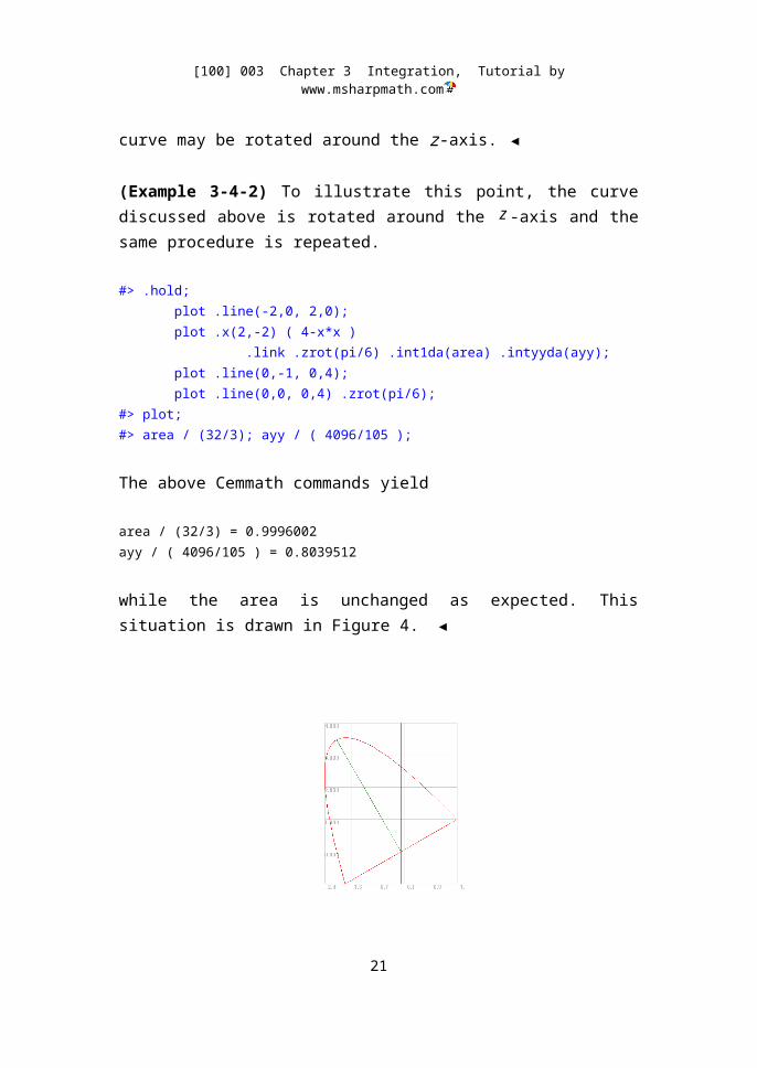
(Example 3-4-2) To illustrate this point, the curve discussed above is rotated around the -axis and the same procedure is repeated.

#> .hold; plot .line(-2,0, 2,0); plot .x(2,-2) ( 4-x*x ) .link .zrot(pi/6) .int1da(area) .intyyda(ayy); plot .line(0,-1, 0,4); plot .line(0,0, 0,4) .zrot(pi/6);#> plot;#> area / (32/3); ayy / ( 4096/105 );

The above Cemmath commands yield

area / (32/3) = 0.9996002ayy / ( 4096/105 ) = 0.8039512

while the area is unchanged as expected. This situation is drawn in Figure 4. ◀

Figure 4 Area property for a rotated closed curve

Section 3-5 Surface Integral

■ Surface Integral (scalar case). When a surface is represented by means of parameterization, the scalar area element may be written as

16

z


dA=¿ du×d v∨¿

where d u and d v

are infinitesimal tangent vectors (details are omitted here).

Then, the surface integral is defined

∫AdAϕ (x , y , z)

where ϕ (x , y , z ) is a scalar function with respect to three spatial coordinates.

For surface integrals, we use very simple summation

∫AdAϕ (x , y , z)≅∑

idA iϕi

the accuracy of which cannot compete with well-devised formula for integration though.

To evaluate the surface integral, we use Umbrella ‘plot’ to create a surface and then employ Spoke ‘intda’

.area (a) .intda (f(x,y,z), …) (fscalar,…)

Without any loss of generality, those independent variables in the above expression are fixed to be ‘x,y,z’ since use of other variables is not of major interest.

(Example 3-5-1) Let us consider again the surface enclosed by two curves y=4−x2 and y=0. For the surface shown in Figure 5,

17


Figure 5 A filled surface for surface integral

we want to evaluate the following surface integrals

∫AdA ,∫

AxdA ,∫

AydA ,∫

Ax2dA ,∫

AxydA ,∫

Ay2dA ,∫

Ax2(1+0.1 xy)dA

Our attempt to treat this problem begins with creating a filled surface and then uses Spoke ‘intda’

#> plot .x[51](-2,2) ( 0, 4-x*x ) .fill[51] .area(a) .intda ( x, y, x*x, x*y, y*y, x*x*(1+0.1*(x*y)) ) ( ax, ay, axx, axy, ayy, rhoaxx ); #> a; ax; ay; axx; axy; ayy; rhoaxx;

which results in

a = 10.6624000ax = 0.0000000ay = 17.0496039axx = 8.5333320axy = 0.0000000ayy = 38.9510297rhoaxx = 8.5333320

In particular, a comment is placed on the value of ‘ayy’. The value obtained in terms of close-curve integration was 38.9731331, which is somehow different from the value obtained through surface integral. The reason for the occurrence of this slight difference lies in the procedure of integration, as was mentioned

18


earlier. ◀

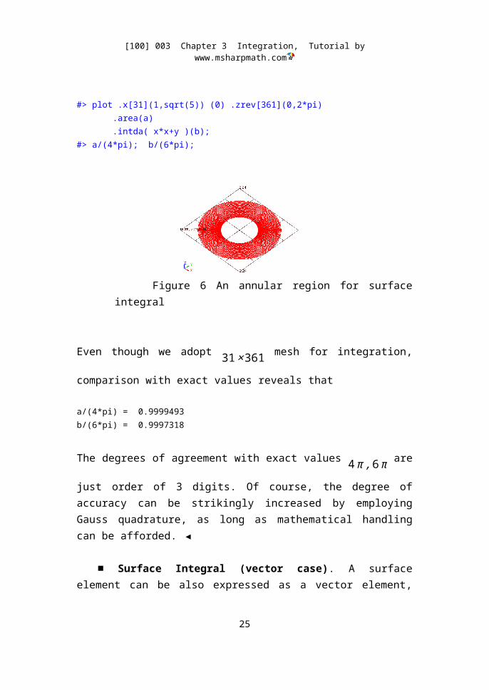
(Example 3-5-2) The next example considers a surface enclosed by an annulus shown in Figure 6. The annular region is created first and then the desired surface integral is performed by

#> plot .x[31](1,sqrt(5)) (0) .zrev[361](0,2*pi) .area(a) .intda( x*x+y )(b);#> a/(4*pi); b/(6*pi);

Figure 6 An annular region for surface integral

Even though we adopt 31×361 mesh for integration, comparison with exact

values reveals that

a/(4*pi) = 0.9999493b/(6*pi) = 0.9997318

The degrees of agreement with exact values 4 π ,6 π are just order of 3 digits.

Of course, the degree of accuracy can be strikingly increased by employing Gauss quadrature, as long as mathematical handling can be afforded. ◀

■ Surface Integral (vector case). A surface element can be also expressed as a vector element, and thus the surface integral can be presented in several different ways, e.g.

19


∫Ad A⃗ ⋅ F⃗ (x , y , z )

∫Ad A⃗× F⃗ (x , y , z)

∫Ad A⃗ ϕ (x , y , z)

where the surface element d A⃗=du×d v is normally defined from the right-hand rule. In addition, since d A⃗=i dydz+ j dzdx+k dxdy , it can be noted that

∫Ad A⃗ ⋅ F⃗=∫

AP(x , y , z)dydz+Q(x , y , z)dzdx+R(x , y , z)dxdy

where F⃗=(P ,Q ,R). This can be used to confirm the following equality

V=13∫A

xdydz+ ydzdx+zdxdy

for a closed surface A, where V designates the volume enclosed by the closed surface.

Integration with infinitesimal vector elements can be performed by applying the Spokes listed below.

.intdA * (Fx(x,y,z),Fy(x,y,z),Fz(x,y,z)) (fscalar) .intdA ^ (Fx(x,y,z),Fy(x,y,z),Fz(x,y,z)) (Fmatrix) .intdA (f(x,y,z)) (Fmatrix)

Note that the spatial coordinates are always ‘x,y,z’ regardless of the Hub variables in generating surface.

(Example 3-5-3) Consider a sphere of radius 1 and evaluate

20


∫Ad A⃗ ⋅ F⃗=∫

Ad A⃗ ⋅(x ,2 y ,3 z )=∫

VdV ∇⋅ (x ,2 y ,3 z )=6V

where the Gauss’s divergence theorem is applied to convert from surface to volume integral. This is solved by

#> plot .sphere[101,101](1) .intdA*(x,2*y,3*z)(fs);#> fs/(8*pi);

which results in

ans = 0.99911617

Comparison with the exact value shows about 0.1% error. ◀

(Example 3-5-4) For a sphere of radius 1, V= 13∫A

xdydz+ ydzdx +zdxdy can

be easily confirmed by

#> plot .sphere[101,101](1) .intdA*(x,y,z)(fs);#> fs/(4*pi)

which results in

ans = 0.9990956 ◀

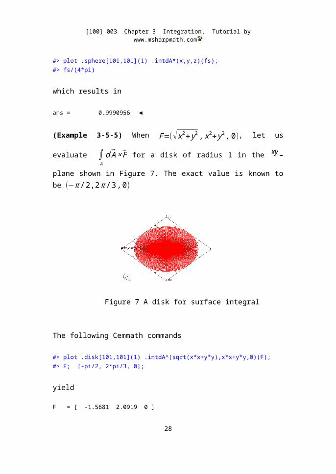
(Example 3-5-5) When F=(√x2+ y2 , x2+ y2,0), let us evaluate ∫Ad A⃗× F⃗

for a disk of radius 1 in the –plane shown in Figure 7. The exact value is known to be (−π /2,2 π / 3 ,0)

21

xy


Figure 7 A disk for surface integral

The following Cemmath commands

#> plot .disk[101,101](1) .intdA^(sqrt(x*x+y*y),x*x+y*y,0)(F);#> F; [-pi/2, 2*pi/3, 0];

yield

F = [ -1.5681 2.0919 0 ] ans = [ -1.5708 2.0944 0 ] ◀

(Example 3-5-6) Evaluate ∫Azd A⃗ for a sphere of radius 1 located at the origin.

The exact value is (0,0,4 π / 3). We solve this problem by

#> plot .sphere[101,101](1) .intdA (z)(F);#> F; [0,0, 4*pi/3];

The results are

F = [ 2.61564e-018 3.32503e-018 4.18535 ]ans = [ 0 0 4.18879 ] ◀

■ Surface Integral for Closed Surface. A finite volume in 3D can be defined by a certain closed surface the inside of which is defined as the inner region of the volume. For closed surfaces, one of the most interesting surface integrals would be the Archimedes principle combined with the Gauss’s divergence theorem, i.e.

22


∫Ad A⃗ ( ρgz )=∫

VdV ∇ (ρgz )= ρg k⃗∫

VdV=k⃗ ( ρgV )

From this principle, it is possible to evaluate the volume enclosed by a closed surface. However, the use of Spoke ‘volume’ is something like DIY (do it yourself). In other words, Cemmath never guarantee whether the geometry of interest is a closed surface or not.

(Example 3-5-7) Consider a torus generated by revolving a circle defined as

(x−12 )

2

+z2=( 12 )

2

around the z–axis. Its surface area and volume are known to be

A=π 2 ,V=14π2. Let us solve this problem by

#> plot .torus[51,51](0.5,0.5) .area(a) .volume(v); #> a/(pi*pi); v/(0.25*pi*pi);ans = 0.9976997ans = 0.9947454

where the torus is shown in Figure 8. As a matter of fact, the Spoke ‘volume’ has been originated from Spoke ‘.intdA (0,0,z)’ the reason of which is already discussed above. ◀

Figure 8 A torus for surface integral

23


(Example 3-5-8) A frustum with square base can be drawn by Spoke ‘frustum’, e.g.

#> plot .frustum[51,5,51](3,2,2) .area(a) .volume(v); #> a/56; v/(76/3);

the result of which is shown in Figure 9.

Figure 9 A frustum with square base

We can easily calculate the surface area and the volume of a frustum with square base

A=2¿

where the exact value is A=56 ,V=76/3. The numerical results show that

a/56 = 1.0000000v/(76/3) = 1.0000105

Agreement is fairly good because all the surfaces are flat. ◀

Section 3-6 Line Integral

■ Line Integral (vector case). The line integral along a curve C is defined

as

24


∫Cd L⃗ ⋅ F⃗=∫

CP ( x , y , z )dx+Q ( x , y , z )dy+R ( x , y , z )dz

∫Cd L⃗× F⃗

∫Cd L⃗ ϕ ( x , y , z )

where F⃗=i P(x , y , z )+ j Q(x , y , z )+k R(x , y , z) and d L⃗=i dx+ j dy+k dz.

The line integrals with vector line element are treated by Spoke ‘ intdL’. A limitation for the line integral is that the curve C must be defined as 3D curve.

The corresponding syntax for Spoke ‘intdL’ is

.intdL * (Fx(x,y,z),Fy(x,y,z),Fz(x,y,z)) (fscalar).intdL ^ (Fx(x,y,z),Fy(x,y,z),Fz(x,y,z)) (Fmatrix).intdL (f(x,y,z),…) (Fmatrix,…)

where the vector field is F=(Fx,Fy,Fz), and the results are saved on the scalar

fscalar or the matrix Fmatrix. Note that a special case is ∫Cd L⃗ (1 )=L⃗f−L⃗i.

(Example 3-6-1) Consider a curve C defined as x2

32 + y2

22 =1. It can be then

shown that

∫C

− ydx+xdyx2+ y2 =2π

Even though the curve C lies in the xy–plane, we have to solve this problem in

3D space as shown in Figure 10. The corresponding Cemmath commands and the results are

#> plot .@t[101](0,2*pi) ( 3*cos(t),2*sin(t),0 ) .intdL*( -y/(x*x+y*y), x/(x*x+y*y) )(fval);#> fval/(2*pi)ans = 1.0003291 ◀

25


Figure 10 An ellipse in the -plane for line integral

(Example 3-6-2) Consider a helix C defined by ( x , y , z )=¿ where π ≤θ≤3π .

Let us confirm the following line integral

∫Cydx+xdy+zdz=π2

from the following commands

#> plot .@t(pi,3*pi) ( cos(t),sin(t),0.5*t ) .intdL*(y,x,z) (fval);#> fval/(pi*pi) ans = 0.9999998

The corresponding curve is shown in Figure 11. ◀

26

xy


Figure 11 A helix for line integral

(Example 3-6-3) For a helix C shown in Figure 11, let us confirm

∫Cd L⃗× ( y , x , z )=π j and ∫

Cd L⃗ (1 )=π k

by the following commands

#> plot .@t(pi,3*pi) ( cos(t),sin(t),0.5*t ) .intdL^(y,x,z) (Fcrs);#> plot .@t(pi,3*pi) ( cos(t),sin(t),0.5*t ) .intdL (1) (Fvec);#> Fcrs; Fvec;

The results are as follows.

Fcrs = [ 7.7212e-008 3.1416 2.0817e-017 ] Fvec = [ 0 2.498e-016 3.1416 ]

Comparison with the exact solutions shows good agreements. ◀

■ Line Integral (scalar case). Another type of line integral along a curve C with scalar line element can be defined as

∫CdLϕ(x , y , z )≡∫

C¿d L⃗∨ϕ (x , y , z )

27


where ϕ (x , y , z ) is a scalar function. Such a line integral is treated by Spoke ‘intdl’. The syntax for the Spoke ‘intdl’ is

.intdl( f(x,y,z,L), … )(fscalar, …)

where L denotes the arc length measured from the starting point.For example, the arc length can be found by ‘.intdl(1)(arclen)’. Note that the lower-cased ‘dl’ denotes a scalar line element, whereas the upper-cased ‘dL’ denotes a vector line element.

(Example 3-6-4) We can find the arc length of the helix considered in (example 3-6-2) and a line integral

∫CdL (L )=1

2 [ L (3π ) ]2=5 π2

2, since L ( t )=√5

2(t−π )

by the following commands

#> plot .@t[101](pi,3*pi) ( cos(t),sin(t),0.5*t ) .intdl(1, L) (arclen, f); #> arclen/(sqrt(5)*pi);#> f/(2.5*pi*pi);

where the results are

ans = 0.9998684ans = 1.0097342

Note that a fairly large number of segments are required to get 3 digits accuracy. ◀

Section 3-7 Summary of Syntax

■ Single and Multiple Integration. The syntax of single and multiple integration is

int .x[n=26,g=1](a,b) ( <<opt>>, f(x),g(x),h(x), … ) int .x[n=11,g=1](a,b) .y[n=11,g=1](c(x),d(x)) ( <<opt>>, f(x,y) ) int .x[n=6,g=1](a,b)

28


.y[n=6,g=1](c(x),d(x))

.z[n=6,g=1] (u(x,y),v(x,y)) ( <<opt>>, f(x,y,z) )

■ Spokes. The Spokes for Umbrella ‘int’ are

.poly(nth) Newton-Cotes integration with polynomial of nth<=8 .quad(num) Gauss-Legendre quadrature with number of points num<=6.togo(F) takeout an integrated function as a matrix F.return return an integrated function as a matrix.plot plot an integrated function for one-variable case

■ Spokes for ‘plot’. The line and surface integrals associated with geometries are found by using Umbrella ‘plot’ and its relevant Spokes as

.int1da(a) area enclosed by a closed curve

.intxda(ax) area properties .intyda(ay) .intxxda(axx) .intxyda(axy)

.intyyda(ayy) .area (a).volume(v) // for closed surface only

.intda ( f(x,y,z), … ) (fscalar, …).intdl ( f(x,y,z,L), … ) (fscalar, …)

where L is an arc length measured from the starting point

.intdA * (Fx(x,y,z),Fy(x,y,z),Fz(x,y,z)) (fscalar) .intdA ^ (Fx(x,y,z),Fy(x,y,z),Fz(x,y,z)) (Fmatrix).intdA (f(x,y,z)) (Fmatrix)

.intdL * (Fx(x,y,z),Fy(x,y,z),Fz(x,y,z)) (fscalar)

.intdL ^ (Fx(x,y,z),Fy(x,y,z),Fz(x,y,z)) (Fmatrix)

.intdL (f(x,y,z),…) (Fmatrix,…)

Section 3-8 References

[1] R.E. Larson, R.P. Hostetler, B.H. Edwards, Calculus with Analytic Geometry, 6ed., Houghton Mifflin Co., (1998)

29


[2] H.B. Wilson, L.H. Turcotte, Advanced Mathematics and Mechanics Applications Using MATLAB, 2ed., CRC Press (1997).

30

Documents

Web viewIt can be noted that the numerical value agrees with the exact one up to 7 digits, even though we use only 5 nodes for the grid span. Nevertheless, the