Embed Size (px)
Citation preview

Wealth Gradients in Early Childhood Cognitive Development in Five Latin American Countries
Norbert Schady, Jere Behrman, Maria Caridad Araujo, Rodrigo Azuero, Raquel Bernal, David Bravo, Florencia Lopez-Boo, Karen Macours, Daniela Marshall, Christina Paxson, and Renos Vakis
Social Sector
IDB-WP-482IDB WORKING PAPER SERIES No.
Inter-American Development Bank
January 2014
Wealth Gradients in Early Childhood Cognitive Development in Five Latin
American Countries
Norbert Schady, Jere Behrman, Maria Caridad Araujo, Rodrigo Azuero, Raquel Bernal, David Bravo,
Florencia Lopez-Boo, Karen Macours, Daniela Marshall, Christina Paxson, and Renos Vakis
2014
Inter-American Development Bank

http://www.iadb.org The opinions expressed in this publication are those of the authors and do not necessarily reflect the views of the Inter-American Development Bank, its Board of Directors, or the countries they represent.
The unauthorized commercial use of Bank documents is prohibited and may be punishable under the
Bank's policies and/or applicable laws.
Copyright © Inter-American Development Bank. This working paper may be reproduced for any non-commercial purpose. It may also be reproduced in any academic journal indexed by the American Economic Association's EconLit, with previous consent by the Inter-American Development Bank (IDB), provided that the IDB is credited and that the author(s) receive no income from the publication.
Cataloging-in-Publication data provided by the Inter-American Development Bank Felipe Herrera Library Wealth gradients in early childhood cognitive development in five Latin American countries / Norbert Schady, Jere Behrman, Maria Caridad Araujo, Rodrigo Azuero, Raquel Bernal, David Bravo, Florencia Lopez-Boo, Karen Macours, Daniela Marshall, Christina Paxson, and Renos Vakis. p. cm. — (IDB Working Paper Series ; 482) Includes bibliographical references. 1. Early childhood education —Latin America. 2. Child development—Research—Latin America. 3. Social status—Latin America. 4. Child development—Testing. I. Schady, Norbert. II. Behrman, Jere. III. Araujo, Maria Caridad. IV. Azuero, Rodrigo. V. Bernal, Raquel. VI. Bravo, David. VII. Lopez-Boo, Florencia. VIII. Macours, Karen. IX. Marshall, Daniela. X. Paxson, Christina. XI. Vakis, Renos. XII. Inter-American Development Bank. Social Sector. XIII. Series.
2014

Abstract0F
*
Research from the United States shows that gaps in early cognitive and non-cognitive ability appear early in the life cycle. Little is known about this important question for developing countries. This paper provides new evidence of sharp differences in cognitive development by socioeconomic status in early childhood for five Latin American countries. To help with comparability, we use the same measure of receptive language ability for all five countries. We find important differences in development in early childhood across countries, and steep socioeconomic gradients within every country. For the three countries where we can follow children over time, there are few substantive changes in scores once children enter school. Our results are robust to different ways of defining socioeconomic status, to different ways of standardizing outcomes, and to selective non-response on our measure of cognitive development.
JEL Classification: I24, I25
Keywords: cognitive development, poverty, gradients
* Acknowledgments: This research was supported by the Inter-American Development Bank, the World Bank, the Eunice Shriver Kennedy National Institute of Child Health and Development (Grant R01-HD065436) and Grand Challenges Canada (Grant 10036540).

1
1. Introduction Development in early childhood is an important predictor of success in adulthood in a number of
domains. Research from multiple disciplines makes clear that outcomes in early childhood are
malleable, although the window of opportunity may be short, especially for cognitive outcomes
and nutritional status. There is also evidence from developed and developing countries that
investments in early childhood can positively affect long-term trajectories (Almond and Currie
2011, and Cunha et al. 2006 are reviews for the United States; Engle et al. 2007, 2011 and
Behrman et al. 2013 are reviews for developing countries that focus primarily on the medical
literature).
This paper provides new evidence of sharp differences in cognitive development by
socioeconomic status in early childhood for five Latin American countries. It complements
research from the United States that shows that gaps in early cognitive and non-cognitive ability
appear early in the life cycle. At age 3, the difference in cognitive scores between children of
college graduates and high school dropouts in the United States is almost 1.5 standard deviations,
and this difference is stable until (at least) 18 years of age (Heckman 2008). At age 5, children in
the lowest income quartile have scores that are approximately 0.8 standard deviations lower than
those in the highest income quartile on a math test (Cunha and Heckman 2007). Duncan and
Magnuson (2013) report that average achievement gaps in math and reading between children in
the top and bottom income quintiles are more than a full standard deviation at the beginning of
kindergarten.
By and large, comparable evidence does not exist for developing countries. We are aware
of only a handful of earlier studies that seek to measure socioeconomic differences in early
childhood in developing countries. A study of poor children in rural Ecuador uses panel data to
show that there are substantial differences in cognitive development at young ages, including in
vocabulary, memory and visual integration, between children of higher and lower socioeconomic
status. The socioeconomic gradients in vocabulary (but not in other measures of cognitive
development) appear to increase between 3 and 5 years of age (Schady 2011, which builds on
Paxson and Schady 2007). Two other studies use single cross-sections of data from low-income
countries, specifically Madagascar (Fernald et al. 2011) and Cambodia and Mozambique
(Naudeau et al. 2011). These studies also find substantial differences in cognitive development

2
at young ages, with increasing gaps in the cross sections between 3 and 5/6 years of age for
some, but not all, indicators of cognitive development.
Our paper substantially extends earlier work on the subject. We highlight three important
contributions. First, we present results that are comparable for five countries, based on a
common outcome measure, child performance on the Test de Vocabulario en Imágenes Peabody
(TVIP). In all five countries, we observe socioeconomic gradients in cognitive development
(albeit of different magnitudes), which suggests that this pattern is not idiosyncratic, country-
specific, or a result of data mining. Moreover, in the rural areas of all five countries, and in the
urban areas of Chile and Colombia the distribution of socioeconomic status in the surveys we use
is broadly similar to the distribution of socioeconomic status in nationally-representative
household surveys, further suggesting that the results we report have external validity, at least in
rural areas. 1 Second, we show that our findings are robust to different ways of defining
socioeconomic status, to different ways of standardizing outcomes, and to selective non-response
on our measure of cognitive development. Finally, in three countries (Ecuador, Nicaragua, and
Peru) we exploit the longitudinal structure of the data to analyze how deficits in receptive
language ability observed at young ages evolve as children enter the early school years.
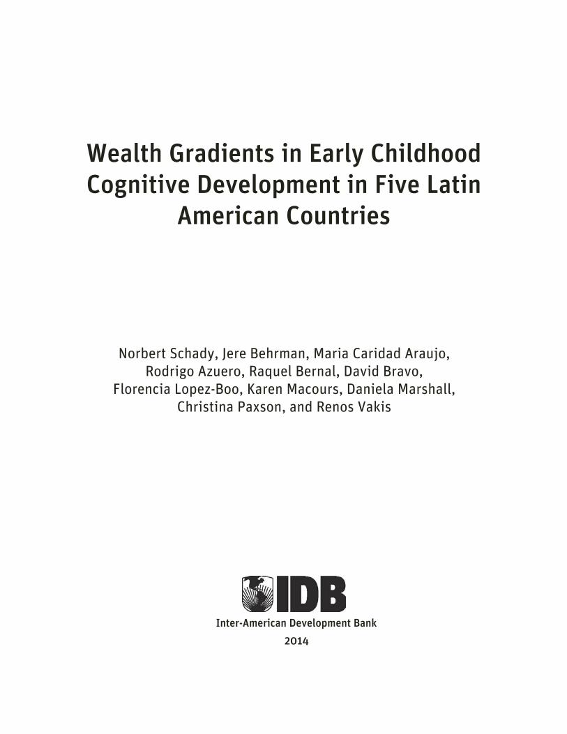
2. Data and setting We begin by describing the surveys that we use for our analysis in Table 1. The table shows that
the surveys we use vary in sample sizes and coverage. The largest samples are found in the
survey for Chile (approximately 5,400 children) and the smallest in Nicaragua and Peru (between
1,800 and 1,900 children each). The Nicaraguan survey only sampled children in rural areas,
while the data for Chile, Colombia, Ecuador and Peru covered both urban and rural areas. The
age range of children in the surveys also varies. The test of child cognitive development we use,
discussed in more detail below, is designed to be applied to children 30 months and older, and in
most of our analysis we limit the sample to children ages 36-71 months of age. In practice,
1 To make this comparison, we use nationally-representative household surveys in each of the five countries, restrict the list of assets and dwelling characteristics to those that are common to both the nationally-representative survey and the survey that was the basis for our analysis of the TVIP scores, and calculate wealth indices in the nationally-representative surveys, separately for urban and rural areas. We then re-calculate a wealth index in the surveys that we use to analyze the TVIP scores, giving each of the assets and dwelling characteristics the same weight that they receive in the calculation of the first principal component in the nationally-representative survey. Finally, we graph kernel densities of the distribution of wealth in both surveys (See Online Appendix Figure 1).

3
however, the oldest children in Chile are 57 months of age, while the youngest children in Peru
are 53 months of age.
Table 1 also shows that in three of the countries we analyze, Ecuador, Nicaragua, and
Peru, there is a panel component in the data. In Peru, there are two waves of this panel, separated
by approximately three years; in Nicaragua, there are three rounds of data collected over a four-
year period; in Ecuador, finally, there are four rounds of data collected over a seven-year period.
A major strength of our study is the use of a common measure of child cognitive
development: performance on the widely-used Test de Vocabulario en Imágenes Peabody
(TVIP), the Spanish version of the Peabody Picture Vocabulary Test (PPVT) (Dunn et al. 1986).
Children are shown slides, each of which has four pictures, and are asked to identify the picture
that corresponds to the object (for example, “boat”) or action (for example, “to measure”) named
by the test administrator. The test continues until the child has made six mistakes in the last eight
slides. The test is a measure of receptive vocabulary because children do not have to name the
objects themselves and because children need not be able to read or write. Performance on the
PPVT and TVIP at early ages has been shown to be predictive of important outcomes in a variety
of settings.2
To analyze socioeconomic gradients in TVIP scores, we construct country-specific, age-
specific z-scores by subtracting the month-of-age-specific mean of the raw score and dividing by
the month-of-age-specific standard deviation, separately by country and by urban-rural place of
residence (as in Cunha and Heckman 2007 and many others).3 As a robustness test, we also
report results that use the tables given by the test developers to standardize the test (as done by
Paxson and Schady 2007).
A fraction of children in every survey, ranging from 2 percent in Colombia to 18 percent
in Nicaragua, did not take the TVIP. Although we do not have data that are comparable across all
2 Some examples include Schady (2011), who shows that children with low levels of TVIP scores before they enter school are more likely to repeat school grades and have lower scores on tests of math and reading in primary school in Ecuador; Case and Paxson (2008), who show that low performance on the PPVT at early ages predicts wages in adulthood in the United States; and Cunha and Heckman (2007) who use the National Longitudinal Survey of Youth (NLSY) to show that, by age 3 years, there is a difference of approximately 1.2 standard deviations in PPVT scores between children in the top and bottom quartiles of the distribution of permanent income in the United States, and that this difference is largely unchanged until at least 14 years of age. More generally, there is a large literature that shows that vocabulary size in kindergarten and earlier predicts reading comprehension throughout school and into early adulthood (see the discussion in Powell and Diamond 2012, and the references therein). 3 These calculations give equal weight to each month of age, thereby standardizing for possible differences across samples in the age distributions of children. The t-statistics adjust for the possible correlation of errors at the level of communities or census tract in Colombia, Ecuador, Nicaragua, and Peru, and at the state level in Chile.

4
5 countries on the reasons why these children did not take the test, it appears that most of them
had difficulty understanding the instructions and making it past the practice items that are
applied at the outset. Consistent with this, there are more children with missing test data at
younger ages, and more in the poorest country, Nicaragua. Earlier work on Ecuador has shown
that children who miss a given test do worse on other tests, or on the same test in different survey
waves, than other children with comparable wealth and parental schooling levels (Paxson and
Schady 2010; Schady 2011). Because children who miss tests are likely to be “low performers”,
we assign these children a test score of zero. We test the robustness of our results to this
approach to handling missing data.
We construct a measure of household wealth by aggregating a number of household
assets and dwelling characteristics using the first principal component. Similar wealth indices
have been used extensively in the medical, demographic, nutritional, and economics literatures.
The exact variables included in the wealth measures vary by country because of differences in
the assets and dwelling characteristics that were collected in the surveys (see Online Appendix
Table 1). As a robustness check, we test whether our results are sensitive to using consumption
or education as an alternative measure of socioeconomic status, or to using only a common set of
assets to construct the wealth index in all countries.
There are substantial differences across the countries we study in their level of
development. Four of them, Chile, Colombia, Ecuador and Peru, are classified by the World
Bank as upper-middle-income countries, while Nicaragua is classified as a lower-middle-income
country. Chile is the richest of the five countries, with GDP per capita in 2010 above US $
15,000, and Nicaragua is the poorest, with GDP per capita below US $ 3,000. The other three
countries, Colombia, Ecuador, and Peru, all have per capita GDP levels between US $ 8,000 and
US $ 9,500. The average grades of completed schooling of adults in each country follows the
same pattern as GDP per capita, with approximately four more grades of schooling in Chile than
in Nicaragua. Like other countries in Latin America, the countries we analyze are highly
unequal. The Gini coefficient of household per capita income ranges from 0.48 for Peru to 0.56
for Colombia. In comparison, the Gini coefficient for Sweden is 0.25, and that for the United
States is 0.41. The average Gini for OECD countries (excluding the two Latin American
countries, Chile and Mexico) is 0.31.

5
3. Results The aim of this paper is descriptive. In our main results we simply compare the TVIP scores for
children in the top and bottom quartiles of the distribution of wealth. Because associations
between TVIP scores and wealth could differ between urban and rural areas, we calculate
separate wealth indices and conduct separate analyses for urban and rural areas.
Table 2 shows that differences in language development between richer and poorer
children within countries are statistically significant and large. Differences across quartiles are
biggest in urban Colombia (1.23 standard deviations) and rural Ecuador (1.21 standard
deviations). Online Appendix Table 2 shows that, as expected, the differences between children
in the richest and poorest deciles (as opposed to quartiles) are substantially larger—in both urban
Colombia and rural Ecuador they are 1.64 standard deviations.
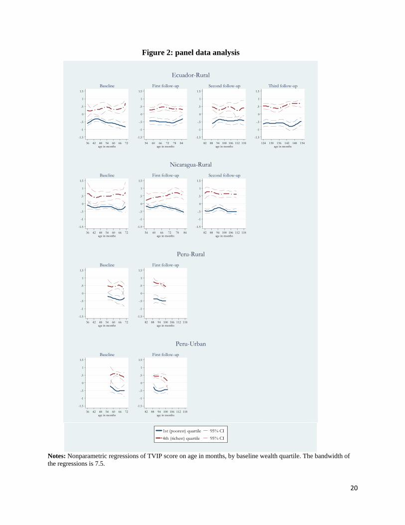
We next present the results from nonparametric (Fan) regressions (Fan and Gijbels 1996)
of the difference in scores between children in the top and bottom quartiles, and the associated
confidence intervals constructed by bootstrapping. Figure 1 suggests that the bulk of the
difference between poorer and less poor children is apparent by age 3 years in all countries;
Appendix Figure 2 shows that this is also the case in comparisons between the poorest and
richest deciles. We note, however, that making comparisons of age gaps in test scores measured
in standard deviations is not straightforward when the tests are measured with error. Suppose, as
seems likely, that there is more measurement error in the TVIP at younger ages (for example, if
younger children are more easily distracted). In this case, a finding of a constant gap in standard
deviations of test scores as children age would be consistent with a decline in the actual (as
opposed to measured) gap as children age.4
We conduct a number of robustness checks on our main results (Table 3). First, for four
countries (Colombia, Ecuador, Nicaragua, and Peru) we present results in which we use a
common set of household assets, rather than the largest set of assets available in the surveys for
each country, to construct our measure of wealth. (We cannot do this for Chile because there are
very few assets that are common to the Chilean and other data sets.) Second, for two countries in
which consumption data are available (Colombia and Nicaragua), we sort households into
quartiles using household per capita consumption, rather than wealth. Third, we compare
outcomes for children of mothers with incomplete primary education or less and those with 4 We thank an anonymous referee for pointing this out to us.

6
complete secondary education or more. Fourth, we restrict the sample to children of monolingual
parents.5 Fifth, we report results that use the norms provided by the test-developers (rather than
the internal z-scores we construct) to standardize the TVIP.6
Table 3 shows that the patterns summarized above are robust. Results are very similar
when only assets that are common across countries are used to construct the wealth index, or
when we use consumption, rather than wealth, as a measure of wellbeing. There are substantial
differences in child TVIP scores by mother schooling levels (incomplete primary or less,
compared to complete secondary or more) in all countries. For example, in rural Ecuador the
difference in outcomes between children of mothers with complete secondary schooling or more
and those with incomplete primary schooling or less is 1.16 standard deviations. Excluding
children in households where a language other than Spanish is spoken substantially increases the
wealth gradient in rural Peru (from 0.77 to 0.95 standard deviations), but has little effect on the
results for urban Peru, or urban or rural Ecuador.
Results that use the norms provided by the test developers (fifth row of the table) show
similar wealth gradients as those we report in our main specification. Recall that the distribution
of wealth in the data we use to calculate the TVIP scores is broadly similar to the distribution of
wealth in nationally representative surveys for the rural areas of all five countries, and for the
urban areas of Chile and Colombia. We can therefore also use these results to make (cautious)
comparisons across rural-urban areas in these two countries and across rural areas in all five
countries.
First, limiting the sample to rural areas, mean scores are highest in Chile (90 points),
substantially lower in Colombia and Ecuador (78 and 75 points, respectively), and lower still in
Peru and Nicaragua (69 and 66 points, respectively). This means that, in Nicaragua and Peru, the
average child in the poorest wealth quartile in rural areas has TVIP scores that are more than two
standard deviations below the reference population that was used to norm the test. The results for
5 In Peru, the TVIP was translated into Quechua, an indigenous language spoken primarily in rural areas of the highlands, and children were given the option of taking the test in Spanish or Quechua. Twenty-two percent of children in rural areas, but only 0.1 percent of children in urban areas, chose to take the test in Quechua. Because children in households that speak Quechua or another indigenous language may have more limited vocabularies in any given language, and because the likelihood of being a non-Spanish speaker is correlated with household wealth, we exclude children with mothers who report they speak a language other than Spanish in Peru (56 percent and 17 percent in rural and urban areas, respectively) and Ecuador (2 percent in both urban and rural areas). 6 The TVIP has been standardized by the test developers on samples of Mexican and Puerto Rican children to have an average score of 100 and a standard deviation of 15 at all ages. The lowest standardized score is 55.

7
Peru are particularly noteworthy because GDP per capita levels in Peru are roughly comparable
to those found in Colombia and Ecuador, and are approximately three times as high as those in
Nicaragua. Second, children in urban areas have somewhat higher scores than those in rural areas
in Chile (a difference of 6 points for those in the highest quartile), and substantially higher scores
in Colombia (a difference of 26 points, more than 1.5 standard deviations, for those in the
highest quartile). Of course, in interpreting these urban-rural comparisons, it is important to keep
in mind that average income levels tend to be substantially higher in urban than in rural areas in
most Latin American countries.
We also test the degree to which our results are sensitive to missing test data by
calculating upper and lower bounds on the wealth gradients (last row of Table 3), in the spirit of
Manski (1990) and Horowitz and Manski (2000). Specifically, we estimate the upper bound by
excluding all children with missing test data in the richest wealth quartile, and assigning a score
of zero to all children in the poorest wealth quartile who were missing the TVIP, as before.
Conversely, we estimate the lower bound by excluding all children with missing test data in the
poorest wealth quartile, and assigning a score of zero to all children in richest wealth quartile
who were missing the TVIP, as before. Table 3 shows that the bounds that take account of
missing test data are generally quite tight. For example, in urban Chile, our basic estimate
suggests that the difference in outcomes between children in the first and fourth wealth quartiles
is 0.78 standard deviations, the lower bound on this difference is 0.74, and the upper bound is
0.83. Only in Nicaragua, the country with the largest number of children with missing test data,
are the bounds somewhat wider, with a lower bound for the difference of 0.59 standard
deviations and an upper bound of 0.99 standard deviations.
Although the aim of our paper is descriptive, and the data we have do not allow us to
establish causality from socioeconomic status (whether measured by wealth, consumption or
education) to child cognitive development, we make an attempt to deepen our understanding of
the gradients we observe by carrying out some basic Oaxaca-Blinder decompositions.
Specifically, we divide each of the samples for a given country and area (urban or rural) into
children below and above the median level of wealth (Groups 1 and 2, respectively). We then
closely follow Blinder (1973), and calculate the proportion of the total difference in outcomes
between the two groups that can be attributed to differences in endowments (in our case, wealth),
the difference in the returns to these endowments, and the unexplained portion of the differential

8
(the difference in the intercepts). We carry out this decomposition with and without location
fixed effects (states in Chile, communities or census tracts in the other four countries). The
results from these decompositions are presented in Table 4.
We begin with a discussion of the results without location fixed effects (which are
comparable to other results in the paper). The top panel of the table shows that, in 6 out of 9
cases (rural Chile, Ecuador and Nicaragua; urban Chile, Ecuador, and Peru), between 75 percent
and 86 percent of the difference in TVIP scores between richer and poorer households is
accounted for by differences in wealth endowments; in another case, urban Colombia,
differences in endowments can account for the full difference in TVIP scores. Differences in the
returns to wealth between Groups 1 and 2 are generally small.
On the other hand, the returns to wealth appear to be substantially higher among poorer
households in the rural areas of Colombia and Peru. The overall difference in TVIP scores masks
this difference in the returns. We do not know why the returns to wealth in the rural areas of
Colombia and Peru would be different from those found in the rural areas of Chile, Ecuador, and
Nicaragua. It is possible that more in-depth qualitative work would be informative. In the
absence of such work, we cautiously conclude that, in most of the settings we study, the bulk of
the difference in TVIP scores between richer and poorer households can be accounted for by the
difference in endowments rather than differences in returns.
We next turn to the results that include location fixed effects, reported in the lower panel
of Table 4. Including these fixed effects substantially reduces the difference in TVIP scores
between richer and poorer households in Colombia, Ecuador and Nicaragua. This suggests that,
in these three countries, a substantial portion of the socioeconomic gradients in cognitive
development can be accounted for by residential sorting. Once we limit the comparisons to
children who live in the same location, the gap between richer and poorer households is
substantially smaller.
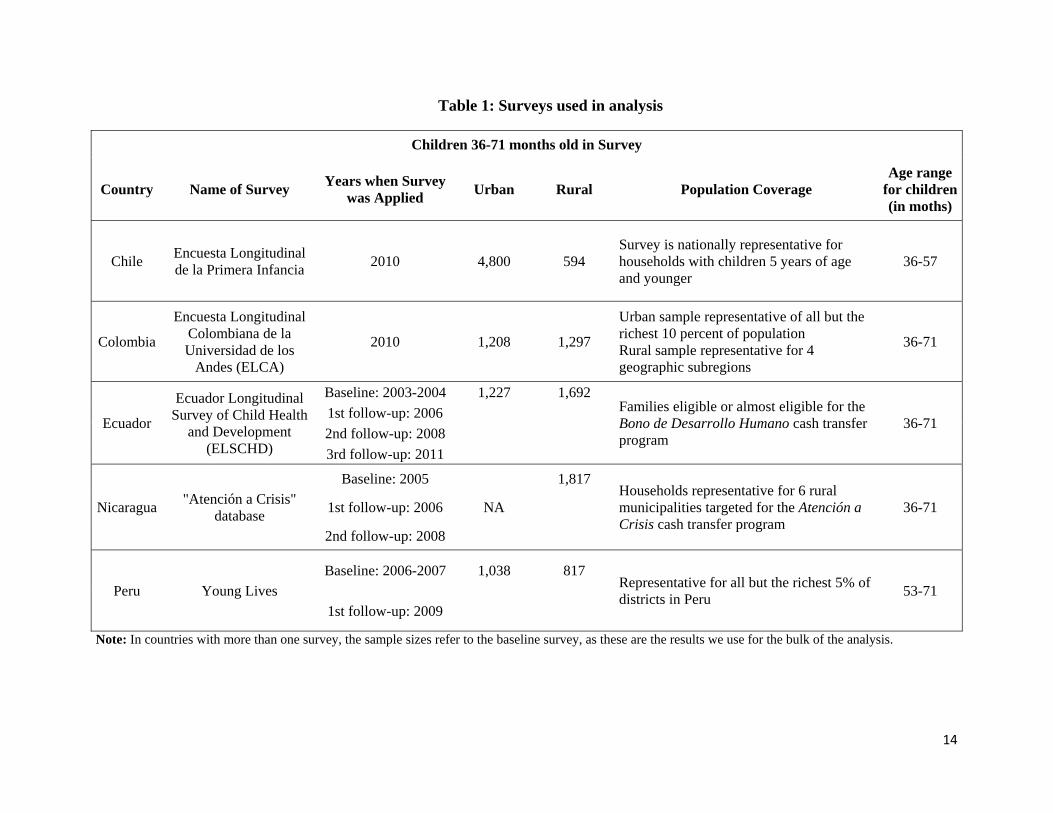
Finally, we use longitudinal data from rural Ecuador, rural Nicaragua, and rural and
urban Peru to analyze possible changes in the wealth gradients as children age. For this analysis,
we limit the sample to children who took the TVIP in all four survey waves in Ecuador (85
percent of children who took the TVIP at baseline), three survey waves in Nicaragua (92
percent), and two survey waves in Peru (96 percent). Figure 2 shows that in all three countries
the wealth gradients that are apparent among 4-5 year old children are also apparent as these

9
children age. In Ecuador, where the panel has the longest duration (7 years), differences in TVIP
scores between wealthier and less wealthy children at 12-13 years of age, when children are of
an age where they would be completing elementary school, are very similar to those found at 5-6
years of age. In all three countries, there is no evidence of catch-up. On the other hand, the
poorest children do not appear to fall further behind either.7
4. Discussion and conclusions Early childhood development has long-lasting consequences for adult success. Long-term panels
that have followed children from early ages into adulthood show that children with poor levels of
nutrition, inadequate cognitive development, and low levels of socio-emotional development
tend to do badly in school, have higher levels of unemployment, earn lower wages (even
controlling for schooling attainment), have a higher incidence of teenage pregnancy, are more
likely to use drugs, are more likely to be involved in criminal activities, and have children with
worse nutritional status.
Evidence on the extent to which there are shortfalls and socioeconomic gradients in
cognitive development among young children in developing countries is very scarce. In this
paper we use data from five countries in Latin America to show that there are important
differences in early language development between children in wealthier and poorer households.
Latin America is generally regarded as the most unequal region in the world (World Bank 2005).
Our analysis suggests that the differences in income levels and in other measures of wellbeing
that are apparent in adulthood arise early in children’s lives.
Our study has limitations. The lack of nationally-representative data for some countries
and the lack of urban data for Nicaragua limit our comparisons. Also, our wealth measure is
based on correlations of patterns of asset ownership and dwelling characteristics but does not
include a complete list of assets and dwelling characteristics, and does not consider that such
characteristics have different values (prices). Finally, we are able to compare only one measure
of cognitive development across countries.
Nevertheless, the strengths of our study are considerable. It is the first systematic, multi-
country comparison of wealth gradients in cognitive development for young children in the
7 Of course, in the presence of noisy data, one must be cautious about interpreting these panel results for the same reason one must be cautious about interpreting age-patterns based on a single cross-section.

10
developing world over critical periods of their life courses. The gradients we observe are
substantial. There are also large differences across countries in levels of child cognitive
development. In the three countries where we can follow children over time, there do not appear
to be substantive changes in the gradients once children enter school. This pattern, whereby
socioeconomic gradients appear early and are largely unchanged after age 6 years, is similar to
findings from the United States (Carneiro and Heckman 2003; Cunha and Heckman 2007;
Brooks-Gunn at al. 2006).
Our results have important policy implications. They reinforce with much more direct
evidence the importance of programs directed towards poor young children in developing
countries emphasized in a prominent recent survey (Engle et al. 2011). Nevertheless, they also
lead us to be somewhat pessimistic about closing these gaps because the magnitudes of the
differential we find are large relative to the program effects that have been estimated in the
literature. Berlinski et al. (2009) estimate that preschool attendance improves cognitive
development by 0.23 standard deviations in Argentina; cash transfers to very poor households
improve cognitive development by 0.18 standard deviations in Ecuador (Paxson and Schady
2010), and 0.10 standard deviations in Nicaragua (Macours et al. 2012); home visits are
estimated to improve cognitive development of young children by approximately 0.25 standard
deviations in Colombia (Attanasio et al. 2012). In this paper, we estimate that the difference
between children in the poorest and the richest quartile in the countries we study are bigger than
one standard deviation in urban Colombia and rural Ecuador, and larger than 0.75 standard
deviations in the urban and rural areas of all five countries (with the exception of rural Colombia,
where the difference is 0.57 standard deviations). Differences between children in the top and
bottom deciles are of course even larger. The results in our paper underline the magnitude of the
challenge faced by policy-makers seeking to close the gaps in development in early childhood in
Latin America and, we suspect, in many other developing countries.

11
References
Almond, Douglas, and Janet Currie. 2011. "Human Capital Development before Age Five." In Orley Ashenfelter and David Card, eds., Handbook of Labor Economics. North Holland: Amsterdam, pp. 1315-486.
Attanasio, Orazio, Emla Fitzsimons, Camila Fernández, Sally Grantham-McGregor, Costas Meghir, and Marta Rubio-Codina. 2012. “Stimulation and Early Childhood Development in Colombia: The Impact of a Scalable Intervention.” Paper presented at “Promises for Preschoolers: Early Childhood Development and Human Capital Accumulation” Conference, University College London.
Behrman, Jere, Lia Fernald, and Patrice Engle. 2013. "Preschool Programs in Developing Countries." P. Glewwe, Education Policy in Developing Countries. Chicago: University of Chicago Press.
Berlinski, Samuel, Sebastian Galiani, and Paul Gertler. 2009. “The Effect of Pre-Primary Education on Primary School Performance.” Journal of Public Economics 93(1-2): 219-234.
Blinder, Alan S. 1973. “Wage discrimination: Reduced form and structural estimates.” Journal of Human Resources 8(4): 436–455.
Brooks-Gunn, Jeann, Flavio Cunha, Greg Duncan, James Heckman, and Aaron Sojourner. 2006. “A Reanalysis of the IHDP Program.” Unpublished manuscript, Infant Health and Development Program, Northwestern University, 2006.
Carneiro, Pedro, and James Heckman. 2003. “Human Capital Policy.” NBER Working Paper 9495.
Case, Anne, and Christina Paxson. 2008. “Stature and Status: Height, Ability, and Labor Market Outcomes.” Journal of Political Economy 116(3): 499-532.
Cunha, Flavio, James Heckman and Lance Lochner. 2006. “Interpreting the Evidence on Life Cycle Skill Formation.” In Eric Hanushek and Finis Welch, eds., Handbook of the Economics of Education. North Holland: Amsterdam, pp. 697–812.
Cunha, Flavio, and James Heckman. 2007. “The Technology of Skill Formation.” American Economic Review 97(2): 31-47.
Duncan, Greg J., and Katherine Magnuson. 2013. “Investing in Preschool Programs.” Journal of Economic Perspectives 27(2): 109-32.
Dunn, Lloyd M., Delia E. Lugo, Eligio R. Padilla, and Leota M. Dunn. 1986. Test de Vocabulario en Imágenes Peabody. Circle Pines, MN: American Guidance Service.

12
Engle, Patrice, Maureen Black, Jere Behrman, Meena Cabral de Mello, Paul Gertler, Lydia Kapiriri, Reynaldo Martorell, and Mary Eming Young. 2007. “Strategies to Avoid the Loss of Developmental Potential in More Than 200 Million Children in the Developing World.” The Lancet 369(9557): 229-42.
Engle, Patrice, Lia Fernald, Harold Alderman, Jere Behrman, Chloe O'Gara, Aisha Yousafzai, Meena Cabral de Mello, Melissa Hidrobo, Nurper Ulkuer, Ilgi Ertem, S, Iltus, and the Global Child Development Steering Group. 2011. “Strategies for Reducing Inequalities and Improving Developmental Outcomes for Young Children in Low and Middle Income Countries.” The Lancet 378(9799): 1339-53.
Fan, Jianqing, and Irene Gijbels. 1996. Local polynomial modeling and its applications. Chapman and Hall, London.
Fernald, Lia, Ann Weber, Emmanuela Galasso, and Lisy Ratsifandrihamanana. 2011. “Socioeconomic Gradients and Child Development in a Very Low Income Population: Evidence from Madagascar.” Developmental Science 14(4): 832-47.
Heckman, James. 2008. “Schools, Skills, and Synapses.” Institute for the Study of Labor (IZA) Discussion Paper 3515.
Horowitz, Joel, and Charles Manski. 2000. “Nonparametric Analysis of Randomized Experiments with Missing Covariate and Outcome Data.” Journal of the American Statistical Association 95(449): 77-84.
Macours, Karen, Norbert Schady, and Renos Vakis. 2012. “Cash Transfers, Behavioral Changes, and Cognitive Development in Early Childhood: Evidence from a Randomized Experiment.” American Economic Journal: Applied Economics 4(2): 247-73.
Manski, Charles. 1990. “Nonparametric Bounds on Treatment Effects. American Economic Review 80(2): 319-23.
Naudeau, Sophie, Sebastian Martínez, Patrick Premand, and Deon Filmer. 2011. “Cognitive Development among Young Children in Low-Income Countries. In No Small Matter: The Impact of Poverty, Shocks, and Human Capital Investments in Early Childhood Development, Harold Alderman, ed., The World Bank, Washington, DC.
Paxson, Christina, and Norbert Schady. 2007. “Cognitive Development among Young Children in Ecuador: The Roles of Wealth, Health, and Parenting.” Journal of Human Resources 42(1): 49-84.
Paxson, Christina, and Norbert Schady. 2010. “Does Money Matter? The Effects of Cash Transfers on Child Development in Rural Ecuador.” Economic Development and Cultural Change 59(1):187-229.

13
Powell, Douglas R., and Karen E. Diamond. 2012. “Promoting Early Literacy and Language Development.” In Handbook of Early Childhood Education, Robert C. Pianta, ed., The Guilford Press, New York and London.
Schady, Norbert. 2011. “Parental Education, Vocabulary, and Cognitive Development in Early Childhood: Longitudinal Evidence from Ecuador.” American Journal of Public Health 101(12): 2299-307.
World Bank. 2005. Equity and Development, World Development Report 2006, Washington, D.C.
14
Table 1: Surveys used in analysis
Children 36-71 months old in Survey
Country Name of Survey Years when Survey was Applied Urban Rural Population Coverage
Age range for children (in moths)
Chile Encuesta Longitudinal de la Primera Infancia 2010 4,800 594
Survey is nationally representative for households with children 5 years of age and younger
36-57
Colombia
Encuesta Longitudinal Colombiana de la Universidad de los
Andes (ELCA)
2010 1,208 1,297
Urban sample representative of all but the richest 10 percent of population Rural sample representative for 4 geographic subregions
36-71
Ecuador
Ecuador Longitudinal Survey of Child Health
and Development (ELSCHD)
Baseline: 2003-2004 1,227 1,692 Families eligible or almost eligible for the Bono de Desarrollo Humano cash transfer program
36-71 1st follow-up: 2006 2nd follow-up: 2008 3rd follow-up: 2011
Nicaragua "Atención a Crisis" database
Baseline: 2005
NA
1,817 Households representative for 6 rural municipalities targeted for the Atención a Crisis cash transfer program
36-71 1st follow-up: 2006
2nd follow-up: 2008
Peru Young Lives Baseline: 2006-2007 1,038 817
Representative for all but the richest 5% of districts in Peru 53-71
1st follow-up: 2009
Note: In countries with more than one survey, the sample sizes refer to the baseline survey, as these are the results we use for the bulk of the analysis.

15
Table 2: Main results
Chile Colombia Ecuador Nicaragua Peru
Urban Rural Urban Rural Urban Rural Rural Urban Rural
Wealth quartile
Richest quartile 0.42 0.47 0.77 0.25 0.46 0.63 0.52 0.50 0.43 Poorest quartile -0.36 -0.42 -0.46 -0.32 -0.41 -0.58 -0.25 -0.45 -0.35 Difference 0.78 0.89 1.23 0.57 0.87 1.21 0.77 0.95 0.77 t-statistic 12.28 7.64 13.96 7.58 9.41 8.27 6.51 8.12 5.29
Note: Clustering of standard errors is done at community or census tract level (Colombia, Ecuador, Nicaragua, Peru) and state level (Chile). The calculation of the mean scores gives equal weight to each month of age, within a country and by place of residence (urban or rural).

16
Table 3: Robustness checks and extensions
Chile Colombia Ecuador Nicaragua Peru Urban Rural Urban Rural Urban Rural Rural Urban Rural
Common set of assets*
Richest quartile 0.79 0.44 0.51 0.62 0.40 0.47 0.43
Poorest quartile -0.48 -0.25 -0.39 -0.54 -0.20 -0.56 -0.34
Difference 1.27 0.69 0.90 1.16 0.60 1.03 0.77
t-statistic 10.68 6.57 9.22 8.09 5.29 10.74 5.30
Consumption
Richest quartile 0.88 0.49 0.42
Poorest quartile -0.43 -0.23 -0.21 Difference 1.31 0.72 0.63
t-statistic 13.03 6.55 5.37
Education
Highest education 0.16 0.27 0.32 0.44 0.46 0.60 1.12 0.33 0.63
Lowest education -0.52 -0.33 -0.65 -0.23 -0.42 -0.56 -0.10 -0.80 -0.15 Difference 0.68 0.60 0.97 0.68 0.88 1.16 1.21 1.13 0.78
t-statistic 8.97 4.14 10.48 5.04 7.40 9.20 5.58 9.52 6.08 Children with monolingual
Spanish-speaking mothers
Richest quartile 0.46 0.63 0.52 0.48
Poorest quartile -0.39 -0.57 -0.40 -0.47
Difference 0.85 1.20 0.91 0.95
t-statistic 9.05 8.30 7.52 4.44
Using external norms
Richest quartile 112.36 106.70 113.3 86.92 89.29 99.02 73.03 106.82 83.55 Poorest quartile 96.65 90.32 88.55 78.29 73.62 75.08 65.62 86.99 69.20 Difference 15.72 16.38 24.75 8.63 15.67 23.94 7.41 19.83 14.35 t-statistic -6.63 -6.70 -13.15 -6.86 -9.24 -8.23 -5.98 -8.47 -5.10
Lower and upper bound
Richest quartile (0.38 , 0.43) (0.41 , 0.52) (0.76 , 0.79) (0.24 , 0.25) (0.39 , 0.61) (0.57 , 0.68) (0.35 , 0.63) (0.49 , 0.51) (0.35 , 0.51) Poorest quartile (-0.36 , -0.40) (-0.39 , -0.46) (-0.46 , -0.47) (-0.31 , -0.32) (-0.33 , -0.46) (-0.50 , -0.60) (-0.23 , -0.36) (-0.37 , -0.47) (-0.29 , -0.43) Difference (0.74 , 0.83) (0.80 , 0.98) (1.22 , 1.27) (0.55 , 0.57) (0.72 , 1.07) (1.07 , 1.28) (0.59 , 0.99) (0.85 , 0.98) (0.64 , 0.93) t-statistic (11.40 , 15.70) (7.90 , 7.80) (13.70 , 14.60) (7.30 , 7.60) (7.30 , 11.10) (7.20 , 8.80) (5.00 , 8.00) (8.00 , 8.50) (3.80 , 6.60)

17
*Assets include: car, type of floor, type of walls, electricity, access to piped water, possession of cooking gas and refrigerator. Note: Clustering of standard errors is done at the community or census tract level (Colombia, Ecuador, Nicaragua, Peru) and state level (Chile). The calculations of the mean scores give equal weight to each month of age, within a country and by place of residence (urban or rural). The fraction of mothers with incomplete primary or less education is 3.5% for urban Chile, 7.8% for rural Chile, 12.3% for urban Colombia, 38.5% for rural Colombia, 14.3% for urban Ecuador, 20.1% for rural Ecuador, 68.5% for rural Nicaragua, 11.1% for urban Peru and 51.3 for rural Peru. The fraction of mothers with complete secondary education or more is 66.3% for urban Chile, 42.5% for rural Chile, 53.5% for urban Colombia, 14.9% for rural Colombia, 26.5% for urban Ecuador, 23.8% for rural Ecuador, 3.7% for rural Nicaragua, 56.5% for urban Peru and 13% for rural Peru. Children of mothers who speak only Spanish account for 83% of the sample in urban Peru, 44.2% in rural Peru, 98.7% in urban Ecuador 98.8% in rural Ecuador.

18
Table 4: Oaxaca-Blinder Decomposition of Differences
Chile Colombia Ecuador Nicaragua Peru Urban Rural Urban Rural Urban Rural Rural Urban Rural
No Fixed Effects
Endowments -0.39 -0.60 -0.74 -1.04 -0.44 -0.71 -0.32 -0.55 -0.92 Coefficients -0.07 0.02 -0.05 0.54 -0.20 -0.06 -0.04 -0.04 0.36 Unexplained -0.06 -0.08 0.06 0.02 0.08 -0.05 -0.07 -0.07 -0.02 Total difference -0.52 -0.66 -0.74 -0.48 -0.56 -0.82 -0.42 -0.65 -0.58
Fixed Effects
Endowments -0.38 -0.42 -0.37 -0.52 -0.28 -0.29 -0.03 -0.42 -0.37 Coefficients -0.09 -0.06 -0.29 0.27 -0.12 -0.02 -0.13 -0.08 0.13 Unexplained -0.05 -0.06 0.40 -0.11 0.06 -0.02 -0.05 -0.05 -0.37 Total difference -0.52 -0.55 -0.26 -0.37 -0.34 -0.32 -0.22 -0.55 -0.61
Note: Group 1 = below wealth median, Group 2: above wealth median. Clustering of standard errors is done at community or census tract level (Colombia, Ecuador, Nicaragua, Peru) and state level (Chile). Fixed Effects estimates include community or census tract (Colombia, Ecuador, Nicaragua, Peru) and region (Chile) dummy variables. The calculation of the mean scores gives equal weight to each month of age, within a country and by place of residence (urban or rural).

19
Figure 1: Age patterns in scores
Notes: Nonparametric regressions of TVIP score on age in months, by wealth quartile. The bandwidth of the regressions is 7.5.
-1.5
-1.2
-.9
-.6
-.3
0
.3
.6
.9
1.2
1.5
36 42 48 54 60 66 72age in months
Chile
-1.5
-1.2
-.9
-.6
-.3
0
.3
.6
.9
1.2
1.5
36 42 48 54 60 66 72age in months
Colombia
-1.5
-1.2
-.9
-.6
-.3
0
.3
.6
.9
1.2
1.5
36 42 48 54 60 66 72age in months
Ecuador
-1.5
-1.2
-.9
-.6
-.3
0
.3
.6
.9
1.2
1.5
36 42 48 54 60 66 72age in months
Nicaragua
-1.5
-1.2
-.9
-.6
-.3
0
.3
.6
.9
1.2
1.5
36 42 48 54 60 66 72age in months
Peru
Rural areas
-1.5
-1.2
-.9
-.6
-.3
0
.3
.6
.9
1.2
1.5
36 42 48 54 60 66 72age in months
Chile
-1.5
-1.2
-.9
-.6
-.3
0
.3
.6
.9
1.2
1.5
36 42 48 54 60 66 72age in months
Colombia
-1.5
-1.2
-.9
-.6
-.3
0
.3
.6
.9
1.2
1.5
36 42 48 54 60 66 72age in months
Ecuador
-1.5
-1.2
-.9
-.6
-.3
0
.3
.6
.9
1.2
1.5
36 42 48 54 60 66 72age in months
Peru
Urban areas
1st (poorest) quartile 95% CI
4th (richest) quartile 95% CI
20
Figure 2: panel data analysis
Notes: Nonparametric regressions of TVIP score on age in months, by baseline wealth quartile. The bandwidth of the regressions is 7.5.
-1.5
-1
-.5
0
.5
1
1.5
36 42 48 54 60 66 72age in months
Baseline
-1.5
-1
-.5
0
.5
1
1.5
54 60 66 72 78 84age in months
First follow-up
-1.5
-1
-.5
0
.5
1
1.5
82 88 94 100 106 112 118age in months
Second follow-up
-1.5
-1
-.5
0
.5
1
1.5
124 130 136 142 148 154age in months
Third follow-up
Ecuador-Rural
-1.5
-1
-.5
0
.5
1
1.5
36 42 48 54 60 66 72age in months
Baseline
-1.5
-1
-.5
0
.5
1
1.5
54 60 66 72 78 84age in months
First follow-up
-1.5
-1
-.5
0
.5
1
1.5
82 88 94 100 106 112 118age in months
Second follow-up
Nicaragua-Rural
-1.5
-1
-.5
0
.5
1
1.5
36 42 48 54 60 66 72age in months
Baseline
-1.5
-1
-.5
0
.5
1
1.5
82 88 94 100 106 112 118age in months
First follow-up
Peru-Rural
-1.5
-1
-.5
0
.5
1
1.5
36 42 48 54 60 66 72age in months
Baseline
-1.5
-1
-.5
0
.5
1
1.5
82 88 94 100 106 112 118age in months
First follow-up
Peru-Urban
1st (poorest) quartile 95% CI
4th (richest) quartile 95% CI

21
Appendix Table 1: Housing Conditions and Assets used for construction of wealth index
Chile Colombia Ecuador Nicaragua Peru Piped Water x x x x Gas x x x x Type of Toilet x x x x Electricity x x x Landline Phone x x Mobile Phone x x Access to Internet x x Type of Shower x Access to Hot Water x Sewer System x Garbage Elimination System x Exclusive Place for Cooking x Private Place for Cooking x Type of Cooking Fuel x Rooms in Dwelling x Owns House x Owns Working Animals x Floor Material x x x x x Walls Material x x x x Roof Material x x x Washing Machine x x x x Dryer Machine* x Refrigerator x x x x Fridge x x Microwave x x x Stove x x Mixer x x Blender x x Oven x Personal Computer x x x TV x x Color TV x Cable TV x x DVD x VHS or DVD x Video Camera x x Record Player x Video Games x Stereo x x Radio x x Car x x x Jeep x Motorbike x x Bicycle x Iron x x Fan x x Fumigator x Shredder x Floor Polisher x Loom** x Sewing Machine x Water Heater* x *Only used in urban sample **Only used in rural sample

22
Appendix Table 2: Main results
Chile Colombia Ecuador Nicaragua Peru
Urban Rural Urban Rural Urban Rural Rural Urban Rural
Wealth decile
Richest decile 0.52 0.44 0.91 0.26 0.73 0.98 0.76 0.85 0.78 Poorest decile -0.48 -0.60 -0.73 -0.47 -0.57 -0.65 -0.29 -0.72 -0.39 Difference 1.00 1.04 1.64 0.73 1.30 1.64 1.05 1.56 1.17 t-statistic -9.83 -6.47 -12.57 -5.72 -8.52 -11.38 -7.27 -13.38 -6.28
Note: Clustering of standard errors is done at community (Colombia, Ecuador, Nicaragua, Peru) and region level (Chile). The calculation of the mean scores gives equal weight to each month of age, within a country and by place of residence (urban or rural).

23
Appendix Figure 1: Distribution of wealth in survey used to calculate TVIP scores and nationally-representative surveys
Notes: Nationally representative surveys used: Chile, CASEN (2009); Colombia, GEIH (2009); Ecuador, ENEMDU, (2007); Nicaragua, EMNV (2005); Peru, ENAHO (2009). List of common assets used in each country. Chile: refrigerator, washing machine, mobile telephone, access to internet, cable TV, type of floor and personal computer. Colombia: access to piped water, car, electricity, refrigerator, type of walls, type of floor, landline telephone, TV, personal computer, exclusive place for cooking, stereo, oven, microwave, access to internet, motorbike and cable TV. Ecuador: access to piped water, car, electricity, refrigerator, type of floor, blender, TV, personal computer, stereo, VHS or DVD, washing machine, rooms in dwelling and type of shower. Nicaragua: access to piped water, car, electricity, refrigerator, type of walls, type of floor, type of roof, type of toilet, radio and fan. Peru: access to piped water, type of walls, type of floor, type of roof, blender, TV, personal computer, iron, bicycle, motorbike, radio, washing machine, landline telephone and mobile telephone.
Rural areas
Urban areas
4th (poorest) quartile 1st (richest) quartile
0.1
.2.3
-4 -2 0 2 4
Chile
0.1
.2.3
.4
-4 -2 0 2 4
Ecuador
0.1
.2.3
.4
-4 -2 0 2 4
Colombia
0.1
.2.3
.4
-4 -2 0 2 4
Peru
Household survey sample TVIP sample
0.1
.2.3
.4
-4 -2 0 2 4
Chile
0.1
.2.3
.4
-4 -2 0 2 4
Colombia
0.1
.2.3
.4
-4 -2 0 2 4
Ecuador
0.1
.2.3
.4.5
-4 -2 0 2 4
Nicaragua
0.2
.4.6
.8
-4 -2 0 2 4
Peru

24
Appendix Figure 2: Age patterns in scores
Notes: Nonparametric regressions of TVIP score on age in months, by wealth quartile. The bandwidth of the regressions is 7.5.
-1.5
-1
-.5
0
.5
1
1.5
2
36 42 48 54 60 66 72age in months
Chile
-1.5
-1
-.5
0
.5
1
1.5
2
36 42 48 54 60 66 72age in months
Colombia
-1.5
-1
-.5
0
.5
1
1.5
2
36 42 48 54 60 66 72age in months
Ecuador
-1.5
-1
-.5
0
.5
1
1.5
2
36 42 48 54 60 66 72age in months
Nicaragua
-1.5
-1
-.5
0
.5
1
1.5
2
36 42 48 54 60 66 72age in months
Peru
Rural areas
-1.5
-1
-.5
0
.5
1
1.5
2
36 42 48 54 60 66 72age in months
Chile
-1.5
-1
-.5
0
.5
1
1.5
2
36 42 48 54 60 66 72age in months
Colombia
-1.5
-1
-.5
0
.5
1
1.5
2
36 42 48 54 60 66 72age in months
Ecuador
-1.5
-1
-.5
0
.5
1
1.5
2
36 42 48 54 60 66 72age in months
Peru
Urban areas
1st (poorest) decile 95% CI10th (richest) decile 95% CI