NBER WORKING PAPER SERIES

WAVES IN SHIP PRICES AND INVESTMENT

Robin GreenwoodSamuel Hanson

Working Paper 19246http://www.nber.org/papers/w19246

NATIONAL BUREAU OF ECONOMIC RESEARCH1050 Massachusetts Avenue

Cambridge, MA 02138July 2013

We thank Andreas Beroutsos, Murray Carlson, Ben Esty, Fritz Foley, Fotis Giannakoulis, StefanoGiglio, Charlie Norz, David Scharfstein, Andrei Shleifer, Erik Stafford, Jeremy Stein, Martin Stopford,Larry Summers, Adi Sunderam and seminar participants at Columbia, Harvard, MIT, Princeton, theSFS Finance Cavalcade, and the Texas Finance Festival for helpful suggestions. We are grateful toJared Dourdeville for excellent research assistance and to Clarkson Research for providing data. Theviews expressed herein are those of the authors and do not necessarily reflect the views of the NationalBureau of Economic Research.

NBER working papers are circulated for discussion and comment purposes. They have not been peer-reviewed or been subject to the review by the NBER Board of Directors that accompanies officialNBER publications.

© 2013 by Robin Greenwood and Samuel Hanson. All rights reserved. Short sections of text, not toexceed two paragraphs, may be quoted without explicit permission provided that full credit, including© notice, is given to the source.

Waves in Ship Prices and InvestmentRobin Greenwood and Samuel HansonNBER Working Paper No. 19246July 2013JEL No. E44,G02,G12,L9

ABSTRACT

We study the returns to owning dry bulk cargo ships. Ship earnings exhibit a high degree of meanreversion, driven by industry participants’ competitive investment responses to shifts in demand. Shipprices are far too volatile given the mean reversion in earnings. We show that high current ship earningsare associated with high secondhand ship prices and heightened industry investment in fleet capacity,but forecast low future returns. We propose and estimate a behavioral model that can account for theevidence. In our model, firms over-extrapolate exogenous demand shocks and partially neglect theendogenous investment responses of their competitors. Formal estimation of the model confirms thatboth types of expectational errors are needed to account for our findings.

Robin GreenwoodHarvard Business SchoolBaker Library 267Soldiers FieldBoston, MA 02163and NBERrgreenwood@hbs.edu

Samuel HansonHarvard Business SchoolBaker Library 351Soldiers FieldBoston, MA 02163and NBERshanson@hbs.edu

An online appendix is available at:http://www.nber.org/data-appendix/w19246

1

I. Introduction

Dry bulk shipping is a highly volatile and cyclical industry in which earnings, investment,

and returns on capital appear in waves. In 2001, a 5-year old “Panamax” ship commanded daily

lease rates of $5,325 and could be purchased for $14 million. By December 2007, daily lease rates

had grown more than tenfold to $61,000, and purchase prices had risen more than fivefold to $89

million. By 2011, lease rates and secondhand prices had nearly returned to their 2001 levels. This

boom-bust cycle occurred alongside enormous fluctuations in industry investment. In December

2001, outstanding orders for new ships amounted to less than 10% of the active fleet. However, by

August 2008, outstanding orders for new ships exceeded 75% of the active fleet.

We study how cycles in investment, lease rates, and secondhand prices are connected to

predictable variation in the returns to ship owners. Using monthly data on secondhand ship prices

and ship lease rates between 1976 and 2011, we measure the payoffs to an investor who purchased a

dry bulk cargo ship in the secondhand market, operated it for a period of time, earning a cash flow

stream in the form of market-based lease rates, and later sold the ship. The annual realized returns to

owning a ship vary enormously over time, from a low of -76% between December 2007 and

December 2008 to a high of +86% between June 1978 and June 1979.

We show that returns to owning and operating a ship are predictable and closely related to

industry-wide investment in capacity. High current ship earnings are associated with higher ship

prices and higher industry investment, but predict low future returns on capital. Conversely, high

levels of ship demolitions—a measure of industry disinvestment—forecast high returns. The

economic magnitude of return predictability we uncover is large: our baseline regressions suggest

that expected one year forward excess returns range from -43% to +16%.

One should not be surprised that ship charter rates—the payment that a ship owner earns for

leasing out his ship—fluctuate significantly over time. The supply of bulk carriers is essentially

fixed in the short-run, because building and delivering a new ship takes between 18 and 36 months.

Coupled with inelastic demand for shipping services, this time-to-build problem means that

temporary imbalances between global demand for shipping services and the size of the fleet can

lead to large changes in ship charter rates.

At the same time, fluctuations in short-term charter rates do not imply anything about the

expected returns to owning and operating a ship. Consider the natural benchmark in which the

2

returns required by ship owners are constant over time. What is the competitive response to an

unexpected jump in shipping demand in such a setting? Charter rates would temporarily spike,

raising contemporaneous realized returns. But ship investors would respond to the spike in charter

rates by building additional ships. Over time, charter rates would fall back to their steady-state level

as additional ships were added to the fleet. The prices of used ships—which are long-lived capital

assets—would initially jump modestly in anticipation of heightened near-term cash flows, before

gradually returning to their steady-state level. In equilibrium, enough ships would be brought online

to bring the expected return to investing in new ships down to the required return. In short, the

combination of forward-looking rational behavior on the part of ship owners and competitive

industry dynamics would ensure that earnings exhibit a high degree of mean reversion but that

expected returns were constant. Rosen, Murphy, and Scheinkman (1994) explore dynamics of this

sort in their model of cattle cycles.

Although the rational expectations benchmark is appealing, the data suggest a more complex

story. Following a jump in demand, the ensuing glut of shipping supply pushes charter rates and

secondhand ship prices below the rational-expectations level, resulting in low realized returns to

ship owners during the subsequent bust. A simple calculation based on constant discount rates

suggests that at peaks, market participants may have overpaid for ships by more than 100 percent.

What can explain these results? A first possibility is that the return investors require for

owning and operating ships varies significantly over time, perhaps because ships are priced by

diversified investors whose attitudes toward risk fluctuate over the business cycle. In this case,

investment is high during booms, but prices are fair because investors require far lower returns

going forward. While one can never fully rule out this type of explanation, we argue that the

variation in expected returns is too large and too disconnected from well-understood cyclical drivers

of risk premia to be plausibly explained in this way.

We explore behavioral explanations in which there is too much investment in booms

because firms over-extrapolate abnormally high profits into the future. Models in which market

participants over-extrapolate exogenously given cash flows are well understood in economics (see

e.g., Barberis, Shleifer, and Vishny (1998), Rabin (2002), Barberis and Shleifer (2003)). But in

most industries, the cash flows are not exogenous but are an endogenous equilibrium outcome that

is impacted by the industry supply response to demand shocks. It follows that firms may over-

3

extrapolate current profits either because they (i) over-estimate the persistence of the exogenous

demand shocks facing the industry or (ii) fail to fully appreciate the long-run endogenous supply

response to those demand shocks.

In a competitive setting, both types of errors are plausible, and both errors feature in

narrative accounts of shipping history. Extrapolation of demand is related to the

“representativeness” heuristic, in which subjects draw strong conclusions from small samples of

data (Tversky and Kahneman (1974) and Rabin (2002)). Neglect of the long-run endogenous supply

response to demand shocks constitutes a form of over-optimism known as “competition neglect.”

Competition neglect has been documented in laboratory experiments (e.g., Camerer and Lovallo

(1999)). In these experiments, subjects in competitive settings overestimate their own skill and

speed in responding to common observable shocks and underestimate the skill and responsiveness

of their competitors. Specifically, following shocks which boost industry-wide profitability,

individuals enter the market too aggressively. Informal references to competition neglect appear in

many historical accounts of the dry bulk shipping industry (e.g., Metaxas (1971), Cufley (1972),

and Stopford (2009)). This is not surprising, because as Kahneman (2011) notes, competition

neglect can be particularly strong when firms receive delayed feedback about the consequences of

their decisions, as one would expected in industries with significant time-to-build delays.

We develop a simple q-theory model of investment dynamics in an industry in which firms

compete to produce homogenous services from a long-lived capital good—a ship in our case. We

start with the rational expectations benchmark in which firms correctly forecast the exogenous path

of future demand, and in which all firms properly anticipate the endogenous investment response of

other firms. In this benchmark case, neither ship prices nor investment are very volatile and returns

on capital are unpredictable by construction.

We introduce competition neglect into the model by assuming that each firm underestimates

the investment response of its rivals by a constant proportion. This implies that positive shocks to

demand generate excessive investment responses. This investment predictably depresses future

charter rates and ship prices, leading prices to overshoot their rational-expectations levels. Even

though the required return of shipping investors is constant in our model, investors’ tendency to

underestimate the competition generates predictable variation in returns.

4

We also allow firms to over-estimate the persistence of the exogenous demand process.

Similar to the case in which market participants display competition neglect, allowing for demand

extrapolation implies that high current levels of industry demand are associated with

overinvestment and low future returns. However, both biases are needed to fully understand the

dynamics of the shipping industry. For example, if industry participants extrapolate demand shocks,

but fully understand the competitive response of their peers, this will only generate limited excess

volatility in ship prices. This is because industry participants will only pay high prices if they

believe that high earnings will persist, which is largely equivalent to assuming that the competitive

response of peer firms will be muted. In this way, allowing for both biases helps us match the full

set of patterns we observe in ship earnings, prices, and returns.1

We estimate the model using the simulated method of moments (McFadden (1989)). In our

estimation, firms are allowed to suffer from both behavioral biases—over-extrapolation of the

exogenous demand process as well as neglect of the endogenous supply response. (We also show

restricted estimates, in which we constrain firms to be subject to only one of the two biases.) The

main parameters of interest are the degree of “competition awareness” among market participants

and the degree of demand over-extrapolation. We estimate the degree of competition awareness to

be about 50%. This means that ship owners do not fully anticipate the investment response of their

peers when reacting to demand shocks. At the same time, our estimates imply that market

participants are partially forward looking and anticipate a portion of the industry supply response.

We estimate the true persistence of demand shocks to be 0.68 on an annual basis, with market

participants behaving as if they believe persistence were closer to 0.80. By estimating the two

behavioral parameters of the model, we can infer how the beliefs of market participants change

following a shock to demand. We contrast the path of earnings, fleet size, and ship prices that

market participants expect with those that appear in our data. Our estimates suggest that modest

errors in expectations can result in dramatic excess volatility in earnings, prices, and investment.

Our paper is closely related to the cobweb model of industry cycles, first outlined by Kaldor

(1934, 1938) but explored empirically by many others (Freeman (1975), and Rosen, Murphy, and

1 Because our model considers a representative ship owner, we abstract away from the question of who is subject to the behavioral biases that we estimate in the data. This means that, for example, we do not consider heterogeneity in ship owner behavior or questions as to whether debt holders or equity holders are subject to the biases.

5

Scheinkman (1994))2. According to the cobweb theory, producers set quantities one period in

advance based on the naïve assumption that current prices will persist, generating oscillations in

price and quantity that converge to a steady state. The cobweb turns out to be a limiting case of our

model when firms completely neglect the competition. Our main contribution to this literature is to

show how price and investment dynamics are connected to the predictability of investment returns.

Even with moderate competition neglect, our model can generate excessive volatility in ship

earnings, secondhand prices, and investment along with the attendant return predictability.

Our findings are also related to an extensive literature in asset pricing that documents return

predictability in stock and bond markets (see Cochrane (2011) for a summary). In contrast with this

literature, we analyze the returns on real capital investment directly as opposed to the more common

approach of studying the returns on financial claims on corporate cash flows. Our work is also

related to recent papers on industrial structure and stock returns such as Hou and Robinson (2006)

and especially Hoberg and Phillips (2010), who study the role of industry competition in driving the

US stock market. Finally, we draw on Stopford (2009) and Kalouptsidi’s (2013) excellent analyses

of the dry bulk shipping industry.

The next section provides a brief overview of the dry bulk carrier industry and summarizes

our data. Section III summarizes the correlations between earnings, secondhand prices, investment,

and future returns. These correlations motivate a behavioral model of industry investment and price

cycles, which we develop in Section IV. Section V estimates the model using the simulated method

of moments. Section VI concludes.

II. Dry Bulk Carriers: Earnings, Prices, and Investment

Solid commodities are transported in large cargo ships known as bulk carriers. In 2011, bulk

carriers made up approximately 40% of the world’s shipping fleet (tankers and container ships

made up most of the rest) and had a combined cargo capacity of 609 million deadweight tonnes

(DWT) across 8,868 ships. These ships had a combined market value of roughly $180 billion in

2011, having peaked at $549 billion in June 2008.

2 See also Ezekiel (1938), Muth (1961), and Nerlove (1958).

6

The market for shipping cargo is highly competitive with hundreds of firms operating ships,

and no single firm owning more than a few percent of the fleet.3 In 2011, more than half of all bulk

carriers were owned by Greek, Japanese, or Chinese firms. The demand for shipping services is

volatile and is driven by the amount of seaborne trade which, in turn, is linked to the level of global

economic activity. However, the growth in seaborne trade is only weakly correlated with global

economic growth (Stopford (2009)). This is because the trade in bulk commodities—principally,

iron ore, coal, and grains—is impacted by evolving geographic trade patterns (the location of

commodity users in relation to commodity suppliers) and geopolitical events (e.g., the 1967-1975

Suez canal closure, the 1979 Iranian revolution, the 1990 Gulf War, and the 2003 Iraq War).

Demand for shipping services is generally thought to be fairly inelastic because there are few cost

effective alternatives for international transport of most bulk goods (Stopford (2009)).

We obtain monthly time-series data for 1976-2011 on the dry bulk shipping market from

Clarkson, the leading ship broker and provider of data to shipping market participants. Starting in

1976, Clarkson provides monthly estimates of charter rates and secondhand prices for various ship

sizes and vintages. In addition, we obtain monthly information on the composition of the fleet, as

well as data breaking out new additions to the fleet and demolition decisions. Beginning in 1996,

Clarkson provides the complete order book, which includes the number of ships on order,

deliveries, and cancellations. Since we require the future secondhand price in 12 months to compute

realized returns, our baseline sample runs from January 1976 to December 2010.

At the end of 2011, bulker fleet capacity was split between smaller ships (Handymax and

Handysize), mid-sized ships (Panamax), and larger ships (Capesize). As shown in Figure 1, the

share of bulk cargo carried by Panamax and Capesize ships has grown since the 1970s. However,

investment across different ship types has been highly synchronized over time. Panel B of Figure 1

shows that if we define investment as the 12-month percentage change in fleet capacity, there is a

high correlation between investment in the Panamax ship and fleet-wide investment. Based on this

observation and following Kalouptsidi (2013), we measure investment fleet-wide, abstracting away

from changes in the composition of the global cargo fleet. Since different ship sizes are close

3 There are few, if any, barriers to entry in dry-bulk shipping and few, if any, scale economies to operating a larger fleet. The average shipping firm in recent years only owns five ships (Stopford (2009)) and the top 19 owners (excluding the Chinese government-owned COSCO) held only 20% of industry capacity in 2006 (Bornozis (2006)).

7

substitutes in the services they provide, total fleet capacity is the relevant quantity to relate to ship

earnings and prices.4

A. Earnings, prices, and value

Ship owners earn income either by transporting cargo for hire or by leasing out their vessels

for a defined period of time in the “time charter” market. In this market, which is organized by a

large network of brokers such as Clarkson, a charterer pays the ship owner a daily “hire rate” for the

entire length of the contract, which is typically 12 months. The owner furnishes the charterer with

the ship and must pay the costs of the crew and maintenance capital expenditures, but the remaining

costs, including fuel, are borne by the charterer. In computing earnings and holding period returns,

we assume that the owner leases the ship out rather than operating it directly.5

Table I and Figure 2 show our time-series data on net earnings, defined as the real (constant

2011) dollars to be earned, net of costs, by leasing the ship over the next year. Clarkson provides us

with monthly estimates of the 12-month charter rate for many different ships, based on their polling

of brokers in the market as well as recent transactions.6 We focus on the 76,000 DWT Panamax

carrier. We use this ship because it is a fairly representative bulk carrier—neither the smallest nor

the largest vessel—and because we can construct consistent time series on both earnings and

secondhand prices for ships of this size over our full sample.

For a 5-year old ship, the owner earns the charter rate for an average of 357 days per year;

the boat is docked for maintenance for the remaining 8 days per year. Although the lessor pays fuel

and insurance, the ship owner must provide a crew at a daily real cost that we estimate to be

4 Earnings and prices are nearly perfectly correlated across different ship sizes in the time-series. For instance, the real price of 5-year old Capesize ships is 97% correlated with the price of Panamax carriers. Again, this supports the idea that, while bulk carriers vary in size, they provide a highly homogenous service. 5 While the time charter is by far the most frequent leasing arrangement (Stopford (2009)), other contractual arrangements are also possible. Specifically, owners can lease their ships in the “voyage” or “spot” charter market or in the market for a “contract of affreightment.” Prices for various contract types appear to be tightly integrated. Furthermore, there are a variety of distinct cargo shipping routes—e.g., Australia to China or Brazil to Europe. Demand for each route varies separately over time. Charter rates differ across routes in the very short-run. However, rates for different routes closely track each other because supply quickly flows toward routes with elevated rates. For example, the voyage charter rate for a Port Cartier to Rotterdam trip is 94% correlated with the average 1-year time charter rate for a Panamax carrier. Thus, using the average time charter rate as a proxy for cash flows is reasonable. 6 To verify data reliability, we obtained micro data on charter rates and prices for a sample of transactions between December 2009 and November 2012. Monthly averages of charter rates were 98.2% correlated with the hire rate series from Clarkson. The average sale price for 5-year old Panamax ships was 99.8% correlated with our price series.

8

approximately $6,000 per day in 2011 dollars. In addition, an owner incurs a maintenance and

depreciation expense. Thus real annual earnings are

357 365 ,t t t tDailyCharterRate DailyCrewCost Depreciation (1)

where DailyCharterRate, DailyCrewCost, and Depreciation are expressed in constant 2011 dollars

(i.e, all historical nominal values are converted to 2011 dollars using the US CPI index).

Depreciation is a constant adjustment we make to account for the fact that after 12 months, a 5-year

old ship is now a slightly less valuable 6-year old ship. We assume that the maintenance and

depreciation expense is 4% of the initial ship price, based on a 25-year ship life (1/25=4%). Because

depreciation is assumed to be a constant fraction of the initial price, this assumption only impacts

the average excess return on ships and otherwise has no impact on any of the results that follow. We

also compute gross earnings by dropping the depreciation term from equation (1). Our calculation

for earnings is an approximation, but it is confirmed by Stopford (2009), due diligence we

conducted with industry participants, and case studies of the shipping industry by Stafford, Chao,

and Luchs (2002) and Esty and Sheen (2012).

As can be seen in Figure 2, real ship earnings are highly volatile. Before 2002, annual real

earnings had a monthly standard deviation of $2.15 million, compared to a mean of $2.5 million.

Starting in 2002, volatility increased substantially to a monthly standard deviation of $5.4 million.7

In addition to illustrating the high volatility of ship earnings, Figure 2 shows the high degree

of mean reversion in earnings. Current earnings are 96% correlated with earnings in the following

month and only 20% correlated with earnings 12 months earlier. This high degree of estimated

mean reversion is not sensitive to the time period in question.

New ships can be ordered through shipyards or purchased on a used basis in a liquid

secondhand market. In recent years, at least 10% of the bulker fleet has traded on a secondary basis

each year (Kalouptsidi (2013)). According to Stopford (2009), adverse selection is not a significant

concern in this market.8 And, just as with many financial assets, there is a large common time-series

7 Recall that earnings are based on 12-month charter rates, so we are already examining a smoothed, forward-looking version of short-term spot charter rates, which are even more volatile. 8 Bulk carriers are like cars that always drive 60 miles-per-hour on an empty highway. Thus, age, mileage, and maintenance history—all of which are publicly observable—are sufficient statistics for value.

9

component of prices that is shared by ships of all sizes and ages.9 We focus on this common time-

series component and, as with earnings, proxy for this component using the price of a 5-year old

Panamax ship. We express the price in constant 2011 dollars. As shown in Figure 2, the real price

tracks real earnings extremely closely throughout the 1976-2010 period: the correlation is 87%.

Although real earnings and real prices are highly correlated, the ratio of earnings to price is

far from constant. When real earnings are high, real ship prices are also high but prices do not rise

quite as quickly, leading to a higher ratio of earnings to prices. This is what one would expect if

firms have some understanding that real earnings are mean reverting.10, 11

A simple way to evaluate the apparent volatility in ship pricing is to consider a benchmark

in which discount rates are constant. In the spirit of Shiller (1981), Figure 3 plots the actual time

series of market ship prices versus a simple model-implied present value of ship earnings based on a

constant 10% real discount rate.12 To calculate the present value, we assume that the buyer of a 5-

year old ship receives the current charter rate for 12 months following purchase, and then signs a

new charter for another 12 months thereafter. We estimate the rate on this new charter based on the

time-series autocorrelation of charter rates for the full sample. After this initial two year period, we

assume the buyer receives the average real gross earnings (again calculated over the full time

series). We make a proportional adjustment once the ship is 15 years old, reducing charter rates by

15%, because older ships tend to lease at lower prices (Stopford (2009)). Finally, we assume that

ships have a useful economic life of 25 years, so the 5-year old ship will be scrapped in 20 years

and the owner will receive a scrap value. The complete details of this calculation are provided in the

Internet Appendix.13

Figure 3 shows that the model-implied present value of the cash flows from a ship are

considerably less volatile than actual ship prices. Consistent with Shiller (1981) and subsequent

9 Kalouptsidi (2013) finds that the cross-sectional coefficient of variation of individual ship prices (cross-sectional standard deviation divided by the cross-sectional mean) is only 13% in the typical quarter over her 1998-2010 sample. 10 The growing perpetuity formula says /P = r – g where r is the required return and g is the expected earnings growth rate. Thus, if expected growth is low when the level of earnings is high, we would expect /P to be high at these times. 11 Both real ship earnings and the real price of ships appear to be stationary. Indeed, we can strongly reject the presence of a unit root in both series. At a 12-month horizon, the t-statistic for a test of the null that the auto-correlation of real earnings is 1 is t = –4.97. A similar test for real prices yields t = –2.69. This is natural: the real price for a mature good such as shipping services should be constant over the long-run in a multi-sector growth context. 12 A 10% discount rate ensures that the average model-based price is close to the actual time-series average of prices. 13 Internet Appendix available on both authors’ websites: http://www.people.hbs.edu/rgreenwood/shipsIA.pdf

10

work on the excess volatility of asset prices (e.g., Campbell (1991)), the standard deviation of

model-implied present values is $2.4 million, compared with a standard deviation of $14.9 million

for used ship market prices. This discrepancy is driven by the fact that the present value calculation

is not very responsive to changes in current earnings, which are expected to be almost completely

reverted away one year later. In contrast, actual market prices are extremely responsive to current

ship earnings. Taken together, this suggests that investors value ships as if they anticipate

considerably less mean reversion in earnings than there has been in the actual data.

B. Returns

Using earnings and prices, we can compute the holding period return for an investment in

ships. The 1-year holding period return on a ship is the 1-year change in the secondhand price, plus

the earnings accruing to an owner who signed a 12-month lease immediately after purchasing the

ship, scaled by the period t secondhand price

1 1( ) / ,t t t t tR P P P (2)

where P is the secondhand ships price and is defined according to equation (1). We use

secondhand prices instead of new prices because a buyer of a secondhand ship has immediate

access to the ship and thus rental income.14 As is common in asset-pricing studies, we forecast

excess returns as opposed to raw returns. Thus, our main dependent variable is the log excess return

on ships, defined as 1 1 , 1log(1 ) log(1 )t t f trx R R .15 Table 1 shows that holding period returns are

incredibly volatile: average 1-year excess returns are 6%, with a standard deviation of 32%.

To compute multi-year returns, we assume the ship owner signs a new 12-month time

charter at the prevailing rates each year. Thus, we can compute 2- and 3- year cumulative log excess

returns by simply summing 1-year log excess returns.

C. Investment plans: The order book

At the firm-level, investment occurs when a used ship is acquired from another owner or

when a new ship is purchased from a shipyard. At the industry-level, investment occurs only when a

14 A buyer of a new ship must wait 18-36 months for delivery, depending on workflow at shipyards. And time-to-build delays increase during shipbuilding booms (Kalouptsidi (2013)). Thus, a buyer could be justified in paying a higher price for a used than a new ship when current charter rates are high. Such a dynamic occurred in 2007-2008. 15 We measure the 12-month nominal return on riskless government bonds by cumulating the monthly RF series from Ken French. Since we subtract off the nominal riskless return, we compute nominal shipping returns in equation (2).

11

new ship is purchased. Industry supply is highly inelastic in the short-run due to time-to-build

delays.16 Beginning in 1996, Clarkson provides monthly data on the order book, which is the ledger

of ships that have been ordered at shipyards around the world. The order book evolves according to

1 .t t t t tOrders Orders Contracting Deliveries Cancel (4)

Thus, the change in the order book equals new orders in each month (Contracting), minus ships

delivered in that month (Deliveries), minus previous orders that were cancelled (Cancel). All items

in equation (4) are in DWT and reflect changes in the total industry-wide fleet capacity.

Based on equation (4), we construct two measures of investment plans, all scaled by current

fleet size: net contracting activity (i.e., contracting minus cancellations) over the past 12-months

(Contracting[t-1,t]/Fleett) and the size of the current order book (Orderst/Fleett). The average size of

the order book is 27% of the fleet during the 1996-2010 period for which we have order data.

D. Investment realizations: changes in fleet capacity

The fleet size evolves according to

1 ,t t t t t tFleet Fleet Deliveries Demolitions Conversions Losses (5)

with all terms expressed in DWT. Changes in the bulker fleet are primarily driven by deliveries

(when new ships come online and fall out of the order book) and demolitions (when old ships are

scrapped). Conversions and Losses capture rare incidents in which ships are repurposed from one

use to another (e.g., a tanker is converted to a bulk carrier), or ships are lost in accidents.

The Deliveries term in equation (5) represents the realization of past investment plans. Once

ordered, a ship typically takes 18 to 36 months to be built and delivered (Kalouptsidi (2013)).

Demolitions are driven by the aging of the fleet—as ships become older, they become more costly

to maintain and eventually they are no longer safe to use and must be scrapped. However, the

demolition of an old ship may be postponed when current lease rates are high and accelerated when

current lease rates are low. Thus, aggregate Demolitions partially reflect active disinvestment

decisions made by ship owners.

Panel A of Figure 4 shows deliveries and demolitions since 1976. The dashed line indicates

the net change in fleet-wide capacity, computed according to equation (5), and scaled by current

16Although the fleet size is fixed in the short run, industry voyage capacity is not totally fixed since ships can sail faster. Doing so is costly as it burns more fuel per mile traveled and results in additional wear and tear on a ship. So, while short-run supply is not perfectly inelastic, it is highly inelastic (Stopford (2009)).

12

fleet size. On average, the fleet has grown from a capacity of 100 million DWT at the start of our

sample to just over 600 million DWT in December 2011. The figure shows that when demolitions

are high, deliveries tend to be low a few years later. This reflects the time-to-build delay from

ordering to delivery. Panel B shows that deliveries commove strongly with lagged earnings: when

earnings are higher, more ships are ordered.

E. Shipping market cycles, 1976-present

Before proceeding with empirical analysis, we relate our time-series measures of earnings,

prices, and investment to narrative accounts of cycles in the bulk carrier industry. These accounts

are a useful reality check for our data, as well as providing insights into the psychology of market

participants during past shipping booms and busts.

Our sample begins in 1976 during the midst of what Stopford (2009) describes as a “very

depressed” leasing market. According to Stopford, demand for bulk shipping services grew rapidly

in 1979 and 1980 due to increased commodity trade and large-scale substitution from oil to coal

following the 1979 oil-price shock. And demand outstripped supply due to “low ordering during the

previous bust.” This boom lasted until early 1981 when a US coalminers’ strike and the onset of the

1981-1982 global recession led to a collapse in hire rates. Although these low rates persisted

through 1983, anticipating a recovery in demand, many firms placed new orders for bulk carriers:

If so many owners had not had the same idea, this would have been a successful strategy. … In 1984 the business cycle turned up and there was a considerable increase in world trade. However, the … heavy deliveries of bulk carrier newbuildings ensured that the increase in rates was very limited. (Stopford (2009), p. 126-127).

As a result, the slump in hire rates stretched into mid-1986.

Hire rates slowly recovered as demolitions increased and world trade continued to grow,

with rates reaching a peak in early 1990. However, in this cycle, the increase in hire rates did not

give rise to heavy investment. As a result, hire rates only declined modestly during the early 1990s

economic slowdown. However, the strong resulting earnings from 1993 to 1995 “triggered heavy

investment” and, “as deliveries built up in 1996, the dry bulk market moved into recession.” In

combination with the 1997 Asian crisis, the “overbuilding” of the mid-1990s ensured that hire rates

remained depressed, not bottoming until 1999. This trough in earnings “triggered heavy

demolitions” throughout the late 1990s and led to a spike in earnings in 2000. However, with the

global economic slowdown of 2001-2002, charter rates fell again.

13

The largest boom in our sample began in early 2003 when a surge in Chinese infrastructure

development—with an attendant jump in Chinese demand for iron ore—created a massive supply

and demand imbalance in bulk carrier rental markets. Commenting on the resulting boom in 2003

and 2004, Stopford (2004) writes, “this is almost certainly the best shipping cycle peak for fifty

years.” According to The Economist (2005), “The recent bumper returns from shipping have

prompted a ship-building boom. As a result, an armada of new ships is joining the world’s fleets

just as the rate of growth of world trade may be slowing.” By 2007, delays due to overcrowded

ports and increased Chinese iron ore imports from Brazil further taxed the global bulk carrier fleet.

These recent boom-bust cycles in earnings, prices, and investment are not unprecedented.

Examining data on hire rates from 1741-2007, Stopford (2009) counts 22 cyclical peaks.

Interestingly, his discussion of shipping cycles emphasizes the role of predictable “overbuilding” in

generating booms and busts. Summarizing the work of maritime historians, Stopford writes:

Fayle [1933] ... thought the tendency of the cycles to overshoot the mark could be attributed to a lack of barriers to entry. … Forty years later, Cufley [1972] drew attention to the sequence of three key events common to shipping cycles: first, a shortage of ships develops, then high rates stimulate over-ordering … which finally leads to market collapse. (p. 100)

Indeed, Stopford argues that “many bad decisions have been made because of a misunderstanding

of the market mechanism” which may give shipping cycles a (partial) cobweb flavor (p. 335-337).

The idea of “overbuilding” also features in other accounts of the shipping industry. For instance, in

his analysis of shipping market fluctuations, Metaxas (1971) argues that:

The duration of the prosperity stage or the ‘boom’ is largely determined by the endemic tendency to overinvest and by the rapidity with which new tonnage can be created in relation to the magnitude of the original increase of demand (p.227).

III. Predictability of Shipping Returns

We now investigate the relationship between current earnings, prices, and investment and

the subsequent returns to ship owners. We adopt the standard asset-pricing approach of using time-

series variables to forecast excess returns. The approach originates from a simple idea: If required

excess returns are constant and ships are always fairly priced, then expected excess returns should

equal required excess returns at each date and, hence, returns should be unpredictable. If instead

excess returns are predictable, this must either be because ship owners have time-varying required

excess returns that move with the forecasting variable, or because the forecasting variable is linked

14

to temporary mispricing.17 By adopting this approach, we avoid having to construct a model-

implied notion of fair value, as we did in Figure 3.

We organize our empirical investigation around forecasting regressions of the form

,t k t t krx a b X u (6)

where rxt+k denotes the k-year cumulative log excess return between t and t+k and Xt denotes real

earnings, real prices, or investment at time t. Recall that the k-year cumulative excess return is the

total return in excess of the risk-free rate received by an investor who buys a ship in the secondhand

market, collects earnings for k years, and then sells the ship in k years. The k-year forecasting

regressions are estimated with monthly data. To deal with the overlapping nature of returns, t-

statistics are based on Newey-West (1987) standard errors allowing for serial correlation at up to

1.5 ×12× k monthly lags—e.g., we allow for serial correlation at up to 18 months in our 1-year (12-

month) forecasting regressions.

A. Earnings, prices, and earnings yields

We begin by studying the relationship between current earnings and future returns. This

relationship is illustrated in Panel A of Figure 5 where we plot current earnings versus future 2-year

excess returns. The figure shows that when current real earnings are high, future returns are low.

Intuitively, current earnings negatively predict returns because ship prices react strongly to transient

movements in earnings. Table II reveals that this pattern holds over both shorter and longer holding

periods. For 1-year returns shown in Panel A, the regression coefficient is -0.026. This means that a

one standard deviation increase in real earnings leads to an 8.8 percentage point decline in expected

returns over the following year. The results for two-year returns are approximately twice that

magnitude: a one standard deviation increase in earnings leads to a 16.7 percentage point decline in

expected returns over the next two years. The economic magnitudes are impressive given the mean

and standard deviation of shipping returns (e.g., 1-year excess returns have a mean of 6% and a

standard deviation of 32%).

The middle columns of Table III show that secondhand ship prices also negatively forecast

returns. Specifically, because ship prices react strongly to transient movements in earnings, and the

17 While expected excess returns are constant under this benchmark null, expected raw returns may fluctuate due to movements in riskless interest rates; this is why we forecast excess returns rather than raw returns.

15

ability of ship prices to predict future earnings is limited, high prices must negatively predict future

returns. This is perhaps not surprising given the strong positive correlation between prices and

earnings shown previously. However, the economic magnitude of these results is stunning. A one

standard deviation increase in real prices (approximately $15 million) is associated with a 10.8

percentage point decline in future 1-year returns. At the peak price of $98.9 million in November

2007, the regression implies that the expected excess return over the following year was –41% (the

subsequent realized 1-year excess return was –75%).

The right columns of Table III show that the ratio of earnings to price /P—the earnings

yield—forecasts returns. When ships have high earnings relative to prices, this forecasts low future

returns, albeit with modest statistical significance. This result may seem surprising given the

widely-known result that high earnings yields tend to forecast high future returns in a variety of

different assets classes (e.g., Campbell (1991), Koijen, Moskowitz, Pedersen, and Vrugt (2012)).

Both results can be understood using present value logic, however. Specifically, a high earnings-

price yield must either forecast high future returns, low future earnings growth, or a high future

earnings-price yield. In many asset-pricing settings, earnings-prices yields are persistent and have

little ability to forecast cash flow growth; thus, high earnings-price yields are associated with higher

future returns. In shipping, however, competition ensures that a high earnings yield strongly

forecasts low future earnings growth. Since the earnings yield on ships is moderately persistent, this

means that earnings yields must negatively forecast shipping returns.18

The bottom panel of Table II shows the same specifications from Panel A, except that we

now include a time trend in the regression. There is no good theoretical justification for including a

time trend, but we do it here to check that our results are not driven by some omitted slow-moving

trend—e.g., because we incorrectly measure trends in operating costs. Including a trend has little

impact on the results. We have also repeated these regressions excluding the 2006-2010 “super-

cycle” period (not shown here). In the earnings regressions, the statistical significance is slightly

18 There is nothing inconsistent about the finding that earnings, price, and earnings yields all negatively forecast returns. The Campbell-Shiller (1988) return log-linearization implies that Δ where log and is a constant close to 1. Letting , , / , it is easy to show that (i) , 0 iff , , , —i.e., earnings negatively predict returns if prices react strongly to transient movements in earnings; (ii) , 0 iff 1 , , —i.e., prices negatively predict returns if the ability of ship prices to predict future earnings is limited; and (iii) , 0 if 0 1 Δ , , —i.e., earnings-price yields negatively predict returns if earnings yields are persistent and negatively predict future earnings growth.

16

weaker when we drop the “super-cycle”, although the coefficient estimates are slightly larger. In the

price regressions, the results are stronger across the board.

B. Investment

We now show that high investment forecasts low future returns. Panel B of Figure 5 plots

the time series of net orders of new ships (Contracting[t-1,t]), expressed as a percentage of the current

fleet, together with the future 2-year excess returns on ships. The figure shows a negative

correlation (ρ = -0.35). The corresponding regressions are shown in Panel A of Table III, where we

run specifications of the form

.t k t t krx a b X c t u (7)

Panel A shows the univariate results, and Panel B controls for a potential time-trend as in (7). As

can be seen in Panel A, whether we measure investment as net new orders or the outstanding order

book, industry investment negatively forecasts shipping returns in the subsequent years. The

coefficients of -1.105 and -1.503 shown in the first and second columns of Table III imply that a

one standard deviation increase in Contracting[t-1,t] is associated with a 11.2 percentage point

decline in returns over the next year, and a 15.2 percentage point decline over the next two years

combined. The results are economically and statistically stronger when we include a time trend to

account for the secular growth of the order book over time.

The biggest limitation of these regressions is the short time-series on the order book.

Starting in 1976, however, we have measures of realized changes in fleet capacity. Current changes

in capacity can be understood as being driven by past orders and by current demolitions.

Disinvestment, as reflected in demolitions, is realized almost immediately because a ship can be

scrapped shortly after the decision has been made (Stopford (2009)). Thus, our measure of current

disinvestment decisions is demolitions over the past 12 months, Demolitions[t-1,t]. However, in the

presence of time-to-build delays, future deliveries are the best guide to current ordering decisions.

Under the assumption that orders in past 12 months translate into deliveries in the next 12 months,

we measure current investment using realized deliveries over the next year, Deliveries[t,t+1]. Thus,

although the deliveries data enables us to analyze a longer time-series, a drawback is that our

measure of current investment decisions potentially suffers from some look-ahead bias.

In any case, the forecasting regressions using deliveries and demolitions are shown in the

right-columns of Table III. Both deliveries and demolitions are scaled by the fleet size at time t.

17

High current deliveries are associated with low future returns and, conversely, high current

demolitions are associated with high future returns. We can combine these measures into a net

investment series, i.e., Inv[t-1,t] = Deliveries[t,t+1] – Demolitions[t-1,t]. Net investment variable

negatively forecasts future returns and is a slightly stronger predictor than either deliveries or

demolitions alone.19, 20

C. Bivariate forecasting regressions

Is the return forecasting ability of investment driven entirely by variation in current

earnings, or do earnings and investment have separate forecasting power for future returns? Table

IV shows the results of bivariate forecasting regressions using both earnings and investment

[ 1, ] .t k t t t t krx a b c Inv d t u

For investment, we use deliveries minus demolitions as in the rightmost columns of Table III. The

results in Table IV show that current earnings and investment contain independent information

about future shipping returns. Specifically, compared to the univariate coefficients in Tables II and

III, the coefficients on both earnings and investment are slightly smaller in magnitude in these

multivariate regressions, but both coefficients remain statistically and economically significant.

D. Summary and discussion

We have shown that when charter rates are high, ships sell at high prices in the secondhand

market, the earnings yield rises, new ships are ordered at a higher rate, and the future returns to ship

owners are low. We can evaluate the joint significance of these forecasting regressions by adopting

a seemingly-unrelated-regression approach. The joint statistical significance of these forecasting

regressions at horizons of one and two years yields a p-value less than 0.001.21

19 This look-ahead bias would only be a concern insofar as the precise timing of deliveries depends on future demand realizations. Since order cancelations are generally rare and drive only a small fraction of the total variation in deliveries, this is unlikely to be a serious concern. For instance, over the 1996-2011 period we obtain almost identical result using raw Deliveries or using Deliveries + Cancelations. 20 The forecasting results in Tables II and III are not a consequence of the small-sample OLS bias identified by Stambaugh (1999). Specifically, using Amihud and Hurvich’s (2004) bias-adjusted estimator does not impact the magnitude or significance of our findings. This is because our forecasting variables are either not very persistent, or when they are more persistent, innovations to our forecasting variables are not sufficiently correlated with returns. 21 We run eight time-series regressions: rxt+k=a+b·Xt + ut+k for k=1 and 2 year and X = , P, /P, and Inv. We test the hypothesis that b = 0 in all regressions. We take a system OLS approach and estimate the joint variance matrix using a Newey-West estimator that allows residuals to be correlated within and across equations at up to 36 months.

18

Can we interpret the return predictability as evidence of collective mistakes made by

industry participants? Direct evidence that industry participants are acting based on mistaken beliefs

is not possible without polling market participants, and these polls are subject to their own issues.

Another explanation for return predictability, suggested by a large literature in asset pricing,

is that variation in the expected return on ships is driven by changes in diversified investors’

required excess returns. According to these risk-based explanations, what appears to be excessive

investment during booms would reflect ship owners’ willingness to invest at lower than usual

returns. That is, owners would expect charter rates to fall as much as they do during the subsequent

bust, and would expect their future returns to be low. The variation in expected returns we

document is very large from an economic point of view—from as low as -43% to as high as +16%

over a 1-year holding period. Thus, a significant challenge for risk-based explanations for our

findings is that they would need to invoke enormous time-variation in required excess returns.

To evaluate risk-based theories more formally, we note that according to these theories, the

expected excess return on ships at time t can be written as

1 1 1 1 1[ ] [ , ] [ ] [ ],t t t t t t t t tE rx Corr rx m rx m (9)

where the stochastic discount factor mt+1 depends on the marginal utility of diversified investors.

Equation (9) says that time-variation in required returns must either be driven by a time-varying

correlation between shipping returns and investor well-being ( 1 1[ , ]t t tCorr rx m ), variation in the

risk of shipping investments ( 1[ ]t trx ), or variation in the economy-wide price of risk ( 1[ ]t tm ).

First, there is little reason to suspect that 1 1[ , ]t t tCorr rx m varies significantly over time—

i.e., that ships have time-varying hedge value for diversified investors. And, there is even less

reason to believe that 1 1[ , ]t t tCorr rx m is low when ship earnings, prices, and investment are high.

Turning to the second term in (9), a more natural alternative is that time-variation in

1[ ]t trx explains our results—e.g., future shipping risk might be low during shipping booms when

earnings, prices, and investment are high. This hypothesis fails resoundingly in the data, because

current earnings, used prices, and investment all strongly forecast future increases in the risk of ship

earnings, prices, and returns. Specifically, we have estimated regressions of the form

1 1,t t ta b X u where the dependent variable is the standard deviation of one-month earnings

19

or returns, computed over the next year (untabulated). For example, when we use current real

earnings to forecast future earnings volatility, we obtain b = 0.31 with a t-statistic of 4.56 and an R2

of 0.43. In contrast, earnings, prices and investment forecast lower returns, suggesting that the

relationship between risk and return is reversed.22

Finally, turning to the third term in equation (9), many modern asset pricing theories suggest

that the economy-wide risk premia investors require to hold risky assets (i.e., 1[ ]t tm ) may

fluctuate over the business cycle due to changes in either the aggregate quantity of risk or in

investors’ willingness to bear risk (Cochrane (2011)). We take a simple approach to assess the

plausibility of these theories in our setting. Specifically, we ask whether expected and realized

returns on ships are correlated with traditional risk premia measures and risk factors from the equity

market. By doing so, we are effectively asking whether the time-variation in expected shipping

returns documented above can be naturally explained by an omitted economy-wide factor. We start, in Panel A of Table V, by showing our main forecasting regressions (i.e., equation

(6)), but we now include proxies for the equity risk premia—i.e., the ex ante required return on

stocks—as control variables. Specifically, we include the dividend price ratio, the smoothed

earnings yield, and the risk-free rate. The first three columns show that these variables do not by

themselves forecast the returns to owning ships, except for the risk-free rate, which negatively

forecasts returns. The remaining columns of Table V show that our results are not significantly

affected when we include these controls.

In Panel B of Table V, we perform similar horse races, except that we now include ex-post

realizations of equity risk factors, including the excess return on the market (MKTRF), the realized

return on high book-to-market stocks over low B/M stocks (HML), the realized return on small

stocks over big stocks (SMB), and the return to the momentum factor (MOM). These regressions

effectively ask whether we can forecast the CAPM and 4-factor “alphas” from investing in ships.

The first two columns in Panel B of Table V show that the returns on ships are not strongly tied to

the returns on these traditional pricing factors. For instance, the 24-month excess stock returns on

the US stock market are only 10% correlated with shipping returns. The remaining columns in

22 Computing the rolling volatility of earnings is straightforward. Computing the volatility of returns is more complicated, because our return measure assumes that a ship-owner signs a 12-month time-charter at the start of each year. However, we can estimate the 12-month rolling volatility of monthly capital gains and we find that current real earnings positively forecasts monthly capital gains volatility with a coefficient of b = 0.008 and a t-statistic of 3.15.

20

Panel B suggest that controlling for contemporaneous returns on equity risk factors tends to

strengthen our forecasting results.

Taken together, our evidence is difficult to reconcile with rational, risk-based explanations

common to the asset-pricing literature. This motivates us to introduce a testable behavioral model of

waves in ship prices, investment, and returns. We do this below.

IV. A Model of Competition Neglect

In behavioral theories of time-varying expected returns, investor misperceptions of future

cash flows may cause them to overpay for assets, even if their required returns are constant. In a

competitive industry, there are two complementary forces that may drive investors’ misperceptions.

First, investors may underestimate the rate of mean reversion of exogenous shocks to demand. We

refer to this as “demand over-extrapolation.” Second, investors may have mistaken beliefs about the

endogenous supply-side response to demand shocks. Specifically, investors may underestimate the

effect competition will have in returning cash flows to their steady-state levels. Camerer and

Lovallo (1999) call this form of over-optimism “competition neglect.”

We consider a model in which firms are allowed to hold incorrect beliefs about both the

persistence of exogenous demand shocks, as well as about the endogenous supply response of their

competitors. Our model—which adapts an otherwise standard q-theory model of industry

dynamics—captures the two key features of the bulk shipping emphasized by prior studies of the

shipping industry: volatile and mean-reverting demand combined with a sluggish supply response

due to time-to-build delays (Stopford (2009) and Kalouptsidi (2013)). The model is simple enough

that we can solve it in closed form and estimate it allowing for both competition neglect and

demand over-extrapolation. While our exposition in this section primarily emphasizes the role of

competition neglect, our estimation procedure in Section V allows for both types of errors.

A. Model setup

The aggregate supply of ships is fixed in the short-term at Qt. The inverse demand curve for

shipping services at time t is ( , )t t t tH A Q A BQ , where tH denotes the hire rate for a 1-period

shipping charter. A higher value of B is associated with a more inelastic demand curve for shipping

services. We assume that the exogenous aggregate demand parameter, At, follows an AR(1) process

21

01 1,( )tt tA A A A (10)

with 0 [0,1) and 21[ ]tVar , so high values of At signify high demand for ship charters.

There is a unit measure of identical risk-neutral firms that make investment decisions each

period. These firms are price takers in the spot rental market for shipping services.

We consider the capital budgeting problem of a representative firm in the industry. The fleet

size maintained by the representative firm, denoted qt, evolves according to

1 (1 ) ,Gt t t t tq q i q i (11)

where (0,1) is the depreciation rate, Gti is gross firm investment at time t, and G

t t ti i q is

firm net investment. Analogously, the aggregate fleet size, denoted Qt, evolves according to

1 (1 ) ,Gt t t t tQ Q I Q I (12)

where GtI is aggregate gross investment, and G

t t tI I Q is aggregate net investment.

A firm must choose qt at time t–1 before learning the realization of the exogenous aggregate

demand shock At at t. Thus, the model captures the time-to-build delays that are a critical aspect of

shipping and many other capital-intensive industries. Since the aggregate supply of ships is fixed in

the short-term at Qt, ship hire rates can fluctuate significantly in response to temporary supply and

demand imbalances in the charter market.

We assume that the profits of the representative shipping firm in period t are given by

2

2

( , , , ) / 2

/ 2.

t t t t t t r t t

t t t r r t t

V q i A Q q Pi k i

q A BQ C P Pi k i

(13)

The firm’s fleet size is qt. The rental price of a ship is t t tH A BQ , operating costs are C, and

depreciation costs are rP , so the firm earns a net profit of t t t rA BQ C p on each unit of

installed capital. A firm making a net investment of ti in period t pays the replacement cost Pr,

which reflects the price of raw ship materials, on each unit of net investment and also incurs convex

adjustment costs of 2 / 2tk i . The adjustment cost parameter k is inversely related to the elasticity of

supply. One can think of these adjustment costs as arising from technological constraints which lead

to convex production costs. Alternately, one can interpret a larger k as reflecting more severe time-

to-build delays: investment responds more gradually to shifts in demand when k is higher.

22

One should think of the firms in our model as vertically-integrated firms that build and

operate ships. Thus, the model abstracts from the fact that ships are manufactured by one set of

firms and sold to others that operate them. This means that adjustment costs should be interpreted as

the combined costs of adjusting the scale of ship-building capacity and shipping operations.

B. Competition neglect and demand over-extrapolation

The idea of competition neglect is that, when confronted with some change in market

conditions, firms in a competitive industry ought to ask themselves, “How should I respond given

how I expect all of my competitors to respond?” This is a complex question about the optimal

equilibrium response in a competitive market. Instead of answering it, firms may answer the simpler

question of how they should respond, assuming that no one else reacts. This mental substitution

leads firms to neglect the extent to which their competitors’ supply responses will return cash flows

to their steady-state levels. Kahneman (2011) suggests that competition neglect is a pervasive form

of over-optimism. It may also be viewed as an instance of what Gennaioli and Shleifer (2010) call

“local thinking”, in the sense that that competitors’ responses are less likely to “come to mind” than

one’s own response and therefore are neglected.

Experimental evidence supports the existence of competition neglect. According to Camerer

and Lovallo (1999), individuals appear to overestimate their own skill and speed in responding to

common observable shocks and underestimate the skill and speed of their competitors. And

Kahneman (2011) argues that this phenomenon can be particularly dramatic when entry involves

significant time-to-build because participants only receive delayed feedback about the consequences

of their entry and investment decisions.

Competition neglect is a fairly subtle mistake that could easily be made by otherwise

sophisticated, forward-looking agents. For instance, Glaeser (2013) suggests that the “primary error

appears to be a failure to internalize Marshall’s … dictum that the value of a thing tends in the long

run to correspond to its cost of production. But that error is better seen as limited cognition—failing

to use a sophisticated model of global supply and demand—than as … irrationality.”

We model competition neglect by assuming that each firm believes that t tI i where the

parameter [0,1] measures competition awareness and, conversely, 1 [0,1] measures the

degree of competition neglect. Thus, each firm directionally anticipates how its competitors will

23

respond to common shocks, but if θ < 1 firms underestimate the magnitude of the response. If

1, firms have fully rational expectations about how competitors will respond.

Because all firms are the same, competition neglect leads investment to overreact to

common shocks that affect firm profitability. We use [ ]fE to denote the subjective expectations of

individual firms who believe that t tI i . By contrast, we use 0[ ]E to denote the unbiased

expectations of an econometrician who knows that t tI i . Since firms only incur adjustment costs

over net investment and since competition neglect only affects firms’ expectations of industry net

investment, competition neglect has no impact on the steady-state—i.e., on the long-run competitive

industry equilibrium—and only impacts industry dynamics around the steady state.23

We also allow firms to over-extrapolate the exogenous demand process. While extrapolative

expectations deviate from the rational ideal, they may not be unrealistic. Psychologists have shown

that subjects are prone to over-extrapolation in a wide variety of settings. Specifically, subjects

often use a “representativeness” heuristic, drawing strong conclusions from small samples of data

(Tversky and Kahneman (1974) and Rabin (2002)). Barberis, Shleifer, and Vishny (1998) and

Barberis and Shleifer (2003) develop models in which this heuristic leads agents to over-extrapolate

recent values of an exogenous cash flow process, resulting in the mispricing of claims on those cash

flows. We model demand over-extrapolation in a simple way. Specifically, we allow the true

persistence 0 of the demand shocks to be less than the persistence perceived by firms, f . In other

words, we assume the true law of motion is given by (10)—i.e., 01 1( )tt tA A A A , but

firms believe the law of motion is 1 1( )f tt tA A A A where 0f .

C. The capital budgeting problem of the representative firm

Each firm chooses its current investment to maximize the expected net present value of

earnings. Standard dynamic programing arguments (see the Internet Appendix) show that firm net

investment is given by the familiar q-theory investment equation

* ( , ),t t r

t

P A Q Pi

k

(14)

23 From a corporate finance perspective, we take no stand on whether these mistakes are made by the managers of shipping firms, the outside investors who provide financing to them, or both.

24

where Pr is the replacement cost of a ship, and the market price of a ship is simply the present value

of future net earnings expected by firms

1 1 1

1

1

( , ) | ,( , )

1

| ,

(1 )

| , .

(1 )

f t t t t tt t

f t j t t

jj

f t j t j r t t

jj

E P A Q A QP A Q

r

E A Q

r

E A BQ C P A Q

r

(15)

Thus, as in any q-theory setting, firms invest when the market price of ships exceeds replacement

cost. Conversely, firms disinvest, demolishing some portion of their existing fleet, when the

replacement cost exceeds the market price.

Why does the equilibrium market price depend on fleet size Qt as well as demand At?

Although the model features a single exogenous state variable, At, in the presence of adjustment

costs, the aggregate fleet size functions as an endogenous state variable that summarizes the past

sequence of demand shocks.

D. Equilibrium investment and ship prices

To solve for equilibrium investment and ship prices, we write the future industry fleet size

as a function of the current fleet size and future industry net investment. Iterating on (12), we obtain

1

0

.j

t j t t ss

Q Q I

(16)

The aggregate fleet size (i.e., the aggregate capital stock) at time t+j is the sum of the initial fleet

size plus future net investment. Using (15) and (16), we have

1

1 0

1( , ) | , .

(1 )

j

t t f t j t t s r t tjj s

P A Q E A BQ B I C P A Qr

(17)

Equation (17) shows that ship prices and hence optimal firm investment depend on firms’

expectations about customer demand and industry-wide investment. Current ship prices and hence

investment are decreasing in the current industry fleet size, increasing in current and expected future

aggregate demand, and decreasing in current and expected future industry-wide net investment.

We now solve for the equilibrium investment policy of the representative shipping firm. We

conjecture that net investment is linear in the two state variables

25

.t i i t i ti x y A z Q (18)

We need to solve for the unknown coefficients, namely, xi, yi, and zi. To do so, we make use of our

assumption regarding competition neglect

[ | , ] [ | , ]

[ ( , ) | , ]

[ | , ] [ | , ] .

f t j t t f t j t t

f t j t j t t r

i i f t j t t i f t j t t

E I A Q E i A Q

E P A Q A Q Pk

x y E A A Q z E Q A Q

(19)

If 1 , individual firms underestimate the extent to which industry-wide investment reacts to

aggregate demand and fleet size.24

In equilibrium, the representative firm optimally chooses its investment given a conjecture

about industry-wide investment. When the solution corresponds to a recursive rational

expectations equilibrium in which the firm’s conjecture about industry-wide investment is precisely

the same as the actual level of industry investment (see e.g., Ljungqvist and Sargent (2004)). When

the solution is a biased expectations equilibrium in which the representative firm’s conjecture

about industry-wide investment equals times the actual level of industry investment.

Solving for equilibrium investment and prices leads to our first result.

Proposition 1 (Equilibrium investment and prices): There exists a unique equilibrium

such that the net investment of the representative firm is * * * *t i i t i tI x y A z Q and equilibrium ship

prices are * * * *t r i i t i tP P kx ky A kz Q . Firm investment and ship prices are increasing in current

shipping demand (i.e., * 0iy ) and decreasing in current aggregate fleet size (i.e., * 0iz ). *

iy and

*

iz are functions of five exogenous parameters: k, r, f, , and B. Specifically, we have

2* *

00 lim / ( ),2 2i i

kr B kr B Bz and z B kr

k k k

(20)

and * */ [ (1 ) / ] 0i f f iy k B z . Furthermore:

24 Equation (19) also shows that our approach to modeling competition neglect is equivalent to assuming that all firms have adjustment costs k, but that each believes that its competitors have costs k/. In other words, firm over-optimism takes the form of assuming that one is able to adjust to common shocks more nimbly than one’s competitors. A final interpretation of competition neglect is that firms properly forecast industry investment, but believe each unit of investment will only depress hire rates by BB—i.e., firms act as if they think demand is more elastic than it is.

26

(i) Prices and investment react more aggressively to demand shocks when competition

neglect is more severe or when firms believe that demand shocks are more persistent

(i.e., * / (1 ) 0iy and * / 0i fy ).

(ii) Prices and investment react more aggressively to a decline in fleet size when

competition neglect is more severe. However, this reaction does not depend on the

perceived persistence of demand shocks (i.e., * / (1 ) 0iz and * / 0i fz ).

Proof: See the Internet Appendix for all proofs.

When firms underestimate the speed with which their competitors will respond, they

overreact to elevated hire rates, whether they are due to a high current demand for or a low supply

of ships. And firms react more strongly to changes in demand when the perceived persistence of

demand shocks is higher.

As shown in the Internet Appendix, the steady-state of the model—i.e., the long-run

competitive equilibrium—takes an intuitive form. Specifically, the steady-state fleet size is

* ( ( ) ) /rCQ A r P B , the steady-state rental rate is * ( ) rH Cr P , the steady-state level

of net operating profits is *rrP , and the steady-state ship price equals its replacement cost,

* .rP P Thus, the steady state hire rate enables capital to earn its required return, such that

economic profits are zero in the steady state.

The Internet Appendix further characterizes the equilibrium. In addition to the results

described in Proposition 1, the model generates a number of intuitive comparative statics. When

required returns are higher, investment and prices react less aggressively to current fleet size and the

level of demand. When the demand curve is more inelastic, investment and prices react more

aggressively to the current fleet size and react less aggressively to the level of demand. Finally,

when investment adjustment costs are higher, investment reacts less aggressively to the fleet size

and current demand, but prices react more aggressively. This last finding parallels Kalouptsidi

(2013), who finds that greater time-to-build reduces the volatility of investment while amplifying

the volatility of ship prices.

27

E. Cobweb dynamics in the case of competition neglect

The logic of competition neglect is best illustrated in the special case where capital is

infinitely lived and shifts in demand are permanent and deterministic, i.e., where

0= =1 and 0f C . Since 0= =1f , there is no scope for over-extrapolating demand,

enabling us to clearly isolate the role of competition neglect. Given an initial level of demand A0,

the steady-state fleet size is *0 0( ) ( ) /rQ A A rP B , and steady-state earnings are *

rrP .

Suppose there is an unexpected shock at t = 0 that permanently raises demand to 0A .

The new steady-state fleet size is *0 0( ) ( ) /rQ A A rP B , and the steady-state rental rate and

ship price are unchanged. Following the initial shock, the aggregate fleet size (Qt) and earnings (t)

evolve according to

*1 1 0 1( / )( ) and .

tI

t t i t r t tQ Q z B rP A BQ

(21)

Since * 0iz , investment is positive when earnings are above the steady-state. Iterating on (21), we

can show that

1 1* * * * *0 0 0

( ) ( / ) (1 ) and 1 (1 ) .t tj j

t i i t r i ij jQ Q Q z B z rP z z

(22)

Thus, if *|1 | 1iz , the system converges to its new steady-state following the shock—i.e.,

*0lim ( )t tQ Q Q and lim t t rrP .25

Figure 6 uses this simplified version of the model to contrast industry dynamics in three

cases: the cobweb model ( 0 ), rational expectations ( 1 ), and partial competition neglect

( 0 1 ). In Figure 6, the sequence of equilibrium (Qt, t) pairs are marked with dots. Vertical

movements in the figure show the determination of spot earnings t given the current fleet size, Qt.

These movements are dictated by the demand curve (earnings and hire rates are the same in this

case). Lateral movements in the figure depict firms’ investment response to current earnings. The

lateral movements show the earnings that each firm expects to prevail next period and, given those 25 This result holds in the general version of the model—i.e., the dynamics of the system are governed by 1 ∗ 1. We can show that 0 1 ∗ 1. Thus, in the rational expectation case ( 1) we always have non-oscillatory and convergent dynamics. However, when 0 1, we can have convergent, non-oscillatory dynamics (0 1 ∗ 1), convergent, oscillatory dynamics ( 1 1 ∗ 0), or divergent, oscillatory dynamics (1 ∗ 1). Divergent dynamics obtain if is sufficiently close to 0, B is sufficiently large, or k is sufficiently small.

28

expectations, the quantity that each firm chooses to suppy. When firms suffer from competition

neglect, actual earnings differ from expected earnings because actual industry investment differs

from the industry investment that firms had expected.

Panel A illustrates Kaldor’s (1938) cobweb model in which firms choose the quantity to

supply in period t+1 under the naïve assumption that there will be zero competitive supply response

(i.e., 0 ), so earnings will always be the same as they were in period t. Specifically, when

competition neglect is complete, * 1 1( ) ( / )t t r t rI k P P k r P , so the lateral movements in

Panel A are perfectly horizontal, and the adjustment process traces out the cobweb-like pattern in

price versus quantity space. These cobweb dynamics can be contrasted with the rational

expectations equilibration process that obtains when 1 . With positive adjustment costs,

earnings and ship prices must remain above their steady state levels for several periods to induce

firms to invest. However, since expected earnings are the same as actual earnings under rational

expectations, the adjustment process traces out a straight line.

Panel B of Figure 6 illustrates the case where competition neglect is severe but not complete

(i.e., is close to zero). While firms correctly anticipate the directional change in earnings, they

underestimate the magnitude of that change following a demand shock. This generates the

dampened cobweb-like pattern depicted in Panel B of Figure 6. Specifically, the lateral movements

are diagonal, reflecting the fact that firms partially anticipate the competitive response.

As rises, individual firms increasingly recognize how competitors are likely to respond, so

industry investment becomes less sensitive to deviations of earnings from their steady state. For

small enough values of , the dynamics can be oscillatory as in Panel B. As approaches 1, the

dynamics become non-oscillatory—i.e., industry fleet size steadily rises to the new steady state, and

earnings steadily fall back to rrP . This is shown in Panel C, which compares the dynamics under

moderate competition neglect with those under rational expectations. While the dynamics are not

oscillatory in this case, there is still excess volatility in ship prices and investment.

In each of the scenarios described above, we can compute the return from owning and

operating a ship. The return between time t and t+1 along the equilibrium path following the initial

shock is given by

* *1 1

1 *

( )( / )( )1 (1 ) (1 ) .

( / )( )t t i i t r

tt r i t r

P B kz z B rPR r

P P k z B rP

(23)

29

Since this example is deterministic, realized returns and the returns expected by the econometrician

are the same. In the rational expectations case ( 1 ), expected returns Rt+1 equal required returns

r, irrespective of t . In contrast, when firms suffer from competition neglect ( 1 ), expected

returns are less than required returns when current earnings are above their steady state—i.e., if

t rrP , then —and vice versa. And since earnings, prices, and investment all contain the

same information in this simple case, analogous statements hold for secondhand prices and

investment—i.e., 10t r t r t trP P P I R r .

The intuition for these results is natural. In the rational expectations equilibrium, firms

expect any earnings in excess of the steady-state level to be precisely offset by capital losses from

holding ships. However, when firms suffer from competition neglect, investment overreacts to

deviations of earnings from the steady state. Because firms are surprised by the industry supply

response, future realized returns are below required returns.

F. Equilibrium expected returns

We now explore this return predictability result more generally, discussing the joint effects

of competition neglect and extrapolation. The realized return from owning and operating a ship

between time t and t+1 is

1 1 1 11 1 11

( , )( , )1 .

( , ) ( , )t t r t tt t t

tt t t t

A BQ C P P A QP A QR

P A Q P A Q

(24)

By construction (see equation (15)), individual firms expect that the return on ships will equal the

required return—i.e., 1 | ,f t t tE R A Q r . However, the expected returns perceived by the

econometrician, 0 1 | ,t t tE R A Q , may differ from firms’ required returns when either θ < 1 or

0f . Specifically, we can show that

* * * *

0 1 * * *

*

0 * * *

( )( )[ | , ] (1 )

(1 )( ) ( ) .

i i i t i tt t t

r i i t i t

i tf

r i i t i t

B kz x y A z QE R A Q r

P kx ky A kz Q

ky A A

P kx ky A kz Q

(25)

Equation (25) gives the general expression for expected returns when 1 and 0f . It shows

that the difference between expected and required returns can be decomposed into a term that

1tR r

30

vanishes when there is full competition awareness ( 1 ) and a term that vanishes when there is no

demand over-extrapolation ( 0f ). Nonetheless, and f appear in both of these terms. In

other words, the two biases interact: demand over-extrapolation amplifies the return predictability

due to competition neglect, and vice versa. This is because the persistence of earnings perceived by

firms is increasing in both 0f and 1 .

Since we do not observe the demand process, At, we rewrite equation (25) in terms of

observables, namely, industry net investment ( tI ) and operating profits ( t ), which contain the

same information as At and Qt. Doing so we obtain

* * *0

0 1

( )( ) ( ) ( / )[ | , ] (1 ) .

1fi t t i t

t t tr t f r t

B kz I B z IE R I r

P kI P kI

(26)

Differentiating (25) or (26), the model delivers the relationships between charter rates,

secondhand prices, investment, and future returns that we saw empirically in Section III.

Specifically, in a neighborhood of the steady state, *( , ) ( , )t tA Q A Q , consider a multivariate

regression of returns on demand ( tA ) and fleet size ( tQ ). We have:

0 1 1 * * 1 *0

| ,(1 ) ( ) ( ) (1 ),t t t

r i i f r it

E R A QP y B kz P ky

A

(27)

and

0 1 1 * *| ,(1 ) ( ).t t t

r i it

E R A QP z B kz

Q

(28)

Thus, 0 1[ | , ] / 0t t t tE R A Q A if either 1 or 0 f . And 0 1[ | , ] / 0t t t tE R A Q Q if 1 .

When demand is high or when the aggregate fleet size is small, ship hire rates and prices

will be high, and firms will want to invest. However, when firms suffer from competition neglect,

each firm underestimates the response of other competitors, so firms will be surprised by the

resulting level of industry investment. This will push hire rates below what firms had expected,

resulting in low future returns.

Even if there is no competition neglect (i.e., 1 ), when firms over-extrapolate exogenous

demand shocks (f > 0), demand reverts to its steady state quicker than they expect and (27) shows

that high levels of demand forecast low returns. However, in the absence of competition neglect,

31

firms do not overreact to temporary shortages of supply since they accurately forecast the

endogenous supply response. Intuitively, equations (27) and (28) show that firms that exhibit

competition neglect over-extrapolate high current earnings, whether they are due to high demand or

low supply. By contrast, firms that over-extrapolate the exogenous demand process but that

anticipate the supply response only over-extrapolate high current earnings due to high demand.

Since the level of demand is not directly observable, we recast these results in terms of

investment and profits to derive testable predictions. Doing so, we obtain

01 * 1 *0 1[ | , ](1 ) ( ) ( / ),

1ft t t

r i r it f

E R IP B kz P B z

I

(29)

and

0 10 1[ | , ].

1ft t t

rt f

E R IP

(30)

These relationships are summarized by Proposition 2 below.

Proposition 2 (Forecasting regressions): In a neighborhood of the steady-state:

(a) If < 1 or 0 < f, then aggregate investment, prices, and profits will each negatively

forecast returns in univariate regressions.

(b) Consider a multivariate regression of returns on investment and profits.

(i) If there is competition neglect but no demand over-extrapolation, then the coefficient

on investment is negative and the coefficient on earnings is zero;

(ii) If there is demand over-extrapolation but no competition neglect, then the coefficient

on investment is positive and the coefficient on earnings is negative;

(iii) If there is both competition neglect and over-extrapolation, then the coefficient on

earnings is always negative. Furthermore, if competition neglect is relatively

important in the sense that * *

0( ) / (1 ) / ( ( )) (1 ),f f i iB z B kz then the

coefficient on investment is also negative. By contrast, the coefficient on investment

is positive if competition neglect is relatively unimportant.

Since ship earnings, prices, and investment are each increasing in current demand and

decreasing in industry fleet size, each of these three variables is associated with low future expected

32

returns. Naturally, part (a) of Proposition 2 shows that each of these variables negatively forecasts

returns in a univariate sense if there is either competition neglect or demand over-extrapolation.

Part (b) of Proposition 2 explores the model’s implications for a multivariate regression of

returns on lagged investment and earnings. With only competition neglect ( < 1 and f = 0),

investment is a sufficient statistic for expected returns and will drive out earnings in a multivariate

regression. The intuition is that, with competition neglect, return predictability stems from firms’

tendency to overreact to changes in investment opportunities. And, in the stationary environment of

our model, the level of investment is sufficient statistic for such “over-building.” With only demand

over-extrapolation ( = 1 and f > 0), we expect earnings to negatively forecast returns and

investment to positively forecast returns in a multivariate regression. In this case, the level of

demand (At) is a sufficient statistic for returns, but in a multivariate regression of demand on

earnings (t) and investment (It) the coefficients on the former is positive while the coefficient on

the latter is negative.26 Finally, if both biases exist, but competition neglect is relatively important,

then both investment and earnings negatively forecast returns in a multivariate regression. Thus, the

model suggests that we need both demand over-extrapolation and a meaningful amount of

competition neglect to match the multivariate forecasting results from Section III. Indeed, as we

will see in Section V when we take the model to the data, this result helps us to separately identify

the extent of demand over-extrapolation and the extent of competition neglect.

Further comparative statics about expected returns are given by Proposition 3.

Proposition 3 (The role of competition neglect, demand over-extrapolation, inelastic

demand, and elastic supply):

(a) Return predictability becomes stronger when competition neglect is more severe or

demand over-extrapolation is more severe.

(b) The predictability due to competition neglect becomes stronger when demand is more

inelastic and weaker when supply is more inelastic.

(c) The predictability due to demand over-extrapolation becomes weaker when demand is

more inelastic and stronger when supply is more inelastic.

26 Holding fixed earnings, a higher level of investment means that current supply is low. And, holding fixed current earnings, a low level of current supply means that current demand must also be low.

33

(d) In a multivariate regression of returns on earnings and investment, the coefficient on

earnings becomes more negative when demand extrapolation is more severe; the coefficient on

investment falls when competition neglect is more severe and rises when demand extrapolation is

more severe. Finally, when competition neglect is relatively important, the coefficient on investment

becomes more negative when either demand or supply is more inelastic.

Part (a) of Proposition 3 is intuitive: return predictability increases in the degree of each of

the biases. Interestingly, however, greater competition neglect amplifies the predictability stemming

from demand over-extrapolation and vice versa. The idea is that perceived persistence of future

earnings depends on the interaction between the expected speed of the endogenous competitive

response (which is controlled by 1–) and the perceived persistence of the exogenous demand

shocks (which is controlled by f).

The intuition for part (b) of Proposition 3 follows from the logic of Kaldor’s (1938) cobweb

theorem. Specifically, with competition neglect, investment overreacts more when supply is more

elastic (i.e., k is low). And, a given amount of “overbuilding” has a larger effect on subsequent

earnings and returns when demand is more inelastic (i.e., B is larger). Thus, our model predicts that

competition neglect should lead to more pronounced return predictability in industries facing more

inelastic customer demand or that are characterized by more elastic firm supply.

By contrast, firms who simply over-estimate the persistence of demand understand that the

competitive supply response will return profits to their steady state more quickly when either

demand is more inelastic (i.e., B is larger) or supply is more elastic (i.e., k is low). Thus, the return

predictability associated with pure demand over-extrapolation should be attenuated in industries

with more inelastic demand or more elastic supply.

Finally, part (d) recasts these predictions in terms of a multivariate regression of returns on

earnings and investment. Specifically, the coefficient on investment becomes more negative when

demand is more inelastic since it is precisely in this case the “overbuilding” has a significant impact

on future earnings. Finally, the coefficient on investment is more negative when supply is more

inelastic—investment responds less when adjustment costs are large, so the information about

future returns contained in small differences in investment is amplified.

34

G. The persistence of earnings, earnings volatility, and price volatility

How do competition neglect and demand over-extrapolation affect second moments such as

the volatility of ship prices in the earnings? In the Internet Appendix, we characterize the second

moments of the steady-state distribution perceived by firms with biased expectations as well as the

true steady-state distribution observed by the econometrician.

We first consider the auto-correlation of earnings anticipated by firms. Naturally,

competition neglect and demand extrapolation both lead firms to over-estimate the persistence of

earnings, causing prices and investment to over-react to demand shocks. A similar set of

conclusions applies to the volatility of future earnings anticipated by firms.

We can also solve for the true volatilities of prices and earnings in steady-state, as well as

the true auto-correlation of earnings. The variance of ship prices and the variance of investment are

increasing in both the degree of competition neglect and the degree of demand over-extrapolation.

More volatile ship prices are a natural manifestation of firm overreaction. However, the variance

and autocorrelation of earnings are both U-shaped functions of the degree of competition neglect

(1 ) and the degree of demand over-extrapolation 0f . Both competition neglect and demand

over-extrapolation lead investment to over-react to deviations of earnings from the steady-state,

making shipping supply more elastic. Modest amounts of over-reaction counteract adjustment costs

and reduce the average absolute mismatch between supply and demand, thereby lowering earnings

volatility. However, as over-reaction increases further, it increases the average mismatch between

supply and demand, raising earnings volatility.27

V. Estimating the model in the dry bulk shipping industry

We now estimate the parameters of our structural model using a Simulated Method of

Moments (SMM) procedure (McFadden (1989)). Estimating the structural model enables us to

assess whether one needs to posit severe competition neglect (i.e., near 0) to make sense of the

return predictability we find in the data. The estimation exercise also allows us to effectively run a 27 Biased beliefs also affect the way that more inelastic supply (higher k) and more inelastic demand (higher B) impact the volatility of prices and earnings. In the fully rational benchmark, price and earnings volatility are always increasing in k and decreasing in B. This parallels Kalouptsidi (2013) who finds that greater time-to-build delays amplify ship price volatility. However, in the presence of competition neglect, volatility can be a U-shaped function of both B and k, since competition neglect has its greatest effect when demand is highly inelastic or supply is highly elastic.

35

horse race between competition neglect and demand over-extrapolation, to ask which of these

biases appears to be most important in the data.

A. SMM Estimation Procedure

The SMM procedure is explained in detail in the Internet Appendix. The basic intuition

behind the estimation procedure relies on the analogy principle. We are interested in estimating an

L-dimensional vector of unknown parameters of the structural model. We choose M ≥ L time-series

moments that are jointly informative about these parameters. Specifically, these moments include

time-series means and variances of various quantities (e.g., ship returns, earnings, and prices) as

well as the coefficients from a variety of predictive regressions described in Section III (e.g., the

coefficient from a regression of future returns on current earnings, prices, and investment). For a

given set of model parameters, we simulate 100,000 years of data in the model and then compute

the analogous moments in the simulated data.28 To estimate the model parameters, we search for the

parameter values such that the moments estimated using the simulated data are as close as possible

to the moments we observe in the actual data. For a given set of model parameters, we obtain the

stationary distribution induced by the model by starting the simulation at the steady state.

Asymptotic standard errors for our parameter estimates are obtained in the usual fashion.

Intuitively, standard errors for the structural model parameters are smaller when the empirical

moments are estimated more precisely and when the simulated moments are more sensitive to

changes in the structural model parameters. Since we are trying to match M ≥ L moments, we must

minimize a weighted distance between the empirical moments and the simulated moments. We

weight each moment inversely by its estimated variance.29

We calibrate the risk-free rate as well as B, , C, and A in our estimation. That is, we do not

estimate these parameters using SMM, but simply assume calibrated values for these parameters in

the estimation procedure. However, the resulting estimates of are not sensitive to the values we

choose for these parameters.

The risk-free rate: We assume a constant real risk-free rate of 2% , which we subtract

from the shipping return in order to compute excess returns in our simulated data.

28 Simulating an extremely long time-series enables us to treat the simulated moments as a deterministic function of the model parameters, so we can ignore “simulation noise” when computing standard errors (see Pakes and Pollard (1986)). 29 That is, we use a diagonal weighting matrix that weights each moment inversely to its estimated variance.

36

The rate of depreciation: As in Section II, we assume that = 4%.

Slope of the demand curve: Only the product of the demand and supply curves, B/k, is

pinned down by our moment conditions.30 Since we are not explicitly interested in

estimating the slope of the demand curve, B, or the slope of the supply curve, 1/k, we are

free to choose one of these parameters. Thus, we arbitrarily set B = 0.10.

Operating costs and average demand: We assume annual operating costs of

365 (6 /1000) $2.19C million as above. We assume average demand of 50A .31

This leaves us with seven parameters to estimate: f0kr, and Pr. These are,

respectively, the degree of competition awareness, the perceived persistence of demand, the true

persistence of demand, the volatility of demand shocks, the investment adjustment cost parameter,

the required return on ships, and the replacement cost of ships.

We choose model parameters to match the following 22 empirical moments. We restrict our

attention to moments that can be estimated using complete data for the 1977-December 2009

period.32 We briefly provide intuition about the parameter identification that we obtain from each of

the moments. This discussion is based on (1) examining the closed-forms for model-implied

moments where we are able to derive them; (2) examining the Jacobian matrix of partial derivatives

of simulated moments with respect to the parameters; and (3) examining the GMM influence matrix

and scaled influence matrix as suggested by Gentzkow and Shapiro (2013).

1. E[rxt+1], the average excess return: This is primarily informative about r.

2. Var[rxt+1], the variance of excess returns: Var[rxt+1] is informative about ., 0, k, ,

and (f – 0).

3. E[t], the average level of earnings: This moment is informative about r and Pr since

the steady-state level of earning is *rrP .

4. Var[t], the variance of earnings: Since Var[t] is proportional to 2 2

0[ ] / (1 )tVar A , this moment is informative about and 0. As discussed above,

30 As shown in the Internet Appendix, if we change B holding B/k constant, then only the fleet size (Qt) changes and the model generates the exact same observable behavior for prices, earnings, returns, and scaled investment (It/Qt). This implies that, with the sole exception of k, our parameter estimates are the exact same regardless of the choice of B. 31 These parameters affect the equilibrium fleet size, but not investment. As a result, these choices have a small effect on scaled investment (It/Qt), but have no effect on prices, earnings, and returns, and thus have little effect on our estimates. 32 This is to permit us to estimate a covariance matrix of regression residuals in the SUR procedure.

37

Var[t] is also informative about and (f – 0). Finally, Var[t] tells us about k because earnings volatility is larger when supply is less elastic (k is larger).

5. E[Pt], the average real price of ships: This moment is informative about Pr.

6. Var[Pt], the variance of real ship prices: Var[Pt] is informative about , 0, k, , and

(f – 0). A low value of is particularly helpful in matching the high variance of prices.

7. Corr[t,t+1/12], 1-month autocorrelation of earnings: We assume there is no supply response at a monthly horizon. Since demand shocks follow an AR(1), we match

Corr[t,t+1/12] in the data with in our simulation. Thus, by construction, this

moment is only informative about .

8. Corr[t,t+1], 12-month autocorrelation of earnings: Corr[t,t+1] is increasing in as well as the adjustment cost parameter—as k rises, the supply response becomes more gradual so demand shocks have a more persistent effect on earnings. Finally, as

explained in Section IV.G, this moment is informative about and (f – 0).

9. Corr[t,t+2], 24-month autocorrelation of earnings: Similar to Corr[t,t+1].

10. (rxt+1|t), slope from a regression of rxt+1 on t: This moment is primarily about

and (f – 0). This moment also contains information about k,0, and . Specifically, as in Proposition 3, the (negative) predictability due to competition neglect is more pronounced when supply is more elastic (k is smaller). Furthermore, the predictability induced by competition neglect is more pronounced when demand is more persistent and

volatile, so (rxt+1,t) is also informative about 0 and .

11. (rxt+2|t), slope from a regression of rxt+2 on t: Similar to (rxt+1,t).

12. (rxt+1|Pt), slope from a regression of rxt+1 on Pt: This moment is primarily about and

(f – 0). This moment also contains information about , and k.

13. (rxt+2|Pt), slope from a regression of rxt+2 on Pt: Similar to (rxt+1,Pt).

14. (rxt+1|t/Pt), slope from a regression of rxt+1 on t/Pt: This moment is primarily about

and (f – 0). This moment also contains information about and k.

15. (rxt+2|t/Pt), slope from a regression of rxt+2 on t/Pt: Similar to (rxt+1,t/Pt).

16. (rxt+1|It/Qt), slope from a regression of rxt+1 on It/Qt: This moment is primarily

informative about and (f – 0), as well as , and k.

17. (rxt+2|It/Qt), slope from a regression of rxt+2 on It/Qt: Similar to (rxt+1,It/Qt).

18. (It/Qt|Pt), slope from a regression of It/Qt on Pt: The coefficient from this regression is approximately (kQ*)-1, so it contains informative about k. Since the model has a 1-year time to build whereas the actual time to build is closer to 2 years, we match this to the coefficient from a regression of Inv[t,t-1] on Pt-1 in the data.

19. (rxt+1|t,It/Qt) and (rxt+1|t,It/Qt) slopes from a multivariate forecasting

regression of rxt+1 on t and It/Qt: Once we allow for both over-extrapolation and

competition neglect, these moments provide information about both and (f – 0).

38

Specifically, we need and (f – 0) > 0 to match the fact that (rxt+1|t,It/Qt) < 0

and (rxt+1|t,It/Qt) < 0.

20. (rxt+2|t,It/Qt) and (rxt+2|t,It/Qt), slopes from a multivariate forecasting

regression of rxt+2 on t and It/Qt. Similar to (rxt+1|t,It/Qt) and (rxt+1|t,It/Qt).

B. Estimation results

Table VI lists the empirical moments from the actual data and the associated t-statistics. To

deal with serial correlation, t-statistics for these empirical moments are based on Newey-West

(1987) standard errors allowing for serial correlation at up to 36 months.33 The table then shows the

value of these moments in the simulated data using the estimated parameters. The SMM parameter

estimates along with t-statistics are shown below. We also report t-statistics for several relevant

hypothesis tests. To build intuition for the model identification, we successively estimate the model

(i) imposing the rational expectations null, (ii) allowing for competition neglect but not demand

over-extrapolation, (iii) allowing for demand extrapolation but not competition neglect, and (iv)

allowing for both competition neglect and demand extrapolation.

We first estimate the model imposing the rational expectations null (i.e., imposing = 1 and

f = 0). The five model parameters in Table VI are precisely estimated. Under rational

expectations, the model can match the average level of returns, earnings, and prices as well as the

autocorrelation of earnings. However, the constrained model is completely unable to match our

forecasting regression results. And, while we match the volatility of earnings, the rational

expectations model generates prices and returns are far less volatile than those in the data.

We now estimate the model allowing for competition neglect (i.e., < 1), but require that

agents’ beliefs about the persistence of demand match the true persistence of demand 0. We

estimate that = 0.46 with a standard error of 0.12. Thus, we have considerable power against both

the cobweb model (the t-statistic for the hypothesis that = 0 is t = 3.91) and the rational

expectations model (the t-statistic for the hypothesis that = 1 is t = 4.60). When we only allow for

competition neglect, the model can largely match the average level of returns, earnings, and prices,

33 We take a seemingly-unrelated-regression (SUR) approach to our vector of empirical moments and estimate the covariance matrix of moments using a Newey-West estimator that allows residuals to be correlated within and across moments at up to 36 months. The empirical moments listed in Table VI differ slightly from those in Tables I, II, III, and IV because in Table VI we must restrict attention to the 396 months from January 1977 to December 2009 where we have the variables needed to compute each of our moments.

39

the autocorrelation of earnings, and the univariate return forecasting results. By matching the

univariate regression results, the model fit improves substantially relative to the rational

expectations null. Formally, the minimized GMM criterion function falls to 59.90 when we allow

for < 1, compared to 106.90 in the case in which we impose fully rational expectations. However,

with only competition neglect, the model still has difficulty matching the volatility of returns,

earnings, and prices. Consistent with Proposition 2, the model also cannot match the multivariate

regression results when we impose f = 0.

We next estimate the model allowing for demand over-extrapolation (i.e., f > 0), but

constraining the estimation to no competition neglect, so that = 1. We obtain

f = 0.60 > 0.49 = 0 and easily reject the hypothesis that f = 0 with a t-statistic of 2.91. Again, the

model can largely match first moments, the autocorrelation of earnings, and the univariate return

forecasting results. However, as above, the model has more difficulty matching the second moments

and struggles to match our multivariate forecasting results. Overall, the model fit when we rule out

competition neglect is slightly worse than when we rule out demand over-extrapolation: the GMM

criterion function is 59.90 when we impose f = 0, but rises to 67.55 when we impose = 1.

Finally, we estimate the unrestricted model. Our estimates, shown in the last column of

Table VI, suggest that both competition neglect and demand over-extrapolation are useful for

explaining our empirical results. Specifically, we now obtain = 0.50 and f = 0.80 > 0.68 = 0, and

we can reject (i) the hypothesis that = 0 (t = 3.82), (ii) the hypothesis that = 1 (t = 3.82), as well

as (iii) the hypothesis that f = (t = 3.30). Furthermore, comparing the simulated and empirical

moments between, we can see that the unrestricted estimation allows us to better match the high

volatility of earnings, prices, and returns as well as the multivariate forecasting results. Allowing for

both biases also allows us to better match the univariate forecasting results. Overall, the minimized

GMM criterion function falls to 45.86, less than half the value in the rational expectations case.

Why does allowing for both competition neglect and over-extrapolation improve the model

fit? And how are the parameters governing competition neglect and over-extrapolation separately

identified in the model? The model is trying to simultaneously match (i) the high volatility of prices

and returns, (ii) the low autocorrelation of earnings, (iii) the univariate forecasting ability of

earnings, prices, and investment, and (iv) the multivariate forecasting results using earnings and

investment. Either competition neglect or demand over-extrapolation in isolation can do a

40

reasonable job of matching (ii) and (iii), but each alone struggles to match (i) and (iv). With only

demand over-extrapolation or only competition neglect, we need low values of f and to match

the low autocorrelation of earnings, but this makes it difficult to match the high volatility of prices

and returns. And, as described in Proposition 2, we cannot match our multivariate forecasting

results using either demand over-extrapolation or competition neglect in isolation.

When we allow for both biases, we can use higher values of f and 0 in combination with a

lower value of . As discussed, in Section IV, a lower value of and a higher value of (f – 0)

raises the perceived autocorrelation of earnings which makes ship prices and returns more volatile.

At the same time, a lower value of and a higher value of (f – 0) reduces the actual

autocorrelation of earnings because both lead investment to over-react to demand shocks. And,

when we allow for both < 1 and f > 0, we match the multivariate forecasting results.

C. Expectations of market participants

Figure 7 uses our model estimates to effectively back out the expectations of market

participants. Specifically, Figure 7 shows the evolution of demand, fleet size, earnings, and prices

following an unexpected 8 unit shock to demand at t = 1. This corresponds to roughly a two

standard deviation shock based on our parameter estimates. We start the model in the steady state at

t = 0 and then show the impulse response following a demand shock at t = 1. We contrast the path

that firms initially expect following this shock with the path expected by the econometrician.

The top left panel shows the path of demand. Based on our estimates, approximately two

years after the initial shock, demand has fallen by half. Firms, however, expect this drop to happen

in closer to four years. Based on their beliefs about the path of demand, and combined with their

significant competition neglect, firms invest aggressively, quickly increasing the fleet size as shown

in the top right panel of Figure 7. The panel shows that firms expect the fleet size to rise to meet the

new demand, but that this will take approximately five years.

The bottom panels of Figure 7 show firms’ beliefs about the evolution of earnings and

prices. As can be seen, actual earnings revert quickly, returning to steady state in under five years.

In contrast, firms believe this reversion is likely to take place over closer to 9 years. Based on their

beliefs about earnings, firms overpay for ships immediately following the shock, but prices drop

below even the initial steady state once they realize how low earnings are.

41

The panels in Figure 7 show not only the expected path of realized quantities, but also the

path of quantities that would have occurred had agents in the model held fully rational expectations.

The latter is shown with a solid line. To be clear, this is simply the path that quantities would have

taken if we impose and f = 0, but held all other parameters fixed. The figures show that

market participants’ expectational errors introduce significant excess volatility in earnings, prices

and investment. For example, because firms overinvest following a positive demand shock, earnings

mean revert more quickly than in the rational expectations case. As a result, prices overshoot, and

ultimately fall significantly below their starting point, before reverting to their steady state level.

In the Internet Appendix, we have reproduced Figure 7 for the constrained estimates. For

instance, when firms over-extrapolate demand, they also over-estimate the future supply response.

As a result, their overall forecast for future earnings is reasonably accurate. In summary, in order for

firms to significantly over-extrapolate equilibrium earnings and thereby match the evidence, we

need both competition neglect and demand over-extrapolation.

VI. Conclusion

We develop a model of industry capacity dynamics in which industry participants have

trouble forecasting demand accurately and fail to fully anticipate the effect that endogenous supply

responses will have on earnings. We estimate the model using data on earnings, secondhand prices,

and investment in the dry bulk shipping industry. We find that heavy investment during booms

predictably depresses future earnings and the price of capital, leading prices to overshoot their

rational-expectations levels. Formal estimation of the model confirms that both types of

expectational errors are needed to account for our findings. However, we find that modest errors by

market participants can result in dramatic predictability in returns on capital.

More broadly, our paper suggests that competition neglect may amplify economic

fluctuations in other competitive industries. For instance, summarizing 200-plus years of boom-bust

cycles in American real estate, Glaeser (2013) writes that, “The recurring error appears to be a

failure to anticipate the impact that elastic supply will eventually have on prices.” The strength of

Adam Smith’s invisible hand can be surprisingly strong. As a result, real-world economic agents

may repeatedly underestimate the power of long-run competitive forces, particularly in markets—

such as industries with long time-to-build delays—where feedback is delayed and learning is slow.

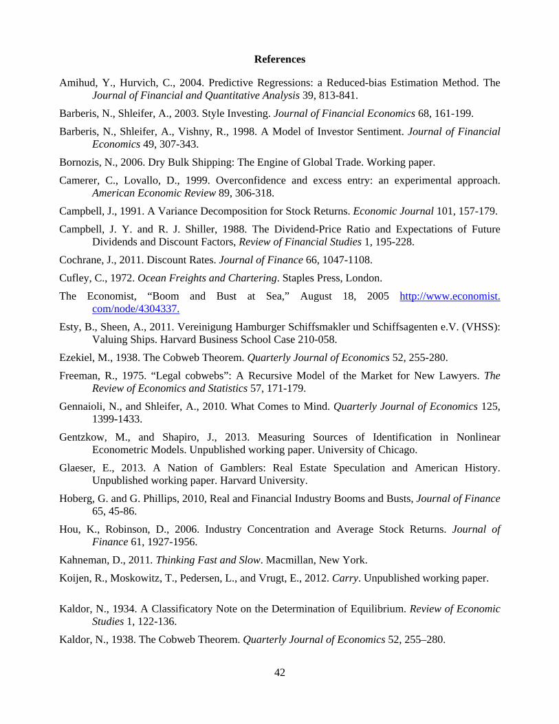
42

References

Amihud, Y., Hurvich, C., 2004. Predictive Regressions: a Reduced-bias Estimation Method. The Journal of Financial and Quantitative Analysis 39, 813-841.

Barberis, N., Shleifer, A., 2003. Style Investing. Journal of Financial Economics 68, 161-199.

Barberis, N., Shleifer, A., Vishny, R., 1998. A Model of Investor Sentiment. Journal of Financial Economics 49, 307-343.

Bornozis, N., 2006. Dry Bulk Shipping: The Engine of Global Trade. Working paper.

Camerer, C., Lovallo, D., 1999. Overconfidence and excess entry: an experimental approach. American Economic Review 89, 306-318.

Campbell, J., 1991. A Variance Decomposition for Stock Returns. Economic Journal 101, 157-179.

Campbell, J. Y. and R. J. Shiller, 1988. The Dividend-Price Ratio and Expectations of Future Dividends and Discount Factors, Review of Financial Studies 1, 195-228.

Cochrane, J., 2011. Discount Rates. Journal of Finance 66, 1047-1108.

Cufley, C., 1972. Ocean Freights and Chartering. Staples Press, London.

The Economist, “Boom and Bust at Sea,” August 18, 2005 http://www.economist. com/node/4304337.

Esty, B., Sheen, A., 2011. Vereinigung Hamburger Schiffsmakler und Schiffsagenten e.V. (VHSS): Valuing Ships. Harvard Business School Case 210-058.

Ezekiel, M., 1938. The Cobweb Theorem. Quarterly Journal of Economics 52, 255-280.

Freeman, R., 1975. “Legal cobwebs”: A Recursive Model of the Market for New Lawyers. The Review of Economics and Statistics 57, 171-179.

Gennaioli, N., and Shleifer, A., 2010. What Comes to Mind. Quarterly Journal of Economics 125, 1399-1433.

Gentzkow, M., and Shapiro, J., 2013. Measuring Sources of Identification in Nonlinear Econometric Models. Unpublished working paper. University of Chicago.

Glaeser, E., 2013. A Nation of Gamblers: Real Estate Speculation and American History. Unpublished working paper. Harvard University.

Hoberg, G. and G. Phillips, 2010, Real and Financial Industry Booms and Busts, Journal of Finance 65, 45-86.

Hou, K., Robinson, D., 2006. Industry Concentration and Average Stock Returns. Journal of Finance 61, 1927-1956.

Kahneman, D., 2011. Thinking Fast and Slow. Macmillan, New York.

Koijen, R., Moskowitz, T., Pedersen, L., and Vrugt, E., 2012. Carry. Unpublished working paper.

Kaldor, N., 1934. A Classificatory Note on the Determination of Equilibrium. Review of Economic

Studies 1, 122-136.

Kaldor, N., 1938. The Cobweb Theorem. Quarterly Journal of Economics 52, 255–280.

43

Kalouptsidi, M., 2013. Time to Build and Fluctuations in Bulk Shipping. American Economic Review, forthcoming.

Ljungqvist, L., and Sargent, T., 2004. Recursive Macroeconomic Theory, 2nd Edition. The MIT Press, Cambridge, MA.

McFadden, D., 1989. A Method of Simulated Moments for Estimation of Discrete Response Models without Numerical Integration. Econometrica 57, 995-1026.

Metaxas, B., 1971. The Economics of Tramp Shipping. Athlone Press, London.

Muth, J., 1961. Rational Expectations and the Theory of Price Movements. Econometrica 29, 315–335.

Nerlove, M., 1958. Adaptive Expectations and Cobweb Phenomena. Quarterly Journal of Economics 72, 227-240.

Newey, W., West, K., 1987. A Simple, Positive Semi-definite, Heteroskedasticity and Autocorrelation Consistent Covariance Matrix. Econometrica 55, 703-708.

Pakes, A., and Pollard, D., 1989. Simulation and the Asymptotics of Optimization Estimators. Econometrica 57, 1027-1057.

Rabin, M., 2002. Inference by Believers in the Law of Small Numbers. Quarterly Journal of Economics 117, 775-816.

Rosen, S., Murphy, K., Scheinkman, J., 1994. Cattle cycles. Journal of Political Economy 102, 468-492.

Shiller, R., 1981. Do Stock Prices Move too much to be Justified by Subsequent Changes in Dividends? American Economic Review 71, 421–436.

Stafford, E., Chao, A., Luchs, K., 2002. Ocean Carriers. Harvard Business School Case 202-027.

Stambaugh, R., 1999. Predictive Regressions. Journal of Financial Economics 54, 375-421.

Stopford, M., 2004. Shipping Strategies for the Future. Remarks at the Fortis Bank Christmas Seminar.

Stopford, M., 2009, Maritime Economics, 3rd Edition. Routledge, New York.

Tversky, A., Kahneman, D., 1974. Judgement under Uncertainty: Heuristics and Biases. Science 185, 1124-1131.

 

44  

Figure 1 The Dry Bulk Carrier Fleet

This figure illustrates the evolution of the dry bulk carrier fleet. Panel A shows t he composition the dry bulk carrier fleet from 1976 to 2011 in deadweight tonnes (DWT). Handysize ships carry 10,000 to 35,000 DWT, Handymax ships carry 35,000 to 59,000 DWT, Panamax ships carry 60,000 to 80,000 DWT, and Capesize ships carry more than 80,000 DWT. Panel B shows a simple measure of net realized investment—the 12-month percentage change in capacity—for the entire fleet as well as for Panamax ships.

Panel A. Fleet composition (in millions of DWT)

Panel B. Net realized investment (12-month percentage change in total capacity)

0

100

200

300

400

500

600

700

1976

1978

1980

1982

1984

1986

1988

1990

1992

1994

1996

1998

2000

2002

2004

2006

2008

2010

Cap

acit

y (M

illi

ons

of D

WT

)

Capesize Panamax Handymax Handysize

-5%

0%

5%

10%

15%

20%

25%

1976

1978

1980

1982

1984

1986

1988

1990

1992

1994

1996

1998

2000

2002

2004

2006

2008

2010

% C

han

ge in

Cap

acit

y

Panamax Fleetwide

 

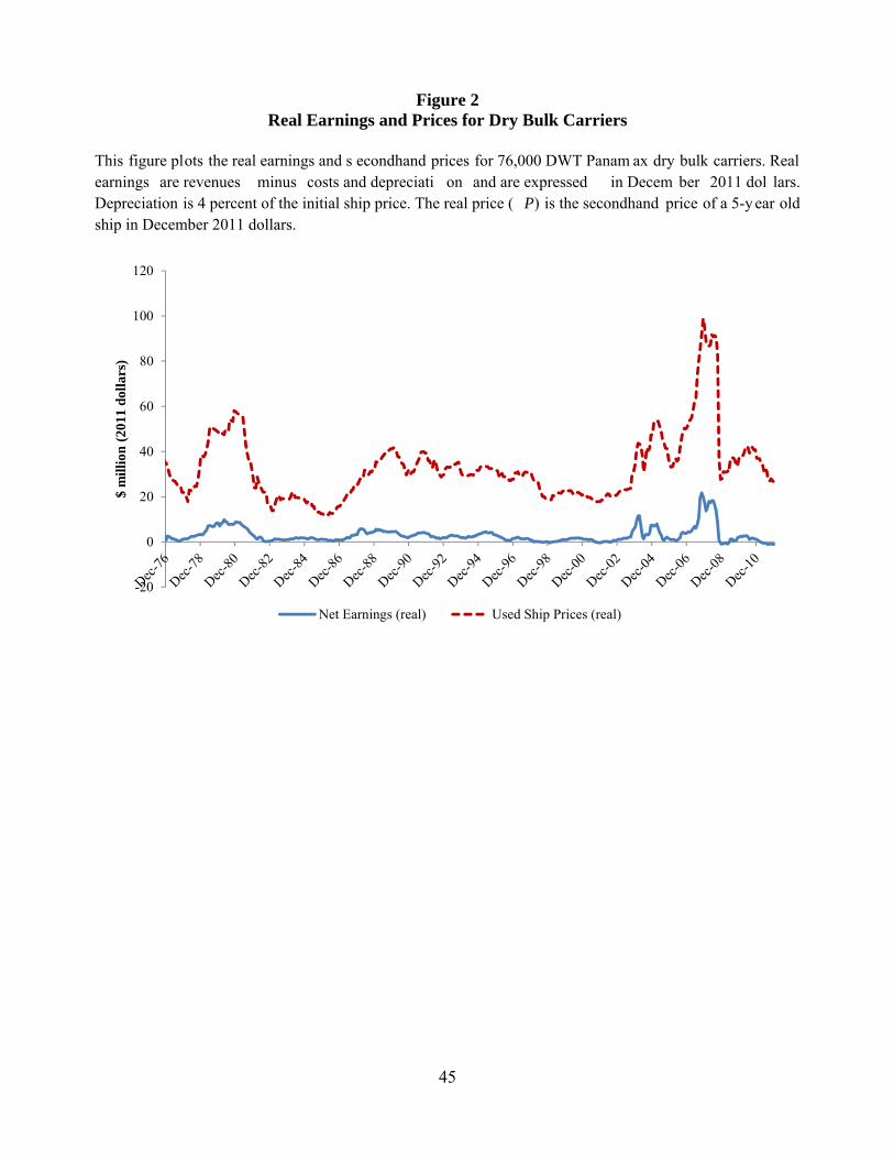
45  

Figure 2 Real Earnings and Prices for Dry Bulk Carriers

This figure plots the real earnings and s econdhand prices for 76,000 DWT Panam ax dry bulk carriers. Real earnings are revenues minus costs and depreciati on and are expressed in Decem ber 2011 dol lars. Depreciation is 4 percent of the initial ship price. The real price ( P) is the secondhand price of a 5-y ear old ship in December 2011 dollars.

-20

0

20

40

60

80

100

120

$ m

illio

n (2

011

dol

lars

)

Net Earnings (real) Used Ship Prices (real)

 

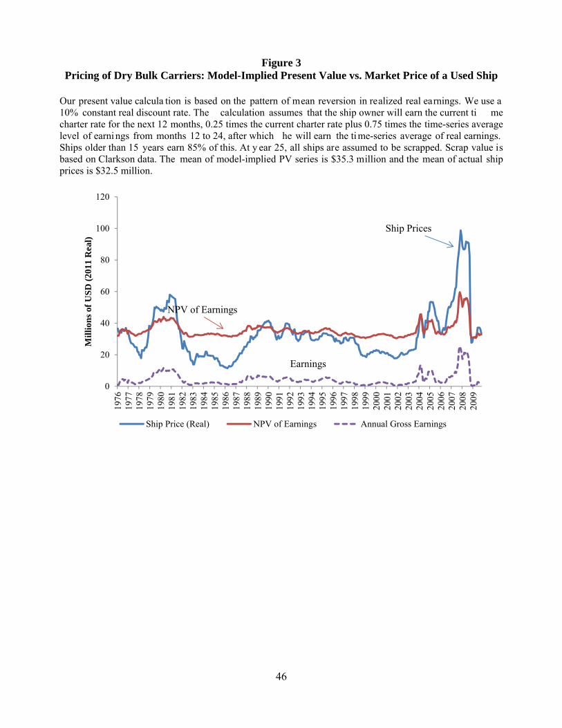
46  

Figure 3 Pricing of Dry Bulk Carriers: Model-Implied Present Value vs. Market Price of a Used Ship

Our present value calcula tion is based on the pattern of mean reversion in realized real earnings. We use a 10% constant real discount rate. The calculation assumes that the ship owner will earn the current ti me charter rate for the next 12 months, 0.25 times the current charter rate plus 0.75 times the time-series average level of earnings from months 12 to 24, after which he will earn the time-series average of real earnings. Ships older than 15 years earn 85% of this. At y ear 25, all ships are assumed to be scrapped. Scrap value is based on Clarkson data. The mean of model-implied PV series is $35.3 million and the mean of actual ship prices is $32.5 million.

0

20

40

60

80

100

120

1976

1977

1978

1979

1980

1981

1982

1983

1984

1985

1986

1987

1988

1989

1990

1991

1992

1993

1994

1995

1996

1997

1998

1999

2000

2001

2002

2003

2004

2005

2006

2007

2008

2009

Mil

lion

s of

US

D (

2011

Rea

l)

Ship Price (Real) NPV of Earnings Annual Gross Earnings

Earnings

NPV of Earnings

Ship Prices

 

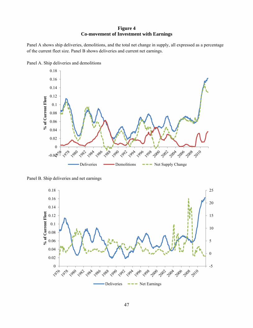
47  

Figure 4 Co-movement of Investment with Earnings

Panel A shows ship deliveries, demolitions, and the total net change in supply, all expressed as a percentage of the current fleet size. Panel B shows deliveries and current net earnings. Panel A. Ship deliveries and demolitions

Panel B. Ship deliveries and net earnings

-0.02

0

0.02

0.04

0.06

0.08

0.1

0.12

0.14

0.16

0.18

% o

f C

urr

ent

Fle

et

Deliveries Demolitions Net Supply Change

-5

0

5

10

15

20

25

0

0.02

0.04

0.06

0.08

0.1

0.12

0.14

0.16

0.18

% o

f C

urr

ent

Fle

et

Deliveries Net Earnings

 

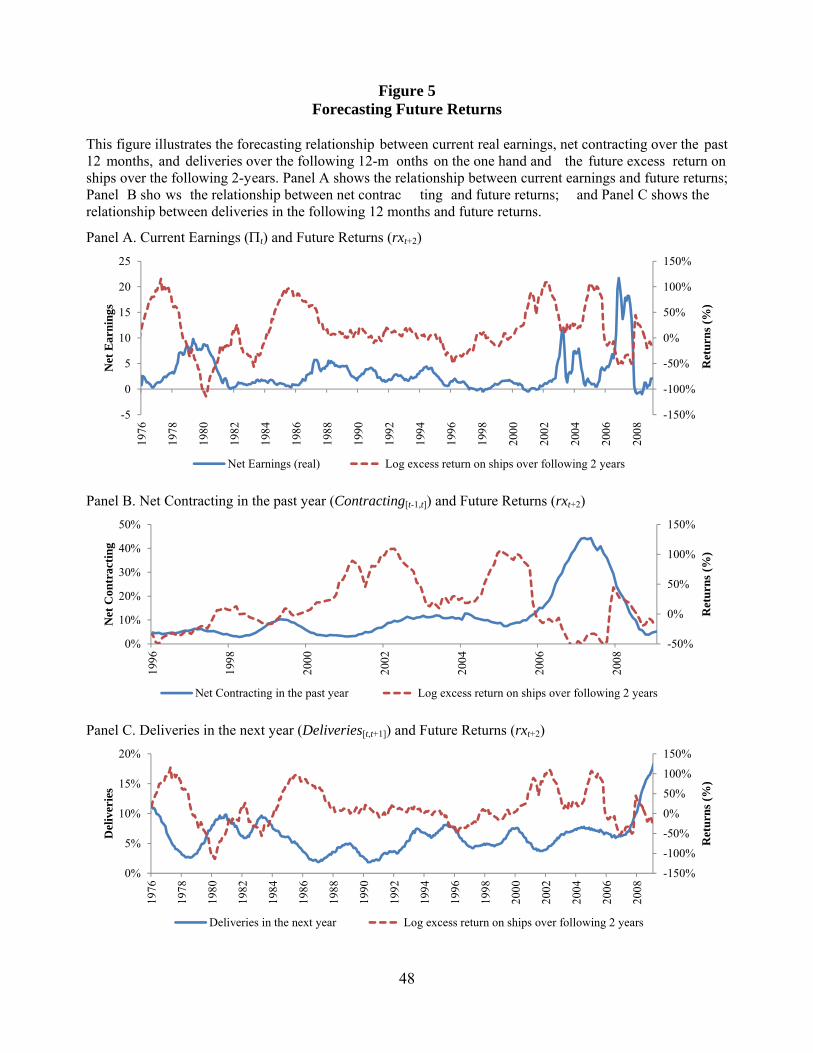
48  

Figure 5 Forecasting Future Returns

This figure illustrates the forecasting relationship between current real earnings, net contracting over the past 12 months, and deliveries over the following 12-m onths on the one hand and the future excess return on ships over the following 2-years. Panel A shows the relationship between current earnings and future returns; Panel B sho ws the relationship between net contrac ting and future returns; and Panel C shows the relationship between deliveries in the following 12 months and future returns.

Panel A. Current Earnings (t) and Future Returns (rxt+2)

Panel B. Net Contracting in the past year (Contracting[t-1,t]) and Future Returns (rxt+2)

Panel C. Deliveries in the next year (Deliveries[t,t+1]) and Future Returns (rxt+2)

 

-150%

-100%

-50%

0%

50%

100%

150%

-5

0

5

10

15

20

25

1976

1978

1980

1982

1984

1986

1988

1990

1992

1994

1996

1998

2000

2002

2004

2006

2008

Ret

urns

(%

)

Net

Ear

ning

s

Net Earnings (real) Log excess return on ships over following 2 years

-50%

0%

50%

100%

150%

0%

10%

20%

30%

40%

50%

1996

1998

2000

2002

2004

2006

2008

Ret

urn

s (%

)

Net

Con

trac

tin

g

Net Contracting in the past year Log excess return on ships over following 2 years

-150%

-100%

-50%

0%

50%

100%

150%

0%

5%

10%

15%

20%

1976

1978

1980

1982

1984

1986

1988

1990

1992

1994

1996

1998

2000

2002

2004

2006

2008

Ret

urns

(%

)

Del

iver

ies

Deliveries in the next year Log excess return on ships over following 2 years

 

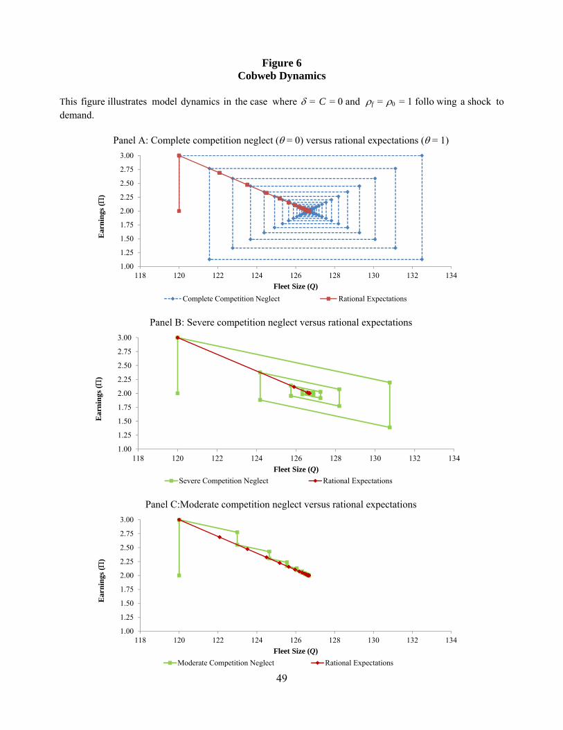
49  

Figure 6 Cobweb Dynamics

This figure illustrates model dynamics in the case where = C = 0 and f = = 1 follo wing a shock to demand.

Panel A: Complete competition neglect (= 0) versus rational expectations (= 1)

Panel B: Severe competition neglect versus rational expectations

Panel C:Moderate competition neglect versus rational expectations

1.00

1.25

1.50

1.75

2.00

2.25

2.50

2.75

3.00

118 120 122 124 126 128 130 132 134

Ear

nin

gs (

)

Fleet Size (Q)

Complete Competition Neglect Rational Expectations

1.00

1.25

1.50

1.75

2.00

2.25

2.50

2.75

3.00

118 120 122 124 126 128 130 132 134

Ear

nin

gs (

)

Fleet Size (Q)

Severe Competition Neglect Rational Expectations

1.00

1.25

1.50

1.75

2.00

2.25

2.50

2.75

3.00

118 120 122 124 126 128 130 132 134

Ear

nin

gs (

)

Fleet Size (Q)

Moderate Competition Neglect Rational Expectations

 

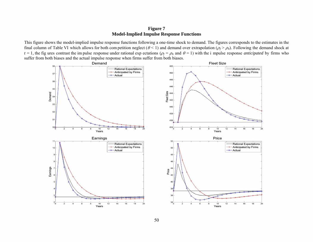
50  

Figure 7 Model-Implied Impulse Response Functions

This figure shows the model-implied impulse response functions following a one-time shock to demand. The figures corresponds to the estimates in the final column of Table VI which allows for both com petition neglect ( < 1) and demand over extrapolation (f > 0). Following the demand shock at t = 1, the fig ures contrast the im pulse response under rational exp ectations (f = 0 and = 1) with the i mpulse response anticipated by firms who suffer from both biases and the actual impulse response when firms suffer from both biases.

 

51  

Table I Summary Statistics

This table shows the mean, median, standard devi ation, extreme values, and one-m onth and 12-m onth autocorrelation coefficients for the main time-series data used in the paper. Panels A to D are based on time-series data on the dry bulk shipping industry provided by Clarkson. The sample is monthly and runs from January 1976 from December 2010, with the exception of order book data, which is only available beginning in January 1996. Panel A provides summary statistics for real ship earnings and real ship prices. Real earnings are revenues minus costs and expressed in December 2011 dollars. Also nominal figures are converted to Decem ber 2011 dollars using th e US Consu mer Price Index. Earnings ( ) are net of a depreciation expense, assumed to equal 4 percent of the initial ship price, while gross earnings do not account for depreciation. The real price (P) is the price of a 5-y ear old ship in December 2011 dollars. Panel B shows fleet dynamics. Deliveries[t,t+1] is deliveries over the following 1 2 months, Demolition[t-1,t] is demolitions over the past 12 months, and Invt = Deliveries[t,t+1] – Demolition[t-1,t]. Each of th ese variables is scaled by the time-t fleet size. Panel C summarizes order book dynamics. Specifically, Contracting[t-1,t] is net contracting (new contracting minus cancelations) over the past 12 months, and Orderst is the current size of the order book, both scaled by the time-t fleet size. Panel D summarizes the log excess returns on ships at a 1, 2, and 3-year horizon (rxt+k). The 1-year holding period return for a used ship is define d as net earnings over the 12-m onth period plus the capital gain from re selling the ship at the price in 12 months. Our measures of ship earnings, prices, and returns in Panels A and D are based on 76,000 DWT Panamax ships. However, fleet and order book dynamics data shown in Panels B and C are for the entire dr y bulk carrier fleet. Finally, Panel E summarizes several other time-series used in the paper: the annual log excess return on stocks (MKTRFt+1), the annual return on riskless government T-bills ( RFt+1), annual CPI inflation (CPI t+1), the dividend price yield for stocks (D/P), and the Shiller 10-year trailing earnings yield for stocks (E10/P). Variable N Mean Median SD Min Max ρ1 ρ12

Panel A: Annual Real Ship Earnings and Real Ship Prices (January 1976-December 2010) 420 2.99 1.87 3.40 -0.99 21.71 0.96 0.20 (gross) 420 4.30 3.10 3.94 0.23 25.38 0.96 0.24P 420 32.74 30.79 15.08 11.41 98.78 0.98 0.52/P 420 0.08 0.07 0.05 -0.03 0.27 0.94 0.22

Panel B: Fleet Dynamics (January 1976-December 2010) Deliveries[t,t+1] 420 0.065 0.062 0.034 0.018 0.186 1.01 0.81Demolition[t-1,t] 420 0.017 0.013 0.014 0.001 0.063 0.99 0.66Invt 420 0.048 0.047 0.039 -0.031 0.175 1.00 0.77

Panel C: Order Book Dynamics (January 1996-December 2010) Contracting[t-1,t] 169 0.114 0.090 0.101 0.029 0.443 0.99 0.39Orderst 180 0.269 0.147 0.230 0.072 0.789 1.00 0.96

Panel D: Ship Excess Returns (Various date ranges) rxt+1 420 0.063 0.058 0.316 -0.756 0.858 0.96 0.03rxt+2 408 0.141 0.079 0.454 -1.141 1.155 0.98 0.43rxt+3 396 0.219 0.144 0.534 -0.876 1.429 0.99 0.70

Panel E: Other Variables (January 1976-December 2010) MKTRFt+1 420 0.051 0.074 0.163 -0.567 0.423 0.93 -0.05RFt+1 420 0.053 0.051 0.031 0.000 0.142 1.00 0.90CPI t+1 420 0.039 0.032 0.027 -0.021 0.138 0.99 0.74D/P (stocks) 420 0.029 0.027 0.013 0.010 0.057 0.98 0.95E10/P (stocks) 420 0.063 0.051 0.031 0.023 0.151 1.00 0.93

 

52  

Table II Forecasting Ship Returns Using Ship Earnings and Prices

Table II reports time-series forecasting regressions of the form

t k t t krx a b X c t u , where rxt+k denotes the k-period log excess r eturn on a ships. Xt alternately denotes real e arnings t, the current real price of a 5-year used ship Pt, or the earnings yield t/Pt. The k-year forecasting regressions are estimated with monthly data, so we are forecasting excess returns over the following 12× k months. To deal with the overlapping nature of returns, t-statistics are based on Newey-West (1987) standard errors allowing for serial correlation at up to 1.5 ×12× k monthly lags—i.e., we allow for serial correlation at up 18, 36, and 54 month lags, respectively, when forecasting 1-, 2-, and 3-year returns. X = Real Earnings X = Used Ship Price P X = Earnings Yield /P

k: 1-yr 2-yr 3-yr 1-yr 2-yr 3-yr 1-yr 2-yr 3-yr Panel A. Univariate

b -0.026 -0.049 -0.061 -0.007 -0.013 -0.016 -0.557 -1.990 -2.670[t] [-2.49] [-3.38] [-2.63] [-2.69] [-3.11] [-2.82] [-0.65] [-1.63] [-1.67]T 420 408 396 420 408 396 420 408 396R2 0.08 0.14 0.16 0.12 0.19 0.22 0.01 0.05 0.07

Panel B. Including a time trend b -0.026 -0.050 -0.063 -0.008 -0.014 -0.018 -0.527 -1.961 -2.638[t] [-2.40] [-3.49] [-2.85] [-2.98] [-3.81] [-3.64] [-0.58] [-1.67] [-1.68]c 0.016 0.036 0.052 0.039 0.073 0.094 0.007 0.008 0.013[t] [0.35] [0.45] [0.50] [0.82] [0.86] [0.84] [0.14] [0.09] [0.12]T 420 408 396 420 408 396 420 408 396R2 0.08 0.15 0.17 0.14 0.22 0.26 0.01 0.05 0.07

 

53  

Table III Investment and Future Returns

Table III reports time-series forecasting regressions of the form

t k t t krx a b X c t u , where rxt+k denotes the k-year log holding period excess return on a Panamax dry bulk ship. X alternately denotes net contracting activity over the past 12 months, the size of the order book, deliveries over the follo wing 12 months, or demolitions over the past 12 months, each scaled by the current fleet size. In the rightmost set of columns, we forecast returns using net investment, Inv[t-1,t] = Deliveries[t,t+1] – Demolitions[t-1,t]. The k-year forecasting regressions are estimated with monthly data, so we are forecasting excess retu rns over the following 12× k months. To deal with the overlapping nature of returns, t-statistics are based on Newey -West (1987) standard errors allowing for serial correlation at up to 1.5 ×12× k monthly lags—i.e., we allow for serial correlation at up 18, 36, and 54 month lags, respectively, when forecasting 1-, 2-, and 3-year returns.

Investment Measured Based on Order Book (1996-2010) Investment Measured Based on Changes in Fleet Size (1976-2010) X = Contracting[t-1,t] X = Orderst X = Deliveries[t,t+1] X = Demolition[t-1,t] X = Inv[t-1,t]

k: 1-yr 2-yr 3-yr 1-yr 2-yr 3-yr 1-yr 2-yr 3-yr 1-yr 2-yr 3-yr 1-yr 2-yr 3-yr Panel A. Univariate

b -1.105 -1.503 -2.132 -0.344 -0.520 -1.065 -3.055 -5.038 -2.043 5.475 9.347 12.971 -2.986 -5.071 -3.931 [t] [-2.09] [-2.07] [-2.28] [-1.30] [-1.34] [-1.84] [-2.41] [-2.35] [-0.55] [1.82] [1.62] [1.75] [-2.99] [-2.39] [-1.08] T 169 157 145 180 168 156 420 408 396 420 408 396 420 408 396 R2 0.11 0.12 0.20 0.06 0.07 0.14 0.11 0.09 0.01 0.06 0.09 0.13 0.14 0.14 0.05

Panel B. Including a time trend b -1.750 -3.006 -5.270 -1.353 -2.253 -3.319 -3.340 -5.161 -1.934 5.469 9.309 13.001 -3.186 -5.137 -3.885 [t] [-2.66] [-2.50] [-3.80] [-2.85] [-4.72] [-4.83] [-2.81] [-2.35] [-0.54] [-1.80] [-1.60] [-1.70] [-3.32] [-2.31] [-1.07] c 0.249 0.558 1.096 0.539 0.982 1.210 0.033 0.033 0.023 0.011 0.020 0.029 0.032 0.032 0.020 [t] [1.27] [1.53] [2.59] [2.76] [5.26] [4.09] [0.76] [0.40] [0.20] [0.23] [0.24] [0.24] [0.74] [0.38] [0.17] T 169 157 145 180 168 156 420 408 396 420 408 396 420 408 396 R2 0.20 0.32 0.59 0.29 0.49 0.65 0.12 0.10 0.01 0.06 0.09 0.13 0.15 0.15 0.05

 

54  

Table IV Bivariate Forecasting Regressions

Table IV reports time-series regressions of the form

[ 1, ]t k t t t t krx a b c Inv d t u , where rxt+k denotes the k-year log holding period excess ret urn on a Pana max dry bulk ship, and the independent variables include net earnings and investment. Investment Inv[t–1,t] is defined as deliveries minus demolitions as in the rightmost columns of Table III. The last three columns also include a time trend. The k-year forecasting regressions are estimated with monthly data, so we ar e forecasting excess returns over the following 12× k months. To deal with the overlapping nature of returns, t-statistics are based on Newey-West (1987) standard errors allowing for serial correlation at up to 1.5 ×12× k monthly lags—i.e., we allow for serial correlation at up 18, 36, and 54 month lags, respectively, when forecasting 1-, 2-, and 3-year returns.

Return Forecasting Horizon: k: 1-yr 2-yr 3-yr 1-yr 2-yr 3-yr

b -0.023 -0.043 -0.056 -0.023 -0.044 -0.058[t] [-2.24] [-3.19] [-2.37] [-2.08] [-3.34] [-2.59]c -2.811 -4.455 -2.645 -3.027 -4.527 -2.484[t] [-3.01] [-2.18] [-0.76] [-3.35] [-2.14] [-0.70]d 0.035 0.042 0.046[t] [0.84] [0.51] [0.43]T 420 408 396 420 408 396R2 0.20 0.25 0.18 0.21 0.26 0.19

 

55  

Table V Equity Risk Premium Controls

Table VI repeats the time-series return forecasting regressions from Table III and Table IV adding ex-ante and ex-post measures of risk premia from the US equity market. The time-series regressions take the form

2 2t t t trx a b X c Z u , and

2 , 2 , 2 , 2 , 2 2t t t t t t t t t t trx a b X c M KTRF d HM L e SM B f M OM u where rxt+k denotes the 2 -year (log) holding period excess return on a Panamax dry bulk ship, and Xt is alternately ship earnings, used prices, or ne t investment, defined as deliveries minus demolitions as in the rightmost columns of Table III. In Panel A, Zt denotes ex-ante risk premium measures, including the dividend-price ratio, the earnings-price ratio, and the risk-free rate. In Panel B, the control variables include ex-post risk factor realizations, including the 24-month excess realized return on the s tock market (MKTRF) and the 24-month cumulative returns on the value (HML), size (SMB), and momentum (MOM) factors. t-statistics are based on Newey West (1987) standard errors with 36 months of lags. Panel A. Ex-ante risk premium controls Dependent Variable: 2-year excess return on Panamax Ship

Equity premium forecasters only

Horse race regressions

ship) -0.048 -0.049 -0.044 [-3.66] [-3.65] [-4.04] Pship) -0.013 -0.013 -0.013 [-3.49] [-3.44] [-4.47]Invship) -4.981 -4.987 -5.139 [-2.44] [-2.58] [-2.78]D/P (stocks) -3.877 -2.878 -4.936 -2.782 [-0.53] [-0.39] [-0.65] [-0.40]E10/P (stocks) -1.546 -1.269 -2.077 -0.423 [-0.51] [-0.41] [-0.64] [-0.15]Risk-free rate -62.816 -56.148 -65.107 -63.741

[-2.42] [-2.42] [-3.20] [-4.06]T 408 408 408 408 408 408 408 408 408 408 408 408R2 0.01 0.01 0.13 0.15 0.15 0.24 0.21 0.21 0.33 0.15 0.14 0.28

 

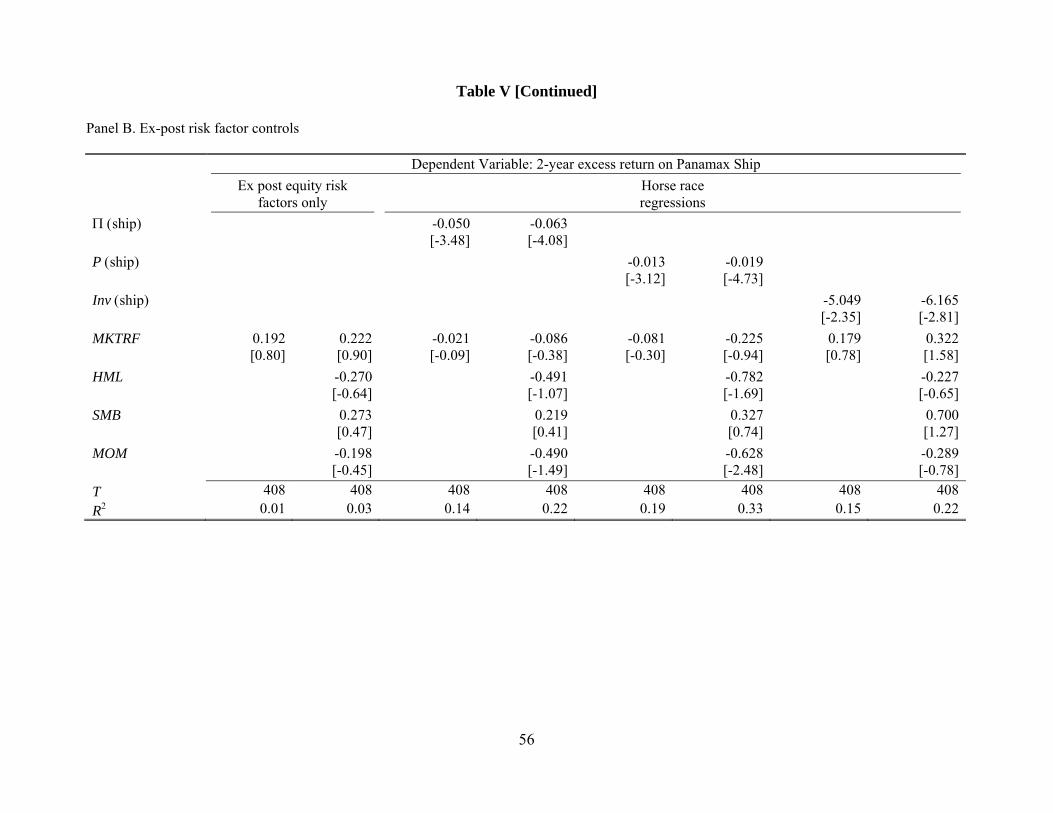
56  

Table V [Continued] Panel B. Ex-post risk factor controls Dependent Variable: 2-year excess return on Panamax Ship

Ex post equity risk

factors only Horse race regressions

ship) -0.050 -0.063 [-3.48] [-4.08]Pship) -0.013 -0.019

[-3.12] [-4.73]Invship) -5.049 -6.165

[-2.35] [-2.81]MKTRF 0.192 0.222 -0.021 -0.086 -0.081 -0.225 0.179 0.322

[0.80] [0.90] [-0.09] [-0.38] [-0.30] [-0.94] [0.78] [1.58]HML -0.270 -0.491 -0.782 -0.227

[-0.64] [-1.07] [-1.69] [-0.65]SMB 0.273 0.219 0.327 0.700

[0.47] [0.41] [0.74] [1.27]MOM -0.198 -0.490 -0.628 -0.289

[-0.45] [-1.49] [-2.48] [-0.78]T 408 408 408 408 408 408 408 408R2 0.01 0.03 0.14 0.22 0.19 0.33 0.15 0.22

 

57  

Table VI Simulated Method of Moments Estimation of the Structural Model

We match M = 22 simulated moments to moments from our data to estimate L = 7 parameters in the model. We generate a sim ulated 100,000 year time-series using the model and fi nd the m odel parameters that minimize the sum of the squared differences bet ween simulated and e mpirical moments, weighting each moment inversely to its estimated variance. We estimate the covariance matrix of the sample moments using a Newey-West (1987) style estimator for seemingly-unrelated-regression.

Simulation Values Empirical Rational Imposing f= Imposing = 1 Unrestricted Values Expectations Only Only Expectations

Moment m [t] m m m m

1 E[rxt+1] 0.079 [1.49] 0.075 0.091 0.068 0.068 2 Var[rxt+1] 0.101 [4.59] 0.046 0.060 0.059 0.084 3 E[t] 3.058 [4.87] 2.916 2.983 2.739 2.768 4 Var[t] 12.126 [1.97] 21.455 21.558 22.030 17.670 5 E[Pt] 32.448 [8.90] 30.762 27.209 32.049 37.328 6 Var[Pt] 238.683 [2.14] 7.016 6.473 13.728 51.311 7 Corr[t,t+1/12] 0.960 [47.58] 0.943 0.935 0.942 0.968 8 Corr[t,t+1] 0.197 [1.31] 0.449 0.406 0.422 0.533 9 Corr[t,t+2] -0.096 [-1.02] 0.183 0.148 0.150 0.255 10 (rxt+1|t) -0.027 [-3.05] 0.000 -0.003 -0.007 -0.019 11 (rxt+2|t) -0.051 [-3.28] 0.000 -0.004 -0.010 -0.030 12 (rxt+1|Pt) -0.007 [-3.12] 0.000 -0.006 -0.007 -0.010 13 (rxt+2|Pt) -0.013 [-3.06] 0.001 -0.008 -0.011 -0.017 14 (rxt+1|t/Pt) -0.737 [-0.82] 0.004 -0.082 -0.214 -0.721 15 (rxt+2|t/Pt) -2.160 [-1.69] 0.001 -0.103 -0.344 -1.134 16 (rxt+1|It/Qt) -3.314 [-2.10] 0.299 -3.992 -4.194 -6.026 17 (rxt+2|It/Qt) -5.053 [-1.99] 0.397 -5.476 -6.662 -9.673 18 (It/Qt|Pt) 0.001 [5.31] 0.002 0.001 0.002 0.002 19 (rxt+1|It/Qt,t) -2.881 [-1.73] 1.096 -3.257 2.606 -0.571 20 (rxt+1|It/Qt,t) -0.023 [-2.14] -0.001 -0.001 -0.010 -0.018 21 (rxt+2|It/Qt,t) -4.213 [-1.70] 2.233 -6.447 4.621 -1.558 22 (rxt+2|It/Qt,t) -0.044 [-3.14] -0.002 0.001 -0.016 -0.026

GMM Criterion Function J = 106.90 J = 59.90 J = 67.55 J = 45.86

Corresponding Parameter Estimates: b [t] b [t] b [t] b [t] N/A N/A 0.459 [3.91] N/A N/A 0.500 [3.82] f N/A N/A N/A N/A 0.600 [8.92] 0.797 [19.20] 0 0.493 [6.09] 0.445 [6.32] 0.488 [8.69] 0.676 [15.52] 4.147 [4.95] 4.255 [5.09] 4.259 [6.03] 3.559 [5.81] k 1.524 [5.50] 1.565 [6.28] 1.350 [7.35] 1.343 [8.76] r 0.095 [6.56] 0.110 [6.29] 0.086 [7.32] 0.074 [7.60] Pr 30.762 [10.36] 27.209 [8.90] 32.049 [8.07] 37.327 [7.44]

Hypothesis Tests on Estimated Parameters: N/A t = 4.60 N/A t = 3.82

f N/A N/A t = 2.91 t = 3.30