Wavelet Frame Based Blind Image Inpainting

Bin Dongb,, Hui Jia,∗, Jia Lia, Zuowei Shena, Yuhong Xuc

aDepartment of Mathematics, National University of Singapore, Singapore, 117542bDepartment of Mathematics, University of California, San Diego, 9500 Gilman Drive, La

Jolla, CA, 92093-0112cCenter for Wavelets, Approx. and Info. Proc., National University of Singapore,

Singapore, 117542

Abstract

Image inpainting has been widely used in practice to repair damaged/missingpixels of given images. Most of the existing inpainting techniques require know-ing beforehand where those damaged pixels are, either given as a priori ordetected by some pre-processing. However, in certain applications, such in-formation neither is available nor can be reliably pre-detected, e.g. removingrandom-valued impulse noise from images or removing certain scratches fromarchived photographs. This paper introduces a blind inpainting model to solvethis type of problems, i.e., a model of simultaneously identifying and recov-ering damaged pixels of the given image. A tight frame based regularizationapproach is developed in this paper for such blind inpainting problems, andthe resulted minimization problem is solved by the split Bregman algorithmfirst proposed by [1]. The proposed blind inpainting method is applied to var-ious challenging image restoration tasks, including recovering images that areblurry and damaged by scratches and removing image noise mixed with bothGaussian and random-valued impulse noise. The experiments show that ourmethod is compared favorably against many available two-staged methods inthese applications.

Key words: image inpainting, sparse approximation, split Bregmanalgorithm, wavelet frame

1. Introduction

The word “inpainting” has been used by museum restoration artists for quitea while before the concept was applied to digital image inpainting first by [2].Image inpainting problem occurs when image pixels are missing, over-writtenor damaged by some other means. This arises for example in restoring ancient

∗Corresponding author. Tel.: +65-65168845, Fax: +65-67795452Email addresses: dongbin725@gmail.com (Bin Dong), matjh@nus.edu.sg (Hui Ji),

lijia@nus.edu.sg (Jia Li), matzuows@nus.edu.sg (Zuowei Shen), tslxyh@nus.edu.sg(Yuhong Xu)

Preprint submitted to Elsevier May 15, 2011

drawings or old videos where a portion of a picture or frame is missing ordamaged due to aging or scratching; or when an image is corrupted by impulsenoise due to noisy sensors or channel transmission error. Thus, image inpaintingis about recovering the missing information within the damaged regions from theincomplete and noisy observation of the image. An ideal recovery of an imagein the corrupted regions should possess image features, like edges and textures,that are consistent to the features observed. In recent years, there have beengreat progresses on image inpainting, see [2, 3, 4, 5, 6, 7, 8, 9, 10, 11, 12, 13, 14]and the references therein.

The model for general image inpainting problem, accompanied by other im-age degradation effects such as blurring, can be formulated as follows. Let animage be represented as a column vector in Rn, where n is the total numberof pixels. Then the mathematical formulation of imaging inpainting can beexpressed as

f(i)=

{(Hu)(i)+ϵ(i), i∈Λv(i), i∈Λc,

(1.1)

where f is the observed corrupted image, u is the original image that we aretrying to recover, ϵ represents i.i.d. additive Gaussian white noise ([15]), H issome degradation operator (e.g. convolution for image blurring), and Λ is theindex set of certain pixels of the image. The random-valued vector v repre-sents the values of all other image pixels corrupted by other factors (besidesGaussian white noise). The sub-vector v|Λc of v defined on Λc can representvarious types of degradations to the original image, including impulse noise (e.g.salt-and-pepper noise and random-valued impulse noise) and random-patternedscratching with unknown intensities. The goal of image inpainting is then toestimate the original image u from the observation f .

The index set Λc is called the inpainting region/domain which is assumedto be known or estimated beforehand in most literatures. However, in someapplications, the inpainting domain may not be readily available, or it can notbe accurately detected by some separate process, e.g. when the vector v in(1.1) contains random-valued impulse noise mixed with Gaussian white noise.We call such a inpainting problem a blind inpainting problem, that is, both theinpainting domain Λc (or equivalently the projection PΛ) and the original imageu are unknown. In contrast to regular image inpainting problems in which Λis known, both Λ and u are unknown in blind inpainting problem. Thus, blindinpainting problem is a highly ill-posed inverse problem.

In recent years, there have been a few works on solving such blind inpaintingproblems. For video restoration, the blind inpainting problem is first discussedin [16]. Based on the same sparsity prior of damaged pixels in image space, apatch-based approach is proposed in [16] to do blind video inpainting. For imagerestoration, the blind inpainting problem for repairing damaged pixels is tackledby [17] and [18], both of which use the ℓ1 norm as the fidelity measurement tosuppress the outlier effect of damaged pixels. The differences between them isone is using non-local total variation (TV) regularization ([17]) and the other isusing ℓ1 norm of tight frame coefficients ([18]). Recently, a TV-based approach

2

is proposed [19] to simultaneously identify occlusions and estimating optical flowof a video sequence, which also can be viewed as a blind inpainting problem.

The goal of this paper is to develop computational models and correspond-ing efficient algorithms for solving such blind image inpainting problems. Inthis paper, we take a Lagrangian regularization approach to tackle such an ill-posed inverse problem. In order to overcome the ill-posedness of the problem,appropriate regularization terms on both the original image u and the inpaint-ing region Λc have to be enforced in the minimization model. The basic ideaof our approach is to utilize the sparsity priors of images and random-valuedvector v in different domains. Motivated by the impressive performance of usingsparsity prior of images under tight wavelet frames in many image restorationtasks ([20, 21, 22, 23, 24, 25, 26, 27, 11, 12, 13]), we also use the ℓ1 norm ofwavelet tight frame coefficients of images as the regularization term for imagesin our approach. Since the values of v|Λ can be arbitrary, we seek the solutionto v whose elements defined on the index Λ are zeros. Since the number of theinpainting domain Λc is usually much less than that of the whole image domain,we assume that v is sparse in spatial domain. Such an assumption is utilized inour approach by using the ℓ1 norm of v in spatial domain as the regularizationterm on v. Moreover, the ℓ1 related minimization resulting from our proposedmodels can be efficient solved using the so-called split Bregman method. Thesplit Bregman iteration is first proposed in [1] with many successful applicationsin imaging sciences (see e.g. [1, 28, 29]).

The rest of this paper will be organized as follows. In Section 2, we willpropose two sparsity-based regularization models for blind image inpainting.In Section 3, the split Bregman iteration based algorithms will be applied tosolve the minimization problems resulted from the proposed models. Numericalexperiments will be conducted in Section 4 for three image restoration tasks:

1. image denoising for random-valued impluse noise mixed with Gaussiannoise.

2. image deblurring in the presence of both random-valued impulse noise andGaussian white noise.

3. blind image inpainting for images corrupted by multiple sources includingrandom-valued impulse noise, Gaussian white noise and scratching.

2. Frame Based Blind Inpainting Models

Before presenting our regularization models for blind image inpainting, webriefly review a few facts of discrete tight wavelet frame decomposition and re-construction. Interesting readers should consult [30, 31, 32] for theories of framesand framelets, [12] for a short survey on theory and applications of frames, and[13] for a more detailed survey. In the discrete setting, a 2-dimensional imageis a 2-dimensional array that can be understood as a vector living in Rn, withn the total number of pixels in the image. Then the discrete framelet decom-position and reconstruction can be represented as matrix multiplications Wu

3

and W⊤v respectively. Here W ∈Rk×n satisfies W⊤W = I, i.e. u=W⊤Wu,∀u∈Rn, where W is derived by the filters of framelets obtained by the unitaryextension principle [31]. The matrix multiplications by W and W⊤v are onlyfor the notational convenience. In our numerical implementations, these twomatrix multiplications are done by using the fast tensor product tight waveletframe decomposition and reconstruction algorithms instead, which are essen-tially just the convolution of images by a set of filters. Interested readers canrefer to [13, 27] for more details.

2.1. Blind Inpainting Model: Single System

For notational convenience, we denote the projection matrix PΛ associatedto each Λ as an n×n diagonal matrix with the diagonal entries 1 for the indicesin Λ and 0 otherwise. Under this notation, (1.1) can be written equivalently as

PΛf =PΛ(Hu+ϵ) and PΛcf =PΛcv. (2.1)

We propose the following model to solve the blind image inpainting problem(2.1)

minu,v

1

2∥Hu+v−f∥22+λ1∥Wu∥1+λ2∥v∥1, (2.2)

where u is the ideal image that we are trying to recover, v is the random-valued vector in the observed image f , H is some degradation matrix, and W isthe decomposition matrix associated to some tight framelet system. The basicidea of (2.2) is as follows. Besides the variable u that represents the unknowntrue image, we introduce a new variable v in the fidelity term. The role of thisvariable is to explicitly represents the outliers (pixels damaged by impulse noise)existing in f . Certain regularizations on both variables u and v are needed tosolve the ill-posed linear system Hu+v=f . The proposed regularization on thetrue image u is based on the assumption that a clear noise-free image u shouldhave a sparse approximation under wavelet tight frame domain. The proposedregularization on the variable v is based on the assumption that the percentageof pixels damaged by impulse noise is small, which is equivalent to say thatthe vector v is sparse with only a small percentage of non-zero elements. Asa convex relaxation of ℓ0-norm that measures the exact sparsity of the signal,ℓ1-norm is used on both Wu and v in (2.2) to measure their sparsities. For thecase H is the identity, a similar model already appeared in [17] with non-localtotal variation (TV) regularization.

In our proposed approach, the vector v is explicitly defined as an unknown tobe estimated in the optimization model. There are a few alternative approachesto handle the random-valued vector v. One of them appears in [11, 18] is thetwo-stage approach that estimates the inpainting region Λ before estimating u.Then the problem (2.1) is reduced to a regular inpainting problem:

minu

1

2∥PΛ(Hu−f)∥22+λ∥Wu∥1. (2.3)

Such a two-stage approach works well when an accurate detection of Λ is pos-sible, e.g. detecting salt-and-pepper noise using adaptive median filter ([33]).

4

However, it is much harder to accurately detect general random-valued impulsenoise in images. Such unavoidable detection errors of Λ could seriously hamperthe performance of the inpainting if using (2.3), as we will see in our experi-ments.

The other approach is first proposed by [18, 34, 35] that treats v as theoutliers and uses the ℓ1 norm in the fidelity term to increase the robustness ofinpainting to outliers:

minu

∥Hu−f∥1+λ∥Wu∥1. (2.4)

This model can also be applied to the blind image inpainting problems. Whenthere exists only random-valued impulsive noise, the performance of the reg-ularization model (2.4) is similar to the proposed model (2.2) as we observedin the experiments. In practice, however, image noise is hardly from a singlesource. Five major sources of image noise with different statistical distributionshave been identified in [36] including amplifier noise modeled by Gaussian noise.In the presence of noises from multiple sources such as the mixture of impulsenoise and Gaussian noise, the model (2.2) is better than (2.4). The reason isas follows. It is known that the ℓ2 norm based fidelity term yields the optimalestimate in the presence of only Gaussian noise. Although the ℓ1 norm basedfidelity term used in (2.4) suppresses the negative impact caused by the out-liers, the adverse effect is the less optimal usage of the other data polluted bymostly Gaussian noise. On the contrary, the proposed model (2.2) uses thosedata damaged by mostly Gaussian noise in an optimal way while avoiding theoutlier effect of other data. The experimental evaluation in Section 4 will alsojustify the advantage of the regularization (2.2) over (2.4).

2.2. Blind Inpainting Model: Two Systems

The success of the model (2.2) largely relies on the validity of two sparsityassumptions: one is the sparsity of images in wavelet tight frame domain and thesparsity of v in image domain. Thus, the model (2.2) is suitable for images thatare piecewise smooth. When there exists rich texture information in images,these texture features are no longer piecewise smooth and they are relativelysparse in image domain ([37, 38, 39]). As a result, it is possible in (2.2) thatthese texture features are wrongly identified as the elements of v instead ofbeing preserved in u. Thus, the model (2.2) needs to be modified to prevent thetexture features from being absorbed into the vector v.

Our proposed approach is based on the observation that many types oftextures can be sparsely approximated by local discrete cosine transform (localDCT), which has been successfully used in some image restoration tasks ([25,10, 22]). Motivated by these approaches, we propose the following model forblind inpainting problem:

minu1,u2,v

1

2∥H(u1+u2)+v−f∥22+λ1∥Wu1∥1+λ2∥v∥1+λ3∥Du2∥1. (2.5)

5

Here D represents the local DCT, u1 is the cartoon component and u2 is thetexture component, and the desired recovery u=u1+u2. The model (2.5) pro-vided a more accurate estimate of u than (2.2) does for images of rich textureinformation. However, the complexity of the resulting minimization problem isalso increased, which leads to a higher computational cost. Thus, both modelshave their own merits and the choice of using either one of them should dependson the image content. The model (2.2) is more suitable for images without richtextures and the model (2.5) is more suitable for images with rich textures.

3. Numerical Algorithms

In this section, we will present numerical algorithms that solves our pro-posed models (2.2) and (2.5), as well as (2.4) and (2.3) used for experimentalevaluation. All of these algorithms are built upon the split Bregman iteration.The split Bregman algorithm was first proposed in [1] which showed its effi-ciency applied to various PDE based image restoration models , e.g., ROF andnonlocal variational models ([1, 40]). Convergence analysis of the split Breg-man algorithm, as well as its applications in various wavelet frame based imagerestoration algorithms, were given in [22]. For the completeness, we give a briefintroduction of the basic idea of split Bregman algorithm. Interesting readersare referred to [1, 22] for more details.

Consider the following minimization problem

minu

E(u)+λ∥Lu∥1, (3.1)

where E(u) is a smooth convex functional and L is some linear operator. Letd=Lu. Then (3.1) can be rewritten as

minu,d=Lu

E(u)+λ∥d∥1. (3.2)

Note that both u and d are variables now. The derivation of splitting Bregmaniteration for solving (3.2) is based on Bregman distance ([1, 22]). It was recentlyshown (see e.g. [41, 42]) that the split Bregman algorithm can also be derived byapplying augmented Lagrangian method (see e.g. [43]) to (3.2). The connectionbetween split Bregman algorithm and Douglas-Rachford splitting was addressedby [44]. We shall skip the detailed derivations and directly describe the splitBregman algorithm that solves (3.1) through (3.2) as follows,

uk+1=argminuE(u)+ µ2 ∥Lu−dk+bk∥22,

dk+1=argmindλ∥d∥1+ µ2 ∥d−Luk+1−bk∥22,

bk+1= bk+Luk+1−dk+1.

(3.3)

By [45, 46], the second subproblem has a simple analytical solution based onsoft-thresholding operator. Therefore, (3.3) can be written equivalently as

uk+1=argminuE(u)+ µ2 ∥Lu−dk+bk∥22,

dk+1=Tλ/µ(Luk+1+bk),

bk+1= bk+(Luk+1−dk+1),

(3.4)

6

where Tθ is the soft-thresholding operator defined by

Tθ :x=[x1,x2, ··· ,xM ]→Tθ(x)= [tθ1(x1),tθ2(x2), ··· ,tθM (xM )],

withtθi(xi)=sgn(xi)max{0, |xi|−θi}.

Note that the last two steps of (3.4) are straightforward and very efficient tocompute, while the computation cost of the first step is usually more expensiveas it involves the procedure of solving some linear system.

3.1. Algorithms Solving Our Models (2.2) and (2.5)

The minimization (2.2) can be efficiently solved split Bregman iteration. Letd=Wu and rewrite (2.2) as

minu,v,d=Wu

1

2∥Hu+v−f∥22+λ1∥d∥1+λ2∥v∥1.

Then we have the following iterative schemes that solves the above optimizationproblem:

uk+1=argminu12∥Hu+vk−f∥22+

µ2 ∥Wu−dk+bk∥22,

vk+1=argminvλ2∥v∥1+ 12∥v−(f−Huk+1)∥22,

dk+1=argmindλ1∥d∥1+ µ2 ∥d−(Wuk+1+bk)∥22,

bk+1= bk+(Wuk+1−dk+1).

The complete description of the algorithm for solving (2.2) is provided in Algo-rithm 1.

Algorithm 1 Numerical algorithm for solving (2.2)

(i) Set initial guesses u0, v0, d0, b0. Choose an appropriate set of parameters(λ1,λ2,µ).

(ii) For k=0,1,..., perform the following iterations until convergenceuk+1=(H⊤H+µW⊤W )−1

(H⊤(f−vk)+µW⊤(dk−bk)

),

vk+1=Tλ2(f−Huk+1),

dk+1=Tλ1/µ(Wuk+1+bk),

bk+1= bk+(Wuk+1−dk+1).

(3.5)

In our numerical experiments, the initializations are u0=v0=d0= b0=0.The stopping criteria is

∥dk−Wuk∥2≤ ϵ.

Because of the linear system of the first equation in (3.5) is positive definiteand sparse, we will use conjugate gradient (CG) method to solve the linear

7

Algorithm 2 Fast algorithm for solving (2.5)

(i) Set initial guesses u01, u

02, v

0, d01, b01, d

02, b

02. Choose an appropriate set of

parameters (λ1,λ2,λ3,µ1,µ2).

(ii) For k=0,1,..., perform the following iterations until convergence

u1k+1=(H⊤H+µ1W

⊤W )−1(H⊤(f−Huk

2−vk)+µ1W⊤(dk1−bk1)

),

u2k+1=(H⊤H+µ2D

⊤D)−1(H⊤(f−Huk+1

1 −vk)+µ2D⊤(dk2−bk2)

),

vk+1=Tλ2(f−H(u1k+1+u2

k+1)),

dk+11 =Tλ1/µ1

(Wu1k+1+bk1),

bk+11 = bk1+(Wu1

k+1−dk+11 ),

dk+12 =Tλ3/µ2

(Du2k+1+bk2),

bk+12 = bk2+(Du2

k+1−dk+12 ).

(3.6)

equations. In practice, we will not solve the first equation of (3.5) accuratelybut only run a few iterations of CG method.

The algorithm for solving the two-systems model (2.5) is similar to that forthe single-system model (2.2). We will skip the details and directly present thedetailed algorithm in Algorithm 2. In our numerical experiments, the initializa-tion of Algorithm 2 is set to be u0

i =d0i = b0i =v0=0 for i=1,2. The stoppingcriteria is

∥d1k−Wu1k∥2+∥d2k−Du2

k∥2≤ ϵ.

Conjugate gradient method is also used to solve u1 and u2 in each iteration of(3.6). Similarly, only a few iterations of CG method is carried on when solvingthe linear systems.

3.2. Algorithms Solving (2.3) and (2.4)

The split Bregman iteration can be directly applied to solve (2.3) by rewrit-ting (2.3) as follows:

minu,d=Wu

1

2∥PΛ(Hu−f)∥22+λ∥d∥1.

Let E(u)= 12∥PΛ(Hu−f)∥22 and let L=W in (3.4). The detailed algorithm

for solving (2.3) is given in Algorithm 3. In our implementation, u0=0 andd0= b0=0 in the initialization. The stopping criteria is the same as Algorithm 1and Algorithm 2:

∥dk−Wuk∥≤ ϵ.

The idea of split Bregman algorithm can also applied to (2.4) with smallmodifications. Notice that E(u)=∥Hu−f∥1 in (2.4) is not differentiable. Thus,

8

Algorithm 3 Fast algorithm for solving (2.3)

(i) Set initial guesses u0, d0, b0. Choose an appropriate set of parameters(λ,µ).

(ii) For k=0,1,..., perform the following iterations until convergenceuk+1 := (HTPΛH+µWTW )u=HTPΛf+µWT (dk−bk),

dk+1 :=Tλ/µ(Wuk+1+bk),

bk+1 := bk+(Wuk+1−dk+1).

(3.7)

we need to introduce an additional splitting step (See also [47, 41]). First,rewrite the problem (2.4)as follows:

minu

∥Hu−f∥1+λ∥Wu∥1.

Let d1=Wu and d2=Hu−f . Then (2.4) can be re-written as

minu,d1,d2

{∥d1∥1+λ∥d2∥1 : d1=Hu−f, d2=Wu

}. (3.8)

Now we have the following split Bregman iterations that solves (3.8) and hencesolves (2.4):

uk+1=argminuµ1

2 ∥Hu−f−dk1+bk1∥22+µ2

2 ∥Wu−dk2+bk2∥22,dk+11 =argmind1

∥d1∥1+ µ1

2 ∥d1−(Wuk+1−f+bk1)∥22,dk+12 =argmind2

λ∥d2∥1+ µ2

2 ∥d2−(Wuk+1+bk2)∥22,bk+11 = bk1+(Huk+1−f−dk+1

1 ),

bk+12 = bk2+(Wuk+1−dk+1

2 ).

See Algorithm 4 for the complete description. In our implementation, the vari-ables are initialized as follows: u0=0, d01= b01=0 and d02= b02=0 . Similar toother algorithms, the stopping criteria is

∥dk1−Huk+f∥2+∥dk2−Wuk∥2≤ ϵ.

4. Related Applications and Experimental Evaluation

As we discussed in Section 2, both (2.2) and (2.5) are capable of solving blindinpainting problem by simultaneously detecting inpainting region and recoveringdamaged pixels of images. The model (2.2) is a good choice for recovering imageswith less texture content and the model (2.5) works better for image with richtextures due to its additional term that protects textures. In this section, wewill apply our blind inpainting algorithms in the following three applications:

9

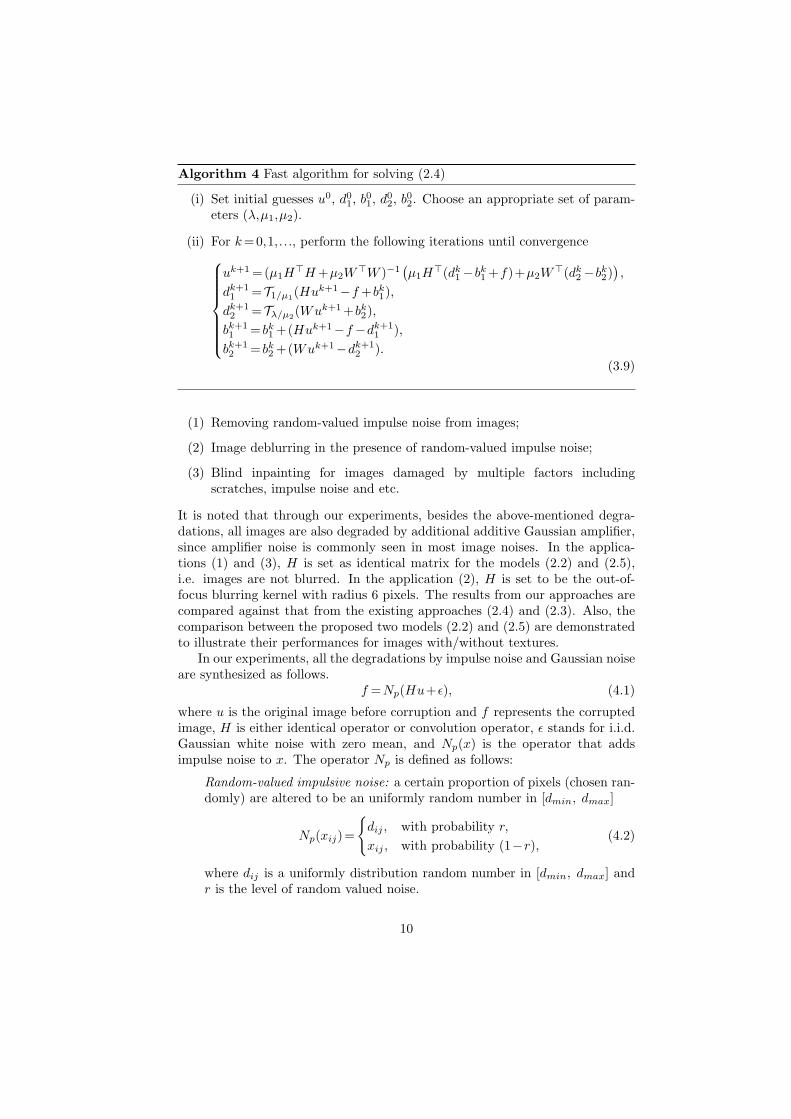
Algorithm 4 Fast algorithm for solving (2.4)

(i) Set initial guesses u0, d01, b01, d

02, b

02. Choose an appropriate set of param-

eters (λ,µ1,µ2).

(ii) For k=0,1,..., perform the following iterations until convergence

uk+1=(µ1H⊤H+µ2W

⊤W )−1(µ1H

⊤(dk1−bk1+f)+µ2W⊤(dk2−bk2)

),

dk+11 =T1/µ1

(Huk+1−f+bk1),

dk+12 =Tλ/µ2

(Wuk+1+bk2),

bk+11 = bk1+(Huk+1−f−dk+1

1 ),

bk+12 = bk2+(Wuk+1−dk+1

2 ).

(3.9)

(1) Removing random-valued impulse noise from images;

(2) Image deblurring in the presence of random-valued impulse noise;

(3) Blind inpainting for images damaged by multiple factors includingscratches, impulse noise and etc.

It is noted that through our experiments, besides the above-mentioned degra-dations, all images are also degraded by additional additive Gaussian amplifier,since amplifier noise is commonly seen in most image noises. In the applica-tions (1) and (3), H is set as identical matrix for the models (2.2) and (2.5),i.e. images are not blurred. In the application (2), H is set to be the out-of-focus blurring kernel with radius 6 pixels. The results from our approaches arecompared against that from the existing approaches (2.4) and (2.3). Also, thecomparison between the proposed two models (2.2) and (2.5) are demonstratedto illustrate their performances for images with/without textures.

In our experiments, all the degradations by impulse noise and Gaussian noiseare synthesized as follows.

f =Np(Hu+ϵ), (4.1)

where u is the original image before corruption and f represents the corruptedimage, H is either identical operator or convolution operator, ϵ stands for i.i.d.Gaussian white noise with zero mean, and Np(x) is the operator that addsimpulse noise to x. The operator Np is defined as follows:

Random-valued impulsive noise: a certain proportion of pixels (chosen ran-domly) are altered to be an uniformly random number in [dmin, dmax]

Np(xij)=

{dij , with probability r,

xij , with probability (1−r),(4.2)

where dij is a uniformly distribution random number in [dmin, dmax] andr is the level of random valued noise.

10

The dynamic range of f which is [dmin, dmax], is taken to be [0,255]. Besidesthe visual comparison of the results, the PSNR measurement is used to quanti-tatively evaluate the quality of the restoration results. Recall that given a signalx, the peak signal to noise ratio (PSNR) of its estimate is defined as

PSNR(x̂,x)=10log102552

1mn

∑mi=1

∑nj=1(x̂ij−xij)2

.

where m and n are the dimensions of the image, xij is the intensity value at thepixel location (i,j), and x̂ij corresponds to the intensity value of the restoredimage at location (i,j).

Through the numerical experiments, 100 iterations are executed in Algo-rithm 1, Algorithm 2 and Algorithm 4 when solving (2.2), (2.5) and (2.4), ittakes approximately 60 seconds when running the matlab implementations ofthese two algorithms on a PC with 2Ghz Intel Core 2 CPU. When solving (2.3),50 iterations of Algorithm 3 are executed which takes about 50 seconds in thesame hardware setting.

4.1. Removing Random-valued Impulse Noise from Images

Besides the most commonly seen Gaussian white noise that degrades images,impulse noise is also often seen in corrupted images due to transmission errors,faulty sensors and etc. There are mainly two types of impulse noise, one issalt-and-pepper noise and the other is random-valued impulse noise. Removingimpulse noise from images is different from removing Gaussian noise as thevalues of damaged pixels contains no information of the truth at all. Thus,removing impulse noise is essentially an image inpainting problem. The pixelsdamaged by salt-and-pepper noise are much easier to find since their brightnessvalues are either 0 or 255. The adaptive median filter has been widely usedto accurately identify most pixels damaged by salt-and-pepper noise (See e.g.[48, 49, 29]). On the contrary, the detection of pixels damaged by random-valued impulse noise is much harder as the brightness value of damaged pixelscan be arbitrary. The adaptive center-weighted median filter (ACWMF) wasfirst proposed in [48] to detect pixels damaged by random-valued impulse noise.More recently, The ROLD detection method has been proposed by [50] withbetter accuracy on detecting such impulse noise. In our experiments, bothdetection techniques are used to provide the input needed for the two-stagemethod (2.3). It is noted that our proposed models do not require the input ofinpainting regions from such a detection pre-process.

The parameters of the proposed denoising algorithms used in the experi-ments are set as follows. For the single system model (2.2), the value of theparameter λ1 is dependent on the level of Gaussian white noise. The higher theGaussian noise level, the larger the value of λ1 should be. Through all experi-ments, the values of λ1 is chosen from the set of {1.8,2,2.25,3}. The value of λ2

is dependent on the impulse noise level and is chosen from {5,6}. The values oftwo parameters λ1,λ2 in (2.5) is set the same as that in (2.2). The value of the

11

parameter λ3 in (2.5) is dependent on the percentage of textures in the givenimage. We set it to 1 for images with less textures and to 5 otherwise.

The PSNR values of the results from all six methods are summarized inTable 1 and Table 2. The visual comparison of some results are shown in Figure 1and Figure 2. From the results, the ROLD detector clearly outperformed theACWMF detector in terms of the accuracy of detecting pixels damaged byimpulse noise. However, when impulse noise is mixed with Gaussian whitenoise, the detection reliability of ROLD detector noticeably decreases as theeffect caused by Gaussian white noise is not considered in the design of theROLD detector. It is seen that the results from our models (2.2) and (2.5) arenoticeably better than (2.4) and (2.3) in terms of PSNR values, especially inthe case of modest noise level. The visual inspection on Figure 1 and Figure 2also leads to the same conclusion. When the impulse noise level is higher,the sparsity assumption of v is less valid. As a result, the performance of ourmodels (2.2) and (2.5) will decrease. However, they still manage to achievemodest gains in image quality, compared to the two-stage method. The resultsin this experiments clearly show the advantages of the models (2.2) and (2.5)by simultaneously identifying outlier and recovering damaged pixels.

It is noted that the proposed two models are not suitable for recovering imagedamaged by very high level of impulse noise, e.g, r=0.6. The main reason isthat the sparsity assumption on the impulse noise does not hold true anymorein such cases. To recover image with very high impulse noise level, the two-stagemethod with impulse noise detector such as ROLD may be a better choice. Onepossible solution is to first detect impulse noise in the image using ROLD in aconservative manner, then use the proposed methods to remove Gaussian noiseand remained un-detected impulse noise from the image..

Table 1: PSNR value (dB) of the denoising results for cameraman image from all the threemodels from (2.3), (2.4) and (2.2) (our model 1), in the presence of random-valued impulsenoise with ratio r and Gaussian noise with std σ.

Ratio r and r = 10% r = 20% r = 40%standard deviation σ=0 σ=10 σ=0 σ=10 σ=0 σ=10

ROLD-ERR Model in [50] 27.4 24.6 25.4 23.6 23.6 22.3

Model (2.3) + ACWMF 28.5 26.0 26.3 24.9 23.1 22.5

Model (2.3) + ROLD 28.4 27.5 26.3 25.8 23.7 23.3

Model (2.4) 29.9 27.5 27.1 26.0 23.1 22.9

Model (2.2) 30.3 28.4 27.4 26.6 23.6 23.3

Model (2.5) 30.3 28.4 27.4 26.6 23.6 23.3

4.2. Image Deblurring in the presence of Random-Valued Impulse Noise

In this application, we applied our blind inpainting algorithm to images thatnot only contain random-valued impulse noise but are also blurry. Same asSection 4.1, we also assume the existence of Gaussian white noise in images.For image deblurring, H in all models are now some convolution matrix and weuse the out-of-focus kernel of radius 6 pixels. The values of parameters λ1,λ2

12

noisy images (2.3) + ROLD (2.4) (2.2)

Figure 1: Denoising results of cameraman image contaminated by both random-valued impulsenoise and Gaussian noise. Images in each column represent (from left to right) corruptedimages, results from (2.3) combined with ROLD pre-detection, results from (2.4) and resultsfrom (2.2) respectively. The noise levels of corrupted images (from top to bottom) are asfollows. (1) 10% random-valued impulse noise without Gaussian noise; (2) 10% random-valued impulse noise with Gaussian noise of σ=10; (3) 20% random-valued impulse noisewithout Gaussian noise (4) 20% random-valued impulse noise with Gaussian noise of σ=10.The PSNR values of the results are given in Table 1.

13

noisy images (2.3) + ROLD (2.4) (2.2)

Figure 2: Denoising result of several images contaminated by random-valued impulse noise ofrate 10% and Gaussian noise of σ=10. Images in each column represent (from left to right)corrupted images, results from (2.3) combined with ROLD pre-detection, results from (2.4)and results from (2.2) respectively. The PSNR values of the results are given in Table 2.

Table 2: PSNR value (dB) of the denoising results for other images from all the three modelsfrom (2.3), (2.4), (2.2) and (2.5), in the presence of random-valued impulse noise with ratio rand Gaussian noise with std=10.

Image and r and Baboon Boat Bridge Barbara512ratio 10% 20% 10% 20% 10% 20% 10% 20%

ROLD-ERR Model in [50] 23.0 21.6 24.7 23.8 23.3 22.1 25.3 23.9

Model (2.3) + ACWMF 23.3 22.2 26.6 25.1 24.2 22.9 26.0 24.6

Model (2.3) + ROLD 24.8 22.9 28.2 26.4 25.3 23.7 27.8 25.8

Model from (2.4) 24.5 23.2 27.6 26.1 25.0 23.4 27.0 25.5

Model from (2.2) 25.1 23.5 28.3 26.4 25.4 23.7 27.9 26.0

Model from (2.5) 25.2 23.5 28.2 26.4 25.4 23.7 27.9 26.0

14

corrupted images (2.3) + ROLD (2.4) (2.2)

Figure 3: Deblurring result of several images in the presence of random-valued impulse noiseof rate 10% and Gaussian noise of σ=10. Images in each column represent (from left to right)corrupted images, results from (2.3) combined with ROLD pre-detection, results from (2.4)and results from (2.2). The PSNR values of the results are given in Table 3.

used in the models are dependent on the noise level and their values are chosenfrom the set {1,10,12}. The PSNR values of the results are summarized inTable 3, and the visual comparison of some results are shown in Figure 3. Itis seen that the results from our models (2.2) and (2.5) are comparable to thatfrom the other two models. Overall, there are not much differences among allfive methods for image deblurring.

Table 3: PSNR value (dB) of the results from (2.3), (2.4), (2.2) and (2.5), for image deblurringin the presence of random-valued impulse noise and Gaussian noise.

Image and r and Cameraman Goldhill Baboonratio 10% 20% 10% 20% 10% 20%

Model (2.3) + ACWMF 24.3 24.0 25.7 21.5 21.2 21.2

Model (2.3) + ROLD 24.3 24.1 25.8 21.6 21.3 21.2

Model (2.4) 24.1 23.9 25.5 21.2 21.2 21.1

Model (2.2) 24.2 24.0 25.7 21.4 21.2 21.1

Model (2.5) 24.2 24.0 25.7 21,4 21.3 21.2

15

corrupted images (2.3) (2.2) (2.5)

Figure 4: The blind inpainting results for images damaged by both impulse noise, scratchand Gaussian noise with std=10. Three sample images are showned (from top to bottom):”Barbara”, ”goldhill” and ”cameraman”. Images in each column represent (from left to right)corrupted image, restored image by (2.3) with ROLD pre-detector, restored image by (2.2)and restored image (2.5). The PSNR values of the results are given in Table 4.

4.3. Blind Inpainting for images damaged by multiple factors

In this application, images are corrupted by both random-valued impulsenoise and scratches without any prior knowledge on their brightness values.The values of parameters λ1,λ2 in both (2.2) and (2.5) are set as λ1=3.5,λ2=5for all images. The value of λ3 in (2.5) is either 1/2 or 1, dependent on thepercentage of textures in the given image.

We compared the results from our proposed models (2.2), (2.5) against thatfrom the two-stage method (2.3) with ROLD pre-detector for detecting bothrandom-valued impulse noise and scratches. The PSNR values of results aresummarized in Table 4 and the results of some sample images are shown inFigure 4. It is seen that the model (2.5) is the best performer among all threemethods, in particular, for ”Barbara512” and ”Goldhill” with rich textures.

The model (2.2) outperformed the model (2.3) with ROLD pre-detector onimages ”Goldhill” and ”Cameraman” which have fewer textures; the model (2.3)with ROLD pre-detector did better on the image ”Barbara512” which has richtextures. The performance of (2.3) is highly dependent on the reliability ofthe ROLD detector on detecting impulse noise. The ROLD detector can notdetect thick scratches and also it cannot reliably detect random-valued impulse

16

noise mixed with Gaussian white noise. As a result, the model (2.3) did notperform well on two images with few textures. The model (2.2) did not do wellon the image with rich textures is because many textures in ”Barbara512” aremis-marked as scratches and been included in v. Thus, the texture region couldbe over-smoothed in (2.2). Such a weakness of (2.2) is addressed in the model(2.5) by including an explicit variable for representing textures. Thus, it is notsurprising to see that the model (2.5) achieved the best performance among allthree methods.

Table 4: PSNR value (dB) of the results for inpainting experiments on images degraded bymixed factors, the rate of random-valued impulse noise is set as 10%.

Standard deviation σImage

of Gaussian noise(2.3) with ROLD (2.2) (2.5)

0 25.2 24.6 25.2Barbara512

10 24.7 24.3 24.70 25.6 26.5 27.2

Goldhill10 24.4 26.0 26.40 23.4 24.8 24.9

Cameraman10 23.3 24.5 24.6

4.4. Conclusions

This paper presents two regularization approaches for blind image inpaintingproblems that are capable of simultaneously identifying corrupted regions andrestoring the corrupted pixels. The basic idea is to utilize the sparsity prior ofimages in wavelet tight frame domain (or/and in discrete local cosine transformdomain) and the sparsity prior of corrupted pixels in the image domain. It isshown in the experiments that the proposed approaches did equally well as orbetter than the existing approaches on some image restoration problems, such asremoving random-valued impulse noise from images or image deblurring in thepresence of random-valued impulse noise. Moreover, the proposed approachesare the first available methods that can automatically recover images corruptedby multiple factors without requiring any user interaction. In future, we willinvestigate the possible applications of the proposed models to other imagerestoration tasks such as blind deconvolution.

References

[1] T. Goldstein, S. Osher, The split Bregman algorithm for L1 regularizedproblems, SIAM Journal on Imaging Sciences 2 (2) (2009) 323–343.

[2] M. Bertalmio, G. Sapiro, V. Caselles, C. Ballester, Image inpainting, in:SIGGRAPH, 2000, pp. 417–424.

17

[3] M. Bertalmio, L. Vese, G. Sapiro, S. Osher, Simultaneous structure andtexture image inpainting, IEEE Transactions on Image Processing 12 (8)(2003) 882–889.

[4] R. Chan, L. Shen, Z. Shen, A framelet-based approach for image inpainting,Research Report 4 (2005) 325.

[5] T. Chan, J. Shen, Variational image inpainting, Commun. Pure Appl. Math58 (2005) 579–619.

[6] T. Chan, J. Shen, H. Zhou, Total variation wavelet inpainting, Journal ofMathematical Imaging and Vision 25 (1) (2006) 107–125.

[7] T. Chan, S. Kang, J. Shen, Euler’s elastica and curvature-based inpainting,SIAM Journal on Applied Mathematics (2002) 564–592.

[8] J. Cai, R. Chan, L. Shen, Z. Shen, Convergence analysis of tight frameletapproach for missing data recovery, Advances in Computational Mathe-matics (2008) 1–27.

[9] J. Cai, R. Chan, Z. Shen, A framelet-based image inpainting algorithm,Applied and Computational Harmonic Analysis 24 (2) (2008) 131–149.

[10] J. Cai, R. Chan, Z. Shen, Simultaneous cartoon and texture inpainting,Inverse Probl. Imaging (to appear).

[11] J. Cai, R. Chan, Z. Shen, A framelet-based image inpainting algorithm,Applied and Computational Harmonic Analysis 24 (2) (2008) 131–149.

[12] Z. Shen, Wavelet frames and image restorations, Proceedings of the Inter-national Congress of Mathematicians, Hyderabad, India.

[13] B. Dong, Z. Shen, MRA based wavelet frames and applications, IAS Lec-ture Notes Series, Summer Program on “The Mathematics of Image Pro-cessing”, Park City Mathematics Institute.

[14] T. F. Chan, J. Shen, Image Processing and Analysis: Variational, PDE,Wavelet, and Stochastic Methods, Society for Industrial Mathematics,2005.

[15] R. C. Gonzalez, R. E. Woods, Digital Image Processing, 2nd Edition, Pren-tice Hall, 2002.

[16] H. Ji, Z. Shen, Y.-H. Xu, Robust video restoration by simultaneous sparseand low-rank matrices decomposition, Tech. rep., NUS (2010).

[17] G. Gilboa, S. Osher, Nonlocal operators with applications to image pro-cessing, Multiscale Model Sim 7 (3) (2008) 1005–1028.

[18] H. Ji, Z. Shen, Y.-H. Xu, Wavelet frame based image restoration withmissing/damaged pixels, East Asia Journal on Applied Mathematics (2011)To appear.

18

[19] A. Ayvaci, M. Raptis, S. Soatto, Optical flow and occlusion detection withconvex optimization, in: Proc. of Neuro Information Processing Systems(NIPS), 2010.

[20] R. Coifman, D. Donoho, Translation-invariant de-noising, Lecture Notes inStatistics-New York-Springer Verlag (1995) 125–125.

[21] E. Candes, D. Donoho, New tight frames of curvelets and optimal represen-tations of objects with C2 singularities, Comm. Pure Appl. Math 56 (2004)219–266.

[22] J. Cai, S. Osher, Z. Shen, Split Bregman methods and frame based imagerestoration, Multiscale Modeling and Simulation: A SIAM InterdisciplinaryJournal 8 (2) (2009) 337–369.

[23] C. Chaux, P. Combettes, J. Pesquet, V. Wajs, A variational formulationfor frame-based inverse problems, Inverse Problems 23 (2007) 1495–1518.

[24] I. Daubechies, G. Teschke, L. Vese, Iteratively solving linear inverse prob-lems under general convex constraints, Inverse Problems and Imaging 1 (1)(2007) 29.

[25] M. Elad, J. Starck, P. Querre, D. Donoho, Simultaneous cartoon and tex-ture image inpainting using morphological component analysis (MCA), Ap-plied and Computational Harmonic Analysis 19 (3) (2005) 340–358.

[26] M. Fadili, J. Starck, F. Murtagh, Inpainting and zooming using sparserepresentations, The Computer Journal 52 (1) (2009) 64.

[27] A. Chai, Z. Shen, Deconvolution: A wavelet frame approach, NumerischeMathematik 106 (4) (2007) 529–587.

[28] T. Goldstein, X. Bresson, S. Osher, Geometric applications of the splitbregman method: Segmentation and surface reconstruction, Journal of Sci-entific Computing 45 (1) (2009) 272–293.

[29] J. Cai, S. Osher, Z. Shen, Linearized Bregman iterations for compressedsensing, Math. Comp 78 (2009) 1515–1536.

[30] I. Daubechies, Ten lectures on wavelets, Society for Industrial Mathematics,1992.

[31] A. Ron, Z. Shen, Affine Systems in L2(Rd): The Analysis of the AnalysisOperator, Journal of Functional Analysis 148 (2) (1997) 408–447.

[32] I. Daubechies, B. Han, A. Ron, Z. Shen, Framelets: MRA-based construc-tions of wavelet frames, Applied and Computational Harmonic Analysis14 (1) (2003) 1–46.

[33] J. Cai, M. Nikolova, R. Chan, Fast two-phase image deblurring under im-pulse noise, J. Math. Imaging Vis. 36 (2010) 46–53.

19

[34] L. Bar, N. Kiryati, N. Sochen, Image deblurring in the presence of impulsenoise, International Journal of Computer Vision 70 (3) (2006) 279–298.

[35] L. Bar, N. Sochen, N. Kiryati, Image deblurring in the presence of salt-and-pepper noise, in: Lecture Notes in Computer Science, Scale Space andPDE Methods in Computer Vision, LNCS), Vol. 3459, 2005, pp. 107–118.

[36] G. Healey, R. Kondepudy, Radiometric ccd camera calibration and noiseestimation, IEEE Trans. PAMI 16 (3) (1994) 267–276.

[37] S. Alliney, Digital filters as absolute norm regularizers, IEEE Transactionson Signal Processing 40 (6) (1992) 1548–1562.

[38] T. Chan, S. Esedoglu, Aspects of Total Variation Regularized L1 FunctionApproximation, SIAM Journal on Applied Mathematics 65 (5) (2005) 1817.

[39] M. Nikolova, A variational approach to remove outliers and impulse noise,Journal of Mathematical Imaging and Vision 20 (1) (2004) 99–120.

[40] X. Zhang, M. Burger, X. Bresson, S. Osher, Bregmanized nonlocal regu-larization for deconvolution and sparse reconstruction, SIAM Journal onImaging Sciences 3 (1) (2010) 253–276.

[41] E. Esser, Applications of Lagrangian-based alternating direction methodsand connections to split Bregman, Tech. Rep. TR 09-31, UCLA (March2009).

[42] X. Tai, C. Wu, Augmented Lagrangian method, dual methods and splitBregman iteration for ROF model, Scale Space and Variational Methodsin Computer Vision (2009) 502–513.

[43] R. Glowinski, P. Le Tallec, Augmented Lagrangian and operator-splittingmethods in nonlinear mechanics, Society for Industrial Mathematics, 1989.

[44] S. Setzer, Split Bregman algorithm, Douglas-Rachford splitting and frameshrinkage, Scale Space and Variational Methods in Computer Vision (2009)464–476.

[45] D. Donoho, De-noising by soft-thresholding, IEEE transactions on infor-mation theory 41 (3) (1995) 613–627.

[46] P. Combettes, V. Wajs, Signal recovery by proximal forward-backwardsplitting, Multiscale Modeling and Simulation 4 (4) (2006) 1168–1200.

[47] B. Dong, E. Savitsky, S. Osher, A Novel Method for Enhanced NeedleLocalization Using Ultrasound-Guidance, Advances in Visual Computing(2009) 914–923.

[48] T. Chen, H. R. Wu, Adaptive impulse dectection using center-weightedmedian filters, IEEE Signal Processing Letters 8 (1) (2001) 1–3.

20

[49] H. Hwang, R. Haddad, Adaptive median filters: new algorithms and results,IEEE Transactions on Image Processing 4 (4) (1995) 499–502.

[50] Y. Dong, R. F. Chan, S. Xu, A detection statistic for random-valued im-pulse noise, IEEE Transactions on Image Processing 16 (4) (2007) 1112–1120.

21