Embed Size (px)
DESCRIPTION
DSRC/WAVE Tutorial
Citation preview
The WAVE Solution – Coming Soon to a Car Near You: Wireless Access
Dr. Guillermo AcostaProfessor Roberto A. Uzcategui
Introduction
2Guillermo Acosta and Roberto Uzcategui
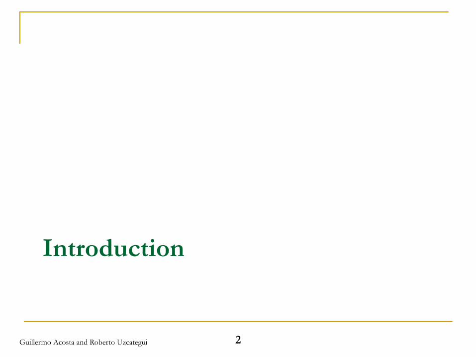
The OSI Reference ModelOSI: Open Systems Interconnection.Abstract description of a layered computer network.Divides network architecture into seven layers: Application, Presentation, Session, Transport, Network, Data Link, and Physical.⇒ Also known as The Seven Layer Model.More historic and didactic than currently archetypal.
Excellent place to start studying network architecture, even though actual systems might not easily fit the model.Most widespread network architecture (TCP/IP) does not fit Seven Layer Model (it has five layers).
3Guillermo Acosta and Roberto Uzcategui
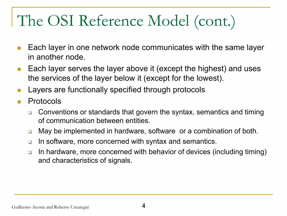
The OSI Reference Model (cont.)Each layer in one network node communicates with the same layer in another node.Each layer serves the layer above it (except the highest) and uses the services of the layer below it (except for the lowest).Layers are functionally specified through protocolsProtocols
Conventions or standards that govern the syntax, semantics and timing of communication between entities.May be implemented in hardware, software or a combination of both.In software, more concerned with syntax and semantics.In hardware, more concerned with behavior of devices (including timing) and characteristics of signals.
4Guillermo Acosta and Roberto Uzcategui
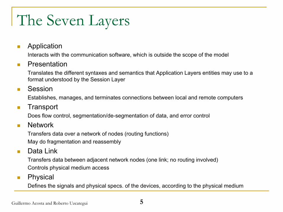
The Seven LayersApplicationInteracts with the communication software, which is outside the scope of the model
PresentationTranslates the different syntaxes and semantics that Application Layers entities may use to a format understood by the Session Layer
SessionEstablishes, manages, and terminates connections between local and remote computers
TransportDoes flow control, segmentation/de-segmentation of data, and error control
NetworkTransfers data over a network of nodes (routing functions)May do fragmentation and reassembly
Data LinkTransfers data between adjacent network nodes (one link; no routing involved)Controls physical medium access
PhysicalDefines the signals and physical specs. of the devices, according to the physical medium
5Guillermo Acosta and Roberto Uzcategui
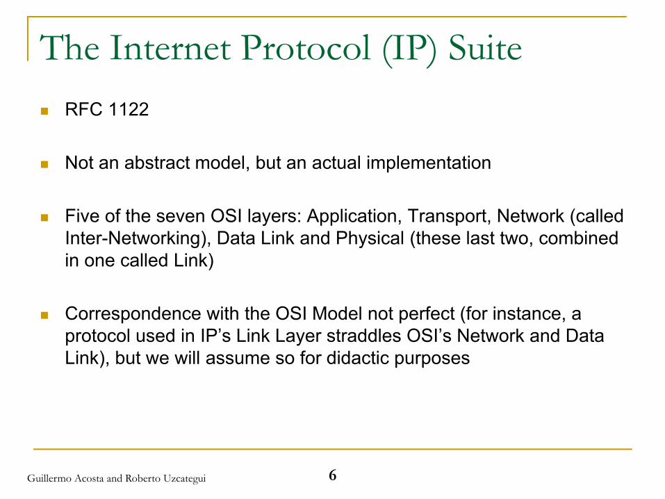
The Internet Protocol (IP) SuiteRFC 1122
Not an abstract model, but an actual implementation
Five of the seven OSI layers: Application, Transport, Network (called Inter-Networking), Data Link and Physical (these last two, combined in one called Link)
Correspondence with the OSI Model not perfect (for instance, a protocol used in IP’s Link Layer straddles OSI’s Network and Data Link), but we will assume so for didactic purposes
6Guillermo Acosta and Roberto Uzcategui
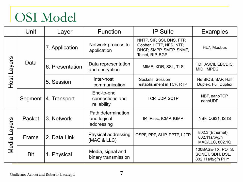
OSI ModelUnit Layer Function IP Suite Examples
Hos
t Lay
ers
Data
7. Application Network process to application
NNTP, SIP, SSI, DNS, FTP, Gopher, HTTP, NFS, NTP, DHCP, SMPP, SMTP, SNMP, Telnet, RIP, BGP
HL7, Modbus
6. Presentation Data representation and encryption MIME, XDR, SSL, TLS TDI, ASCII, EBCDIC,
MIDI, MPEG
5. Session Inter-host communication
Sockets. Session establishment in TCP, RTP
NetBIOS, SAP, Half Duplex, Full Duplex
Segment 4. TransportEnd-to-end connections and reliability
TCP, UDP, SCTP NBF, nanoTCP, nanoUDP
Med
ia L
ayer
s Packet 3. NetworkPath determination and logicaladdressing
IP, IPsec, ICMP, IGMP NBF, Q.931, IS-IS
Frame 2. Data Link Physical addressing (MAC & LLC)
OSPF, PPP, SLIP, PPTP, L2TP 802.3 (Ethernet), 802.11a/b/g/n MAC/LLC, 802.1Q
Bit 1. Physical Media, signal and binary transmission
100BASE-TX, POTS, SONET, SDH, DSL, 802.11a/b/g/n PHY
7Guillermo Acosta and Roberto Uzcategui
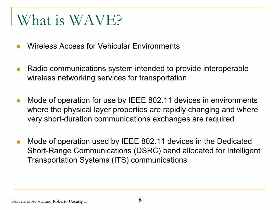
What is WAVE?Wireless Access for Vehicular Environments
Radio communications system intended to provide interoperable wireless networking services for transportation
Mode of operation for use by IEEE 802.11 devices in environments where the physical layer properties are rapidly changing and where very short-duration communications exchanges are required
Mode of operation used by IEEE 802.11 devices in the Dedicated Short-Range Communications (DSRC) band allocated for Intelligent Transportation Systems (ITS) communications
8Guillermo Acosta and Roberto Uzcategui
Why WAVE?
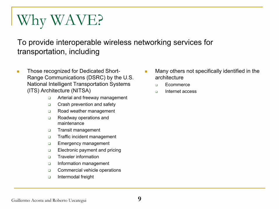
Those recognized for Dedicated Short-Range Communications (DSRC) by the U.S. National Intelligent Transportation Systems (ITS) Architecture (NITSA)
Arterial and freeway managementCrash prevention and safetyRoad weather managementRoadway operations and maintenanceTransit managementTraffic incident managementEmergency managementElectronic payment and pricingTraveler informationInformation managementCommercial vehicle operationsIntermodal freight
Many others not specifically identified in the architecture
EcommerceInternet access
To provide interoperable wireless networking services for transportation, including
9Guillermo Acosta and Roberto Uzcategui
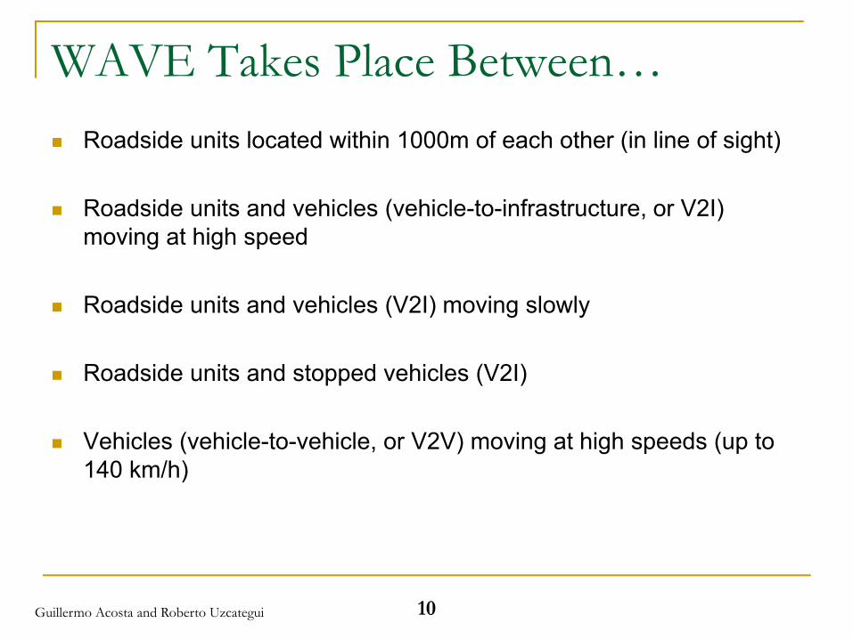
WAVE Takes Place Between…Roadside units located within 1000m of each other (in line of sight)
Roadside units and vehicles (vehicle-to-infrastructure, or V2I) moving at high speed
Roadside units and vehicles (V2I) moving slowly
Roadside units and stopped vehicles (V2I)
Vehicles (vehicle-to-vehicle, or V2V) moving at high speeds (up to 140 km/h)
10Guillermo Acosta and Roberto Uzcategui
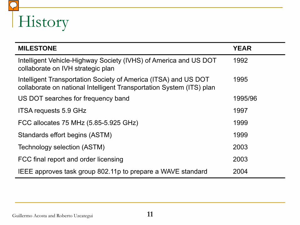
HistoryMILESTONE YEAR
Intelligent Vehicle-Highway Society (IVHS) of America and US DOT collaborate on IVH strategic plan
1992
Intelligent Transportation Society of America (ITSA) and US DOT collaborate on national Intelligent Transportation System (ITS) plan
1995
US DOT searches for frequency band 1995/96
ITSA requests 5.9 GHz 1997
FCC allocates 75 MHz (5.85-5.925 GHz) 1999
Standards effort begins (ASTM) 1999
Technology selection (ASTM) 2003
FCC final report and order licensing 2003
IEEE approves task group 802.11p to prepare a WAVE standard 2004
11Guillermo Acosta and Roberto Uzcategui
Why Base WAVE on 802.11?To have a stable standard supported by experts in wireless technology.
Necessary to guarantee interoperability between vehicles made by different manufacturers.Necessary to guarantee interoperability with roadside infrastructure in different geographic locations.
To guarantee that the standard will be maintained in concert with other ongoing developments in IEEE 802.11.
Since 802.11p is based o 802.11a, synergies in chipset design are expected to help ensure the necessary production economies of scale.
12Guillermo Acosta and Roberto Uzcategui
Why a Different Version of 802.11?Changes are required to support
The longer ranges of operation (up to 1000 m)The high speed of the vehiclesThe extreme multipath environmentThe need for multiple overlapping ad-hoc networks to operate with extremely high quality of serviceThe nature of the applications to be executedA special type of beacon frame, used only in the ITS (DSRC) frequency band
13Guillermo Acosta and Roberto Uzcategui
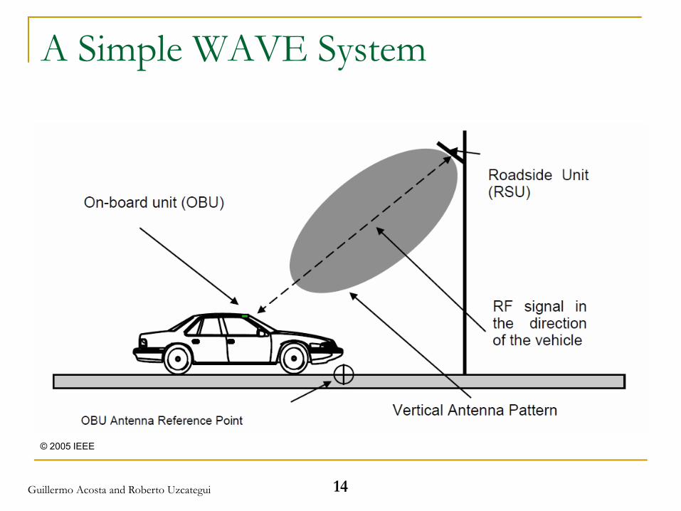
A Simple WAVE System
© 2005 IEEE
14Guillermo Acosta and Roberto Uzcategui
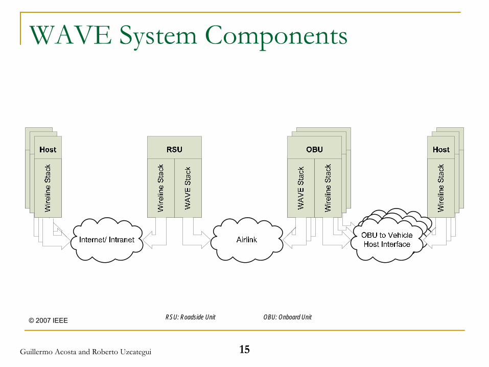
WAVE System Components
© 2007 IEEE RSU: Roadside Unit OBU: Onboard Unit
15Guillermo Acosta and Roberto Uzcategui
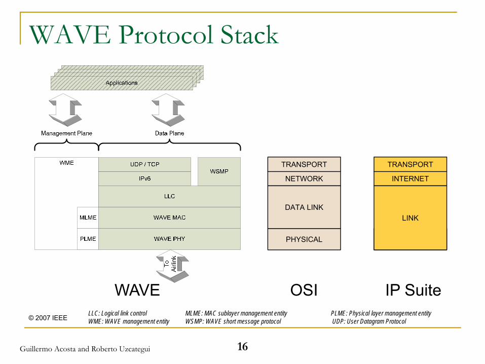
WAVE Protocol Stack
WAVE
PHYSICAL
NETWORK
TRANSPORT
DATA LINK
OSI
PHYSICAL
INTERNET
TRANSPORT
LINK
IP SuiteLLC: Logical link control MLME: MAC sublayer management entity PLME: Physical layer management entityWME: WAVE management entity WSMP: WAVE short message protocol UDP: User Datagram Protocol© 2007 IEEE
16Guillermo Acosta and Roberto Uzcategui
Background
17Guillermo Acosta and Roberto Uzcategui
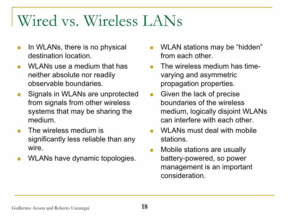
Wired vs. Wireless LANsIn WLANs, there is no physical destination location.WLANs use a medium that has neither absolute nor readily observable boundaries.Signals in WLANs are unprotected from signals from other wireless systems that may be sharing the medium.The wireless medium is significantly less reliable than any wire.WLANs have dynamic topologies.
WLAN stations may be “hidden” from each other.The wireless medium has time-varying and asymmetric propagation properties.Given the lack of precise boundaries of the wireless medium, logically disjoint WLANs can interfere with each other.WLANs must deal with mobile stations.Mobile stations are usually battery-powered, so power management is an important consideration.
18Guillermo Acosta and Roberto Uzcategui
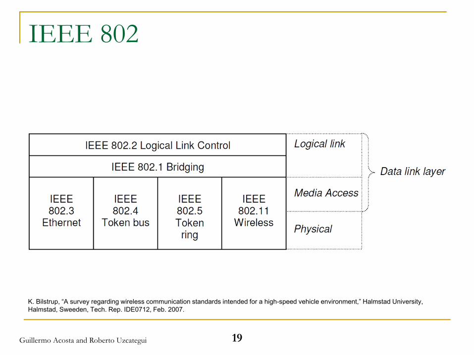
IEEE 802
K. Bilstrup, “A survey regarding wireless communication standards intended for a high-speed vehicle environment,” Halmstad University,Halmstad, Sweeden, Tech. Rep. IDE0712, Feb. 2007.
19Guillermo Acosta and Roberto Uzcategui
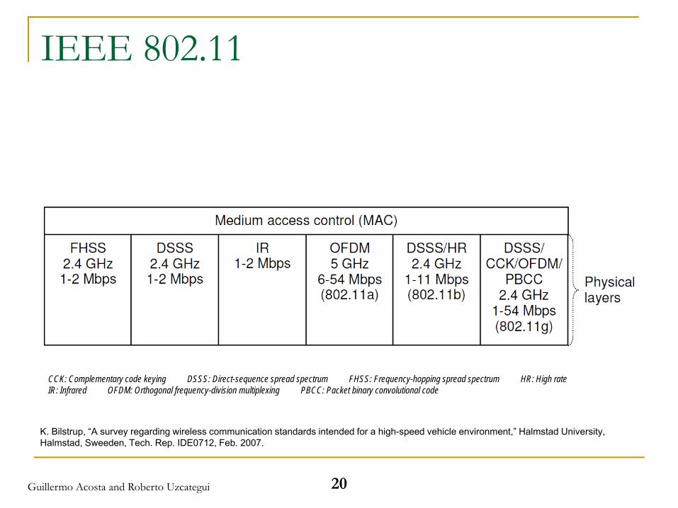
IEEE 802.11
K. Bilstrup, “A survey regarding wireless communication standards intended for a high-speed vehicle environment,” Halmstad University,Halmstad, Sweeden, Tech. Rep. IDE0712, Feb. 2007.
CCK: Complementary code keying DSSS: Direct-sequence spread spectrum FHSS: Frequency-hopping spread spectrum HR: High rateIR: Infrared OFDM: Orthogonal frequency-division multiplexing PBCC: Packet binary convolutional code
20Guillermo Acosta and Roberto Uzcategui
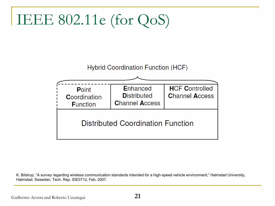
IEEE 802.11e (for QoS)
K. Bilstrup, “A survey regarding wireless communication standards intended for a high-speed vehicle environment,” Halmstad University,Halmstad, Sweeden, Tech. Rep. IDE0712, Feb. 2007.
21Guillermo Acosta and Roberto Uzcategui
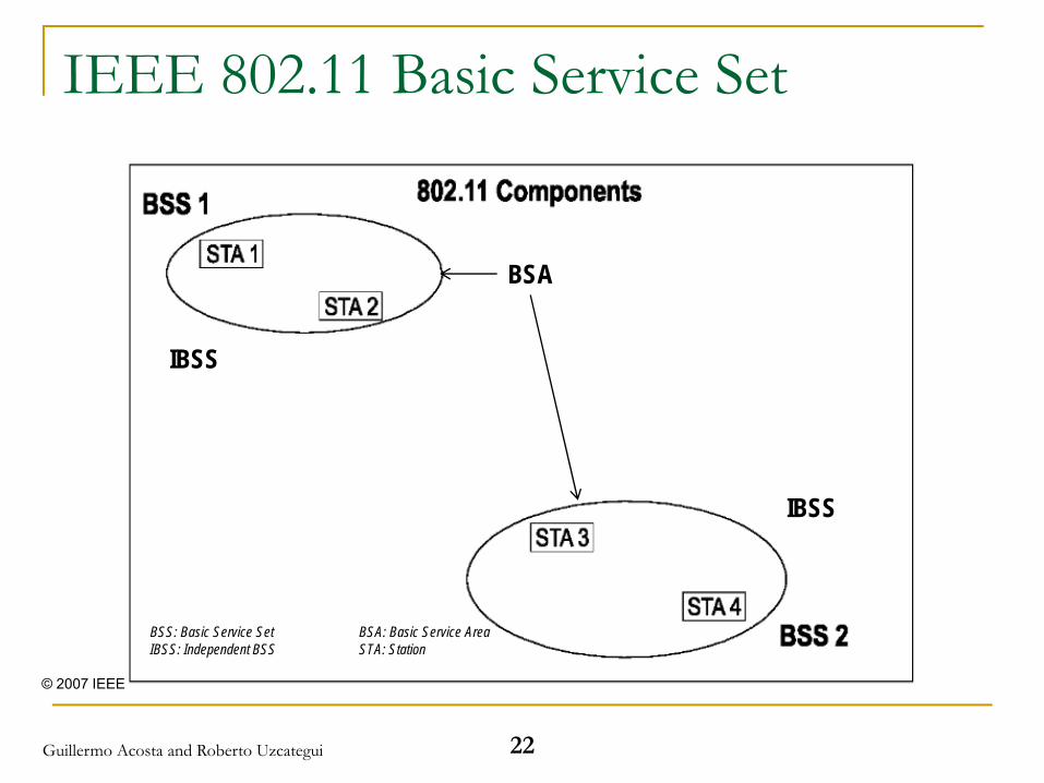
IEEE 802.11 Basic Service Set
BSA
IBSS
IBSS
BSS: Basic Service Set BSA: Basic Service AreaIBSS: Independent BSS STA: Station
© 2007 IEEE
22Guillermo Acosta and Roberto Uzcategui
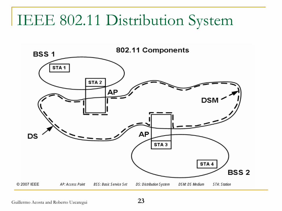
IEEE 802.11 Distribution System
AP: Access Point BSS: Basic Service Set DS: Distribution System DSM: DS Medium STA: Station© 2007 IEEE
23Guillermo Acosta and Roberto Uzcategui
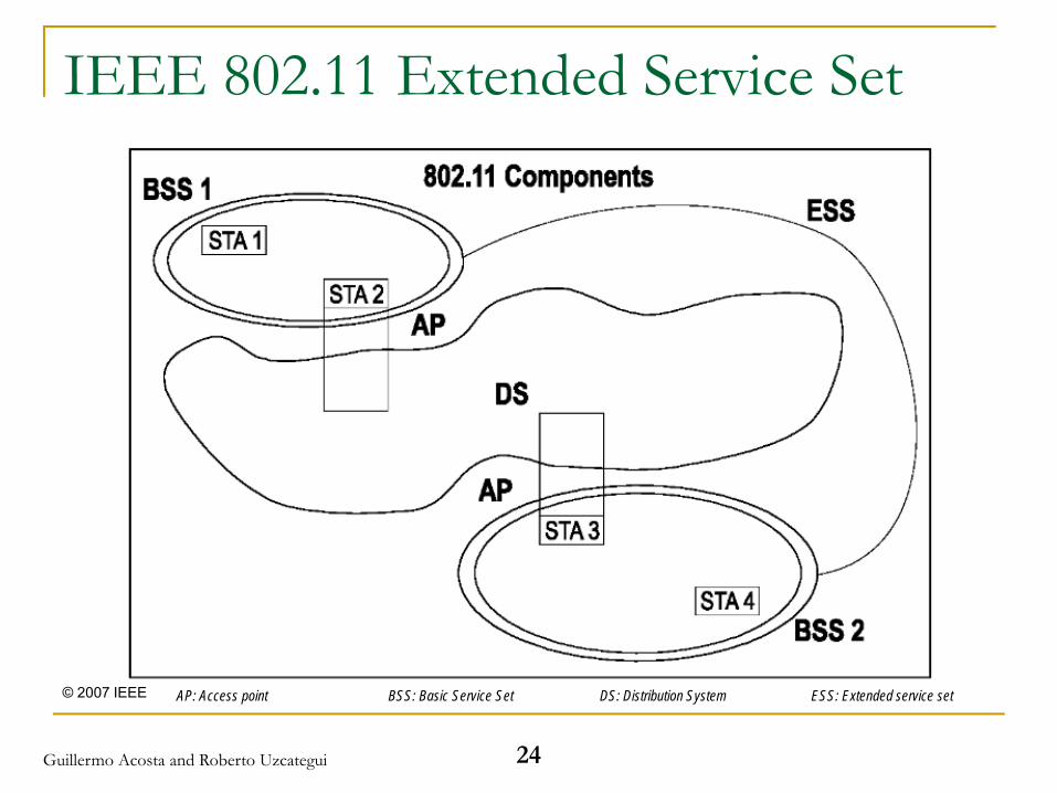
IEEE 802.11 Extended Service Set
AP: Access point BSS: Basic Service Set DS: Distribution System ESS: Extended service set© 2007 IEEE
24Guillermo Acosta and Roberto Uzcategui
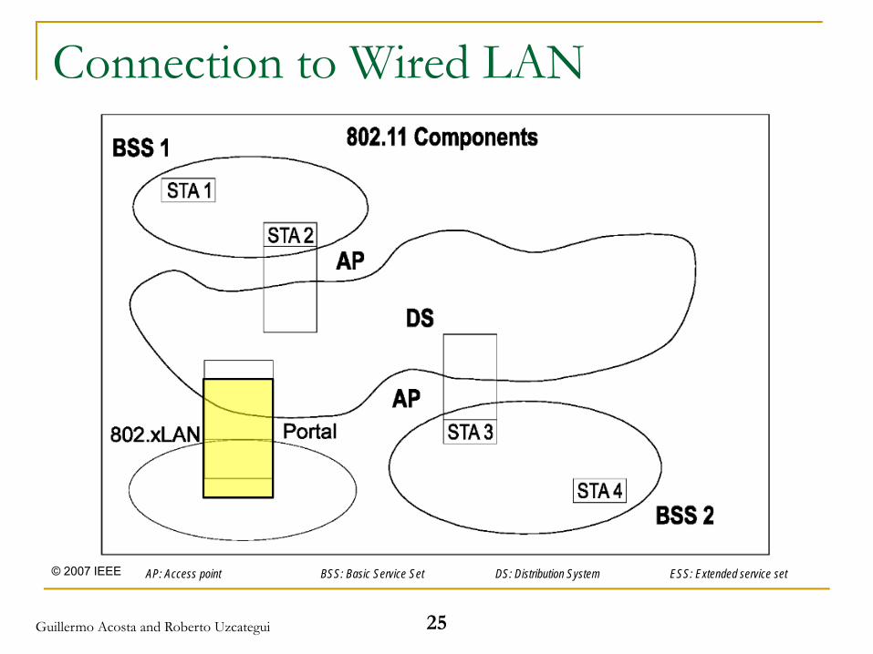
Connection to Wired LAN
© 2007 IEEE AP: Access point BSS: Basic Service Set DS: Distribution System ESS: Extended service set
25Guillermo Acosta and Roberto Uzcategui
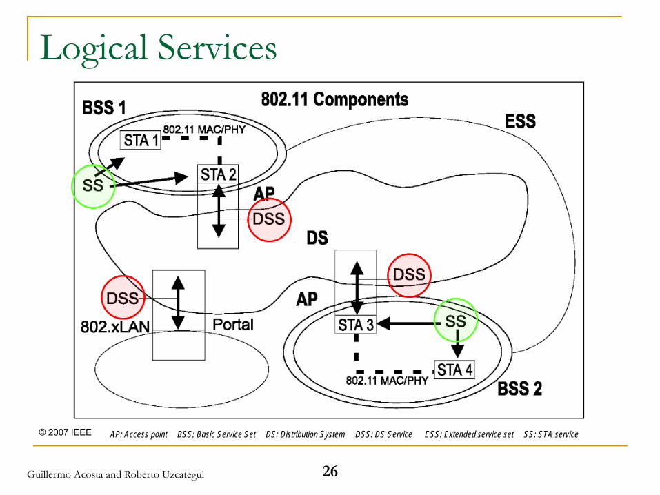
Logical Services
© 2007 IEEE AP: Access point BSS: Basic Service Set DS: Distribution System DSS: DS Service ESS: Extended service set SS: STA service
26Guillermo Acosta and Roberto Uzcategui
Logical Services (cont.)
SS: services provided by STAs
AuthenticationDe-authenticationData confidentialityMAC Service Data Unit (MSDU) deliveryDynamic Frequency Selection (DFS)Transmit Power Control (TPC)Higher-layer timer synchronizationQoS traffic scheduling
DSS: services provided by the DS
AssociationDisassociationDistributionIntegrationRe-associationQoS traffic scheduling
27Guillermo Acosta and Roberto Uzcategui
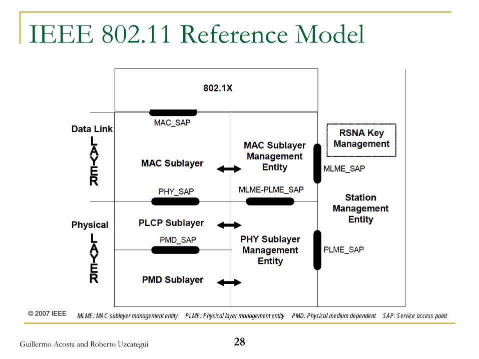
IEEE 802.11 Reference Model
© 2007 IEEE MLME: MAC sublayer management entity PLME: Physical layer management entity PMD: Physical medium dependent SAP: Service access point
28Guillermo Acosta and Roberto Uzcategui
WAVE
29Guillermo Acosta and Roberto Uzcategui
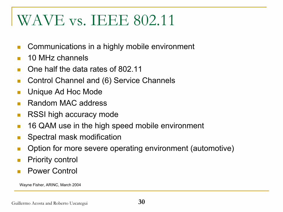
WAVE vs. IEEE 802.11Communications in a highly mobile environment10 MHz channelsOne half the data rates of 802.11Control Channel and (6) Service ChannelsUnique Ad Hoc Mode Random MAC addressRSSI high accuracy mode16 QAM use in the high speed mobile environmentSpectral mask modificationOption for more severe operating environment (automotive)Priority control Power Control
Wayne Fisher, ARINC, March 2004
30Guillermo Acosta and Roberto Uzcategui
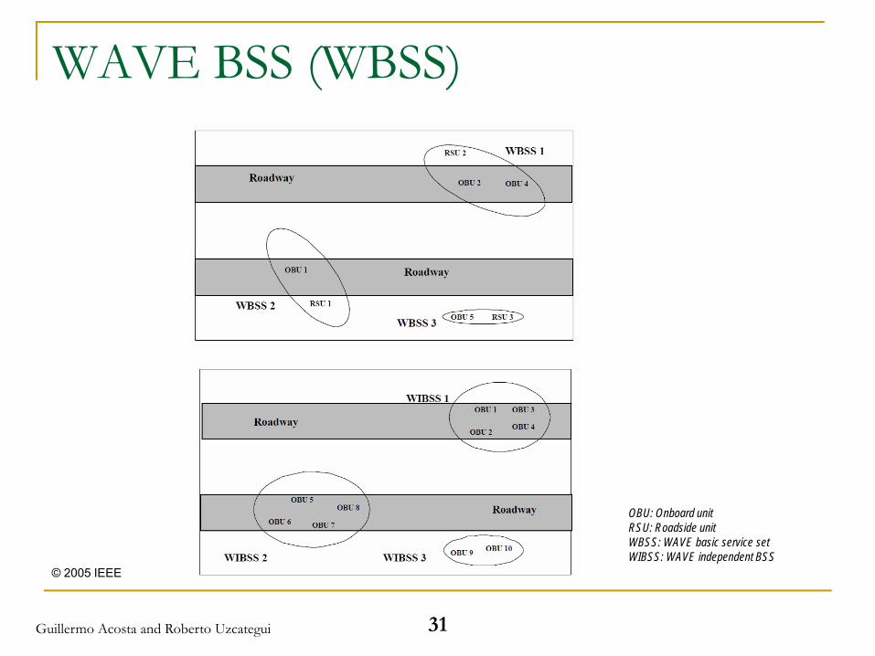
WAVE BSS (WBSS)
© 2005 IEEE
OBU: Onboard unitRSU: Roadside unitWBSS: WAVE basic service setWIBSS: WAVE independent BSS
31Guillermo Acosta and Roberto Uzcategui
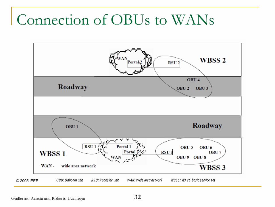
Connection of OBUs to WANs
© 2005 IEEE OBU: Onboard unit RSU: Roadside unit WAN: Wide area network WBSS: WAVE basic service set
32Guillermo Acosta and Roberto Uzcategui
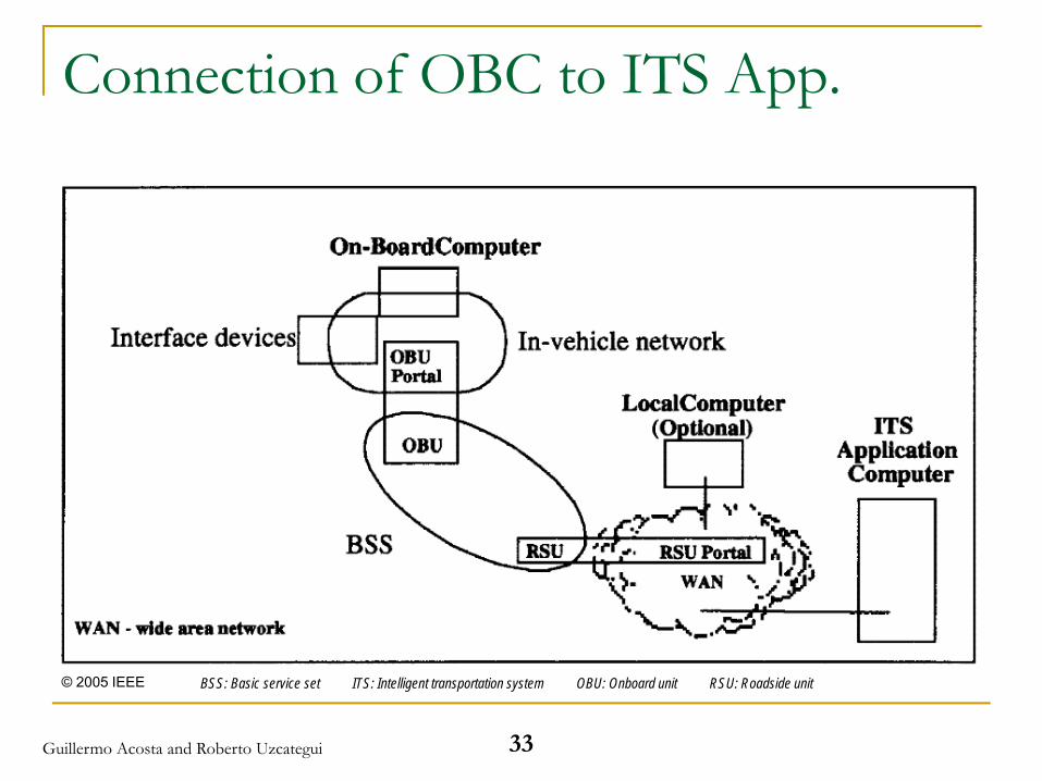
Connection of OBC to ITS App.
© 2005 IEEE BSS: Basic service set ITS: Intelligent transportation system OBU: Onboard unit RSU: Roadside unit
33Guillermo Acosta and Roberto Uzcategui

Connection of OBU to OBC
© 2005 IEEE
34Guillermo Acosta and Roberto Uzcategui
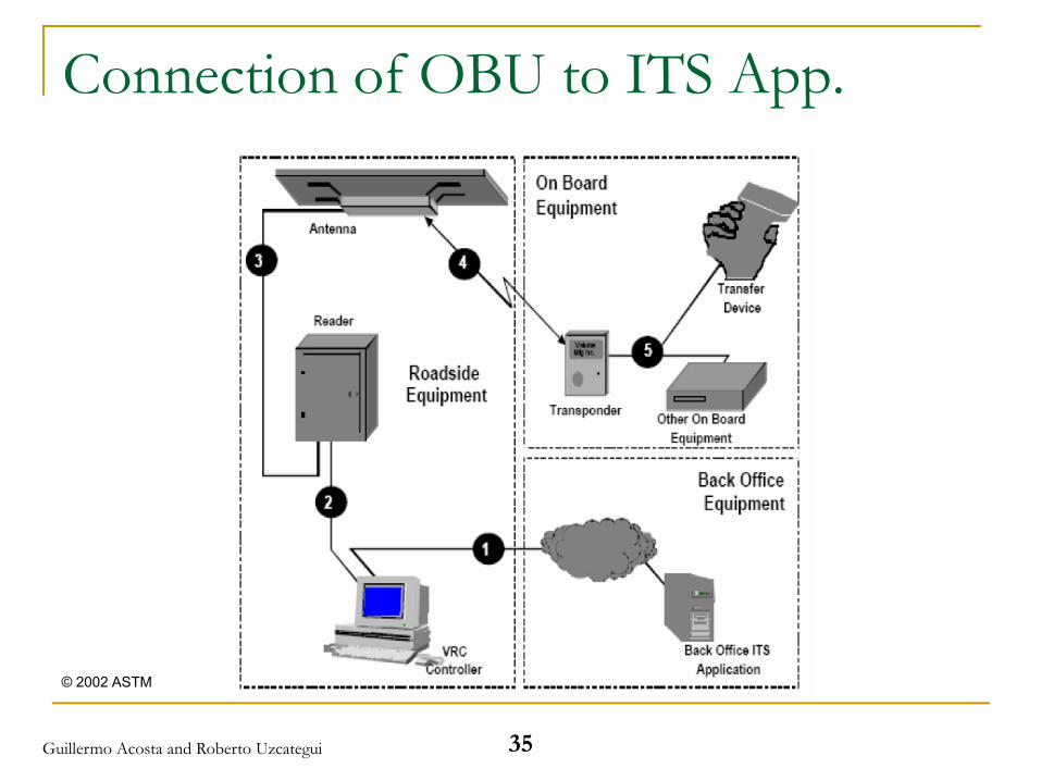
Connection of OBU to ITS App.
© 2002 ASTM
35Guillermo Acosta and Roberto Uzcategui
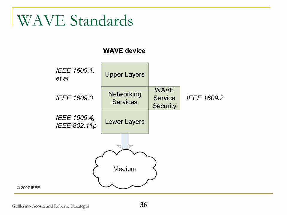
WAVE Standards
© 2007 IEEE
36Guillermo Acosta and Roberto Uzcategui
Purpose of IEEE 1609.1OBUs may want to use services provided by applications installed in units far removed from the RSUs.
OBUs host an application (Resource Command Processor, or RCP) that uses the service. Third parties (remote from the RSUs) host other applications (Resource Manager Applications, or RMAs) that provide the services.RSUs host an application (Resource Manager, or RM) that acts as middle-man between RCPs and RMAs.
This standard specifies the RM and the RCP. This standard describes how the RM multiplexes requests from multiple RMA, each of which is communicating with multiple OBUs hosting a RCP. The purpose of the communication is to provide the RMA access to “resources” such as memory, user interfaces and interfaces to other on-board equipment controlled by the RCP, in a consistent, interoperable and timely manner to meet the requirements of RMA.
37Guillermo Acosta and Roberto Uzcategui
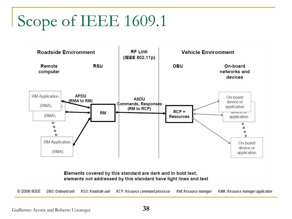
Scope of IEEE 1609.1
© 2006 IEEE OBU: Onboard unit RSU: Roadside unit RCP: Resource command processor RM: Resource manager RMA: Resource manager application
38Guillermo Acosta and Roberto Uzcategui
Purpose of IEEE 1609.2To define secure formats for management and application messages, and the processing of those secure messagesTo protect from attacks such as
EavesdroppingSpoofingAlterationReplayInvasion of privacy
To guaranteeConfidentialityIntegrityAuthenticityAnonymity
39Guillermo Acosta and Roberto Uzcategui
Purpose of IEEE 1609.3
WAVE networking services
Layers 3 and 4 of the OSI communications stack
Addressing and routing services within a WAVE system
40Guillermo Acosta and Roberto Uzcategui
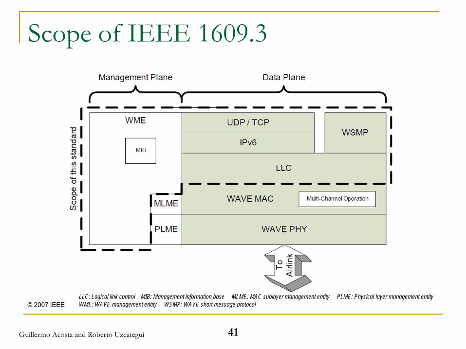
Scope of IEEE 1609.3
© 2007 IEEELLC: Logical link control MIB: Management information base MLME: MAC sublayer management entity PLME: Physical layer management entityWME: WAVE management entity WSMP: WAVE short message protocol
41Guillermo Acosta and Roberto Uzcategui
Purpose of IEEE 1609.4Multichannel wireless radio operation over WAVE PHY and MAC layers
Operation of control and service channels
Operation of interval timers
Priority access
Channel switching and routing
Management services
42Guillermo Acosta and Roberto Uzcategui
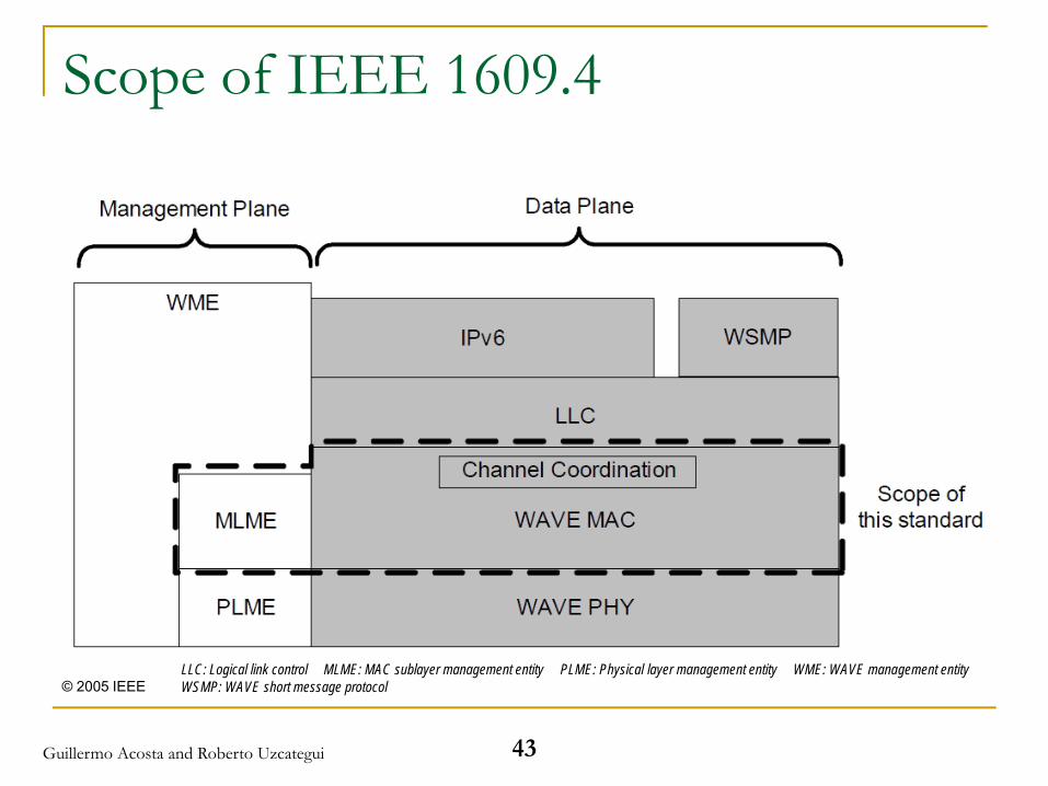
Scope of IEEE 1609.4
© 2005 IEEELLC: Logical link control MLME: MAC sublayer management entity PLME: Physical layer management entity WME: WAVE management entityWSMP: WAVE short message protocol
43Guillermo Acosta and Roberto Uzcategui
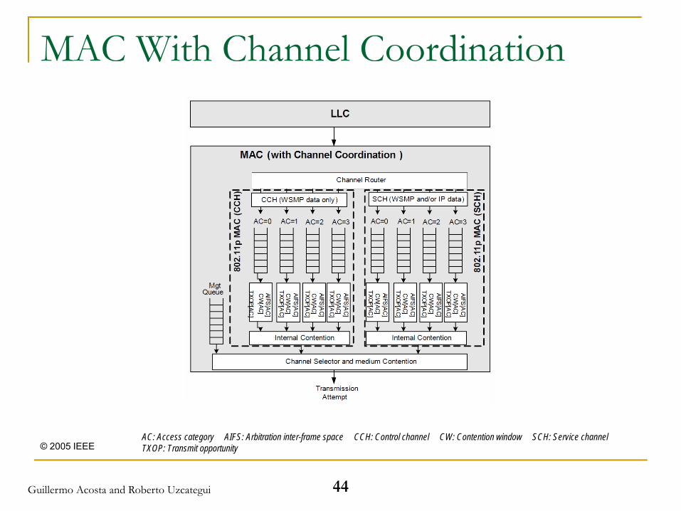
MAC With Channel Coordination
© 2005 IEEEAC: Access category AIFS: Arbitration inter-frame space CCH: Control channel CW: Contention window SCH: Service channelTXOP: Transmit opportunity
44Guillermo Acosta and Roberto Uzcategui
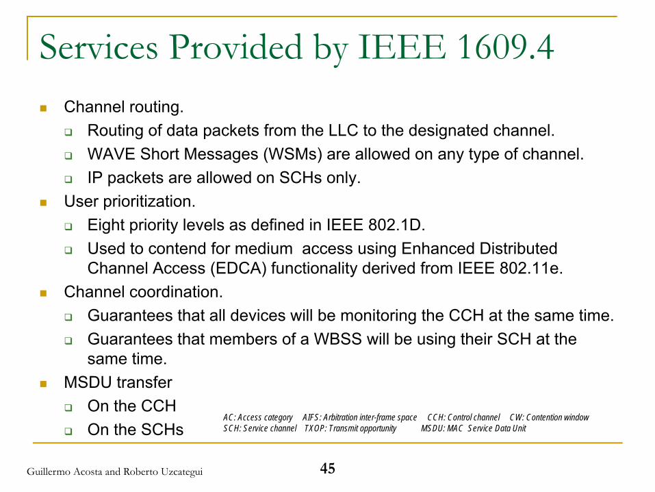
Services Provided by IEEE 1609.4Channel routing.
Routing of data packets from the LLC to the designated channel.WAVE Short Messages (WSMs) are allowed on any type of channel.IP packets are allowed on SCHs only.
User prioritization.Eight priority levels as defined in IEEE 802.1D.Used to contend for medium access using Enhanced Distributed Channel Access (EDCA) functionality derived from IEEE 802.11e.
Channel coordination.Guarantees that all devices will be monitoring the CCH at the same time.Guarantees that members of a WBSS will be using their SCH at the same time.
MSDU transferOn the CCHOn the SCHs
AC: Access category AIFS: Arbitration inter-frame space CCH: Control channel CW: Contention window SCH: Service channel TXOP: Transmit opportunity MSDU: MAC Service Data Unit
45Guillermo Acosta and Roberto Uzcategui
IEEE 802.11p
46Guillermo Acosta and Roberto Uzcategui
Medium Access Control Layer
47Guillermo Acosta and Roberto Uzcategui
Purpose of the MAC LayerChannel-access control
Mechanisms usually known as multiple access protocolsMay detect or avoid data-packet collisions (contention based protocols)May establish logical channels (channelization based protocols)Examples:
In Ethernet, Carrier Sense Multiple Access/Collision Detection (CSMA/CD)In WLANs, Carrier Sense Multiple Access/Collision Avoidance (CSMA/CA)
AddressingUnique serial number assigned to each network adapter, known as MAC AddressMakes it possible to deliver data packets to a destination within a subnetwork , i.e. a physical network consisting of one or several network segments interconnected by repeaters, hubs, bridges and switches, but not by IP routers
48Guillermo Acosta and Roberto Uzcategui
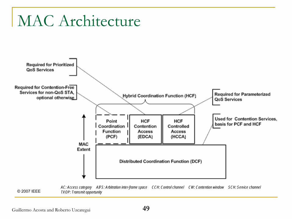
MAC Architecture
© 2007 IEEEAC: Access category AIFS: Arbitration inter-frame space CCH: Control channel CW: Contention window SCH: Service channelTXOP: Transmit opportunity
49Guillermo Acosta and Roberto Uzcategui
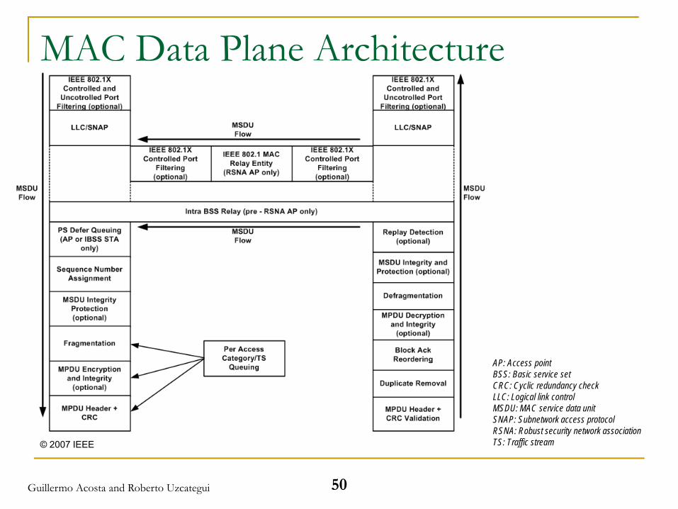
MAC Data Plane Architecture
© 2007 IEEE
AP: Access pointBSS: Basic service setCRC: Cyclic redundancy checkLLC: Logical link controlMSDU: MAC service data unitSNAP: Subnetwork access protocolRSNA: Robust security network associationTS: Traffic stream
50Guillermo Acosta and Roberto Uzcategui
Channel TypesA single Control Channel (CCH)
Reserved for short, high-priority application and system control messagesBy default, WAVE devices operate here
Multiple Service Channels (SCHs)For general-purpose application data transfersVisits are arranged via a WBSS (WAVE Basic Service Set)
51Guillermo Acosta and Roberto Uzcategui

Channel CoordinationSynchronized scheme based on Coordinated Universal Time (UTC).Assures that all WAVE devices will be monitoring the CCH during a common time interval (CCH Interval).Assures that members of a WBSS will be using the corresponding SCH during a common time interval (SCH Interval).The sum of the CCH and SCH intervals comprises a Sync Interval.At the start of a Sync Interval, all devices must monitor the CCH.There are 10 Sync intervals per UTC second.Channel intervals are padded with a guard interval.
© 2005 IEEE
AC: Access category AIFS: Arbitration inter-frame space CCH: Control channel CW: Contention window SCH: Service channel TXOP: Transmit opportunity
52Guillermo Acosta and Roberto Uzcategui
Communication ProtocolsWAVE accommodates two protocol stacks:
Standard Internet Protocol (IPv6).WAVE Short Message Protocol (WSMP).
WAVE Short Messages (WSMs) may be sent on any channel.
IP messages may be sent only on SCHs.
System management frames are sent on the CCH.
WSMP allows applications to directly control PHY characteristics, such as channel number and transmitter power.
53Guillermo Acosta and Roberto Uzcategui
AC: Access category AIFS: Arbitration inter-frame space CCH: Control channel CW: Contention window SCH: Service channelTXOP: Transmit opportunity
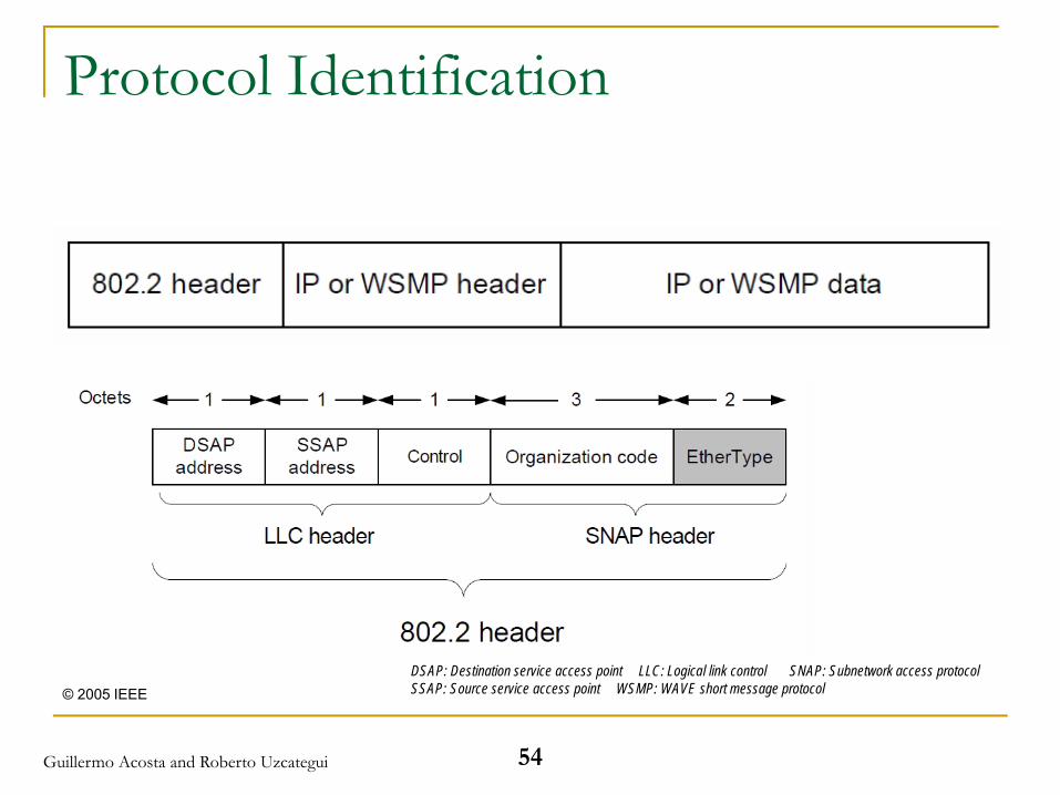
Protocol Identification
DSAP: Destination service access point LLC: Logical link control SNAP: Subnetwork access protocolSSAP: Source service access point WSMP: WAVE short message protocol© 2005 IEEE
54Guillermo Acosta and Roberto Uzcategui
Physical Layer
55Guillermo Acosta and Roberto Uzcategui
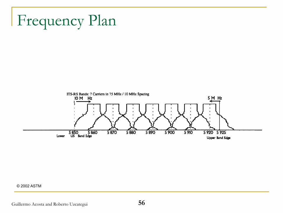
Frequency Plan
© 2002 ASTM
56Guillermo Acosta and Roberto Uzcategui
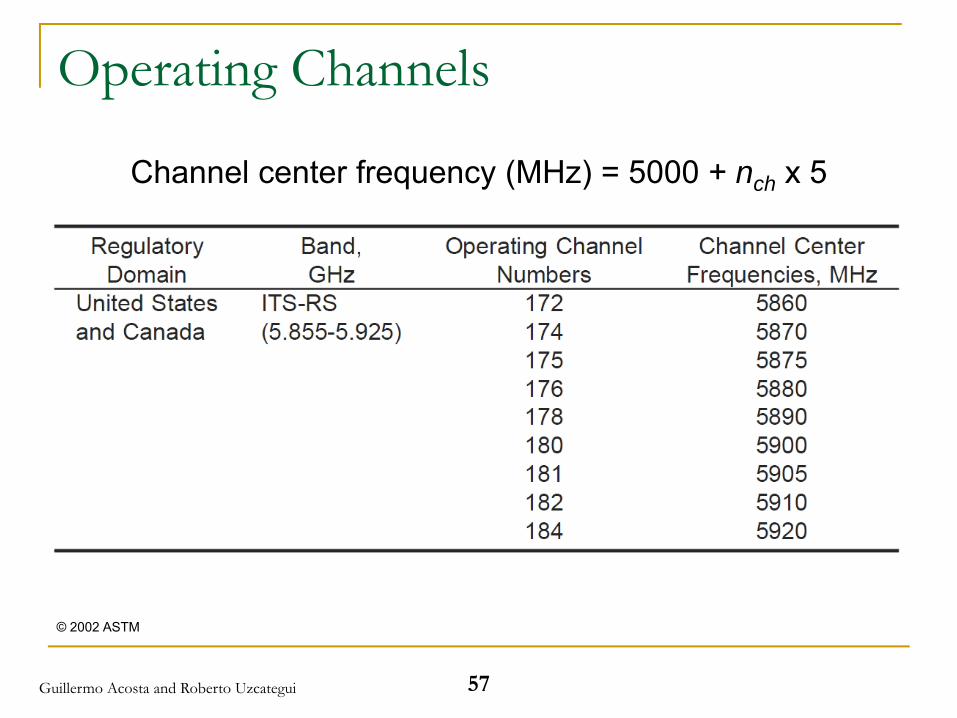
Operating Channels
Channel center frequency (MHz) = 5000 + nch x 5
© 2002 ASTM
57Guillermo Acosta and Roberto Uzcategui
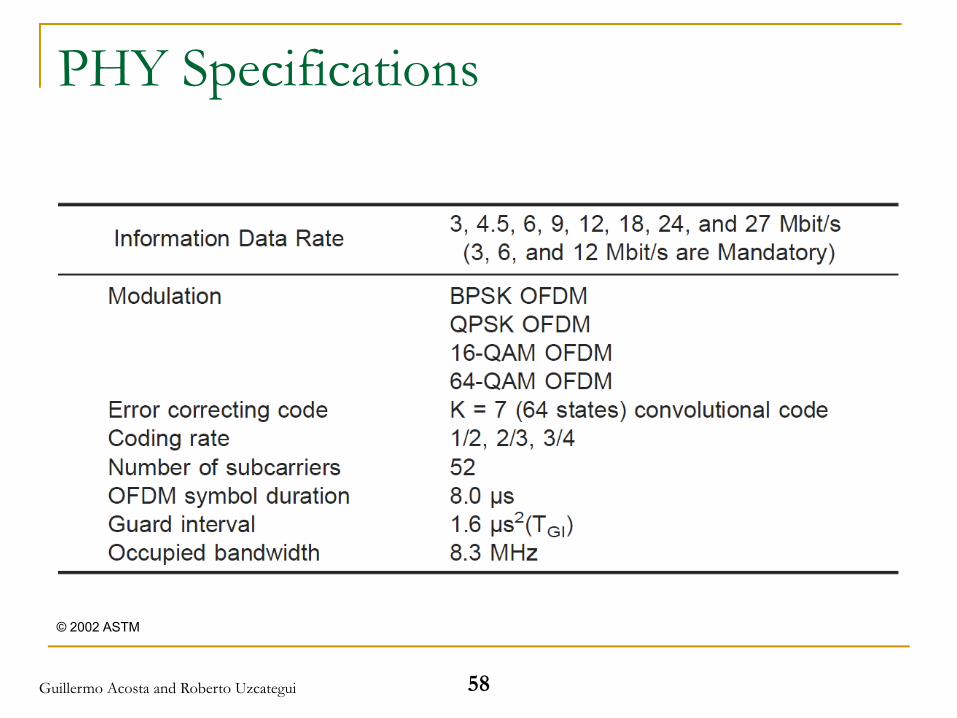
PHY Specifications
© 2002 ASTM
58Guillermo Acosta and Roberto Uzcategui
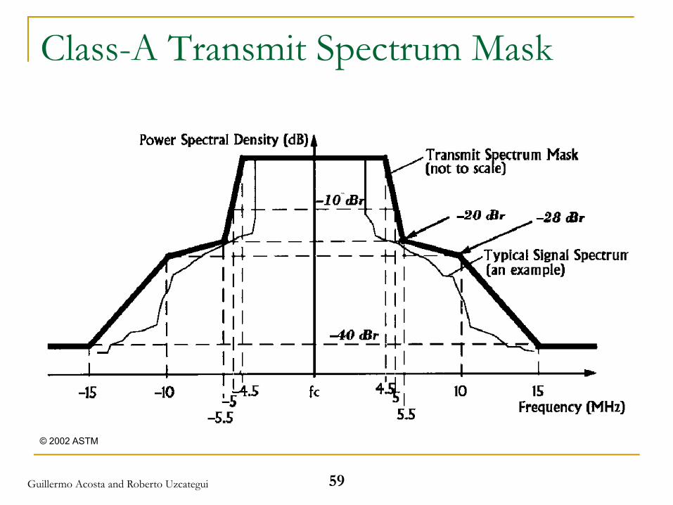
Class-A Transmit Spectrum Mask
© 2002 ASTM
59Guillermo Acosta and Roberto Uzcategui
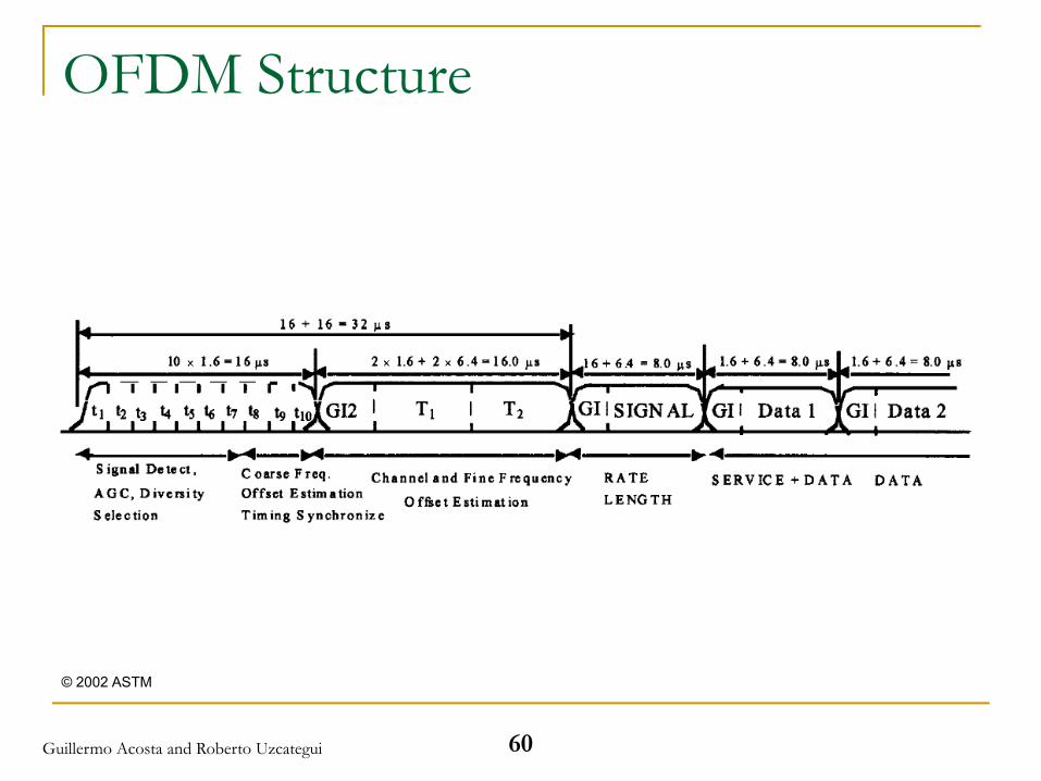
OFDM Structure
© 2002 ASTM
60Guillermo Acosta and Roberto Uzcategui
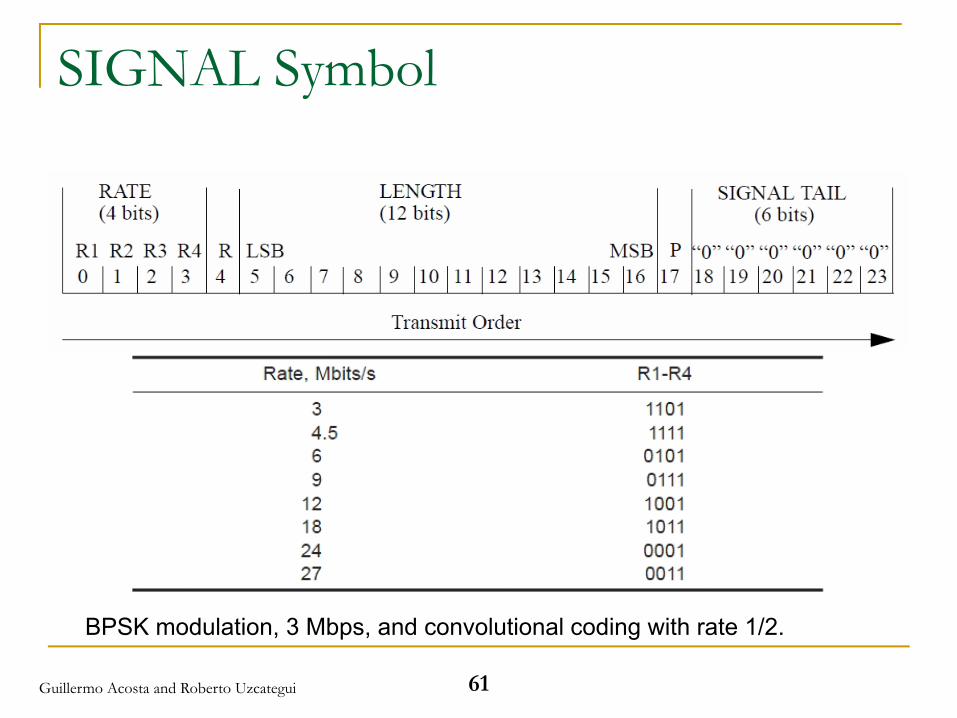
SIGNAL Symbol
BPSK modulation, 3 Mbps, and convolutional coding with rate 1/2.
61Guillermo Acosta and Roberto Uzcategui
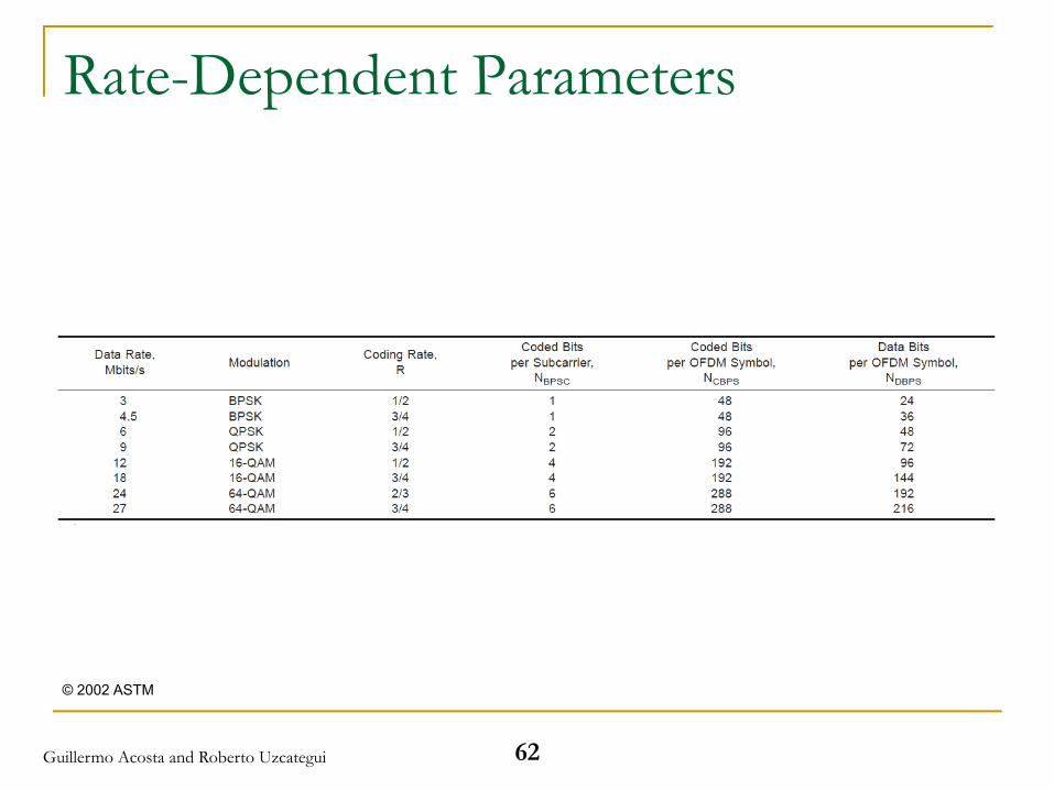
Rate-Dependent Parameters
© 2002 ASTM
62Guillermo Acosta and Roberto Uzcategui
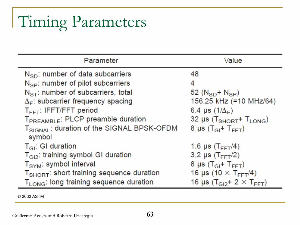
Timing Parameters
© 2002 ASTM
63Guillermo Acosta and Roberto Uzcategui
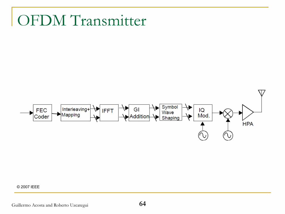
OFDM Transmitter
© 2007 IEEE
64Guillermo Acosta and Roberto Uzcategui
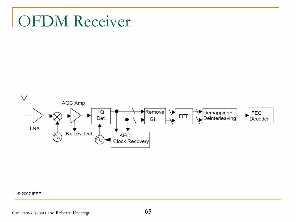
OFDM Receiver
© 2007 IEEE
65Guillermo Acosta and Roberto Uzcategui
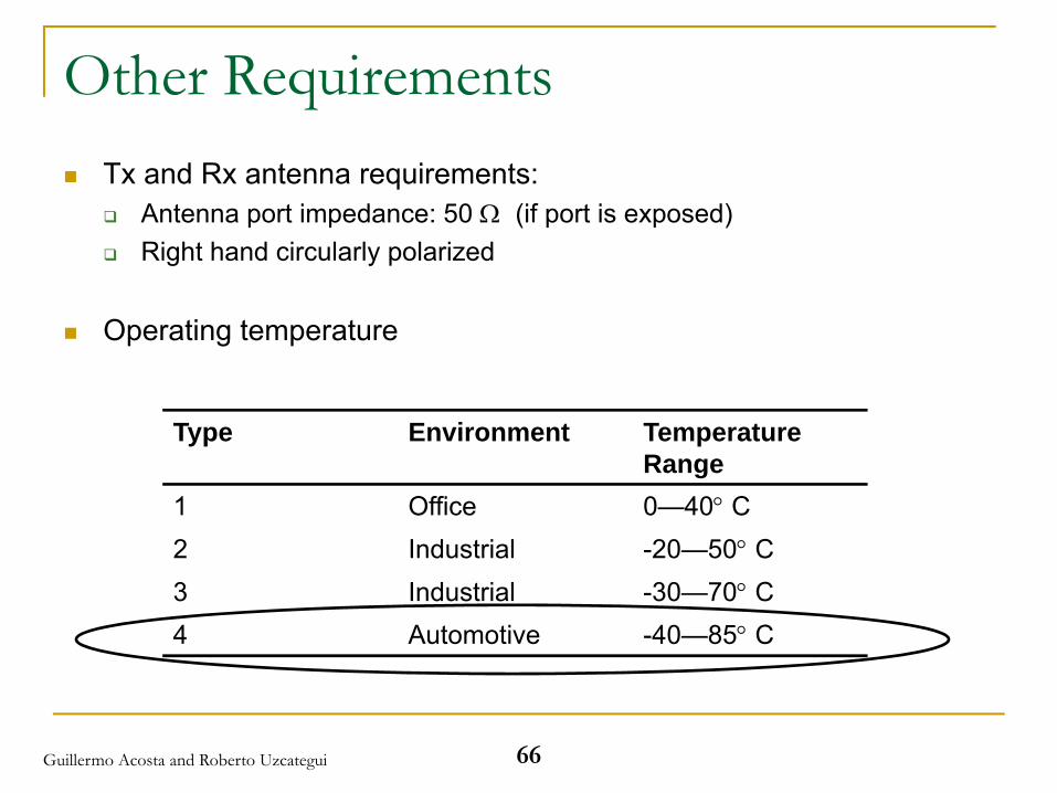
Other RequirementsTx and Rx antenna requirements:
Antenna port impedance: 50 Ω (if port is exposed)Right hand circularly polarized
Operating temperature
Type Environment TemperatureRange
1 Office 0—40° C 2 Industrial -20—50° C3 Industrial -30—70° C4 Automotive -40—85° C
66Guillermo Acosta and Roberto Uzcategui
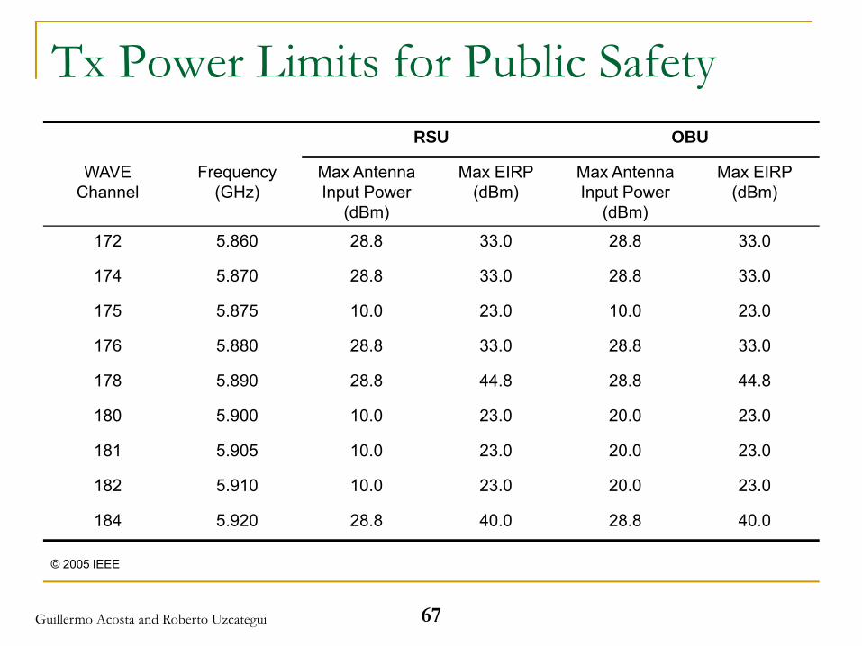
Tx Power Limits for Public Safety
© 2005 IEEE
RSU OBU
WAVEChannel
Frequency(GHz)
Max Antenna Input Power
(dBm)
Max EIRP(dBm)
Max Antenna Input Power
(dBm)
Max EIRP(dBm)
172 5.860 28.8 33.0 28.8 33.0
174 5.870 28.8 33.0 28.8 33.0
175 5.875 10.0 23.0 10.0 23.0
176 5.880 28.8 33.0 28.8 33.0
178 5.890 28.8 44.8 28.8 44.8
180 5.900 10.0 23.0 20.0 23.0
181 5.905 10.0 23.0 20.0 23.0
182 5.910 10.0 23.0 20.0 23.0
184 5.920 28.8 40.0 28.8 40.0
67Guillermo Acosta and Roberto Uzcategui

Tx Power Limits for Private Usage
© 2005 IEEE
RSU OBU
WAVEChannel
Frequency(GHz)
Max Antenna Input Power
(dBm)
Max EIRP(dBm)
Max Antenna Input Power
(dBm)
Max EIRP(dBm)
172 5.860 28.8 33.0 28.8 33.0
174 5.870 28.8 33.0 28.8 33.0
175 5.875 10.0 23.0 10.0 23.0
176 5.880 28.8 33.0 28.8 33.0
178 5.890 28.8 33.0 28.8 33.0
180 5.900 10.0 23.0 20.0 23.0
181 5.905 10.0 23.0 20.0 23.0
182 5.910 10.0 23.0 20.0 23.0
184 5.920 28.8 33.0 28.8 33.0
68Guillermo Acosta and Roberto Uzcategui
Certification
69Guillermo Acosta and Roberto Uzcategui
OmniAirOmni: Open Mobile Network Interoperability
Non-profit trade association
Established in 2003
An alliance of DSRC system manufacturers, operators, integrators, application service providers and others
Mission: To foster and promote the deployment of interoperable 5.9 GHz DSRC systems through the member-defined OmniAirCertification Program
70Guillermo Acosta and Roberto Uzcategui
Wireless Channel
71Guillermo Acosta and Roberto Uzcategui
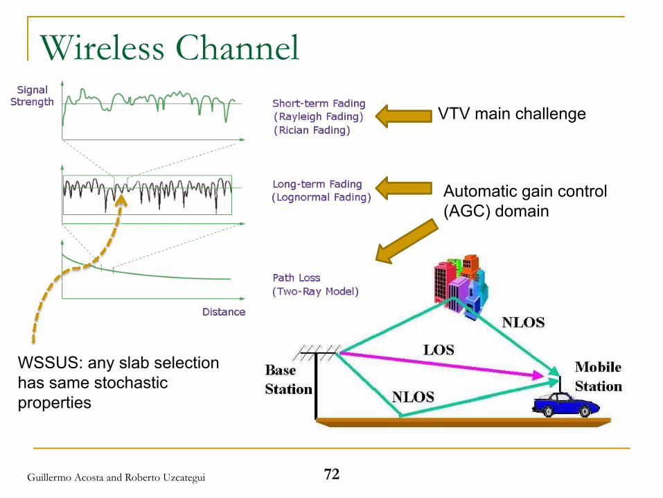
Wireless ChannelVTV main challenge
Automatic gain control (AGC) domain
WSSUS: any slab selection has same stochastic properties
72Guillermo Acosta and Roberto Uzcategui
73
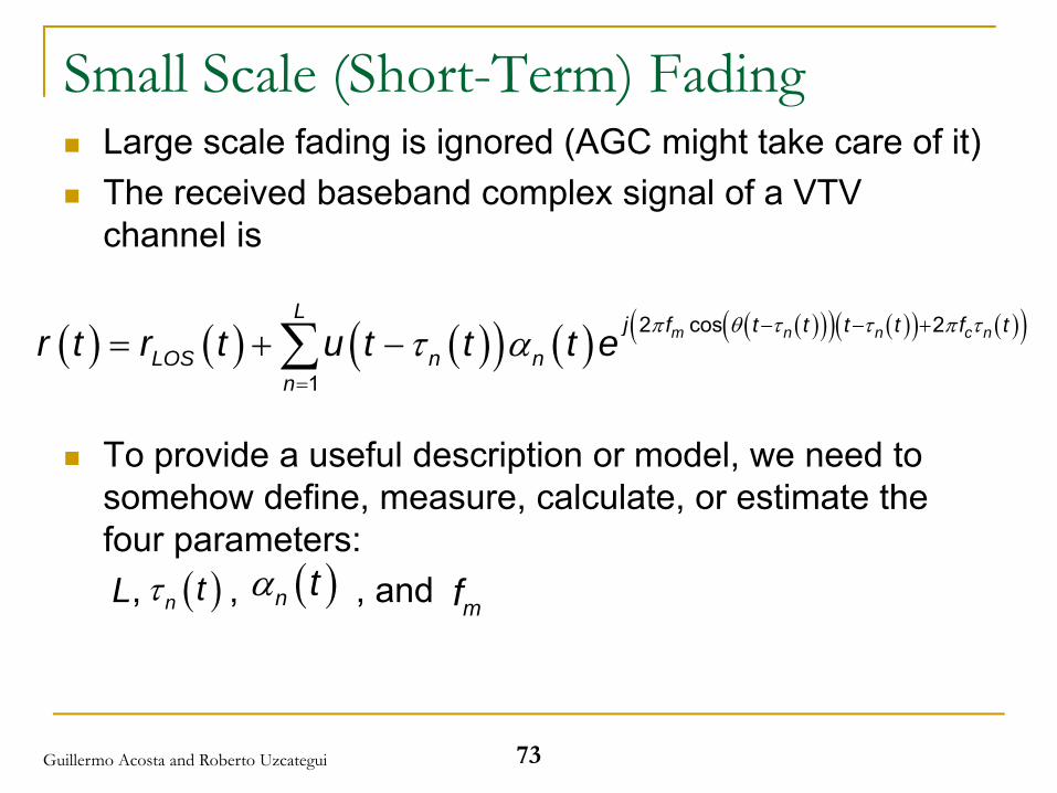
Small Scale (Short-Term) FadingLarge scale fading is ignored (AGC might take care of it)The received baseband complex signal of a VTV channel is
To provide a useful description or model, we need to somehow define, measure, calculate, or estimate the four parameters: L, , , and
( ) ( ) ( )( ) ( ) ( )( )( ) ( )( ) ( )( )π θ τ τ π ττ α
− − +
=
= + −∑ 2 cos 2
1
m n n c nL j f t t t t f t
LOS n nn
r t r t u t t t e
( )n tτ ( )n tαmf
Guillermo Acosta and Roberto Uzcategui
74
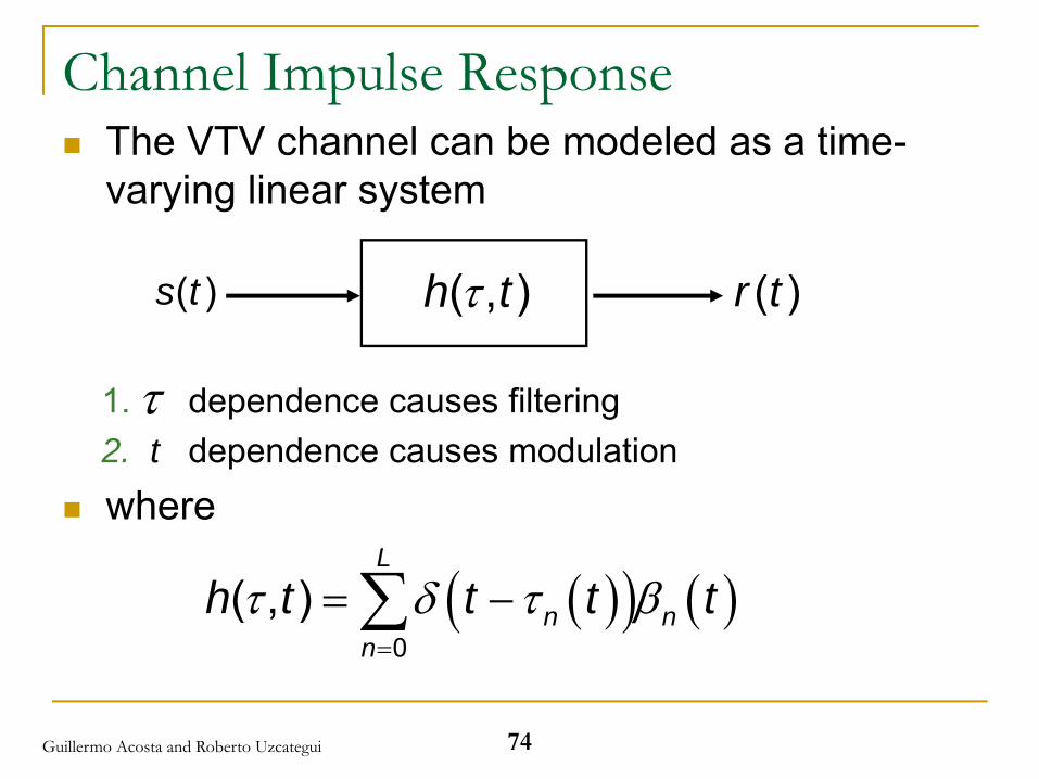
Channel Impulse ResponseThe VTV channel can be modeled as a time-varying linear system
1. dependence causes filtering2. t dependence causes modulationwhere
τ
( )( ) ( )0
( , )L
n nn
h t t t tτ δ τ β=
= −∑
( , )h tτ( )s t ( )r t
Guillermo Acosta and Roberto Uzcategui
Wireless Models
75Guillermo Acosta and Roberto Uzcategui
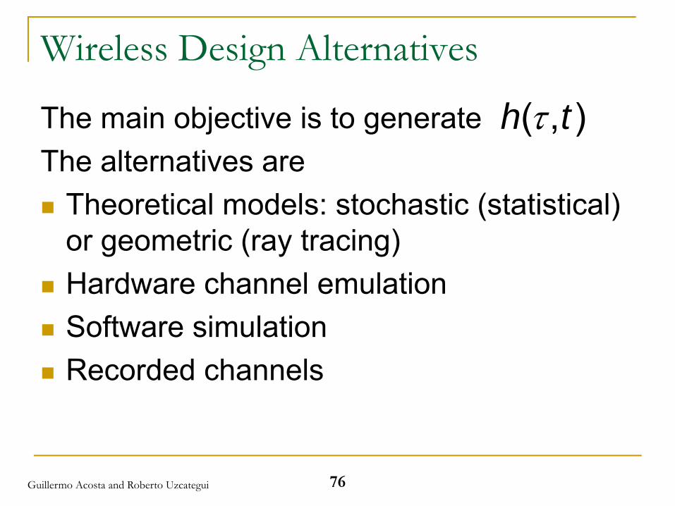
Wireless Design Alternatives
The main objective is to generate The alternatives are
Theoretical models: stochastic (statistical) or geometric (ray tracing)Hardware channel emulationSoftware simulationRecorded channels
( , )h tτ
76Guillermo Acosta and Roberto Uzcategui
77
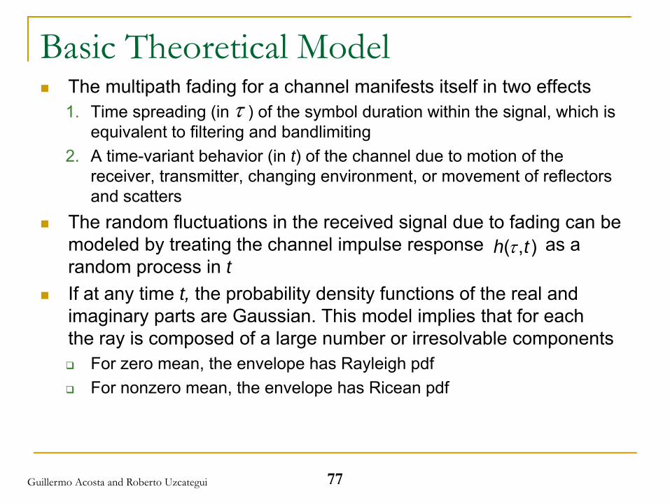
Basic Theoretical ModelThe multipath fading for a channel manifests itself in two effects1. Time spreading (in ) of the symbol duration within the signal, which is
equivalent to filtering and bandlimiting2. A time-variant behavior (in t) of the channel due to motion of the
receiver, transmitter, changing environment, or movement of reflectors and scatters
The random fluctuations in the received signal due to fading can be modeled by treating the channel impulse response as a random process in tIf at any time t, the probability density functions of the real and imaginary parts are Gaussian. This model implies that for each the ray is composed of a large number or irresolvable components
For zero mean, the envelope has Rayleigh pdfFor nonzero mean, the envelope has Ricean pdf
τ
( , )h tτ
Guillermo Acosta and Roberto Uzcategui
78
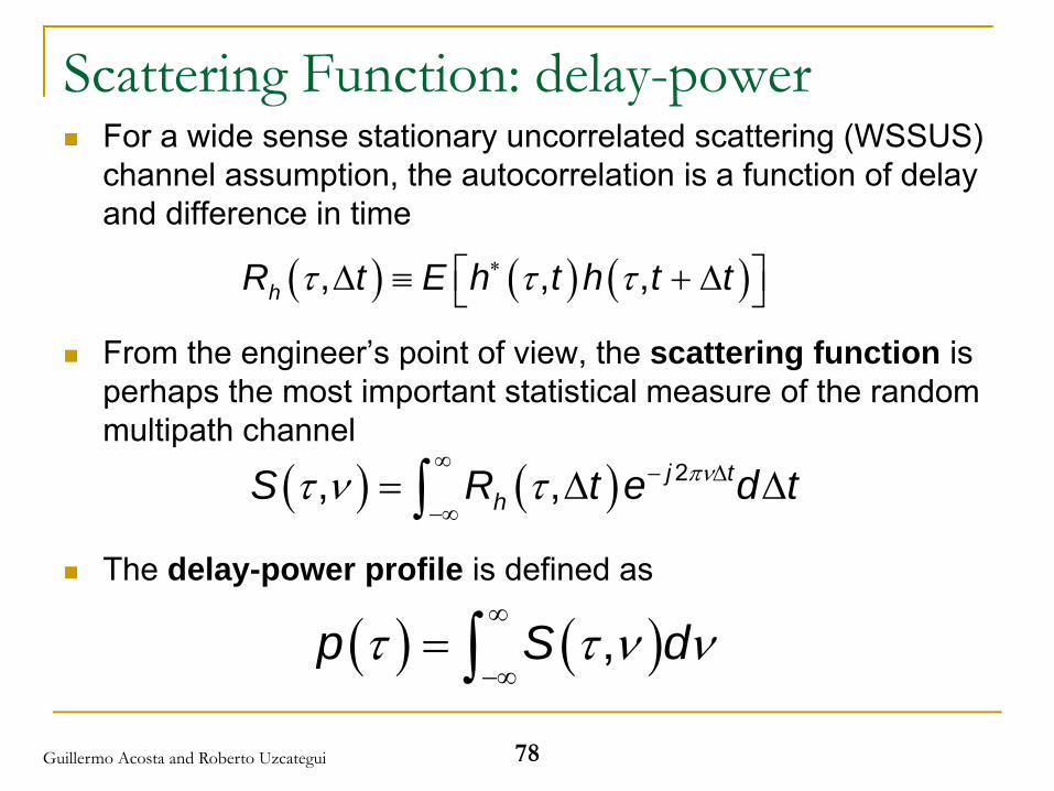
Scattering Function: delay-powerFor a wide sense stationary uncorrelated scattering (WSSUS) channel assumption, the autocorrelation is a function of delay and difference in time
From the engineer’s point of view, the scattering function is perhaps the most important statistical measure of the random multipath channel
The delay-power profile is defined as
( ) ( ) ( )τ τ τ∗⎡ ⎤Δ ≡ + Δ⎣ ⎦, , ,hR t E h t h t t
( ) ( ) πντ ν τ∞ − Δ
−∞= Δ Δ∫ 2, , j t
hS R t e d t
( ) ( )τ τ ν ν∞
−∞= ∫ ,p S d
Guillermo Acosta and Roberto Uzcategui
79
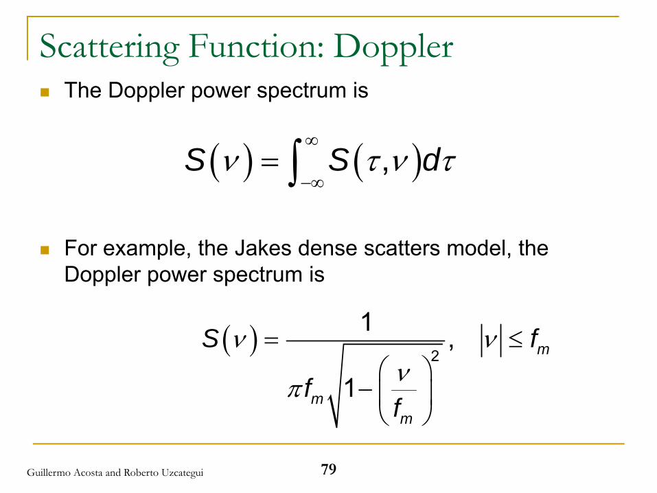
Scattering Function: DopplerThe Doppler power spectrum is
For example, the Jakes dense scatters model, the Doppler power spectrum is
( ) ( )ν τ ν τ∞
−∞= ∫ ,S S d
( )ν ννπ
= ≤⎛ ⎞
− ⎜ ⎟⎝ ⎠
2
1 ,
1m
mm
S f
ff
Guillermo Acosta and Roberto Uzcategui
80
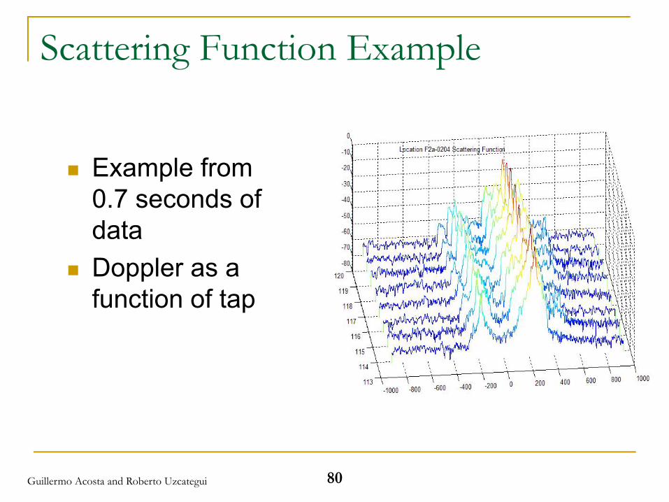
Scattering Function Example
Example from 0.7 seconds of dataDoppler as a function of tap
Guillermo Acosta and Roberto Uzcategui
81
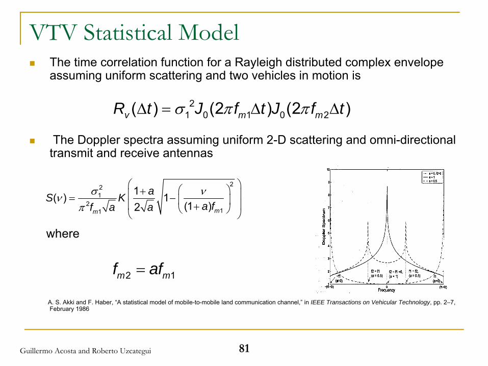
VTV Statistical ModelThe time correlation function for a Rayleigh distributed complex envelope assuming uniform scattering and two vehicles in motion is
The Doppler spectra assuming uniform 2-D scattering and omni-directional transmit and receive antennas
where
A. S. Akki and F. Haber, “A statistical model of mobile-to-mobile land communication channel,” in IEEE Transactions on Vehicular Technology, pp. 2–7, February 1986
21 0 1 0 2( ) (2 ) (2 )v m mR t J f t J f tσ π πΔ = Δ Δ
221
211
1( ) 1(1 )2 mm
aS Ka ff a a
σ ννπ
⎛ ⎞⎛ ⎞+⎜ ⎟= − ⎜ ⎟⎜ ⎟+⎝ ⎠⎝ ⎠
2 1m mf af=
Guillermo Acosta and Roberto Uzcategui
82
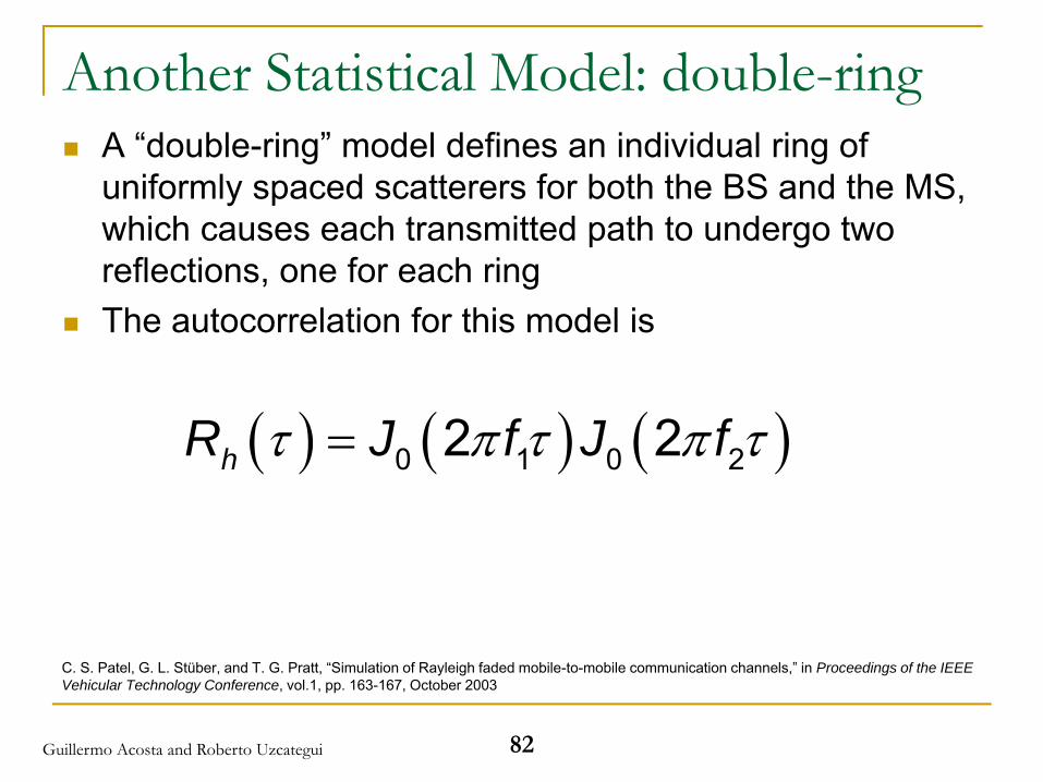
Another Statistical Model: double-ringA “double-ring” model defines an individual ring of uniformly spaced scatterers for both the BS and the MS, which causes each transmitted path to undergo two reflections, one for each ring The autocorrelation for this model is
C. S. Patel, G. L. Stüber, and T. G. Pratt, “Simulation of Rayleigh faded mobile-to-mobile communication channels,” in Proceedings of the IEEE Vehicular Technology Conference, vol.1, pp. 163-167, October 2003
( ) ( ) ( )τ π τ π τ= 0 1 0 22 2hR J f J f
Guillermo Acosta and Roberto Uzcategui
What to Do with or How to Use the Theoretical Models?
We need to remember that the models derivations assume stochastic processes such as uniform distribution of scatters or normal probability densities in their amplitude variationsThere are plenty of random sources available that we can use to generate signals that behave as the theoretical modelsOnce we have this signals, we use them to amplitude modulate the transmitted signal, i.e., we generate the
( )n tβ
83Guillermo Acosta and Roberto Uzcategui
84
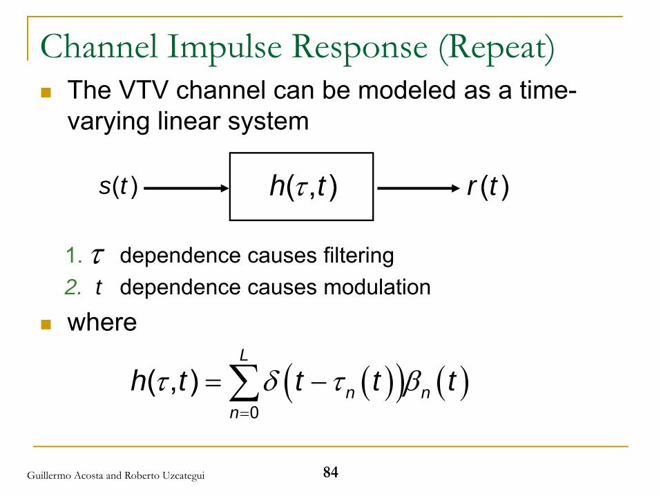
Channel Impulse Response (Repeat)The VTV channel can be modeled as a time-varying linear system
1. dependence causes filtering2. t dependence causes modulationwhere
τ
( )( ) ( )0
( , )L
n nn
h t t t tτ δ τ β=
= −∑
( , )h tτ( )s t ( )r t
Guillermo Acosta and Roberto Uzcategui
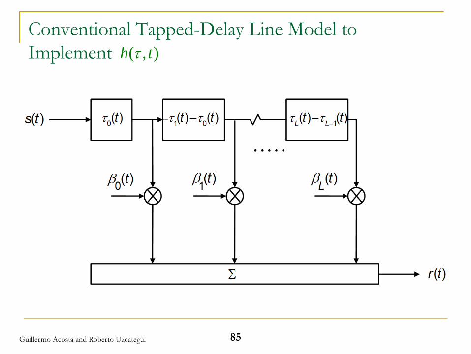
85
Conventional Tapped-Delay Line Model to Implement ( , )h tτ
Guillermo Acosta and Roberto Uzcategui
86
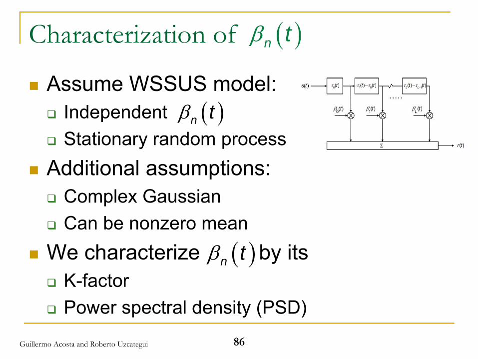
Characterization of
Assume WSSUS model:Independent Stationary random process
Additional assumptions:Complex Gaussian Can be nonzero mean
We characterize by itsK-factor Power spectral density (PSD)
( )n tβ
( )n tβ
( )n tβ
Guillermo Acosta and Roberto Uzcategui
Wireless Design Alternatives
87Guillermo Acosta and Roberto Uzcategui
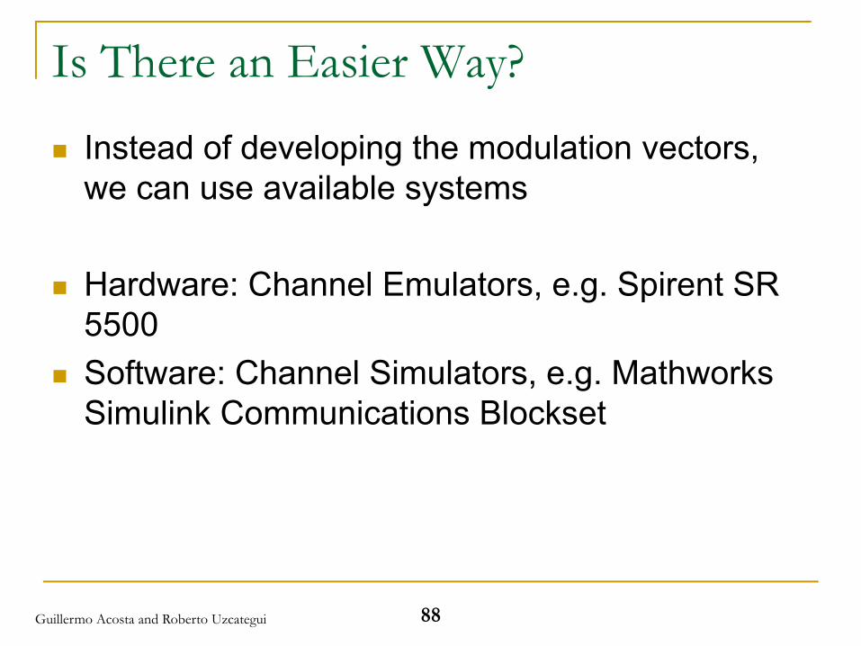
Is There an Easier Way?
Instead of developing the modulation vectors, we can use available systems
Hardware: Channel Emulators, e.g. Spirent SR 5500Software: Channel Simulators, e.g. MathworksSimulink Communications Blockset
88Guillermo Acosta and Roberto Uzcategui

89
Channel Emulator
A channel emulator is a device or machine that “replaces” a real channel for laboratory testingCertification tests are performed using channel emulators
Guillermo Acosta and Roberto Uzcategui
90
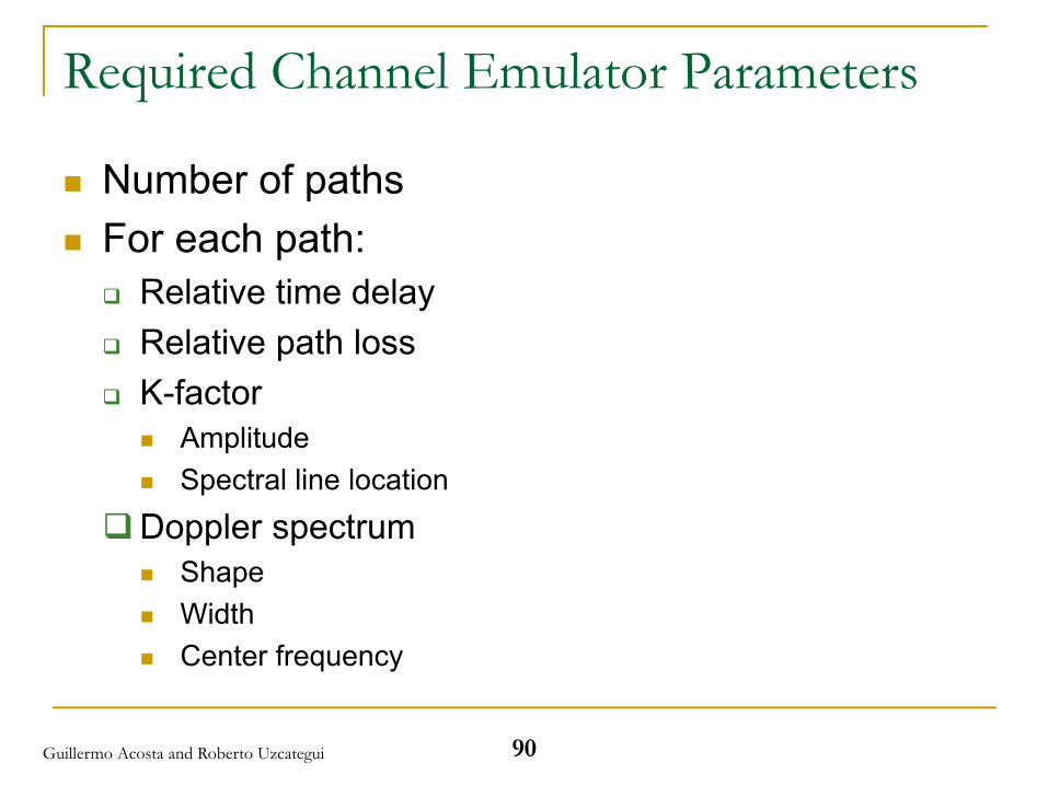
Required Channel Emulator Parameters
Number of pathsFor each path:
Relative time delayRelative path lossK-factor
AmplitudeSpectral line location
Doppler spectrumShapeWidthCenter frequency
Guillermo Acosta and Roberto Uzcategui
91
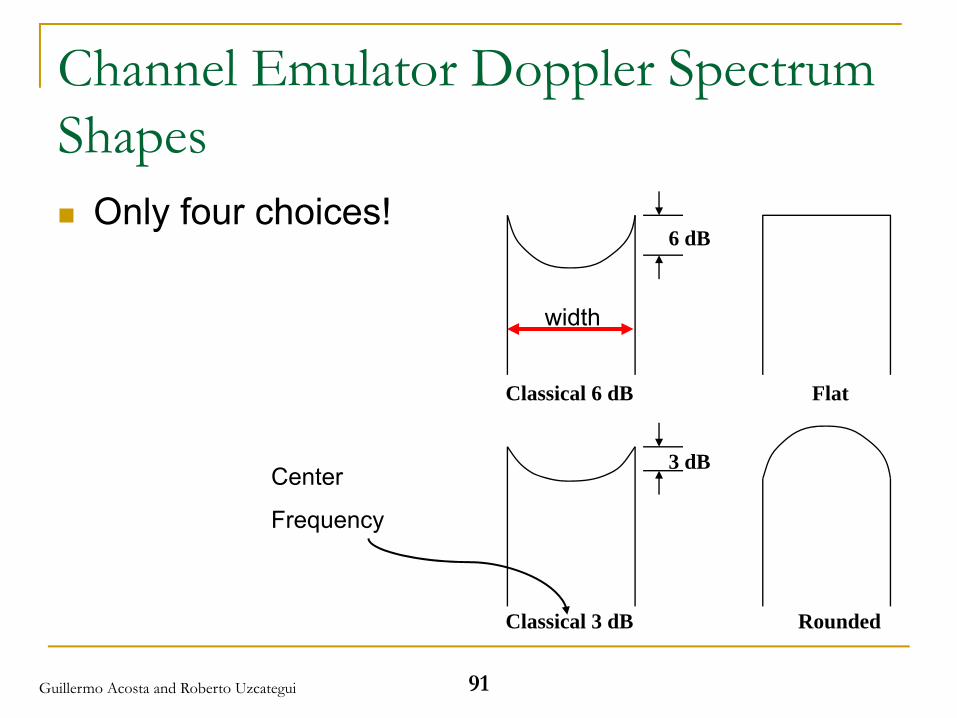
Channel Emulator Doppler Spectrum Shapes
Only four choices!6 dB
Classical 6 dB
3 dB
Classical 3 dB Rounded
Flat
width
Center
Frequency
Guillermo Acosta and Roberto Uzcategui
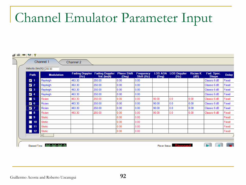
92
Channel Emulator Parameter Input
Guillermo Acosta and Roberto Uzcategui
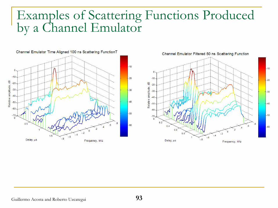
93
Examples of Scattering Functions Produced by a Channel Emulator
Guillermo Acosta and Roberto Uzcategui
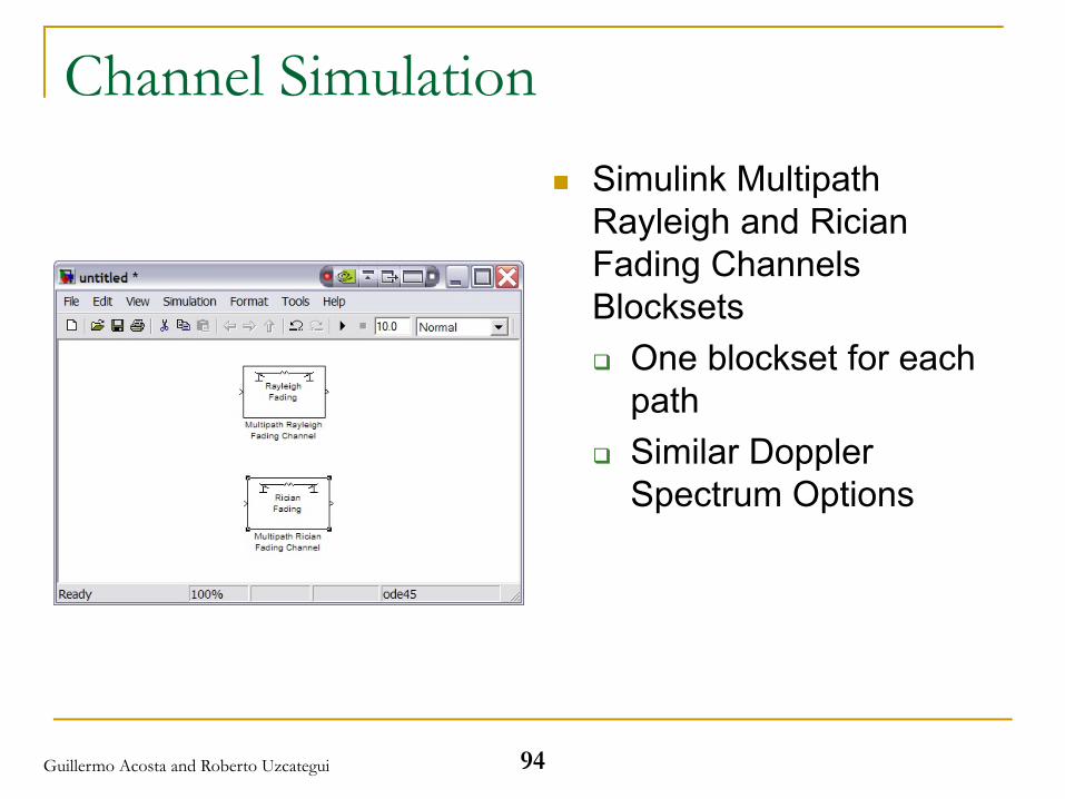
Channel SimulationSimulink Multipath Rayleigh and RicianFading Channels Blocksets
One blockset for each pathSimilar Doppler Spectrum Options
94Guillermo Acosta and Roberto Uzcategui
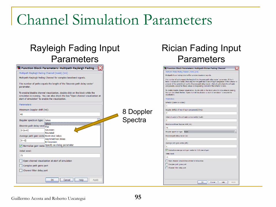
Channel Simulation Parameters
Rayleigh Fading Input Parameters
Rician Fading Input Parameters
8 Doppler Spectra
95Guillermo Acosta and Roberto Uzcategui
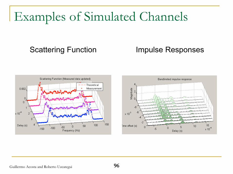
Examples of Simulated Channels
Scattering Function Impulse Responses
96Guillermo Acosta and Roberto Uzcategui
Wireless Channel Sounding
97Guillermo Acosta and Roberto Uzcategui
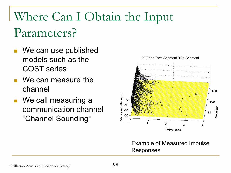
Where Can I Obtain the Input Parameters?
We can use published models such as the COST seriesWe can measure the channelWe call measuring a communication channel “Channel Sounding”
Example of Measured Impulse Responses
98Guillermo Acosta and Roberto Uzcategui
99
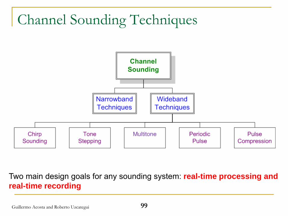
Channel Sounding Techniques
Two main design goals for any sounding system: real-time processing and real-time recording
Guillermo Acosta and Roberto Uzcategui
100
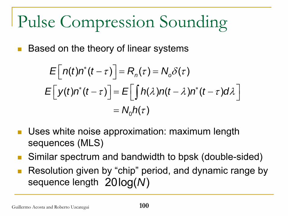
Pulse Compression SoundingBased on the theory of linear systems
Uses white noise approximation: maximum length sequences (MLS)Similar spectrum and bandwidth to bpsk (double-sided)Resolution given by “chip” period, and dynamic range by sequence length
τ λ λ τ λ
τ
∗ ∗⎡ ⎤⎡ ⎤− = − −⎣ ⎦ ⎣ ⎦=
∫0
( ) ( ) ( ) ( ) ( )
( )
E y t n t E h n t n t d
N h
20log( )N
τ τ δ τ∗⎡ ⎤− = =⎣ ⎦( ) ( ) ( ) ( )n oE n t n t R N
Guillermo Acosta and Roberto Uzcategui
101
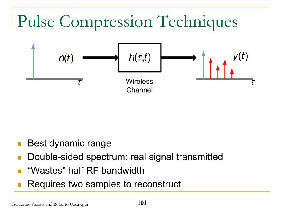
Pulse Compression Techniques
Best dynamic rangeDouble-sided spectrum: real signal transmitted“Wastes” half RF bandwidthRequires two samples to reconstruct
Guillermo Acosta and Roberto Uzcategui
102
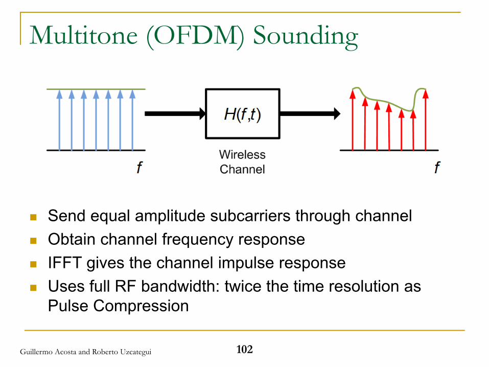
Multitone (OFDM) Sounding
Send equal amplitude subcarriers through channelObtain channel frequency responseIFFT gives the channel impulse responseUses full RF bandwidth: twice the time resolution as Pulse Compression
Guillermo Acosta and Roberto Uzcategui
103
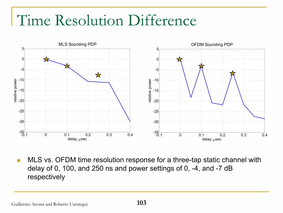
Time Resolution Difference
MLS vs. OFDM time resolution response for a three-tap static channel with delay of 0, 100, and 250 ns and power settings of 0, -4, and -7 dB respectively
-0.1 0 0.1 0.2 0.3 0.4-35
-30
-25
-20
-15
-10
-5
0
5MLS Sounding PDP
rela
tive
pow
er
delay, μsec-0.1 0 0.1 0.2 0.3 0.4
-35
-30
-25
-20
-15
-10
-5
0
5OFDM Sounding PDP
rela
tive
pow
er
delay, μsec
Guillermo Acosta and Roberto Uzcategui
104
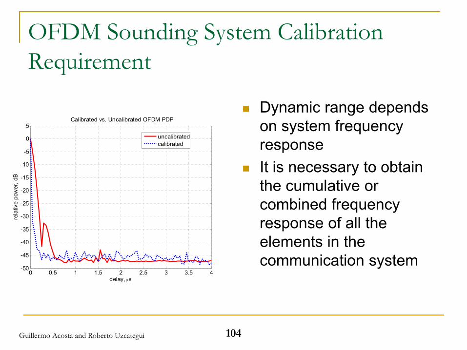
OFDM Sounding System Calibration Requirement
Dynamic range depends on system frequency responseIt is necessary to obtain the cumulative or combined frequency response of all the elements in the communication system
0 0.5 1 1.5 2 2.5 3 3.5 4-50
-45
-40
-35
-30
-25
-20
-15
-10
-5
0
5
delay, μs
rela
tive
pow
er, d
B
Calibrated vs. Uncalibrated OFDM PDP
uncalibratedcalibrated
Guillermo Acosta and Roberto Uzcategui
105
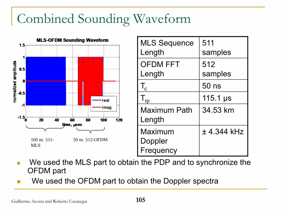
Combined Sounding Waveform
We used the MLS part to obtain the PDP and to synchronize the OFDM partWe used the OFDM part to obtain the Doppler spectra
100 ns 511-MLS
50 ns 512-OFDM
MLS Sequence Length
511 samples
OFDM FFT Length
512 samples
Tc 50 nsTrp 115.1 μsMaximum Path Length
34.53 km
Maximum Doppler Frequency
± 4.344 kHz
Guillermo Acosta and Roberto Uzcategui
How Do We Design a Channel Sounder?
If our objective is to sound a channel to generate a channel model, we focus on real-time recording for post processingWe can use a software radio based architectureThe design objective is to record In-Phase and Quadrature (I/Q) baseband samples for post-processingThe Analog-to-Digital (ADC) and Digital-to-Analog (DAC) converters are the defining elements
106Guillermo Acosta and Roberto Uzcategui
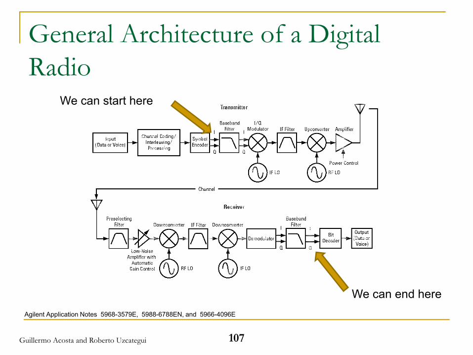
General Architecture of a Digital Radio
We can start here
We can end hereAgilent Application Notes 5968-3579E, 5988-6788EN, and 5966-4096E
107Guillermo Acosta and Roberto Uzcategui
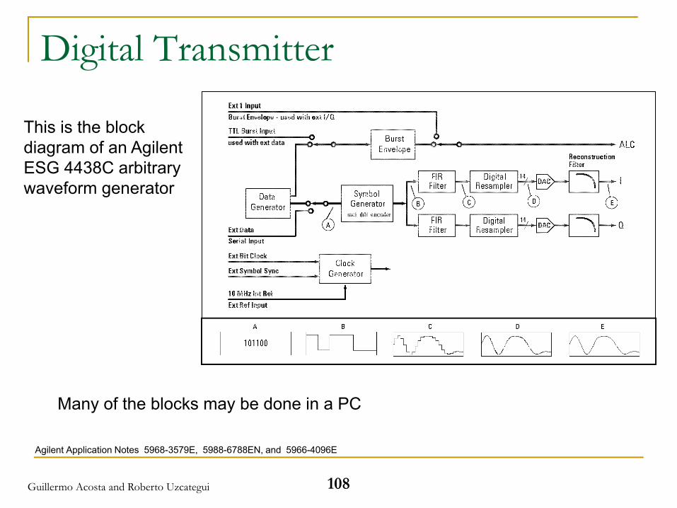
Digital Transmitter
Agilent Application Notes 5968-3579E, 5988-6788EN, and 5966-4096E
This is the block diagram of an Agilent ESG 4438C arbitrary waveform generator
Many of the blocks may be done in a PC
108Guillermo Acosta and Roberto Uzcategui
109
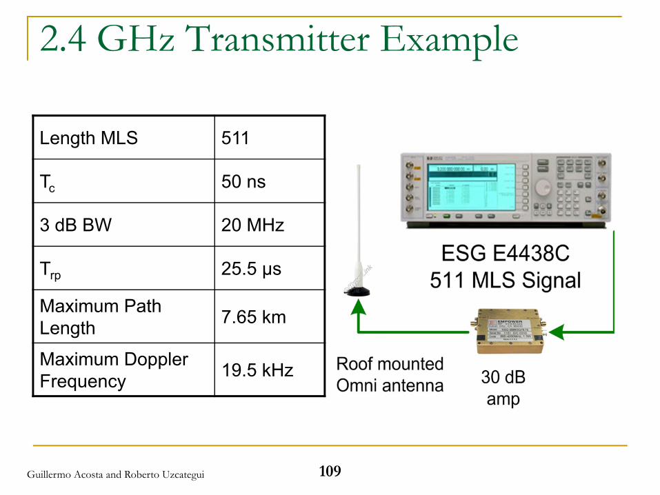
2.4 GHz Transmitter Example
Length MLS 511
Tc 50 ns
3 dB BW 20 MHz
Trp 25.5 µs
Maximum Path Length 7.65 km
Maximum Doppler Frequency 19.5 kHz
Guillermo Acosta and Roberto Uzcategui
110
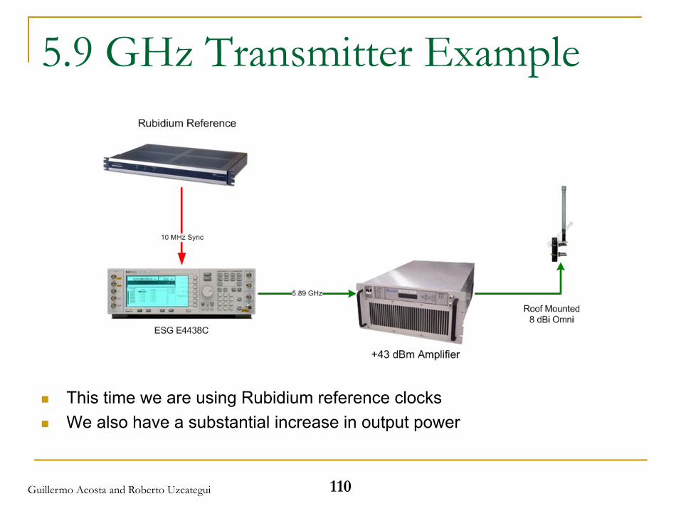
5.9 GHz Transmitter Example
This time we are using Rubidium reference clocksWe also have a substantial increase in output power
Guillermo Acosta and Roberto Uzcategui
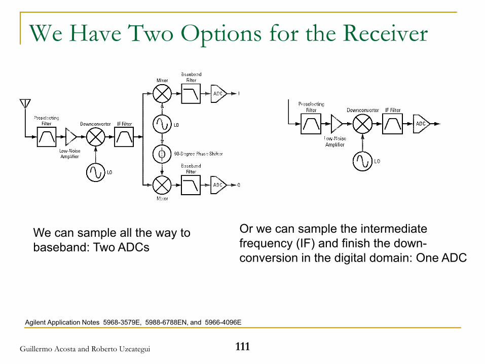
We Have Two Options for the Receiver
Agilent Application Notes 5968-3579E, 5988-6788EN, and 5966-4096E
We can sample all the way to baseband: Two ADCs
Or we can sample the intermediate frequency (IF) and finish the down-conversion in the digital domain: One ADC
111Guillermo Acosta and Roberto Uzcategui
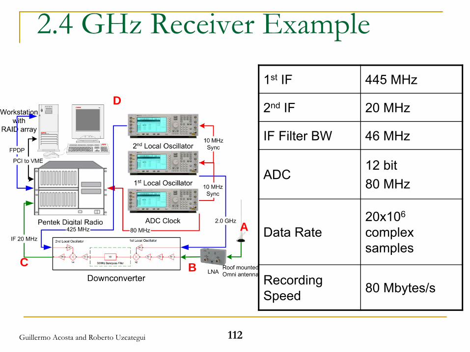
112
2.4 GHz Receiver Example
1st IF 445 MHz
2nd IF 20 MHz
IF Filter BW 46 MHz
ADC12 bit 80 MHz
Data Rate20x106
complex samples
Recording Speed 80 Mbytes/s
B
A
C
D
Guillermo Acosta and Roberto Uzcategui
113
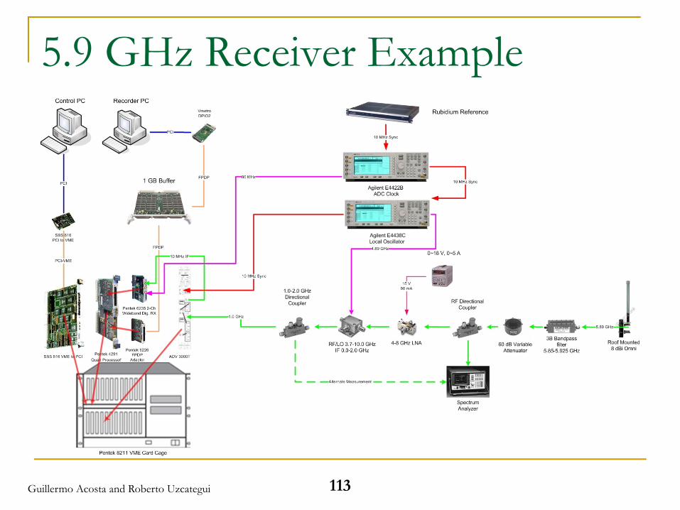
5.9 GHz Receiver Example
Guillermo Acosta and Roberto Uzcategui
Today’s Technology
RecordingSince the introduction of the PCI-E bus, direct to hard drive recording speed keeps increasingThe latest specification for a RAID system is 1.2 GB/s (300 Mega complex samples per second [four bytes]) and up to 512 TBAssuming that we use the four bytes per complex sample, we can sound 300 MHz RF bandwidth for a time resolution of 3.33 ns
ADCTexas Instruments ADS5474 is a 400 MSPS 14 bit ADC
114Guillermo Acosta and Roberto Uzcategui
“Off the Shelf” Systems
National Instruments NI PXIe-5663: 16-bit, 150 MS/s“Affordable” Option: Ettus USRP2 software radio system with two 100 MS/s 14-bit ADCPentek RTS 2701: two 125 MS/s 14-bit ADC
115Guillermo Acosta and Roberto Uzcategui
Wireless Channel Model Development
116Guillermo Acosta and Roberto Uzcategui
Post Processing Examples
We will use the next slides to show examples of the type of information you can obtain from the recorded I/Q samples We should recall that our objective is to create a useful channel model, i.e., a model to use with the emulator or simulatorWe finish this section with an example of a finished product
117Guillermo Acosta and Roberto Uzcategui
118
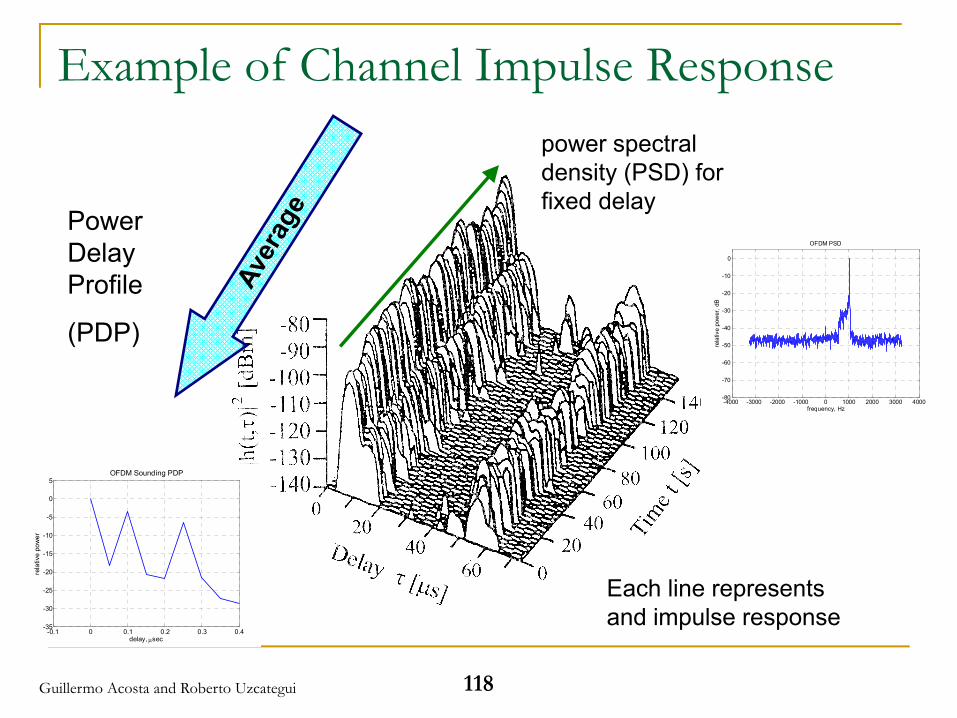
Example of Channel Impulse Response
Power Delay Profile
(PDP)
power spectral density (PSD) for fixed delay
Each line represents and impulse response
-4000 -3000 -2000 -1000 0 1000 2000 3000 4000-80
-70
-60
-50
-40
-30
-20
-10
0
frequency, Hz
rela
tive
pow
er, d
B
OFDM PSD
-0.1 0 0.1 0.2 0.3 0.4-35
-30
-25
-20
-15
-10
-5
0
5OFDM Sounding PDP
rela
tive
pow
er
delay, μsec
Guillermo Acosta and Roberto Uzcategui
119
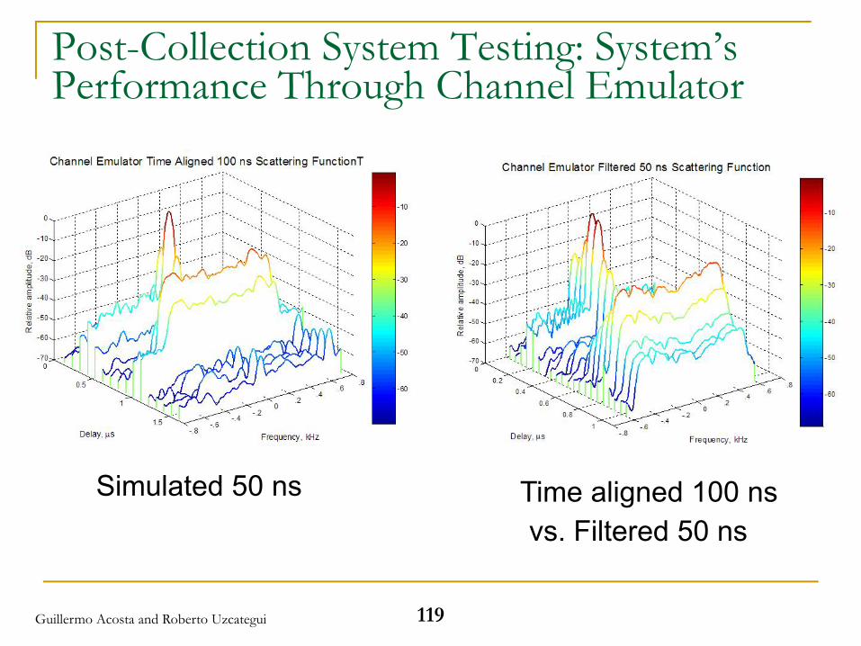
Post-Collection System Testing: System’s Performance Through Channel Emulator
Simulated 50 ns Time aligned 100 ns vs. Filtered 50 ns
Guillermo Acosta and Roberto Uzcategui
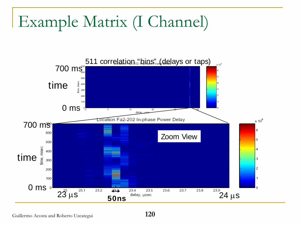
120
Example Matrix (I Channel)
0 ms
700 ms
time
0 ms
700 ms
time
Zoom View
23 μs 24 μs
511 correlation “bins” (delays or taps)
50ns
Guillermo Acosta and Roberto Uzcategui
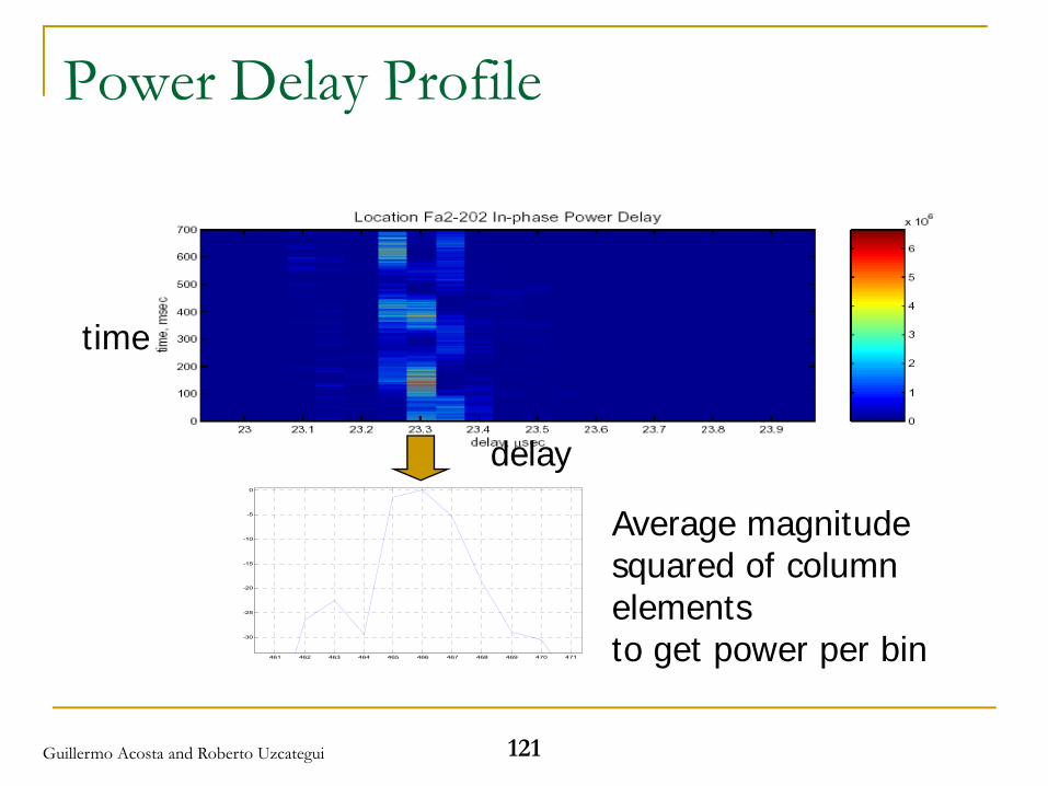
121
Power Delay Profile
461 462 463 464 465 466 467 468 469 470 471
-30
-25
-20
-15
-10
-5
0
Average magnitudesquared of column elementsto get power per bin
time
delay
Guillermo Acosta and Roberto Uzcategui
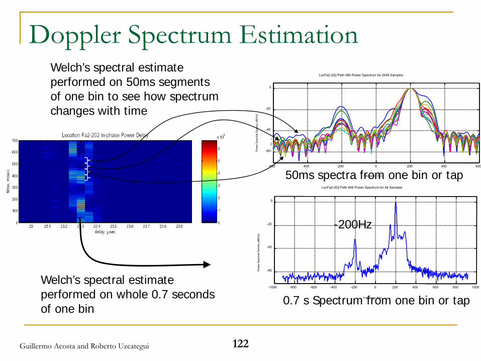
122
Doppler Spectrum Estimation
-600 -400 -200 0 200 400 600
-60
-40
-20
0
Pow
er S
pect
ral D
ensi
ty (d
B/H
z)
Frequency (Hz)
LocFa2-202 Path 466 Power Spectrum for 2048 Samples
-1000 -800 -600 -400 -200 0 200 400 600 800 1000
-60
-40
-20
0
Pow
er S
pect
ral D
ensi
ty (d
B/H
z)
Frequency (Hz)
LocFa2-202 Path 466 Power Spectrum for All Samples
Welch’s spectral estimate performed on whole 0.7 secondsof one bin
0.7 s Spectrum from one bin or tap
Welch’s spectral estimate performed on 50ms segmentsof one bin to see how spectrumchanges with time
50ms spectra from one bin or tap
-200Hz
Guillermo Acosta and Roberto Uzcategui
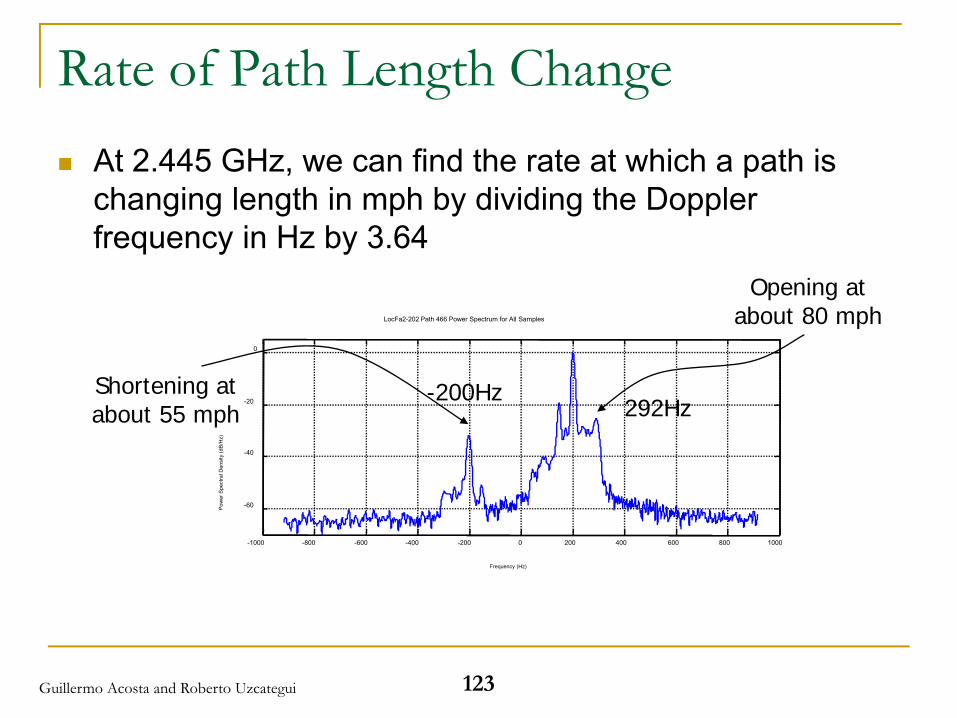
123
Rate of Path Length ChangeAt 2.445 GHz, we can find the rate at which a path is changing length in mph by dividing the Doppler frequency in Hz by 3.64
-1000 -800 -600 -400 -200 0 200 400 600 800 1000
-60
-40
-20
0
Pow
er S
pect
ral D
ensi
ty (d
B/H
z)
Frequency (Hz)
LocFa2-202 Path 466 Power Spectrum for All Samples
-200HzShortening atabout 55 mph 292Hz
Opening atabout 80 mph
Guillermo Acosta and Roberto Uzcategui
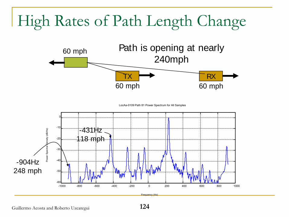
124
High Rates of Path Length Change
-1000 -800 -600 -400 -200 0 200 400 600 800 1000-60
-50
-40
-30
-20
-10
0
Pow
er S
pect
ral D
ensi
ty (d
B/H
z)
Frequency (Hz)
LocAa-0109 Path 81 Power Spectrum for All Samples
-904Hz248 mph
-431Hz118 mph
TX RX
60 mph
60 mph 60 mph
Path is opening at nearly240mph
Guillermo Acosta and Roberto Uzcategui
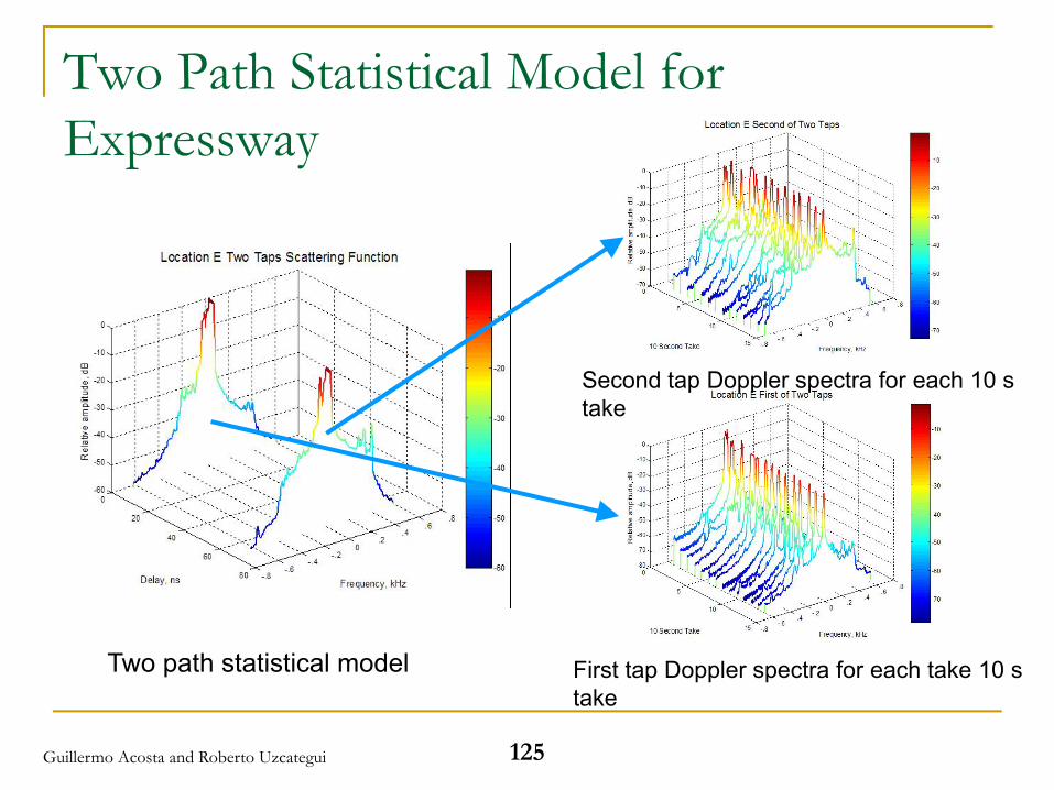
125
Two Path Statistical Model for Expressway
Two path statistical model First tap Doppler spectra for each take 10 stake
Second tap Doppler spectra for each 10 stake
Guillermo Acosta and Roberto Uzcategui
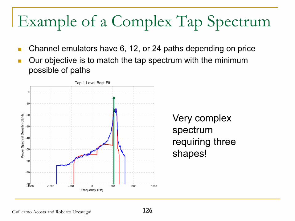
126
Example of a Complex Tap SpectrumChannel emulators have 6, 12, or 24 paths depending on price Our objective is to match the tap spectrum with the minimum possible of paths
-1500 -1000 -500 0 500 1000 1500-80
-70
-60
-50
-40
-30
-20
-10
0
Tap 1 Level Best Fit
Pow
er S
pect
ral D
ensi
ty (d
B/H
z)
Frequency (Hz)
Very complex spectrum requiring three shapes!
Guillermo Acosta and Roberto Uzcategui
127
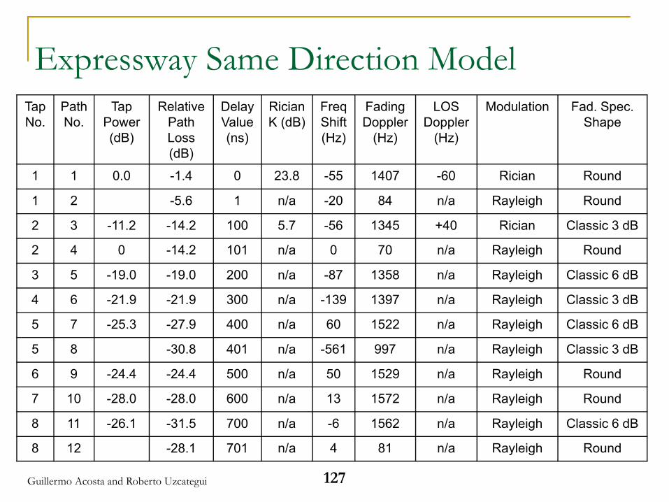
Expressway Same Direction ModelTap No.
Path No.
Tap Power (dB)
Relative Path Loss (dB)
Delay Value (ns)
Rician K (dB)
FreqShift (Hz)
Fading Doppler
(Hz)
LOS Doppler
(Hz)
Modulation Fad. Spec. Shape
1 1 0.0 -1.4 0 23.8 -55 1407 -60 Rician Round
1 2 -5.6 1 n/a -20 84 n/a Rayleigh Round
2 3 -11.2 -14.2 100 5.7 -56 1345 +40 Rician Classic 3 dB
2 4 0 -14.2 101 n/a 0 70 n/a Rayleigh Round
3 5 -19.0 -19.0 200 n/a -87 1358 n/a Rayleigh Classic 6 dB
4 6 -21.9 -21.9 300 n/a -139 1397 n/a Rayleigh Classic 3 dB
5 7 -25.3 -27.9 400 n/a 60 1522 n/a Rayleigh Classic 6 dB
5 8 -30.8 401 n/a -561 997 n/a Rayleigh Classic 3 dB
6 9 -24.4 -24.4 500 n/a 50 1529 n/a Rayleigh Round
7 10 -28.0 -28.0 600 n/a 13 1572 n/a Rayleigh Round
8 11 -26.1 -31.5 700 n/a -6 1562 n/a Rayleigh Classic 6 dB
8 12 -28.1 701 n/a 4 81 n/a Rayleigh Round
Guillermo Acosta and Roberto Uzcategui
128
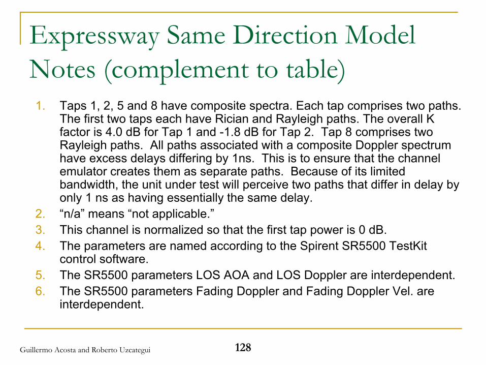
Expressway Same Direction Model Notes (complement to table)1. Taps 1, 2, 5 and 8 have composite spectra. Each tap comprises two paths.
The first two taps each have Rician and Rayleigh paths. The overall K factor is 4.0 dB for Tap 1 and -1.8 dB for Tap 2. Tap 8 comprises two Rayleigh paths. All paths associated with a composite Doppler spectrum have excess delays differing by 1ns. This is to ensure that the channel emulator creates them as separate paths. Because of its limited bandwidth, the unit under test will perceive two paths that differ in delay by only 1 ns as having essentially the same delay.
2. “n/a” means “not applicable.”3. This channel is normalized so that the first tap power is 0 dB.4. The parameters are named according to the Spirent SR5500 TestKit
control software.5. The SR5500 parameters LOS AOA and LOS Doppler are interdependent.6. The SR5500 parameters Fading Doppler and Fading Doppler Vel. are
interdependent.
Guillermo Acosta and Roberto Uzcategui
MIMO Channel Sounding
129Guillermo Acosta and Roberto Uzcategui
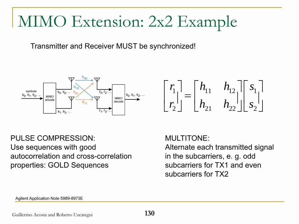
MIMO Extension: 2x2 Example
1 11 12 1
2 21 22 2
r h h sr h h s⎡ ⎤ ⎡ ⎤ ⎡ ⎤
=⎢ ⎥ ⎢ ⎥ ⎢ ⎥⎣ ⎦ ⎣ ⎦ ⎣ ⎦
Agilent Application Note 5989-8973E
PULSE COMPRESSION:Use sequences with good autocorrelation and cross-correlation properties: GOLD Sequences
MULTITONE: Alternate each transmitted signal in the subcarriers, e. g. odd subcarriers for TX1 and even subcarriers for TX2
Transmitter and Receiver MUST be synchronized!
130Guillermo Acosta and Roberto Uzcategui
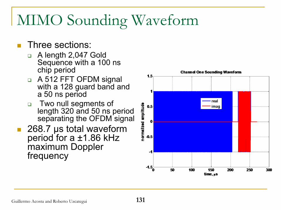
MIMO Sounding WaveformThree sections:
A length 2,047 Gold Sequence with a 100 ns chip periodA 512 FFT OFDM signal with a 128 guard band and a 50 ns periodTwo null segments of length 320 and 50 ns period separating the OFDM signal
268.7 μs total waveform period for a ±1.86 kHz maximum Doppler frequency
131Guillermo Acosta and Roberto Uzcategui
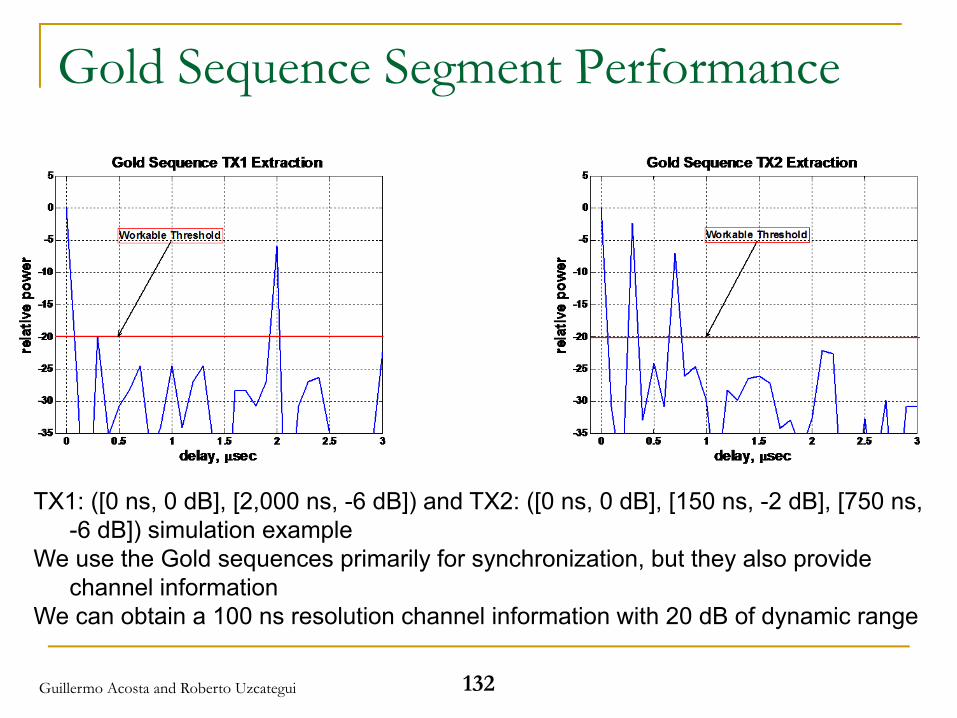
Gold Sequence Segment Performance
TX1: ([0 ns, 0 dB], [2,000 ns, -6 dB]) and TX2: ([0 ns, 0 dB], [150 ns, -2 dB], [750 ns, -6 dB]) simulation example
We use the Gold sequences primarily for synchronization, but they also provide channel information
We can obtain a 100 ns resolution channel information with 20 dB of dynamic range
132Guillermo Acosta and Roberto Uzcategui
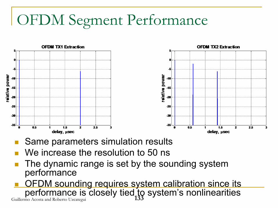
OFDM Segment Performance
Same parameters simulation resultsWe increase the resolution to 50 nsThe dynamic range is set by the sounding system performanceOFDM sounding requires system calibration since its performance is closely tied to system’s nonlinearities
133Guillermo Acosta and Roberto Uzcategui
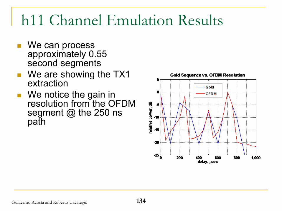
h11 Channel Emulation ResultsWe can process approximately 0.55 second segmentsWe are showing the TX1 extractionWe notice the gain in resolution from the OFDM segment @ the 250 ns path
134Guillermo Acosta and Roberto Uzcategui
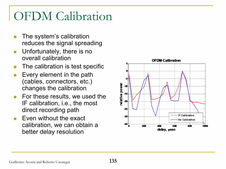
OFDM CalibrationThe system’s calibration reduces the signal spreadingUnfortunately, there is no overall calibrationThe calibration is test specificEvery element in the path (cables, connectors, etc.) changes the calibrationFor these results, we used the IF calibration, i.e., the most direct recording pathEven without the exact calibration, we can obtain a better delay resolution
135Guillermo Acosta and Roberto Uzcategui
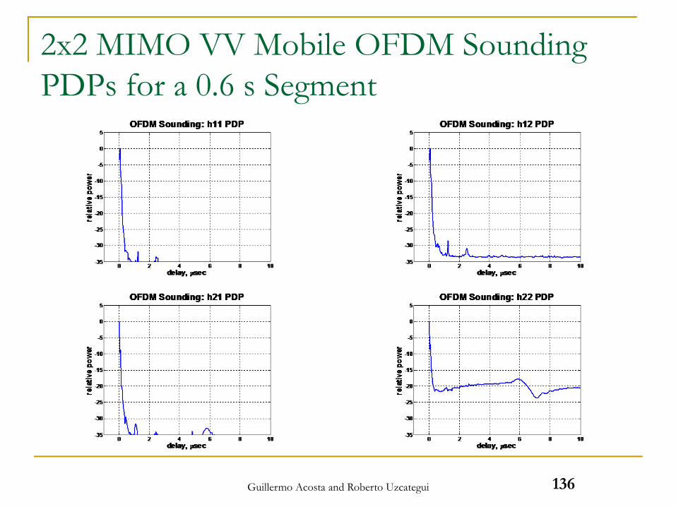
2x2 MIMO VV Mobile OFDM Sounding PDPs for a 0.6 s Segment
136Guillermo Acosta and Roberto Uzcategui
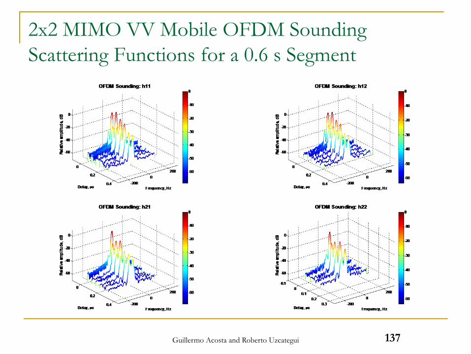
2x2 MIMO VV Mobile OFDM Sounding Scattering Functions for a 0.6 s Segment
137Guillermo Acosta and Roberto Uzcategui
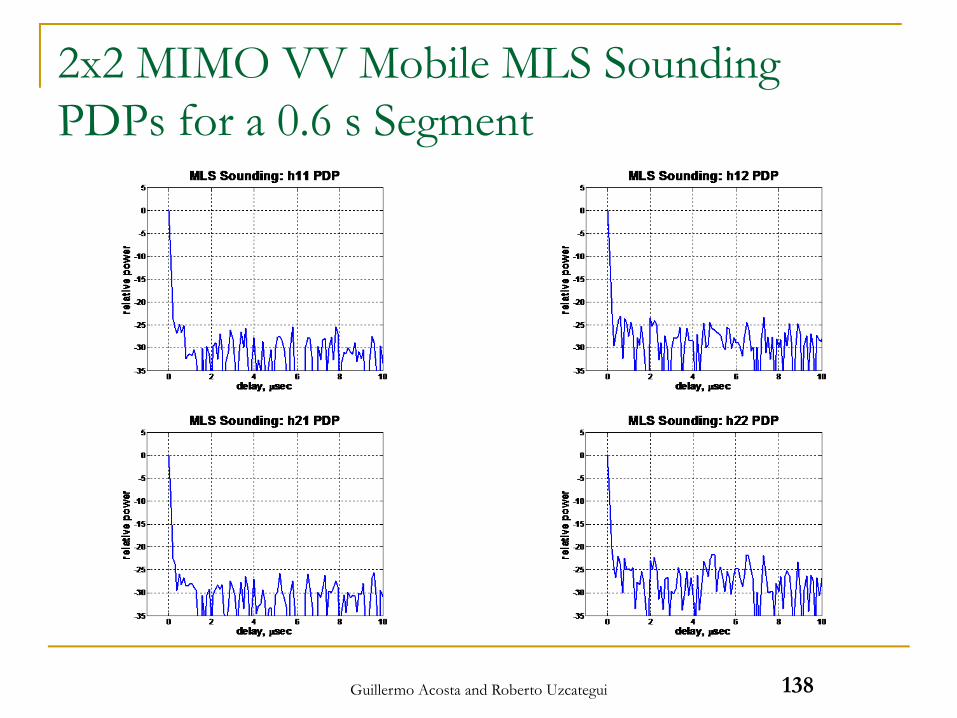
2x2 MIMO VV Mobile MLS Sounding PDPs for a 0.6 s Segment
138Guillermo Acosta and Roberto Uzcategui
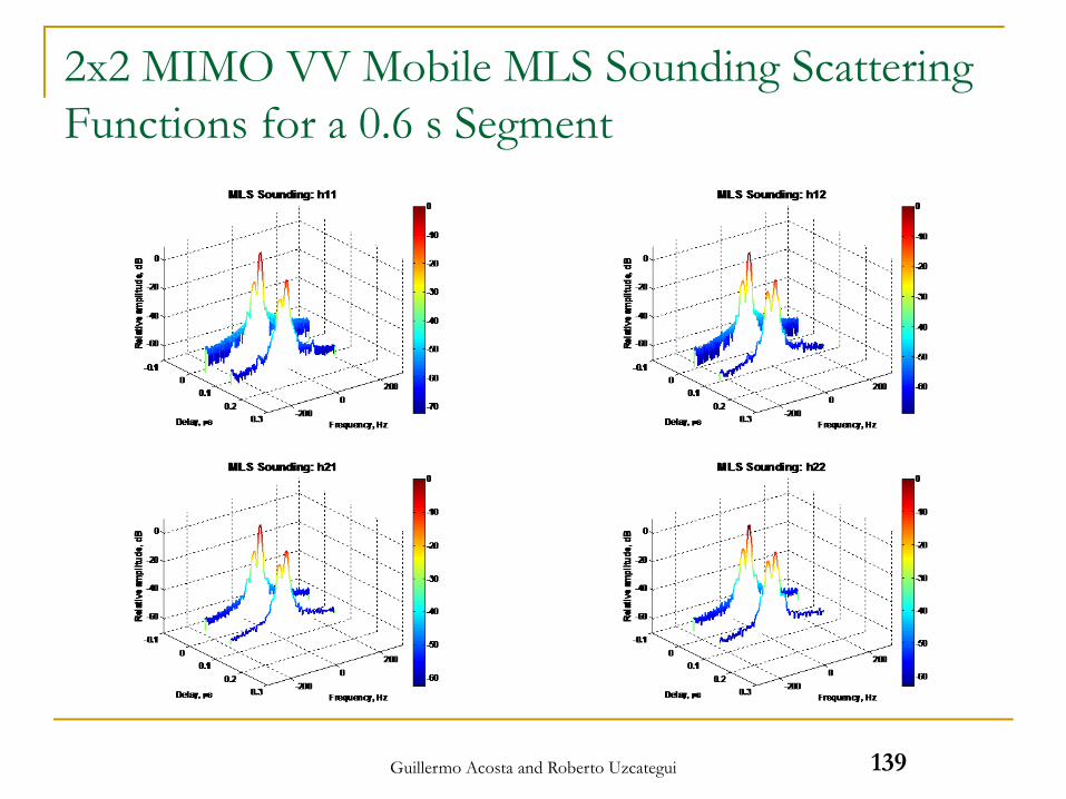
2x2 MIMO VV Mobile MLS Sounding Scattering Functions for a 0.6 s Segment
139Guillermo Acosta and Roberto Uzcategui
Thank you!