Water Resource Inventory and Assessment: Cape Romain

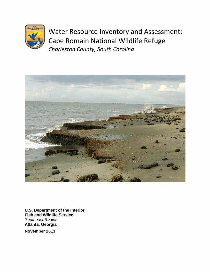
Water Resource Inventory and Assessment: Cape Romain National Wildlife Refuge Charleston County, South Carolina

U.S. Department of the Interior Fish and Wildlife Service Southeast Region Atlanta, Georgia

November 2013

ii

Water Resource Inventory and Assessment: Cape Romain National Wildlife Refuge Charleston County, South Carolina John Faustini U.S. Fish and Wildlife Service, Southeast Region 1875 Century Blvd., Suite 200 Atlanta, GA 30345 Theresa A. Thom U.S. Fish and Wildlife Service, Inventory and Monitoring Network Savannah Coastal Refuge Complex 694 Beech Hill Lane Hardeeville, SC 29927 Raye Nilius U.S. Fish and Wildlife Service South Carolina Refuges Complex 5801 Highway 17 North Awendaw, SC 29429 Kirsten J. Hunt and Rebecca E. Burns Atkins North America, Inc. 1616 East Millbrook Road, Suite 310 Raleigh, NC 27609 November 2013 U.S. Department of the Interior, U.S. Fish and Wildlife Service Please cite this publication as: Faustini, J., T.A. Thom, K.J. Hunt, R. Nilius, and R.E. Burns. 2013. Water Resource Inventory and Assessment: Cape Romain National Wildlife Refuge, Charleston County, South Carolina. U.S. Fish and Wildlife Service, Southeast Region. Atlanta, Georgia. November 2013, 84 p. COVER PHOTO: View to south along the coast of Cape Island, Cape Romain National Wildlife Refuge, South Carolina, 2009. Note the low vertical scarp formed by the cohesive sediments of the eroding tidal marsh platform exposed by the landward-retreating beach dune (out of the frame to the right). Photo credit: Steve Hillebrand/USFWS (retired). Used by permission.

iii

ACKNOWLEDGEMENTS: This work was completed in part through contract PO# F11PD00794 between the U.S. Fish and Wildlife Service and Atkins North America, Inc. Information for this report was compiled through coordination with multiple state and federal partners and non-governmental agencies, including the U.S. Fish and Wildlife Service (USFWS), South Carolina Department of Health and Environmental Control (SCDHEC), South Carolina Department of Natural Resources (SCDNR), and the U.S. Geological Survey (USGS). Significant input was provided by Cape Romain National Wildlife Refuge staff including Dan Ashworth and Sarah Dawsey. The authors thank Mark Cantrell (USFWS), Thomas Rainwater (USFWS), Bruce Campbell (USGS), Dave Chestnut (SCDHEC), Andy Miller (SCDHEC), and Zoe Hughes (Boston University) for thoughtful review comments on an earlier draft of this report and for generously sharing their time, expertise, and knowledge. The findings and conclusions in this report are those of the authors and do not necessarily represent the views of the U.S. Fish and Wildlife Service.

iv

Table of Contents

1 Executive Summary ............................................................................................................................. 1

1.1 Findings .......................................................................................................................................... 1

1.2 Key Water Resources Issues of Concern ........................................................................................ 2

1.3 Needs and Recommendations ....................................................................................................... 3

2 Introduction ........................................................................................................................................ 6

3 Facility Information ............................................................................................................................. 7

4 Natural Setting .................................................................................................................................. 11

4.1 Topography and Physiographic Setting ........................................................................................ 11

4.2 Climate ......................................................................................................................................... 11

4.2.1 Temperature and Precipitation ............................................................................................. 11

4.2.2 Extreme Weather Events ....................................................................................................... 14

4.3 Geology and Geomorphology ...................................................................................................... 15

4.3.1 Origin of the Modern Coastal Landscape .............................................................................. 15

4.3.2 Geomorphology and Coastal Processes ................................................................................ 16

4.4 Soils .............................................................................................................................................. 18

4.5 Hydrologic Setting ........................................................................................................................ 18

4.6 Historical Landscape Changes ...................................................................................................... 20

4.6.1 Hydrologic Alterations ........................................................................................................... 20

4.6.2 Development and Climate Change Impacts on Coastal Processes ........................................ 22

4.7 Climate Change ............................................................................................................................ 25

4.7.1 Climate Change Projections ................................................................................................... 25

4.7.2 Sea-level rise .......................................................................................................................... 27

4.7.3 SLAMM Modeling .................................................................................................................. 29

4.7.4 Storm Frequency and Intensity ............................................................................................. 33

5 Inventory Summary and Discussion .................................................................................................. 34

5.1 Water Resources .......................................................................................................................... 34

5.1.1 Rivers and Streams ................................................................................................................ 34

5.1.2 Canals and Drainage Ditches ................................................................................................. 34

5.1.3 Lakes and Ponds .................................................................................................................... 37

5.1.4 Wetlands ................................................................................................................................ 37

5.1.5 Groundwater ......................................................................................................................... 42

5.2 Infrastructure ............................................................................................................................... 43

v

5.2.1 Water Supply and Wastewater .............................................................................................. 43

5.2.2 Water Control Structures ...................................................................................................... 46

5.2.3 Ditches ................................................................................................................................... 46

5.2.4 Dikes and Levees.................................................................................................................... 46

5.3 Monitoring.................................................................................................................................... 50

5.3.1 Surface Water ........................................................................................................................ 54

5.3.2 Groundwater ......................................................................................................................... 62

5.3.3 Aquatic Habitat and Biota ...................................................................................................... 63

5.3.4 Other Relevant Monitoring ................................................................................................... 64

5.4 Water Quality Conditions ............................................................................................................. 64

5.4.1 State Water Quality Regulations ........................................................................................... 64

5.4.2 Impaired Waters and TMDLs ................................................................................................. 65

5.4.3 Other Surface Water Quality Information ............................................................................. 70

5.4.4 Groundwater Quality ............................................................................................................. 70

6 Water Law and Water Rights ............................................................................................................ 71

7 Assessment........................................................................................................................................ 72

7.1 Water Resource Issues of Concern .............................................................................................. 72

7.1.1 Urgent/Immediate Issues ...................................................................................................... 72

7.1.2 Longer-Term Issues ................................................................................................................ 74

7.2 Needs and Recommendations ..................................................................................................... 74

8 Literature Cited ................................................................................................................................. 77

vi

Appendices

Appendix A Cape Romain NWR Lease Agreement with the State of South Carolina

Appendix B Data Plots from U.S. Historical Climatology Network (USHCN) Stations Near Cape Romain NWR

Appendix C Pan Evaporation Records for the South Carolina Area

Appendix D GIS Analysis of Barrier Island Changes at Cape Romain NWR, 1875-2011

Appendix E Dike History (1938-2004) on Cape Romain NWR Based on Refuge Annual Narratives

Appendix F Preliminary Statement of Work: American Recovery and Reinvestment Act Projects Located at Cape Romain National Wildlife Refuge and Bears Bluff National Fish Hatchery

Appendix G Preliminary Scope of Work for Proposed Cross-Dike at Jacks Creek

Appendix H Water Quality Monitoring Data for Bulls Island, 2011-2012

Appendix I Historical Maps for Bulls Island and Vicinity, Cape Romain NWR

vii

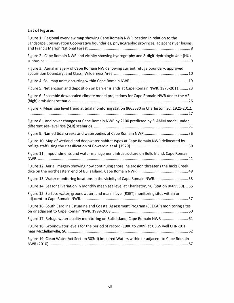
List of Figures

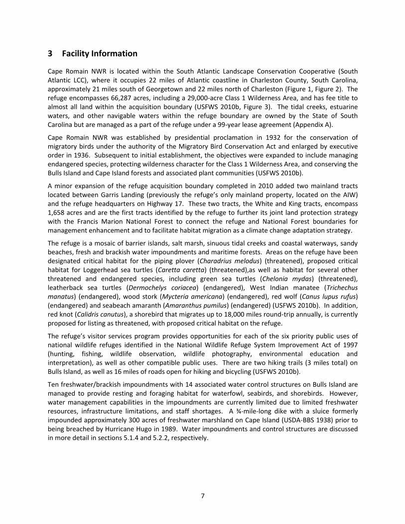
Figure 1. Regional overview map showing Cape Romain NWR location in relation to the Landscape Conservation Cooperative boundaries, physiographic provinces, adjacent river basins, and Francis Marion National Forest. ................................................................................................ 8

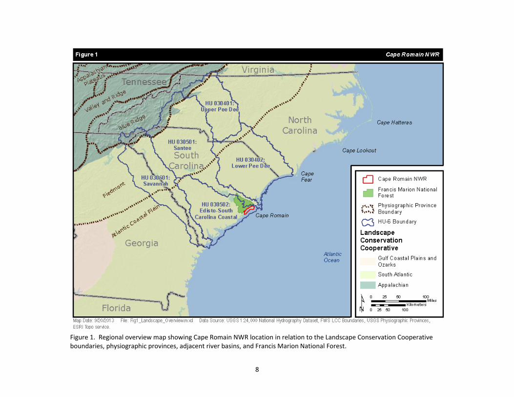
Figure 2. Cape Romain NWR and vicinity showing hydrography and 8-digit Hydrologic Unit (HU) subbasins. ......................................................................................................................................... 9

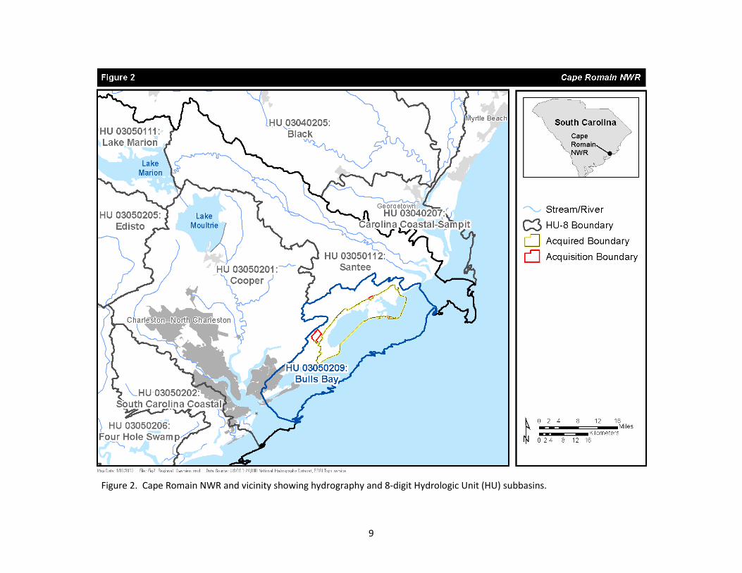
Figure 3. Aerial imagery of Cape Romain NWR showing current refuge boundary, approved acquisition boundary, and Class I Wilderness Area. ...................................................................... 10

Figure 4. Soil map units occurring within Cape Romain NWR. ...................................................... 19

Figure 5. Net erosion and deposition on barrier islands at Cape Romain NWR, 1875-2011......... 23

Figure 6. Ensemble downscaled climate model projections for Cape Romain NWR under the A2 (high) emissions scenario. .............................................................................................................. 26

Figure 7. Mean sea level trend at tidal monitoring station 8665530 in Charleston, SC, 1921-2012. ....................................................................................................................................................... 27

Figure 8. Land cover changes at Cape Romain NWR by 2100 predicted by SLAMM model under different sea-level rise (SLR) scenarios. ......................................................................................... 31

Figure 9. Named tidal creeks and waterbodies at Cape Romain NWR. ......................................... 36

Figure 10. Map of wetland and deepwater habitat types at Cape Romain NWR delineated by refuge staff using the classification of Cowardin et al. (1979). ..................................................... 39

Figure 11. Impoundments and water management infrastructure on Bulls Island, Cape Romain NWR. .............................................................................................................................................. 41

Figure 12. Aerial imagery showing how continuing shoreline erosion threatens the Jacks Creek dike on the northeastern end of Bulls Island, Cape Romain NWR. ............................................... 48

Figure 13. Water monitoring locations in the vicinity of Cape Romain NWR. ............................... 53

Figure 14. Seasonal variation in monthly mean sea level at Charleston, SC (Station 8665530). .. 55

Figure 15. Surface water, groundwater, and marsh level (RSET) monitoring sites within or adjacent to Cape Romain NWR. ..................................................................................................... 57

Figure 16. South Carolina Estuarine and Coastal Assessment Program (SCECAP) monitoring sites on or adjacent to Cape Romain NWR, 1999-2008. ........................................................................ 60

Figure 17. Refuge water quality monitoring on Bulls Island, Cape Romain NWR ......................... 61

Figure 18. Groundwater levels for the period of record (1980 to 2009) at USGS well CHN-101 near McClellanville, SC. .................................................................................................................. 62

Figure 19. Clean Water Act Section 303(d) Impaired Waters within or adjacent to Cape Romain NWR (2010). ................................................................................................................................... 67

viii

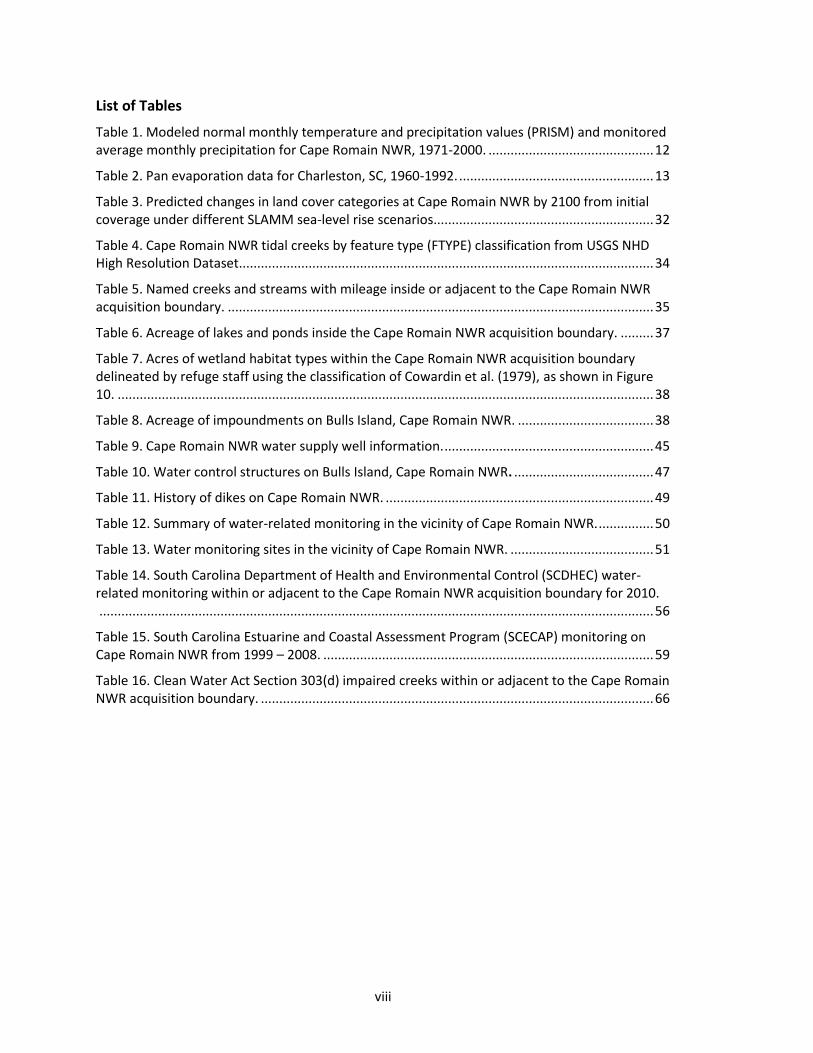
List of Tables

Table 1. Modeled normal monthly temperature and precipitation values (PRISM) and monitored average monthly precipitation for Cape Romain NWR, 1971-2000. ............................................. 12

Table 2. Pan evaporation data for Charleston, SC, 1960-1992. ..................................................... 13

Table 3. Predicted changes in land cover categories at Cape Romain NWR by 2100 from initial coverage under different SLAMM sea-level rise scenarios............................................................ 32

Table 4. Cape Romain NWR tidal creeks by feature type (FTYPE) classification from USGS NHD High Resolution Dataset................................................................................................................. 34

Table 5. Named creeks and streams with mileage inside or adjacent to the Cape Romain NWR acquisition boundary. .................................................................................................................... 35

Table 6. Acreage of lakes and ponds inside the Cape Romain NWR acquisition boundary. ......... 37

Table 7. Acres of wetland habitat types within the Cape Romain NWR acquisition boundary delineated by refuge staff using the classification of Cowardin et al. (1979), as shown in Figure 10. .................................................................................................................................................. 38

Table 8. Acreage of impoundments on Bulls Island, Cape Romain NWR. ..................................... 38

Table 9. Cape Romain NWR water supply well information. ......................................................... 45

Table 10. Water control structures on Bulls Island, Cape Romain NWR. ...................................... 47

Table 11. History of dikes on Cape Romain NWR. ......................................................................... 49

Table 12. Summary of water-related monitoring in the vicinity of Cape Romain NWR. ............... 50

Table 13. Water monitoring sites in the vicinity of Cape Romain NWR. ....................................... 51

Table 14. South Carolina Department of Health and Environmental Control (SCDHEC) water-related monitoring within or adjacent to the Cape Romain NWR acquisition boundary for 2010. ....................................................................................................................................................... 56

Table 15. South Carolina Estuarine and Coastal Assessment Program (SCECAP) monitoring on Cape Romain NWR from 1999 – 2008. .......................................................................................... 59

Table 16. Clean Water Act Section 303(d) impaired creeks within or adjacent to the Cape Romain NWR acquisition boundary. ........................................................................................................... 66

1

1 Executive Summary

This Water Resource Inventory and Assessment (WRIA) Summary Report for Cape Romain National Wildlife Refuge (Cape Romain NWR or the refuge) summarizes available information relevant to refuge water resources, provides an assessment of refuge water resource needs and issues of concern, and makes recommendations regarding potential actions that might be considered to address the identified water resources needs and concerns. Major topics addressed in this report include the natural setting of the refuge (topography, climate, geology, soils, hydrology), impacts of development and climate change, significant water resources and associated infrastructure within the refuge, past and current water monitoring activities on and near the refuge, water quality information, and state water use regulatory framework. Information was compiled from publicly available reports, databases, and geospatial datasets from federal, state, and local agencies; published research reports; websites maintained by government agencies, academic institutions, and non-governmental organizations; and from files and Geographical Information Systems (GIS) data layers maintained by the refuge. The following three subsections summarize key findings of the WRIA, major water resource issues of concern identified, and recommendations to address priority water resource threats and needs.

1.1 Findings

Cape Romain NWR in Charleston County, South Carolina protects approximately 66,287 acres, including a 29,000-acre Class 1 Wilderness Area. Coastal habitat within the refuge includes barrier islands, tidal salt marshes, managed wetland impoundments, white sand beaches, and drier upland areas dominated by a maritime forest of loblolly pine (Pinus taeda) and associated hardwood species. Aside from one small parcel, the refuge is separated from the mainland by the Atlantic Intracoastal Waterway (AIW), a 90-foot wide shipping canal dredged to a depth of 12 feet (ft).

The landscape in which Cape Romain NWR is situated has been shaped by numerous climate-driven sea level changes associated with glacial-interglacial cycles over the past 3-4 million years. Locally, sea level has been rising for the last 18,000 years at a gradually declining rate, but the rate of sea-level rise has accelerated in the past 100 years.

Major factors shaping this dynamic coastal system include sea-level rise, hurricanes and tropical storms, extra-tropical cyclones, strong winds, and tidal movement of water, which continually redistribute sediments and reshape barrier islands, tidal marsh, and other coastal landforms.

There is evidence that the frequency and intensity of Atlantic tropical cyclones has increased significantly since about 1970, and that this trend will likely continue as the climate warms.

Significant man-made hydrologic alterations to the landscape surrounding the refuge include construction of the AIW (begun in the early 1900s and completed by 1940) and damming and diversion of the Santee River in 1941. The latter greatly reduced sediment delivery to the Santee delta, and both projects affect salinity in tidal estuaries, particularly in the northern part of the refuge.

Refuge staff classified habitat types within the refuge acquisition boundary using the Cowardin Classification System methods. The results revealed that approximately 48.39% of the refuge is estuarine and marine wetlands, 44.70% is estuarine and marine deepwater aquatic sites, 4.94% is upland or unclassified habitats, 1.73% is freshwater forested/shrub-wetlands, and 0.24% is freshwater emergent wetlands. These values differ slightly from those derived from National Wetlands Inventory (NWI) data, with the most significant differences occurring on Bulls Island, where NWI does not accurately represent managed wetland impoundments, and the other barrier

2

islands, where NWI data do not reflect recent changes in the shape and extent of these dynamic features.

Cape Romain NWR contains approximately 470 miles of tidal streams and creeks within or adjacent to the acquisition boundary; there are no non-tidal freshwater streams. The refuge also contains 10 impoundments totaling 756.1 acres on Bulls Island that are managed to provide resting and foraging habitat for waterfowl, seabirds, and shorebirds.

As of 2010, 17 creeks or creek segments located within or adjacent to the refuge acquisition boundary were listed as impaired for aquatic life or recreation by the South Carolina Department of Health and Environmental Control. Causes of impairment include turbidity, total ammonia, and copper levels that are out of compliance, resulting in impaired ability of the waterbody to support aquatic life, as well as fecal coliform bacteria levels that exceed the safe limit for primary contact recreation or shellfish harvest.

Tidal creeks, estuarine waters, and other navigable waters within the refuge boundary are owned by the State of South Carolina but are managed as part of the refuge by the U.S. Fish and Wildlife Service (USFWS) under a 99-year lease agreement. The lease agreement grants management authority over the water and water bottoms within the refuge boundary to the USFWS, with the exception of fin fish, shellfish, and other saltwater species take, which is regulated by the State.

Cape Romain NWR is located within the state-designated Trident Capacity Use Area, within which any person or entity withdrawing over 3 million gallons in any month is required to obtain a permit from and report annual water use to SCDHEC. However, South Carolina law specifically exempts from regulation any groundwater or surface water withdrawals for the purpose of wildlife habitat management.

1.2 Key Water Resources Issues of Concern

Although not strictly a water resource issue, the overriding threat to the refuge’s ability to fulfill its mission into the future—indeed, to continue to exist at all—is the issue of accelerated sea-level rise (SLR) and associated climate change impacts caused by anthropogenic greenhouse gas emissions. Long-term sea level trends suggest the local sea level is rising about 3.10 millimeters per year (mm/yr), based on mean monthly sea level data from Charleston Harbor for 1921 to 2012, or roughly double the global average rate of 1-2 mm/yr over the 20th century (Church et al. 2001). (Local SLR rates at any given location can be higher or lower than the global SLR rate due to local effects such as glacial isostatic adjustment, tectonic uplift, or subsidence.) While there is considerable uncertainty about future rates of sea-level rise, recent modeling studies updated to incorporate ice sheet melting suggest that eustatic (global) sea level could rise by up to 2 m by the end of this century, equivalent to an average rate of about 22 mm/yr (Burkett and Davidson 2012). For low-lying coastal regions like the South Carolina coast, erosion, inundation and shoreline retreat are expected to be the dominant response to sea-level rise and storms over this century and beyond. For some barrier islands and wetlands, higher sea-level rise scenarios will cause significant and irreversible changes including rapid landward migration and segmentation of some barrier islands as well as disintegration and drowning of tidal wetlands (Williams and Gutierrez 2009).

Specific issues of urgent concern at Cape Romain NWR include the following:

1. There is an imminent threat of breaching of the perimeter dike on the seaward side of the Jacks Creek impoundment on Bulls Island due to ongoing rapid shoreline erosion. Breaching of the dike would convert Jacks Creek from an actively managed brackish water wetland to passively managed intertidal habitat. This would result in the immediate loss of nearly two-thirds of the refuge’s managed wetland acres and would threaten the remaining impoundments (and the freshwater

3

supply upon which all the island’s wildlife depend) by exposing the lower internal dikes to potential overwash by seawater during even moderate storms.

2. Rapid erosion of barrier islands due to sea-level rise and possible intensification of storm magnitude and/or frequency is reducing and threatens to eliminate nesting, foraging, and resting habitat for Federal Trust species including threatened loggerhead sea turtles (Caretta caretta), threatened piping plover (Charadrius melodus), red knot (Calidris canutus) (currently proposed for listing with proposed critical habitat on the refuge), other species of shorebirds whose populations are in significant decline, seabirds, and habitat for endangered seabeach amaranth (Amaranthus pumilus), particularly on Cape and Lighthouse Islands. Erosion of the barrier islands has likely been exacerbated by disruption of natural sediment transport processes by coastal and riverine engineering projects including dams on the Santee and Cooper rivers, the AIW, jetties at the entrance to Winyah Bay, and dredging to maintain navigations channels in the Santee River estuary and Winyah Bay.

3. The salt marsh in the 29,000-acre Class I Wilderness Area is currently undergoing fragmentation, inundation, and salinity changes associated with relative sea-level rise. The marsh is vital nursery habitat for juvenile fish, crabs, and shrimp that take refuge among the vegetation for protection from predators. These species are the foundation of the food chain upon which coastal species are dependent.

4. The supply of freshwater for habitat management in the Bulls Island impoundments is unreliable and often insufficient during dry years due to reliance on rainfall. Groundwater wells drilled on Bulls Island have provided only limited quantities of generally poor-quality water.

5. The ability to manage impoundments on Bulls Island to achieve desired habitat conditions is also currently limited due to reliance on gravity flow to move water among impoundments, infrastructure limitations involving water conveyance channels, and the absence of staff to manage the system.

Somewhat longer-term issues of concern include the following:

1. Armoring and continuing development of adjacent and nearby properties limit the capacity for habitat shifts to occur in response to sea-level rise and threaten to constrain future management options. Development of mainland coastal properties between the refuge and Francis Marion National Forest could prevent acquisition and preservation of migration corridors for coastal-dependent species and their habitats.

2. Urban development, deforestation, and failing septic systems have and will continue to have an adverse effect on water quality at the refuge. Impacts include elevated turbidity and nutrients, human pathogens, organic contaminants, and altered salinity.

1.3 Needs and Recommendations

1. To mitigate for the anticipated breaching of the seaward dike enclosing the Jacks Creek impoundment as a result of continued erosion, construction of a cross-dike through Jacks Creek impoundment has been proposed at an estimated cost of $3 million (USFWS 2010b, Appendix F). The cross-dike would preserve approximately half of the existing impoundment and protect interior dikes and impoundments (and recently replaced water control structures) from direct exposure to tidal fluctuations and wave action. It is anticipated that this action would allow the refuge to continue to manage the remaining impoundments for migratory bird habitat for at least 20 years. If a decision is made to proceed with the cross-dike, it is critically important that it be completed before the existing seaward portion of Jacks Creek dike is breached, which is expected to occur sometime within the next few years given current shoreline erosion rates.

4

2. To provide a reliable freshwater supply for habitat management in the impoundments on Bulls Island, a deep (approximately 1,800 ft) groundwater supply well could be drilled to draw water from the Charleston aquifer. Such a well would almost certainly be capable of providing an adequate supply of water of adequate quality to meet refuge management needs on Bulls Island.

3. An updated water management plan should be prepared by a qualified contractor or partner organization with the necessary hydrologic and engineering expertise. The plan should include a field-based assessment of water management capabilities, including a survey of elevations and grades of water control structures (WCS) and conveyance channels, and should make specific recommendations for improvements or maintenance (e.g., clearing or re-grading of ditches, acquisition of portable high-volume low-head pumps, etc.) needed to provide sufficient water management capabilities to maintain desired habitat conditions in the managed wetland impoundments on Bulls Island. The plan should consider potential impacts of sea-level rise on the water management system as a whole to ensure that recommended improvements do not increase the vulnerability of any of the impoundments to continued sea-level rise.

4. A water monitoring plan for the refuge should be developed and implemented, either as part of the Inventory and Monitoring Plan for the refuge, or as a stand-alone document. Water monitoring efforts are tied to baseline information needs in the adaptive management framework, targeting ecological integrity while meeting refuge level, regional, and national Water Resources Inventory and Monitoring Goals and Objectives (USFWS 2010a, USFWS 2013). Specific tasks should include the following elements:

Monitor water levels and basic water quality parameters (temperature, pH, salinity, and dissolved oxygen [DO]) in the Bulls Island impoundments. Depending upon available resources, it would also be helpful to install some shallow wells in the vicinity of the impoundments to monitor seasonal fluctuations and long-term changes (e.g., in response to sea-level rise) in groundwater levels and groundwater quality (particularly salinity) and to assess potential impacts on water levels and water quality in the impoundments.

Water quality monitoring (temperature, pH, salinity, turbidity, DO, and nutrients) in tidal channels at selected locations—ideally at several fixed locations and several randomly selected temporary (rotating) locations.

Ideally, supplement water quality monitoring at fixed points with seasonal synoptic surveys to better characterize spatial water quality patterns (and seasonal variation in those patterns).

Continuous tidal water level monitoring at one or more fixed locations (e.g., Garris Landing).

5. Implementation of the plans described in Recommendations 3 and 4 above (i.e., managing water levels and habitat conditions in the Bulls Island impoundments and conducting water monitoring) would require additional staff resources. It is estimated that these tasks would require approximately 0.25-0.5 full-time equivalents (FTE) by a hydrologic technician or similarly qualified staff person to fully implement.

6. Obtaining high-quality LiDAR data covering the entire refuge and adjacent inland areas is a high-priority data need for refuge planning purposes. If existing data prove to be inadequate (including full coverage for northern Charleston County acquired by the South Carolina LiDAR Consortium in 2009 but not yet released due to data processing issues), the refuge should explore opportunities to partner with other stakeholders (e.g., local and state government agencies, non-governmental organizations [NGOs], Frances Marion National Forest, etc.) to obtain suitable LiDAR data.

5

7. Develop and implement a plan to monitor sea-level rise impacts on coastal erosion on barrier islands and on fragmentation and conversion of tidal marsh. Elements of the plan could include the following:

Once LiDAR data have been obtained, run a new SLAMM analysis using LiDAR-derived elevation data and customized land cover data (e.g., modified NWI land cover with ground-truthed cover classes). The analysis area should extend several miles inland from the existing refuge boundary and ideally should include the Santee River delta.

Continue monitoring barrier island and shoreline erosion with updated aerial imagery and ground-based measurements. Expand geospatial analysis beyond the four primary barrier islands to all land and marsh on the refuge. Develop a baseline analysis and monitor regularly as new imagery becomes available to track accretion, erosion, and tidal creek expansion.

Explore funding and/or partnership opportunities to install additional sediment elevation table (SET) stations to monitor marsh accretion, subsidence, and surface elevation changes closer to the mainland in high marsh.

8. In partnership with the U.S. Forest Service, state agencies, and NGOs, develop a long-term, landscape-scale strategy for responding to sea-level rise. Connecting protected areas that extend from refuge estuaries to the Francis Marion National Forest will create corridors that will allow for species and habitat migration in the future. Because continued rapid development on the mainland adjacent to the refuge could severely limit future management options involving new land acquisition or easements within the next decade, it is essential to develop and begin implementing such an adaptation strategy soon as possible.

9. Build upon existing partnerships and explore new partnership opportunities with other federal and state agencies, NGOs, and academic institutions to carry out relevant research for habitat and species management and baseline data needs in light of continued urban development, sea-level rise, and climate change impacts. Examples of identified research needs include the following:

Examine the effects of groundwater inundation and saltwater intrusion due to sea-level rise on sea turtle nests in the refuge.

Replicate the Bulls Island vegetation study by Mixon (2002) to show changes in habitat composition from saltwater intrusion.

6

2 Introduction

This WRIA Summary Report for Cape Romain NWR summarizes available information relevant to refuge water resources, provides an assessment of refuge water resource needs and issues of concern, and makes recommendations regarding potential actions that might be considered to address the identified water resources needs and concerns. The information compiled in preparing this report will ultimately be housed in an online WRIA database currently under development by the Natural Resources Program Center (NRPC), which is expected to be operational by mid-2014. Together, the WRIA Summary Report and the accompanying information in the online WRIA database are intended to be a reference to guide ongoing water resource management and strategy development. This WRIA Summary Report was developed in conjunction with the South Carolina Lowcountry Refuges Complex Project Leader, the refuge manager, refuge biologists, Inventory & Monitoring (I&M) zone biologists, and refuge staff. The document incorporates hydrologic information compiled between February 2012 and July 2013.

Together, the national interactive online WRIA database and the summary reports are designed to provide a reconnaissance-level inventory and assessment of water resources on and adjacent to National Wildlife Refuges and National Fish Hatcheries nationwide. Achieving a greater understanding of existing refuge water resources will help identify potential concerns or threats to those resources and will provide a basis for wildlife habitat management and operational recommendations to refuge managers, wildlife biologists, field staff, Regional Office personnel, and Department of Interior managers. A national team composed of USFWS Water Resource staff, Environmental Contaminants Biologists, and other USFWS employees developed the standardized content of the national interactive online WRIA database and summary reports.

The long term goal of the National Wildlife Refuge System (NWRS) WRIA effort is to provide up-to-date, accurate data on NWRS water quantity and quality in order to acquire, manage, and protect adequate supplies of clean and freshwater. An accurate water resources inventory is essential to prioritize issues and tasks, and to take prescriptive actions that are consistent with the established purposes of the refuge. Reconnaissance-level water resource assessments evaluate water rights, water quantity, known water quality issues, water management, potential water acquisitions, threats to water supplies, and other water resource issues for each field station.

WRIAs are recognized as an important part of the NWRS I&M initiative and are outlined in the I&M Operational Blueprint as Task 2a (USFWS 2010a). Hydrologic and water resource information compiled during the WRIA process can facilitate the development of other key documents for each refuge including Hydrogeomorphic Assessments (HGMs), Comprehensive Conservation Plans (CCPs), and Habitat Management Plans (HMPs).

A CCP for the refuge was completed in October 2010 and a HMP is scheduled to be completed by the end of 2013. Completion of a WRIA for Cape Romain NWR was prioritized largely to facilitate ongoing planning efforts, including the HMP and a HGM that was initiated concurrently with this WRIA. Key water resource issues of concern identified by the CCP include shoreline erosion due to the effects of sea-level rise and reduced sediment supply from the Santee River following construction of dams and canals in the 1940s, the desire to restore and maintain water management capabilities on Bulls Island, and water quality concerns including episodically high fecal coliform bacteria levels and inadequate water quality information.

7

3 Facility Information

Cape Romain NWR is located within the South Atlantic Landscape Conservation Cooperative (South Atlantic LCC), where it occupies 22 miles of Atlantic coastline in Charleston County, South Carolina, approximately 21 miles south of Georgetown and 22 miles north of Charleston (Figure 1, Figure 2). The refuge encompasses 66,287 acres, including a 29,000-acre Class 1 Wilderness Area, and has fee title to almost all land within the acquisition boundary (USFWS 2010b, Figure 3). The tidal creeks, estuarine waters, and other navigable waters within the refuge boundary are owned by the State of South Carolina but are managed as a part of the refuge under a 99-year lease agreement (Appendix A).

Cape Romain NWR was established by presidential proclamation in 1932 for the conservation of migratory birds under the authority of the Migratory Bird Conservation Act and enlarged by executive order in 1936. Subsequent to initial establishment, the objectives were expanded to include managing endangered species, protecting wilderness character for the Class 1 Wilderness Area, and conserving the Bulls Island and Cape Island forests and associated plant communities (USFWS 2010b).

A minor expansion of the refuge acquisition boundary completed in 2010 added two mainland tracts located between Garris Landing (previously the refuge’s only mainland property, located on the AIW) and the refuge headquarters on Highway 17. These two tracts, the White and King tracts, encompass 1,658 acres and are the first tracts identified by the refuge to further its joint land protection strategy with the Francis Marion National Forest to connect the refuge and National Forest boundaries for management enhancement and to facilitate habitat migration as a climate change adaptation strategy.

The refuge is a mosaic of barrier islands, salt marsh, sinuous tidal creeks and coastal waterways, sandy beaches, fresh and brackish water impoundments and maritime forests. Areas on the refuge have been designated critical habitat for the piping plover (Charadrius melodus) (threatened), proposed critical habitat for Loggerhead sea turtles (Caretta caretta) (threatened),as well as habitat for several other threatened and endangered species, including green sea turtles (Chelonia mydas) (threatened), leatherback sea turtles (Dermochelys coriacea) (endangered), West Indian manatee (Trichechus manatus) (endangered), wood stork (Mycteria americana) (endangered), red wolf (Canus lupus rufus) (endangered) and seabeach amaranth (Amaranthus pumilus) (endangered) (USFWS 2010b). In addition, red knot (Calidris canutus), a shorebird that migrates up to 18,000 miles round-trip annually, is currently proposed for listing as threatened, with proposed critical habitat on the refuge.

The refuge’s visitor services program provides opportunities for each of the six priority public uses of national wildlife refuges identified in the National Wildlife Refuge System Improvement Act of 1997 (hunting, fishing, wildlife observation, wildlife photography, environmental education and interpretation), as well as other compatible public uses. There are two hiking trails (3 miles total) on Bulls Island, as well as 16 miles of roads open for hiking and bicycling (USFWS 2010b).

Ten freshwater/brackish impoundments with 14 associated water control structures on Bulls Island are managed to provide resting and foraging habitat for waterfowl, seabirds, and shorebirds. However, water management capabilities in the impoundments are currently limited due to limited freshwater resources, infrastructure limitations, and staff shortages. A ¾-mile-long dike with a sluice formerly impounded approximately 300 acres of freshwater marshland on Cape Island (USDA-BBS 1938) prior to being breached by Hurricane Hugo in 1989. Water impoundments and control structures are discussed in more detail in sections 5.1.4 and 5.2.2, respectively.

8

Figure 1. Regional overview map showing Cape Romain NWR location in relation to the Landscape Conservation Cooperative boundaries, physiographic provinces, adjacent river basins, and Francis Marion National Forest.

9

Figure 2. Cape Romain NWR and vicinity showing hydrography and 8-digit Hydrologic Unit (HU) subbasins.

10

Figure 3. Aerial imagery of Cape Romain NWR showing current refuge boundary, approved acquisition boundary, and Class I Wilderness Area.

11

4 Natural Setting

4.1 Topography and Physiographic Setting

Cape Romain NWR is situated on the southeastern (outer) margin of the Atlantic Coastal Plain (ACP) along the central South Carolina coast between the Santee River estuary to the north and Charleston Harbor to the south (Figure 1 and Figure 2). The outer ACP ranges in elevation from 0 to 50 feet (0 to 15 m) above the National Geodetic Vertical Datum of 1929 (NGVD 29) and is characterized by gently rolling to flat topography that generally slopes southeastward toward the Atlantic Ocean (Campbell and Coes 2010). Elevations on the refuge range from 0 to 21 feet (0 to 6 m) NGVD 29. The refuge, which is separated from the mainland by the AIW, is primarily composed of barrier islands and salt marshes. The barrier islands are low in elevation with dunes and beaches on the ocean side and a mix of forest and wetlands (depending on elevation) on the interior side (USFWS 2010b).

4.2 Climate

4.2.1 Temperature and Precipitation

Climatic information presented in this WRIA comes from two sources (in addition to refuge-generated data): the U.S. Historical Climatology Network (USHCN) of monitoring sites maintained by the National Weather Service (Menne et al. undated) and the PRISM (Parameter-elevation Regressions on Independent Slopes Model) climate mapping service, which is the U.S. Department of Agriculture’s (USDA) official source of climatological data (PRISM 2010). The PRISM data (Table 1) represent 1971-2000 climatological normals, while the period of record for the USHCN data (Appendix B: Figures B1-B4) is 1895-2010. The closest USHCN stations are located in Charleston and Georgetown, SC.

The climate of the refuge is characterized by warm, humid summers and relatively mild, temperate winters. Mean monthly temperatures in the vicinity of the refuge range from approximately 51 °F (10.6 °C) in January to 82 °F (27.8 °C) in July and August at Charleston, with temperatures at Georgetown averaging about 4 to 5 °F (2.5 °C) cooler. Mean monthly temperatures exhibit the greatest year-to-year variability in the winter and early spring (December through March) and the least variability in mid-summer (July and August) (Appendix B: Figure B1). However, the monthly temperature range is a relatively uniform 17-21 °F throughout the year (Table 1). The mean daily temperature range is about twice as great at Charleston (22 °F) as at Georgetown (11 °F). No trends in mean annual daily minimum, mean, or maximum temperatures are apparent over the period of record at either Charleston or Georgetown (Appendix B: Figure B2).

Mean monthly precipitation (from PRISM dataset) varies by slightly more than a factor of two over the course of the year, with an average of 3.0 to 4.4 inches (in) (7.5 to 11.1 centimeters [cm]) falling in October through May and 5.8 to 6.7 in (14.7 to 17.0 cm) in June through September, with a mean annual total of 53.2 in (135.2 cm; Table 1). The wettest months (June-September) also have the greatest year-to-year variability in precipitation (Appendix B: Figure B3). Precipitation data collected by refuge staff at Bulls Island for the same period (1971-2000, but with missing data for 1973-75 and 1989) show very nearly the same total precipitation and generally the same seasonal pattern as the PRISM data, although the refuge measurements show approximately 10-20% less precipitation in May through July and December and 8-24% more precipitation in August through November (Table 1). Total precipitation shows a high degree of year-to-year variability as well as roughly decadal-scale oscillations at both the Charleston and Georgetown USHCN stations, although the oscillations are not always synchronous at the two stations (Appendix B: Figure B4). No long-term trend in precipitation is apparent at either location.

12

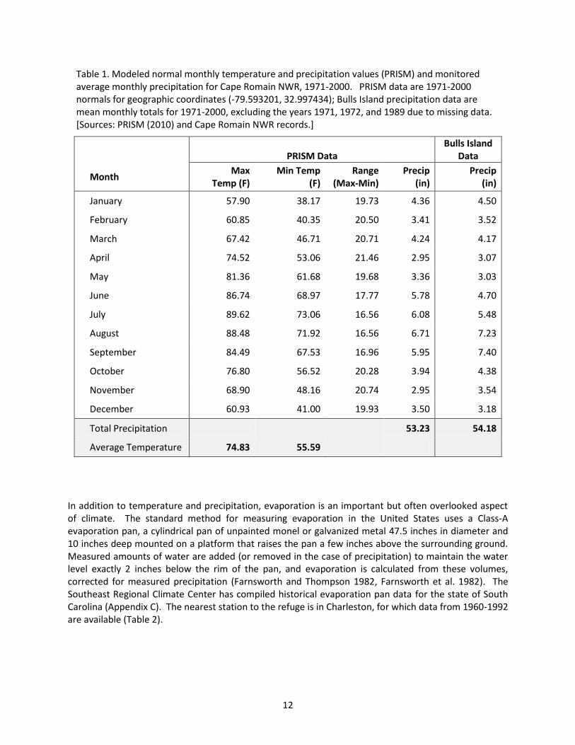
Table 1. Modeled normal monthly temperature and precipitation values (PRISM) and monitored average monthly precipitation for Cape Romain NWR, 1971-2000. PRISM data are 1971-2000 normals for geographic coordinates (-79.593201, 32.997434); Bulls Island precipitation data are mean monthly totals for 1971-2000, excluding the years 1971, 1972, and 1989 due to missing data. [Sources: PRISM (2010) and Cape Romain NWR records.]

PRISM Data

Bulls Island Data

Month Max

Temp (F) Min Temp

(F) Range

(Max-Min) Precip

(in) Precip

(in)

January 57.90 38.17 19.73 4.36 4.50

February 60.85 40.35 20.50 3.41 3.52

March 67.42 46.71 20.71 4.24 4.17

April 74.52 53.06 21.46 2.95 3.07

May 81.36 61.68 19.68 3.36 3.03

June 86.74 68.97 17.77 5.78 4.70

July 89.62 73.06 16.56 6.08 5.48

August 88.48 71.92 16.56 6.71 7.23

September 84.49 67.53 16.96 5.95 7.40

October 76.80 56.52 20.28 3.94 4.38

November 68.90 48.16 20.74 2.95 3.54

December 60.93 41.00 19.93 3.50 3.18

Total Precipitation

53.23 54.18

Average Temperature 74.83 55.59

In addition to temperature and precipitation, evaporation is an important but often overlooked aspect of climate. The standard method for measuring evaporation in the United States uses a Class-A evaporation pan, a cylindrical pan of unpainted monel or galvanized metal 47.5 inches in diameter and 10 inches deep mounted on a platform that raises the pan a few inches above the surrounding ground. Measured amounts of water are added (or removed in the case of precipitation) to maintain the water level exactly 2 inches below the rim of the pan, and evaporation is calculated from these volumes, corrected for measured precipitation (Farnsworth and Thompson 1982, Farnsworth et al. 1982). The Southeast Regional Climate Center has compiled historical evaporation pan data for the state of South Carolina (Appendix C). The nearest station to the refuge is in Charleston, for which data from 1960-1992 are available (Table 2).

13

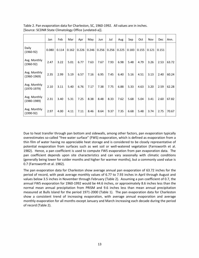
Table 2. Pan evaporation data for Charleston, SC, 1960-1992. All values are in inches. [Source: SCDNR State Climatology Office (undated-a)].

Jan Feb Mar Apr May Jun Jul Aug Sep Oct Nov Dec Ann.

Daily (1960-92)

0.080 0.114 0.162 0.226 0.246 0.256 0.256 0.225 0.183 0.155 0.121 0.151

Avg. Monthly (1960-92)

2.47 3.22 5.01 6.77 7.63 7.67 7.93 6.98 5.48 4.79 3.26 2.53 63.72


2.35 2.99 5.19 6.57 7.16 6.95 7.45 6.40 5.16 4.51 3.13 2.40 60.24


2.10 3.11 5.40 6.76 7.17 7.38 7.75 6.88 5.33 4.63 3.20 2.59 62.28


2.31 3.40 5.31 7.25 8.38 8.48 8.33 7.62 5.68 5.04 3.41 2.60 67.82


2.97 4.00 4.11 7.11 8.46 8.64 9.37 7.35 6.68 5.48 3.74 2.75 70.67

Due to heat transfer through pan bottom and sidewalls, among other factors, pan evaporation typically overestimates so-called “free water surface” (FWS) evaporation, which is defined as evaporation from a thin film of water having no appreciable heat storage and is considered to be closely representative of potential evaporation from surfaces such as wet soil or well-watered vegetation (Farnsworth et al. 1982). Hence, a pan coefficient is used to compute FWS evaporation from pan evaporation data. The pan coefficient depends upon site characteristics and can vary seasonally with climatic conditions (generally being lower for colder months and higher for warmer months), but a commonly used value is 0.7 (Farnsworth et al. 1982).

The pan evaporation data for Charleston show average annual pan evaporation of 63.72 inches for the period of record, with peak average monthly values of 6.77 to 7.93 inches in April through August and values below 3.5 inches in November through February (Table 2). Assuming a pan coefficient of 0.7, the annual FWS evaporation for 1960-1992 would be 44.6 inches, or approximately 8.6 inches less than the normal mean annual precipitation from PRISM and 9.6 inches less than mean annual precipitation measured at Bulls Island for the period 1971-2000 (Table 1). The pan evaporation data for Charleston show a consistent trend of increasing evaporation, with average annual evaporation and average monthly evaporation for all months except January and March increasing each decade during the period of record (Table 2).

14

4.2.2 Extreme Weather Events

An important influence on the climate of coastal South Carolina is the Bermuda High, a semi-permanent, subtropical area of high pressure in the North Atlantic Ocean that migrates east and west with varying central pressure. During the summer and fall it migrates westward and is typically centered in the western North Atlantic near Bermuda. In the winter and early spring it moves eastward to the vicinity of the Azores in the eastern North Atlantic and is known as the Azores High. The strength and position of the Bermuda High strongly influences the occurrence of drought in coastal South Carolina and also influences the course of tropical cyclones and hurricanes (SCDNR State Climatology Office undated-b, Trewartha 1981).

South Carolina has high interannual and seasonal variability of precipitation (Appendix B: figures B3 and B4), with the main cause of this variability being variation in the strength and placement of the Bermuda High. Periods of dry weather have occurred in each decade since 1818. The most damaging droughts in recent history occurred in 1954, 1986 and 1998-2002, with less severe droughts reported in 1988, 1990, 1993, and 1995 (SCDNR State Climatology Office undated-b).

Severe weather events in South Carolina include thunderstorms, tornadoes, tropical cyclones, and extra-tropical cyclones. Thunderstorms are most common in the summer months, but the more violent storms generally accompany squall lines and active cold fronts in late winter or spring (SCDNR State Climatology Office undated-b). Tornadoes are relatively uncommon in South Carolina, with an average of 15 per year reported between 1950 and 2012. The majority of these are short-lived and relatively weak, causing minimal damage. Stronger and more destructive tornadoes (those rated EF-2 and above on the Enhanced Fujita scale, with estimated wind speeds of over 110 miles per hour [mph]) occur at a frequency of 2-4 per year statewide. Charleston County had the second highest number of reported tornadoes in the state for the same period, with 39 out of 924 reported statewide (SCDNR State Climatology Office undated-b).

Tropical cyclones, which mainly occur during a season extending from June 1 to November 30, include hurricanes (sustained wind speeds exceeding 74 mph) and tropical storms (wind speeds of 39-73 mph). (Note: Tropical depressions, with wind speeds of 38 mph or less, are not usually included in statistics tracking tropical cyclone activity.) A typical hurricane has a diameter of about 300 miles; hurricane-force winds can extend outward from the center anywhere from 25 miles for a small hurricane to over 150 miles for a large one, with tropical storm-force winds extending out as far as 300 miles from the center (NOAA 1999). Major coastal impacts from tropical cyclones include storm surge, strong winds, intense precipitation, and tornadoes. While South Carolina experiences direct landfall of a tropical storm or hurricane only every four to five years on average, the state can also experience the effects of tropical storms and hurricanes that travel up the Atlantic coast without making landfall or that make landfall in another state on either the Atlantic or Gulf coasts (Caldwell et al. 2005). As a result, some portion of the state is affected by a tropical storm or hurricane in most years (Purvis et al. 1986, SCDNR State Climatology Office undated-b). From 1910 through 2009, 55 tropical storms and 77 hurricanes affected some part of South Carolina, an average of 13 storms per decade. Fourteen hurricanes made landfall in South Carolina during this period, including three major hurricanes: Hazel (1954), Gracie (1959), and Hugo (1989) (SCDNR State Climatology Office undated-b).

Extra-tropical cyclone (ETC) is a generic term for any non-tropical, large-scale storm system that develops along a boundary between warm and cold air masses. Large numbers of ETCs develop and propagate across the mid-latitude (approximately 30°-60° N) North Pacific and North Atlantic basins each year. Extreme ETCs can generate some of the most devastating impacts associated with extreme weather and climate (Kunkel et al. 2008). Powerful ETCs on the north and mid-Atlantic coast are

15

commonly referred to as nor’easters, a reference to the dominant wind direction that results from their cyclonic (counterclockwise) rotation.

4.3 Geology and Geomorphology

4.3.1 Origin of the Modern Coastal Landscape

The ACP is underlain by a thick wedge of mostly poorly consolidated to unconsolidated clastic and carbonate strata that thicken and dip gently seaward from the Fall Line, which marks the boundary between the Piedmont and the Coastal Plain physiographic provinces (Figure 1), as well as the updip limit of the sediment wedge (Aucott 1996). However, the stratigraphy of the ACP in the Charleston vicinity exhibits considerable complexity overlaid on this broad pattern due to localized tectonic activity (including several buried faults) associated with adjustments between two major structural features, the Cape Fear Arch to the northeast and the Southeast Georgia embayment to the southwest (Weems and Lewis 2002). The Cape Fear Arch, a southeastward plunging anticline with an axis that runs approximately parallel to and a few miles northeast of the North Carolina-South Carolina border, creates a thinning in the ACP sediments along the arch axis, with thickening toward the northeast and southwest (Campbell and Coes 2010), although sediments older than about 55 million years show little or no such thinning and apparently predate the development of the Cape Fear Arch (Weems and Lewis 2002).

The ACP sediments range from Late Cretaceous (approximately 100 million years before present [Ma]) to Quaternary in age and were deposited during a series of transgressions and regressions of the sea. (A transgression is a period in which sea level is rising and the shoreline is retreating landward; a regression is a period in which sea level is falling and the shoreline is advancing seaward.) These sedimentary deposits unconformably overlie low permeability igneous, metamorphic, and sedimentary basement rocks of Paleozoic and Triassic age (Miller 1992, Aucott 1996). The basement rocks occur at a depth of approximately 2,500 feet in the vicinity of the refuge (Campbell and Coes 2010: Figure B3).

The current landscape of the ACP has been shaped by numerous climate-driven sea level changes associated with glacial cycles over the past 3-4 million years. Sea level repeatedly rose and fell, driving shoreline migration back and forth across the continental shelf and coastal plain of South Carolina. During glacial episodes temperatures fell, continental ice sheets expanded, and sea level fell as much as 120 meters (m) below its present elevation. During interglacial episodes, temperatures warmed and sea level rose as high as 25 m above its present elevation as the ice melted. As a result, the generally flat to gently sloping coastal plain steps down toward the ocean in a series of terraces that are separated by northeast-southwest trending erosional scarps and paleo-shoreline deposits that formed during sea level highstands (Barnhardt 2009). The farthest inland of these features is the Orangeburg Scarp, a wave-cut paleo-shoreline approximately 140 km (90 miles [mi]) inland of the current shoreline at Cape Romain (Dowsett and Cronin 1990, Barnhardt 2009). The Orangeburg Scarp marks the shoreline position during the mid-Pliocene Warm Period (MPWP) from about 3.3 to 2.9 Ma, when global mean air temperature was 2-3 °C (3-5 °F) warmer than today and global sea level is estimated to have been 10 to 40 m (30-130 ft) higher than at present, with 25 m a commonly accepted value (Raymo et al. 2011). Shoreward of the Orangeburg Scarp, evidence of a series of younger and lower paleo-shorelines is preserved as wave-cut terraces, barrier island deposits, and other relict shoreline features (Barnhardt 2009).

Surficial and shallow subsurface sediments on the lower coastal plain of South Carolina, including the mainland adjacent to the refuge, were mainly deposited during the Pleistocene (Hayes and Michel 2008, Figure 6), a glacial epoch lasting from about 1.8 million to 11.5 thousand years ago (1.8 Ma to 11.5 ka)

16

during which sea level was generally significantly lower than at present. Sea level rose and fell by tens of meters many times during the Pleistocene, rising to near or slightly above the modern sea level a half-dozen or so times and falling to more than 100 m (330 ft) below modern sea level a similar number of times (Barnhardt 2009). During sea level lowstands (glacial episodes), the climate was cold, semi-arid, and stormy, and Piedmont rivers such as the Pee Dee and the Santee were braided, sediment-laden, and associated with wind-blown dune fields similar to modern rivers in the arid American west and cold tundra regions (Riggs et al. 2011). These rivers transported large quantities of mostly coarse sediment (sand and gravel) down from the Blue Ridge Mountains and the Piedmont onto the coastal plain and the continental shelf. When rising sea level during interglacial episodes submerged portions of the coastal plain for relatively brief periods, waves, tides and currents eroded coastal landforms, redistributed sediment, and generally flattened the landscape (Barnhardt 2009).

At the peak of the last interglacial about 120 thousand years ago (ka), sea level was about 6-8 m (20-26 ft) higher than today. Subsequently sea level gradually fell, with many fluctuations on the order of 10-20 m (33- 66 ft), until it reached an elevation at or near its Pleistocene minimum, approximately 120-125 m (390-410 ft) below current sea level, during the last glacial maximum (LGM) from about 25 to 18 ka (Miller et al. 2005, Barnhardt 2009, Riggs et al. 2011). At that time the entire continental shelf off the South Carolina coast was dry land and the coastline was approximately 60-70 miles offshore of its present location (Hayes and Michel 2008, Riggs et al. 2011). From 18 ka to the present—that is, for all of human history—sea level has been rising.

Riggs et al. (2011) summarized the history of sea-level rise and its influence on the evolution of the coastline in North Carolina from 18 ka to the present based on extensive geologic studies using multiple dating techniques. The evolution of South Carolina’s coastline was likely very similar. From 18 to 11 ka sea level rose rapidly at a rate of 4.4 ft per 100 yr (13.4 mm/yr), during which time the shoreline migrated from the continental slope onto and across much of the continental shelf. From 11 to 8 ka, sea level rose at an average rate of 1.75 ft/100 yr (5.3 mm/yr) and began flooding coastal river valleys. The rate of sea-level rise subsequently continued to slow, averaging 0.8 ft/100 yr (2.4 mm/yr) from 8 to 3.5 ka, during which time the modern drowned-river estuarine system developed and barrier islands began to form. From 3.5 ka to 100 yr ago, the rate of sea-level rise slowed to 0.4 ft/100 yr (1.2 mm/yr), leading to the formation of the modern barrier island system. In the past 100 years, tidal gage records at Charleston show that the rate of sea-level rise accelerated to 1.0 ft/100 yr (3.0 mm/yr) (Riggs et al. 2011; Figure 7) leading to accelerated erosion and landward migration of barrier islands.

Weems and Lewis (1997) provide stratigraphic data from shallow (30-100 ft) boreholes in the vicinity of the refuge, including several located on Bulls Island. Their data show that surface sediments are either Holocene or Late Pleistocene in age. Pre-Pleistocene (Late Tertiary) sediments were encountered in most boreholes at elevations between 20 and 50 ft below sea level, although Pleistocene sediments extended to greater depths (up to 77 ft below sea level) in some locations.

4.3.2 Geomorphology and Coastal Processes

Cape Romain NWR is located in a micro- to mesotidal mixed energy, coastal environment, where both tidal and wave energy are important drivers of physical and ecological coastal processes. Barrier islands encompassed by the refuge are continually reshaped by the interplay of tidal currents and wind-driven currents, waves, and storm surges. The relative importance of these forces varies by location and over time with the occurrence of rare events (e.g., major storms in quick succession, major hurricanes). Mean offshore wave heights are roughly 1.2 m (4 ft) in the vicinity of the refuge (Hayes and Michel 2008: Figure 15), while the tidal range is 1.76 m (5.77 ft) at Charleston Harbor (NOAA undated).

17

Cape Romain is the southernmost of four cuspate forelands on the mid-Atlantic coast (from north to south, these are capes Hatteras, Lookout, Fear, and Romain). Cuspate forelands are triangular-shaped features composed of sand and/or gravel that project perpendicularly or sub-perpendicularly seaward from the overall trend of the shoreline, and are most commonly found on coastlines that are parallel to two opposing wind directions (Hayes and Michel 2008). On the Carolina coast, the dominant wind direction is from the northeast and is associated with extra-tropical cyclones (non-tropical storm systems having counterclockwise circulation, including nor’easters), while a subordinate wind direction from the southwest is associated with anticyclonic (clockwise) circulation around the Bermuda High blows mainly in the summer months (Hayes and Michel 2008, p. 173; AMS 2012).

The northern boundary of Cape Romain NWR is approximately seven miles southwest of the mouth of the Santee River. The Santee River basin, the second largest on the east coast of the United States, has headwaters that originate in the Blue Ridge Mountains of North Carolina. It trends southeastward across the Piedmont physiographic province, which encompasses the majority of the basin, narrowing as it crosses the much flatter Coastal Plain. Erodible soils, intense rainfall, and moderate slopes in the Piedmont create a high potential for erosion there, leading to potentially high sediment loads in the Santee River (Patterson et al. 1996). The Santee and Pee Dee rivers have built a single delta, which, although not large by global standards, is the largest delta on the east coast of the United States (Hayes and Michel 2008). While most southeast Atlantic rivers discharge into estuaries and deposit their sediment loads well inland of the shoreline, the Santee/Pee Dee River system is one of three that have discharged sand directly to the littoral system in modern times (the others are the Altamaha and the Savannah in Georgia; Morton and Miller 2005).

Longshore currents along the southeast Atlantic coast are predominantly directed toward the southwest as a result of the dominant northeasterly winds (van Gaalen 2004, Hayes and Michel 2008). In addition, nor’easters occurring every fall to spring can bring sustained northeast winds of 25 mph for several days at a time. More rarely, when hurricanes cross the southeast Atlantic coast, their counterclockwise circulation drives nearshore currents and large volumes of beach and shoreface sand along shore in a southwesterly direction (Morton and Miller 2005). Hence, longshore sediment transport is generally toward the southwest. However, the dominant longshore transport direction varies locally along the coast (van Gaalen 2004), and Hayes and Michel (2008) conclude on the basis of review of historical maps and charts that the dominant sediment transport direction along the north flank of Cape Romain (i.e., along Cape Island) has been northward “for at least several hundred years,” while sediment transport along the south flank of the cape (Lighthouse Island) follows the dominant southwesterly trend.

The barrier islands in the northern half of the refuge (Cape Island, Lighthouse Island, and Raccoon Key; Figure 3) exhibit typical morphology of transgressive (landward-migrating) barrier islands where sediment supply is limited, with steep-faced, narrow beaches migrating across a tidal marsh platform (Hayes and Michel 2008). In many places the eroded surface and outer margin of the tidal marsh sediments are exposed at low tide on the seaward side of the beach face. According to Hayes and Michel (2008, p. 173), the shoreline at Cape Romain (referring to Cape and Lighthouse Islands) retreated about 20 ft/yr on average between 1941 and 1973, making it “one of the most erosional coastlines in the state.” They further note that subsequent observations indicate that the rate of retreat has since increased.

In contrast to barrier islands to the north of Bulls Bay, Bulls Island and the barrier islands to the south (e.g., Capers Island, Dewees Island, Isle of Palms) have progradational (seaward-migrating) morphology marked by parallel forested dunes that decrease in age seaward. These islands likely began to form when the rising sea level stabilized beginning around 3.5 ka (Hoyt 1968, Riggs et al. 2011) to 4.5 ka

18

(Hayes and Michel 2008). The likely source of the sediment that built these islands is an abandoned delta lobe of the ancestral Santee River (Hayes and Michel 2008).

4.4 Soils

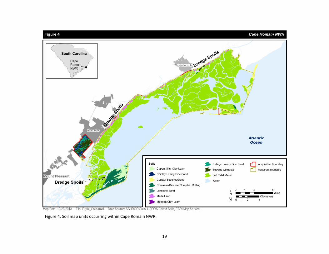
Soils of the South Carolina coastal region are formed from materials that were deposited during the various stages of coastal submersion (Hoyt 1968). During each stage of submersion the formation of new lagoons, marshes, and barrier islands promoted sorting and mixing of these coastal deposits. As the sea retreated during the Late Pleistocene, soil forming processes began to develop the soils we observe today. These soils vary from sand-clay mixtures with distinct horizon development to soils of predominantly quartz sand with indistinct horizon development. Most barrier island soils and marshland soils are of more recent origin, having been laid down during the Holocene period within the last 3,500 years (Hoyt 1968, Riggs et al. 2011). The four major soil associations in the refuge vicinity include tidal marsh, soft; the Crevasse-Dawhoo complex, rolling; Capers silty clay loam; and coastal beaches and dune land (USFWS 2010b, Figure 4). The majority of the land area of the refuge consists of soft tidal marsh with surface soils composed of soft clay, clay loam, muck or peat underlain by a soft, finely-textured clayey material that is permanently saturated. These soils contain sulfide that oxidizes to form sulfuric acid if the land is drained. The Crevasse-Dawhoo complex is associated with ridges ranging from about 5 to 15 feet in height and 25 to 60 feet in width separated by troughs ranging from 10 to 40 feet in width. Within the refuge, the Crevasse-Dawhoo complex occurs on Bulls Island, covering the southern edge and much of the eastern half of the island. Crevasse soils are excessively drained, sandy soils on ridges, while Dawhoo soils are poorly drained sandy soils in troughs. The Capers series consists of very deep, very poorly drained and very slowly permeable soils occurring in tidal marshes. On the refuge Capers clay silty loam occurs on Bulls Island, Cape Island and the western edge of the refuge. Coastal beaches and dune land soils are fine sands. Beach shorelines are flooded twice daily, while the loosely-packed dune sands remain dry (Miller 1971).

4.5 Hydrologic Setting

The National Watershed Boundary Dataset (WBD) divides the landscape into nested hydrologic units (HUs) at progressively finer spatial scales: region, subregion, basin, subbasin, watershed, subwatershed. Each HU is identified by a unique name and a hierarchical numeric code, known as a hydrologic unit code (HUC), ranging from 2 digits at the broadest scale to 12 digits at the finest scale. Cape Romain NWR is located within the Bulls Bay (03050209) hydrographic subbasin of the Edisto-South Carolina Coastal basin (030502), which consists of several adjacent drainages that lie entirely within the Coastal Plain physiographic province (Figure 1 and Figure 2). However, the geomorphology and coastal processes at Cape Romain (see Section 4.3.2) are affected by the Santee and Pee Dee Rivers to the northeast. Prior to dam construction and diversion of river flows for hydropower, the Santee River had the fourth highest discharge rate of the rivers located on the east coast of the U.S. (Kjerfve 1976, Hockensmith 2004). The lower Santee River is bifurcated about 15 miles inland of the delta front, with about three-quarters of the discharge flowing down the north channel (Hayes and Michel 2008). The south and north channels enter the Atlantic Ocean about five and seven miles northeast of the northeastern boundary of the refuge, respectively, while the mouth of the Pee Dee River is about 6 miles farther to the northeast (Figure 1, Figure 2).

19

Figure 4. Soil map units occurring within Cape Romain NWR.

20

4.6 Historical Landscape Changes

4.6.1 Hydrologic Alterations

Extensive clearing of coastal swamp lands for rice plantations occurred in the estuaries and deltas of all the major coastal rivers of South Carolina within the zone of tidal influence (but above the upper limit of saltwater incursion) beginning in the late 1600s, converting the cypress-tupelo swamp that covered much of the lower delta areas to farmland and altering the natural hydrology. These tidal rice fields could be flooded with freshwater at high tide during the growing season and drained on a falling tide for harvest. Rice growing declined in importance following the Civil War due to the loss of slave labor and other economic changes (SCDNR 2000, Hayes and Michel 2008).

Between 1793 and 1800, the 22-mile long Santee Canal was constructed connecting the Santee and Cooper rivers to allow barge transportation between the port of Charleston and inland markets. The canal was abandoned circa 1855 (SCDAH 1979). Because it was operated solely for navigation and had numerous locks, it is unlikely that the canal ever had a very significant effect on streamflow and sediment supply in the Santee and Cooper rivers.

Nearly a century later, a much more ambitious engineering project profoundly altered the hydrology of the Santee River. Between 1939 and 1941, the Santee-Cooper Project created Lake Marion on the Santee River by Wilson Dam and Lake Moultrie in the headwaters of the Cooper River, impounded by Pinopolis Dam and associated dikes (Patterson et al. 1996). According to Patterson et al., approximately 15,000 cubic feet per second (cfs) or 80 percent of the long-term average discharge of the Santee River was diverted into Lake Moultrie, with a minimum flow of 500 cfs released through Wilson Dam, along with that portion of peak flows exceeding 30,000 cfs. Hockensmith (2004) reports a somewhat greater reduction in flow, from 18,500 to 2,600 cfs (86 percent). The Santee-Cooper dam currently operates in accordance with a license and settlement agreement issued by the Federal Energy Regulatory Commission in 2007 (FERC 2007).

The Santee-Cooper flow diversion had the unintended effect of greatly increasing sedimentation in Charleston Harbor, a major commercial and naval port at the mouth of the Cooper River. To reduce the problem of sedimentation in Charleston Harbor, a 12-mile long Rediversion Canal with a hydroelectric dam (St. Stephen Dam) was constructed from Lake Moultrie to a point on the Santee River 37 miles downstream of Wilson Dam, becoming operational in 1985. Since 1985, a daily average flow of 4,500 cfs is released into the Cooper River through the hydropower turbines at Pinopolis Dam, while the remaining flow entering Lake Moultrie is rediverted to the Santee River (Hockensmith 2004).

The reduced flows in the Santee River following its diversion in 1941 had a profound effect on salinity in the Santee Delta, causing average salinity at the mouth of the estuary to increase from <1 milligrams per liter (mg/L) pre-diversion to 20-24 mg/L post-diversion, leading to extensive conversion of freshwater marsh to brackish and saltwater marsh (Gordon et al. 1989). A lucrative shellfish industry (hardshell clams and oysters) became established in the delta following the diversion (Kjervfe 1976). Freshwater conditions returned to the Santee Delta following the rediversion, but not to the level that existed prior to dam construction (Hayes and Michel 2008).

The increased salinity in the Santee Delta following the completion of the Santee-Cooper Project in 1941 appears to have had a significant adverse impact on the refuge. The refuge’s 1942 annual narrative report indicated that waterfowl were scarce on the refuge and throughout the immediate locality and suggested that the cause was due in part, if not entirely, to the intrusion of saltwater in the Santee Delta marshes (USFWS 1942). At the end of December 1942, refuge staff estimated that 20,000 waterfowl

21

were using the refuge, compared to 32,000 for the same period during the preceding season. Of that number, approximately 12,500 ducks were using the northern marshes, described as a huge decrease over preceding years and “probably due to salt water intrusion in the lower Santa Delta region.” The following year the narrative indicated that “Many waterfowl using the northern marshes of the Refuge are dependent on the lower Santee Delta for food. This is the second year of operation for the Santee-Cooper Power Project and the intrusion of salt water in the lower Santee area has had serious effects on waterfowl food plants. Some improvement may take place when the brackish water zone becomes revegetated” (USFWS 1943).

Another engineering project that profoundly affected the hydrology in the vicinity of the refuge was the construction of the AIW. Excavation of the section of the AIW adjacent to the refuge began in the early 1900s, and after several phases of construction in which portions of the route were altered and the canal was widened and deepened, it was completed along its current route by 1940 to a uniform dimensions of 90 feet wide by 12 feet deep (Lewis undated, Mathews et al. 1980). Easements alongside the canal were designated for disposal of dredge spoils from the construction and maintenance of the AIW. In South Carolina, dredge spoils were commonly disposed of within diked enclosures, a practice which completely destroys the previous salt marsh habitat in these areas (Mathews et al. 1980). Dredge spoils piles (both diked and undiked) along the northwestern boundary of the refuge bordering the AIW are visible in aerial imagery and are shown as areas of “made land” in Figure 4.

The AIW has significantly altered the hydrology of the northwestern boundary of the refuge that was previously connected to the mainland by cutting off freshwater inflows via both overland flow and shallow groundwater discharge. Although pre-construction data are not available, the tidal marsh and adjacent estuaries that comprise the majority of the refuge would likely have experienced a lower range of salinity values before they were hydrologically isolated from the mainland by the construction of the AIW than they do today. According to local shellfish harvesters, the changes to the freshwater and sediment discharge from the Santee River have affected the location and quantity of oyster reefs in the northern end of the refuge (Sarah Dawsey, personal communication, January 28, 2013).

The hydrology of Bulls Island has been extensively altered by human inhabitants and management activities since the early 20th century. A review of the 1875 U.S. Coast Survey maps for Bulls Island (Appendix I) reveals that in the mid-1870s, Jacks Creek was tidal and surrounded by an open embayment of tidal marsh subject to tidal inflow and outflow via the north end of the island. On the south end of the island, the 1875 maps depict open/unvegetated areas immediately north and south of Avenue Road (now Beach Road) in the vicinity of present day Lower Summerhouse and House Pond. These areas were possibly agricultural fields when people lived on the island. Moccasin Pond, New Pond, and Pools 1, 2, and 3 were fingers of the Jacks Creek tidal embayment. A subsequent 1919 U.S. Geological Survey (USGS) topographic map of Bulls Island similarly depicted these areas as tidal marsh. This map also shows two small impoundments at the current locations of House and Big Ponds connected by a narrow waterway.

The hydrology of the Jacks Creek embayment was dramatically altered shortly after Gayer Dominick donated Bulls Island to the US Government in 1936 and the island became part of the refuge. The following year a Civilian Conservation Corps (CCC) camp was established on the island, and within two years the 800-acre Jacks Creek impoundment was created with a perimeter dike along the east side of the Island. (During that same period, the CCC constructed an experimental, and ultimately unsuccessful, groin on the northeastern shoreline of the island to address erosion.) Subsequent storm damage, dike repairs, and construction of new dikes to create small impoundments (Pools 1, 2 and 3) in fingers of the former Jacks Creek embayment reduced the size of Jacks Creek impoundment in stages to its current

22

485 acres. Additional details on the history and current status of managed wetland impoundments and dikes at the refuge are provided in Sections 5.1.4, 5.2.4, and Appendix E.

4.6.2 Development and Climate Change Impacts on Coastal Processes

The hydrologic alterations discussed in the preceding section also profoundly impacted sediment transport and delivery. Following the completion of the Santee-Cooper project in 1941, most of the Santee River delta front began eroding rapidly, primarily as a result of the decreased supply of sediment (Morton and Miller 2005, Hayes and Michel 2008, p. 164). Hayes and Michel (2008, p. 174) also suggest that the damming of the Santee River likely contributed to accelerated erosion at Cape Romain (i.e., Cape and Lighthouse Islands). Following the rediversion in 1985, Hayes and Michel (2008, p. 163) note the development of a large swash bar at the mouth of the North Santee River that “probably derived much of its sand from the revitalized river.” However, this sand likely represented material remobilized from upper delta plain and the riverbed downstream of the reservoirs. Patterson et al. (1996) estimated that for the period 1983-85, lakes Marion and Moultrie combined trapped approximately 79% of the total estimated sediment influx of 825,000 tons per year. Hence even after completion of the rediversion project, sediment supply to the Santee River delta (and in particular the supply of sand, for which trapping efficiency is likely close to 100%) remains only a small fraction of the pre-diversion total.

In addition, dredging to maintain Georgetown Harbor has also greatly reduced sediment discharge from Winyah Bay and the Pee Dee River basin. Dredging first began in 1885 to create a 15-foot deep shipping channel, which was subsequently deepened to 19 feet in 1912 and 27 feet in 1947. Following the deepening of the harbor to 27 feet, annual maintenance dredging for the Georgetown Harbor Project increased nearly fourfold to more than 1.4 million cubic yards (1.07 million m3; Mathews et al. 1980). Dredging of Georgetown Harbor, in combination with the north and south jetties constructed in the early 1900s to protect the entrance to Winyah Bay, blocked longshore sediment transport and have effectively cut off the sediment supply from the Pee Dee River basin that previously would have been available to nourish the barrier islands at Cape Romain NWR north of Bulls Bay.

A recent geospatial analysis by Refuge Biologist Dan Ashworth characterized changes in the area and shape of the refuge’s four major barrier islands (Bulls, Cape, and Lighthouse Islands and Raccoon Key) since 1875 using U.S. Coast Survey maps for 1875 and 1929 and aerial imagery from 1949 to 2011 (Appendix D). Overall, the geospatial analysis revealed a net decrease in island area of 321 acres (6%) at Bulls Island, 2,201 acres (51%) at Raccoon Key, and 42 acres (5%) at Cape Island over the entire 136-year period, while Lighthouse Island increased in area by 459 acres (57%) over the same period. Combined, the area of these four barrier islands decreased by 2,105 acres (19%) from 1875 to 2011 (Figure 5). The rate of land loss accelerated after the early 1950s, following completion of the Santee-Cooper Project in 1941, with the average annual rate increasing more than fourfold from 6.3 acres per year for the period 1875-1949 to 26.4 acres per year during 1949-2011.

The analysis revealed distinct patterns of erosion and accretion since 1875, with the different islands following different trajectories. During the 136-year period, the greatest losses from erosion have occurred on the south-facing shoreline of Raccoon Key and the Sandy Point peninsula, where 2,230 acres have been lost (Figure 5). On Bulls Island, erosion has taken 334 acres on the northeast shoreline while the southeastern shoreline has alternately accreted and eroded. The most dramatic changes have occurred at Cape Island, which in effect has migrated northward by nearly its original length, losing 687 acres on the south end and east-facing shoreline while adding 621 acres on the north end of the island.

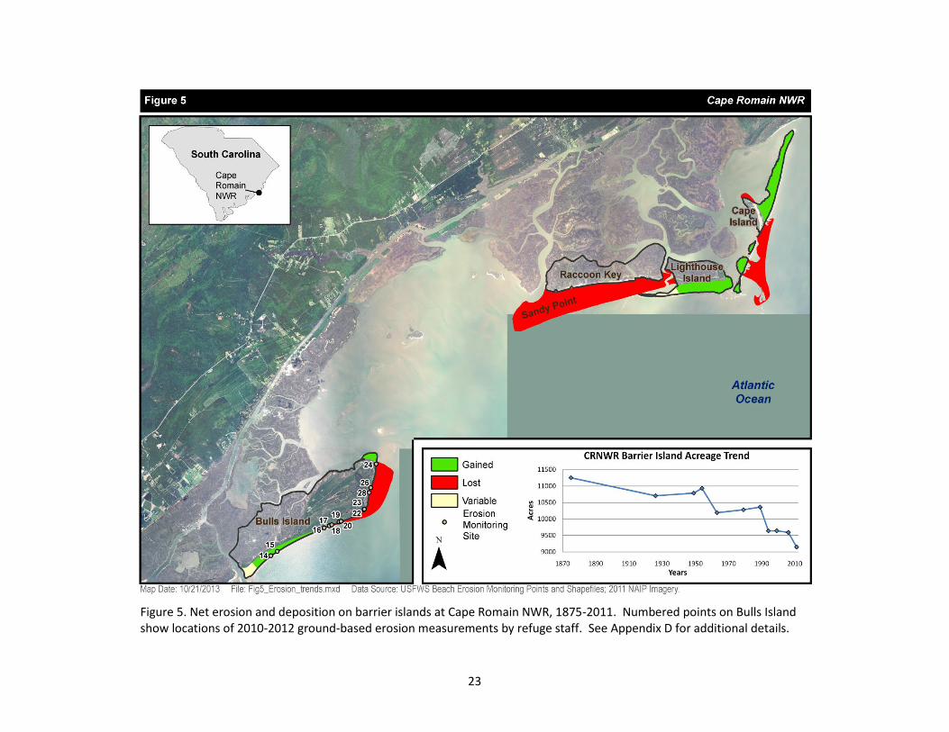
23

Figure 5. Net erosion and deposition on barrier islands at Cape Romain NWR, 1875-2011. Numbered points on Bulls Island show locations of 2010-2012 ground-based erosion measurements by refuge staff. See Appendix D for additional details.

24

The greatest annual rate of loss on Raccoon Key, Lighthouse Island, and Bulls Island occurred in the period 1989 to 1994 when Bulls Island, Raccoon Key, and Lighthouse Island lost an average 44, 43, and 34 acres per year, respectively. In contrast, the greatest annual rate of loss on Cape Island occurred during the period 2006 to 2011 when Cape Island lost an average of 52 acres per year. Presumably, the reason that three of the four main barrier islands exhibited the greatest annual erosion rate for the 1989-1994 period was that Hurricane Hugo made landfall on the refuge in 1989 (subsequent to the 1989 imagery), causing severe erosion and major breaches in the dikes for Jacks Creek and Upper Summerhouse Pond (USFWS 1989). The imagery-based analysis cannot determine what proportion of the erosion for the 1989-1994 is attributable to Hugo; however, in recent years refuge staff have witnessed ongoing erosion each year with punctuated losses caused by intense storm events such as hurricanes, tropical storms, or nor’easters. Ground-based monitoring conducted from 2010 to 2012 at the locations shown in Figure 5 found erosion rates ranging from 5 to more than 25 ft/yr on Bulls Island (Appendix D).

Another indicator of the long-term persistence of shoreline erosion on Bulls Island comes from the 1938 Refuge Narrative Report (USDA-BBS 1938), which describes a project undertaken by the Civilian Conservation Corps camp on Bulls Island to control shoreline erosion. They harvested pine trees on the island to build groins on the northeastern shoreline. The groins were built perpendicular to the shoreline at intervals of approximately 200 feet and extended from eight feet above mean low water to the mean low water mark. The lumber and round timber piles were jetted deep into the sand on the beach, fitted precisely, and then securely nailed and bolted together. The experiment was unsuccessful, as erosion continued following the construction of the groins, and today no evidence remains of their presence on the shoreline.

Erosion of the barrier islands has sometimes resulted in the exposure and of vulnerable salt marsh to the erosive forces of tides and wave action, leading to accelerated loss of salt marsh habitat. For example, after 2009, when the last remnant of Sandy Point (originally attached to the southwest corner of Raccoon Key) eroded and became submerged, salt marsh to the north and west began to rapidly erode, leading to the loss of an approximately 120-acre unnamed island.

In a recent study conducted at the refuge using aerial imagery and field observations, Hughes et al. (2009) reported on tidal creeks that are rapidly incising headward into the marsh platform at an average rate of about 1.9 m/yr. Extrapolating backward in time from 1968 (the earliest imagery they found of sufficient quality to measure channel positions) and assuming a constant incision rate, Hughes et al. (2009) reported that their data suggest that channel incision began around 1940, coincident with the closure of Wilson Dam on the Santee River. However, Hughes et al. point to an elevated rate of local relative sea-level rise as the primary likely cause of channel incision, with decreased sediment supply due to damming of the Santee River as a potential exacerbating factor.

The degree to which the greatly reduced sediment delivery by the Santee River following the closure of Wilson Dam contributed to the observed channel incision into the marsh platform and increased rates of barrier island erosion is uncertain. As noted above and discussed further in Section 4.7.2, elevated local relative sea-level rise rates likely also contribute to (and may be the primary cause of) the observed tidal marsh channel incision and accelerated loss of land area from the barrier islands. Satellite data show global SLR has accelerated over the past 15 years, but at highly variable rates on regional scales (CCSP 2009). Burkett and Davidson (2012) estimate that the global average rate of SLR has increased from 1.7 mm/yr during the 20th century to over 3 mm/yr in the past 20 years.

In addition, the relative importance of Santee delta sediments to the barrier islands at Cape Romain is unknown. While it is likely that the Santee delta has been a source of sediments for the barrier islands north of Bulls Bay, the presence of an open bay would disrupt longshore transport of sediment

25

southward to Bulls Island (Hayes and Michel 2008). Hayes and Michel (2008, p. 130) point to a submerged delta lobe of the ancestral Santee River offshore of Bulls Island as a likely source of the sediment that built Bulls Island and the barrier islands to the south, and sandy shallow shoal deposits offshore of Cape Romain proper (i.e., Cape and Lighthouse Islands) could be a source of sediments for the northern islands. Finally, the dynamics of accretion and erosion at the individual barrier islands (see Appendix D) is too complicated to be explained by a simple decrease in sediment supply. For example, while Raccoon Key lost half its area between 1875 and 2011 (Figure 5), neighboring Lighthouse Island grew by a similar amount and Cape Island migrated northward. This is consistent with the observation by Hayes and Michel (2008) that sediment transport along the northeastern flank of Cape Romain is northward, counter to the dominant southwestward transport direction along the South Carolina coast. This divergent pattern of sediment transport (northward along Cape Island and westward along Lighthouse Island and Raccoon Key) is clearly visible in an annual timelapse animation based on Landsat imagery from 1984-2012 that can be viewed on the Google Earth Engine website at the following url: http://earthengine.google.org/#timelapse/v=33.00952,-79.51742,10.508,latLng&t=0.07.

4.7 Climate Change

As discussed in the preceding section, climate change (and sea-level rise in particular) is already a key stressor affecting Cape Romain NWR and its water resources. This section discusses projected future climate change and its likely impacts on the refuge.

4.7.1 Climate Change Projections

By the last decade of the 21st century, global average surface temperature is projected to rise by 2.8 °C (likely range: 1.7-4.4 °C) under the A1B (moderate) emissions scenario and 3.4 °C (likely range: 2.0-5.4 °C) under the A2 (high) emissions scenario relative to a 1980-1999 baseline (IPCC 2007). Based on the ensemble average of downscaled projections from 15 climate models obtained via the Climate Wizard website (http://www.climatewizard.org/; Girvetz et al. 2009), however, the increase in estimated annual temperature for the same period at Cape Romain under the A2 scenario is only about 1.4 °C, less than half the global average, with summer and fall temperatures increasing by 0.3-0.4 °C more than winter and spring temperatures (Figure 6a). While individual model predictions vary, they generally show the same seasonal pattern and agree fairly closely on the magnitude of the overall increase in mean temperature, with a range of only about 0.6 °C between the 10th and 90th percentile model predictions.

Climate models show much less agreement on future precipitation, with individual models diverging widely in their predictions in both the direction and magnitude of likely changes. The median prediction is for a modest increase of just under 50 mm (about 2 inches), 3.7% of the current normal annual precipitation total (53.23 inches or 1352 mm; Table 1), but the predictions range from a decrease of nearly 70 mm to an increase of more than 80 mm (Figure 6b). There is a particularly high degree of uncertainty about both the direction and magnitude of likely changes in summer precipitation, but the models generally agree in predicting a small decrease in spring precipitation and a small increase in fall precipitation.

Potential evapotranspiration (PET) is predicted to increase by 85 to 115 mm (3.3-4.5 in.) annually due to increased temperatures, with the bulk of the increase (40-60 mm or 1.6-2.4 in.) occurring in the summer months (Figure 6c), which could lead to increased moisture stress for plants and decreased water availability for management of the refuge’s freshwater impoundments on Bulls Island during the summer and fall. These predicted trends suggest a continuation of the historical trends exhibited by pan evaporation data (Table 2). Climatic moisture deficit, a metric quantifying potential moisture stress (calculated as monthly PET minus precipitation, with a value of zero for months where precipitation is

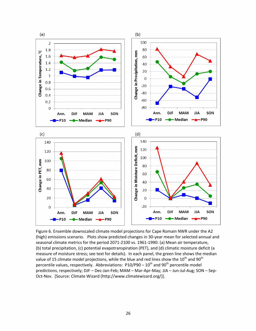
http://earthengine.google.org/#timelapse/v=33.00952,-79.51742,10.508,latLng&t=0.07

http://www.climatewizard.org/

26

Figure 6. Ensemble downscaled climate model projections for Cape Romain NWR under the A2 (high) emissions scenario. Plots show predicted changes in 30-year mean for selected annual and seasonal climate metrics for the period 2071-2100 vs. 1961-1990: (a) Mean air temperature, (b) total precipitation, (c) potential evapotranspiration (PET), and (d) climatic moisture deficit (a measure of moisture stress; see text for details). In each panel, the green line shows the median value of 15 climate model projections, while the blue and red lines show the 10th and 90th percentile values, respectively. Abbreviations: P10/P90 – 10th and 90th percentile model predictions, respectively; DJF – Dec-Jan-Feb; MAM – Mar-Apr-May; JJA – Jun-Jul-Aug; SON – Sep-Oct-Nov. [Source: Climate Wizard (http://www.climatewizard.org/)].

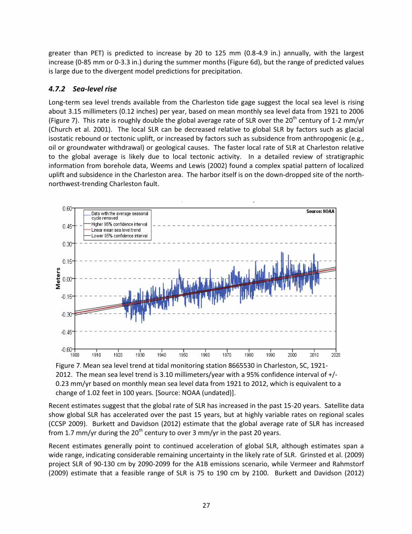
27

greater than PET) is predicted to increase by 20 to 125 mm (0.8-4.9 in.) annually, with the largest increase (0-85 mm or 0-3.3 in.) during the summer months (Figure 6d), but the range of predicted values is large due to the divergent model predictions for precipitation.

4.7.2 Sea-level rise

Long-term sea level trends available from the Charleston tide gage suggest the local sea level is rising about 3.15 millimeters (0.12 inches) per year, based on mean monthly sea level data from 1921 to 2006 (Figure 7). This rate is roughly double the global average rate of SLR over the 20th century of 1-2 mm/yr (Church et al. 2001). The local SLR can be decreased relative to global SLR by factors such as glacial isostatic rebound or tectonic uplift, or increased by factors such as subsidence from anthropogenic (e.g., oil or groundwater withdrawal) or geological causes. The faster local rate of SLR at Charleston relative to the global average is likely due to local tectonic activity. In a detailed review of stratigraphic information from borehole data, Weems and Lewis (2002) found a complex spatial pattern of localized uplift and subsidence in the Charleston area. The harbor itself is on the down-dropped site of the north-northwest-trending Charleston fault.

Recent estimates suggest that the global rate of SLR has increased in the past 15-20 years. Satellite data show global SLR has accelerated over the past 15 years, but at highly variable rates on regional scales (CCSP 2009). Burkett and Davidson (2012) estimate that the global average rate of SLR has increased from 1.7 mm/yr during the 20th century to over 3 mm/yr in the past 20 years.

Recent estimates generally point to continued acceleration of global SLR, although estimates span a wide range, indicating considerable remaining uncertainty in the likely rate of SLR. Grinsted et al. (2009) project SLR of 90-130 cm by 2090-2099 for the A1B emissions scenario, while Vermeer and Rahmstorf (2009) estimate that a feasible range of SLR is 75 to 190 cm by 2100. Burkett and Davidson (2012)

Figure 7. Mean sea level trend at tidal monitoring station 8665530 in Charleston, SC, 1921-2012. The mean sea level trend is 3.10 millimeters/year with a 95% confidence interval of +/- 0.23 mm/yr based on monthly mean sea level data from 1921 to 2012, which is equivalent to a change of 1.02 feet in 100 years. [Source: NOAA (undated)].

28

report that recent studies suggest high confidence (>9 in 10 chance) that global mean sea level will rise 0.2 to 2 meters by the end of this century. Additionally, land subsidence occurring along the southeast Atlantic coast will increase the effects of sea-level rise in this region.

Rising sea levels inundate wetlands and lowlands, accelerate coastal erosion, exacerbate coastal flooding, threaten coastal structures, raise water tables, and increase the salinity of rivers, bays, and aquifers (Barth and Titus 1984, CCSP 2009, Williams and Gutierrez 2009). Coastal development and natural coastal processes also contribute to these impacts (Williams and Gutierrez 2009). For coastal areas that are vulnerable to inundation by sea-level rise, elevation is generally the most critical factor. In sandy shore environments it is virtually certain that coastal headlands, spits, and barrier islands will erode at a faster pace. Sea-level rise by 2 to 7 mm per year will likely cause some barrier islands to cross a threshold where rapid migration or segmentation will occur (CCSP 2009).

The long term stability of salt marsh ecosystems is dependent upon interactions among sea level, land elevation, primary production of the vegetation, and sediment accretion that regulates the elevation of the sediment surface toward equilibrium with mean sea level. The equilibrium is adjusted upward by increased production of the vegetation and downward by an increasing rate of relative sea-level rise (RSLR). However, adjustments in marsh surface elevation are slow in comparison to interannual anomalies and long-period cycles of sea level, which results in significant variation in annual primary productivity (Morris et al. 2002). A theoretical model developed by Morris et al. predicts that the system will be stable against changes in relative mean sea level when surface elevation is greater than what is optimal for primary production. When surface elevation is less than optimal, the system will be unstable. The model predicts that there is an optimal rate of RSLR at which the equilibrium elevation and depth of tidal flooding will be optimal for plant growth, and that this optimal RSLR rate represents an upper limit of marsh stability, because at higher rates of RSLR the plant community cannot sustain an elevation that is within its range of tolerance. Morris et al. (2002) conclude that “for estuaries with high sediment loading, such as those on the southeast coast of the United States, the limiting rate of RSLR was predicted to be at most 1.2 cm/yr, which is 3.5 times greater than the current, long-term rate of RSLR.”

As noted in Section 4.6.2, a recent study at Cape Romain NWR reported that tidal creeks are rapidly incising headward into the marsh platform at an average rate of about 1.9 m/yr (Hughes et al. 2009). Extrapolating backward in time from 1968 and assuming a constant incision rate, Hughes et al. reported that their data suggest that channel incision began around 1940. They proposed that the growth of creeks in this region was a manifestation of a high RSLR rate (> 3.2mm/yr) that exceeded the sediment accretion rate, forcing the marsh platform into a state of disequilibrium. The formation and rapid extension of creeks in this region represents an alternative scenario to marsh submergence as the morphological response of marshes to future high rates of SLR. The initiation of channel incision circa 1940 coincides with both reduced sediment supply to the Santee delta following dam construction and rapid local RSLR evident in the Charleston tide curve during the 1940s (Figure 7).

Besides marine inundation, low-lying coastal areas may also be vulnerable to groundwater inundation, which is localized coastal-plain flooding due to a rise of the groundwater table with sea level. As sea-level rises, the water table will rise simultaneously and eventually break out above the land surface. Flooding will start sporadically but will be especially intense seasonally when high tide coincides with rainfall events. Rising groundwater levels could cause long-term problems related to water management (aquifer salinization) and infrastructure (flooding) in coastal areas (Rotzoll and Fletcher 2012).

29

4.7.3 SLAMM Modeling

The Sea Level Affecting Marshes Model (SLAMM) attempts to quantify the effects of SLR on coastal wetland habitat using data from National Oceanic and Atmospheric Administration (NOAA) tide gages, NWI maps and USGS digital elevation models. In addition to inundation by rising sea level, the model accounts for other key processes that affect wetland habitat, including horizontal erosion, overwash of barrier islands, and accretion (sedimentation). SLAMM was first applied to the refuge in 2008 (Ehman 2008), then again in 2012 to include LiDAR-derived elevation data for a small portion of the refuge, an updated NWI data layer from 2009 and a scenario of 2 meters of eustatic SLR. SLAMM was used to predict wetland habitat changes on the refuge by 2100 under five SLR scenarios: A1B Mean (0.39 m), A1B Maximum (0.69 m), 1 m eustatic, 1.5 m eustatic and 2 m eustatic (Warren Pinnacle Consulting 2012).

The SLAMM simulation of the refuge suggests that it is fairly resilient to the effects of SLR under the lowest scenario (0.39 m); however, under higher rates of SLR (0.69 to 2 m), the refuge is predicted to lose significant areas of the majority of habitat types (Figure 8, Table 3). Regularly-flooded marsh, the dominant wetland type, is predicted to experience losses of 60-98% under the 0.69 to 2 m scenarios. Under these scenarios, most to nearly all of existing regularly-flooded marsh is predicted to convert to tidal flat by the middle to end of the current century (Figure 8; Warren Pinnacle Consulting 2012), then ultimately to convert to estuarine open water by 2100 under the 1.5 and 2 m SLR scenarios (Table 3).

All model results are subject to uncertainty due to limitations in input data, incomplete knowledge about factors that control the behavior of the system being modeled, and simplifications of the system (EPA 2008). In this instance, the SLAMM model results must be interpreted with caution in the light of serious limitations in the quality of available input data. In particular, LiDAR elevation data were only available for portions of the refuge directly in contact with open ocean (the “coastal strip”); these data were collected in 2000 and 2006. Most of the refuge area was not covered by LiDAR-derived elevation data; for these areas, elevations were based on datasets released between 1942 and 1957 with contour intervals of between 5 and 20 m, resulting in poorly characterized wetland elevations.

As a consequence of this lack of vertical accuracy, the SLAMM elevation pre-processor was used for the entire site. This module assigns elevations for wetlands as a function of the local tide range (Clough et al. 2010). An additional cause of uncertainty within these predictions is the model’s estimation of marsh accretion rates. Vertical marsh accretion rates may react to an increase in sea-level rise due to more frequent inundation and higher sediment trapping within marshes. For this study area, data were available to apply such a feedback to the regularly-flooded marsh wetland category (Warren Pinnacle Consulting 2012). This led to some additional marsh resilience, particularly under the 0.39 m SLR scenario. Future model runs for this site could potentially evaluate the extent of this feedback using additional data, or as part of a model sensitivity or uncertainty analysis.

In addition to poor quality elevation data, the SLAMM simulations relied on outdated NWI land cover data to characterize initial habitat conditions. Refuge staff recently compiled an updated classification of wetland habitat types at the refuge using the Cowardin Classification System method (Cowardin et al. 1979). The results revealed significant differences between existing conditions on the ground and the NWI classification that was used in the SLAMM simulations (Table 5 and Section 5.1.4). These differences were most pronounced for Bulls Island, where all the actively managed impoundments and a large proportion of refuge management activities are located.

Another limitation of the SLAMM model is that it does not capture some coastal processes known to be important at the refuge. For example, SLAMM does not simulate the fragmentation of tidal marsh by rapid headward extension of tidal channels documented at Cape Romain by Hughes et al. (2009).

30

SLAMM also fails to capture important event-scale dynamics that occur during hurricanes and other major storms, such as episodic shoreline erosion, breaching of barrier islands to create new tidal inlets, or breaching dikes surrounding managed impoundments. For example, in the SLAMM simulations for Cape Romain NWR, the impoundments on Bulls Island are assumed to remain protected from the effects of SLR until local SLR exceeds 2 m. However, this assumption is clearly unrealistic, as the seaward dike protecting the Jacks Creek impoundment has already been breached multiple times in the past, most recently in 2008 (Table 11; Appendix E). Currently the toe of this dike is approximately 150 feet from the shoreline at the closest approach, and at current erosion rates of around 10 to more than 25 feet per year (Appendix D) it is expected to fail within the next 5-10 years.

Despite these limitations, the SLAMM model has been used to estimate and refine the impacts of sea-level rise across the coasts of the United States since the 1980s. Hence the SLAMM model results put the issues of sea-level rise at Cape Romain NWR into a larger, landscape level context. However, the lack of accurate, high resolution topographic data for most of the refuge, together with reliance on outdated NWI maps and inability of SLAMM to simulate important processes governing habitat change at the refuge (e.g., barrier island breaching and marsh fragmentation by headward channel extension) seriously limits the utility of the current SLAMM results for refuge planning purposes or for comparisons of likely SLR impacts at Cape Romain NWR versus other coastal refuges or other areas of management concern.

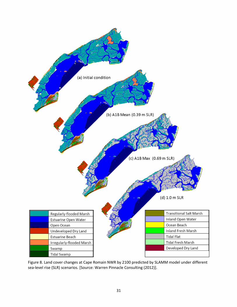
31

Figure 8. Land cover changes at Cape Romain NWR by 2100 predicted by SLAMM model under different sea-level rise (SLR) scenarios. [Source: Warren Pinnacle Consulting (2012)].

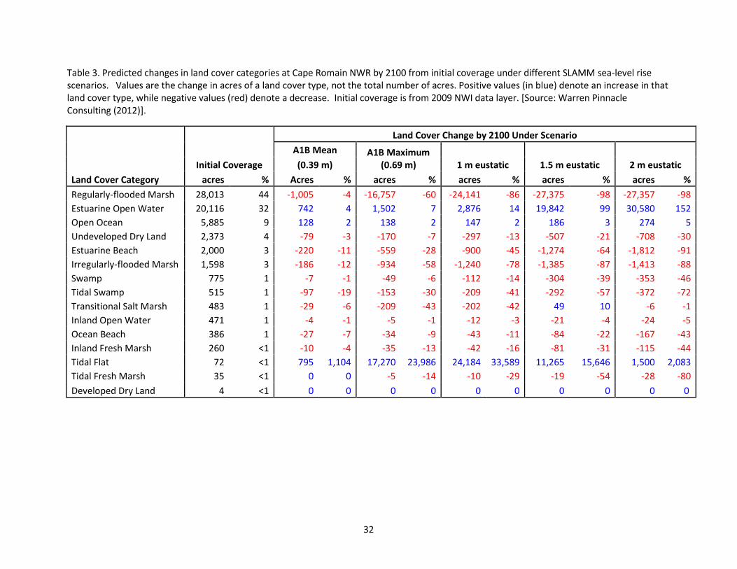
32

Table 3. Predicted changes in land cover categories at Cape Romain NWR by 2100 from initial coverage under different SLAMM sea-level rise scenarios. Values are the change in acres of a land cover type, not the total number of acres. Positive values (in blue) denote an increase in that land cover type, while negative values (red) denote a decrease. Initial coverage is from 2009 NWI data layer. [Source: Warren Pinnacle Consulting (2012)].

Initial Coverage

Land Cover Change by 2100 Under Scenario

A1B Mean A1B Maximum (0.69 m) 1 m eustatic 1.5 m eustatic 2 m eustatic (0.39 m)

Land Cover Category acres % Acres % acres % acres % acres % acres %

Regularly-flooded Marsh 28,013 44 -1,005 -4 -16,757 -60 -24,141 -86 -27,375 -98 -27,357 -98

Estuarine Open Water 20,116 32 742 4 1,502 7 2,876 14 19,842 99 30,580 152

Open Ocean 5,885 9 128 2 138 2 147 2 186 3 274 5

Undeveloped Dry Land 2,373 4 -79 -3 -170 -7 -297 -13 -507 -21 -708 -30

Estuarine Beach 2,000 3 -220 -11 -559 -28 -900 -45 -1,274 -64 -1,812 -91

Irregularly-flooded Marsh 1,598 3 -186 -12 -934 -58 -1,240 -78 -1,385 -87 -1,413 -88

Swamp 775 1 -7 -1 -49 -6 -112 -14 -304 -39 -353 -46

Tidal Swamp 515 1 -97 -19 -153 -30 -209 -41 -292 -57 -372 -72

Transitional Salt Marsh 483 1 -29 -6 -209 -43 -202 -42 49 10 -6 -1

Inland Open Water 471 1 -4 -1 -5 -1 -12 -3 -21 -4 -24 -5

Ocean Beach 386 1 -27 -7 -34 -9 -43 -11 -84 -22 -167 -43

Inland Fresh Marsh 260 <1 -10 -4 -35 -13 -42 -16 -81 -31 -115 -44

Tidal Flat 72 <1 795 1,104 17,270 23,986 24,184 33,589 11,265 15,646 1,500 2,083

Tidal Fresh Marsh 35 <1 0 0 -5 -14 -10 -29 -19 -54 -28 -80

Developed Dry Land 4 <1 0 0 0 0 0 0 0 0 0 0

33

4.7.4 Storm Frequency and Intensity

In addition to rising sea levels, Cape Romain’s sandy shorelines are greatly influenced by storm events. Even in the absence of any change in storm frequency or intensity, rising sea levels will lead to higher storm surge levels and waves that travel farther inland, likely resulting in greater coastal erosion and damage (Kunkel et al. 2008).

One frequently predicted consequence of global warming is an increase in the intensity of storms and extreme weather events. Holland and Webster (2007) report that tropical cyclone and hurricane frequency in the North Atlantic Ocean over the past century has been characterized by three relatively stable regimes separated by sharp transitions. Each regime has seen 50% more tropical cyclones and hurricanes than the previous regime and is associated with a distinct range of sea surface temperatures (SSTs) in the eastern Atlantic Ocean. Holland and Webster (2007) conclude that the increase in tropical cyclone and hurricane frequency is related to a 0.7 °C increase in sea surface temperatures and is “substantially influenced” by warming attributable to greenhouse gas emissions. A recent assessment by the U.S. Climate Change Science Program similarly found that Atlantic tropical cyclone activity as measured by both frequency and the Power Dissipation Index (PDI, an index that combines storm intensity, duration, and frequency) has increased substantially since about 1970, and that decadal-scale variations in PDI are strongly correlated with decadal-scale variations in tropical Atlantic sea surface temperatures (Kunkel et al. 2008). In contrast, the frequency of ETCs has decreased over the period 1959-1997 for the mid-latitudes (30°-60° N) (while increasing for high latitudes [60°-90°N]). However, ETC intensity has increased over the same period, although the trend is more significant for the high latitudes (p < 0.01) than the mid-latitudes (p < 0.10) (Kunkel et al. 2008).

The high sensitivity of tropical storm and hurricane activity in the Atlantic basin to modest environmental variations suggests the possibility that hurricane activity may be highly sensitive to anthropogenic climate change, though the nature of such changes remains to be determined. However, there is climate model-based evidence that the average climate in the late 21st century will be characterized by higher tropical cyclone potential intensity in most tropical cyclone regions (Gutowski et al. 2008). One study predicted that a CO2-induced tropical sea surface temperature warming of 1.75 °C would yield a 6% increase in maximum surface wind speed (Knutson and Tuleya 2008). With respect to tropical cyclone frequency, while there is recent observational evidence for an increase in the frequency of tropical cyclones in the Atlantic since 1970 as noted above, a confident assessment of future storm frequency cannot be made at this time (Gutowski et al. 2008).

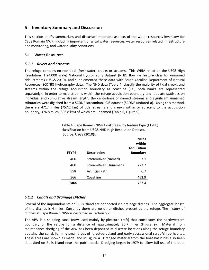
34

5 Inventory Summary and Discussion

This section briefly summarizes and discusses important aspects of the water resources inventory for Cape Romain NWR, including important physical water resources, water resources related infrastructure and monitoring, and water quality conditions.

5.1 Water Resources

5.1.1 Rivers and Streams

The refuge contains no non-tidal (freshwater) creeks or streams. This WRIA relied on the USGS High Resolution (1:24,000 scale) National Hydrography Dataset (NHD) flowline feature class for unnamed tidal streams (USGS 2010), and supplemented these data with South Carolina Department of Natural Resources (SCDNR) hydrography data. The NHD data (Table 4) classify the majority of tidal creeks and streams within the refuge acquisition boundary as coastline (i.e., both banks are represented separately). In order to map streams within the refuge acquisition boundary and tabulate statistics on individual and cumulative stream length, the centerlines of named streams and significant unnamed tributaries were digitized from a SCDNR streambank GIS dataset (SCDNR undated-a). Using this method, there are 471.4 miles (757.2 km) of tidal streams and creeks within or adjacent to the acquisition boundary, 376.8 miles (606.8 km) of which are unnamed (Table 5, Figure 9).

Table 4. Cape Romain NWR tidal creeks by feature type (FTYPE) classification from USGS NHD High Resolution Dataset. [Source: USGS (2010)].

FTYPE Description

Miles within

Acquisition Boundary

460 StreamRiver (Named) 3.1

460 StreamRiver (Unnamed) 273.7

558 Artificial Path 6.7

566 Coastline 453.9

Total

737.4

5.1.2 Canals and Drainage Ditches

Several of the impoundments on Bulls Island are connected via drainage ditches. The aggregate length of the ditches is 4 miles. Currently there are no other ditches present at the refuge. The history of ditches at Cape Romain NWR is described in Section 5.2.3.

The AIW is a shipping canal (now used mainly by pleasure craft) that constitutes the northwestern boundary of the refuge for a distance of approximately 20.7 miles (Figure 9). Material from maintenance dredging of the AIW has been deposited at discrete locations along the refuge boundary abutting the canal, forming small areas of forested upland and early successional scrub/shrub habitat. These areas are shown as made land in Figure 4. Dredged material from the boat basin has also been deposited on Bulls Island near the public dock. Dredging began in 1979 to allow full use of the boat

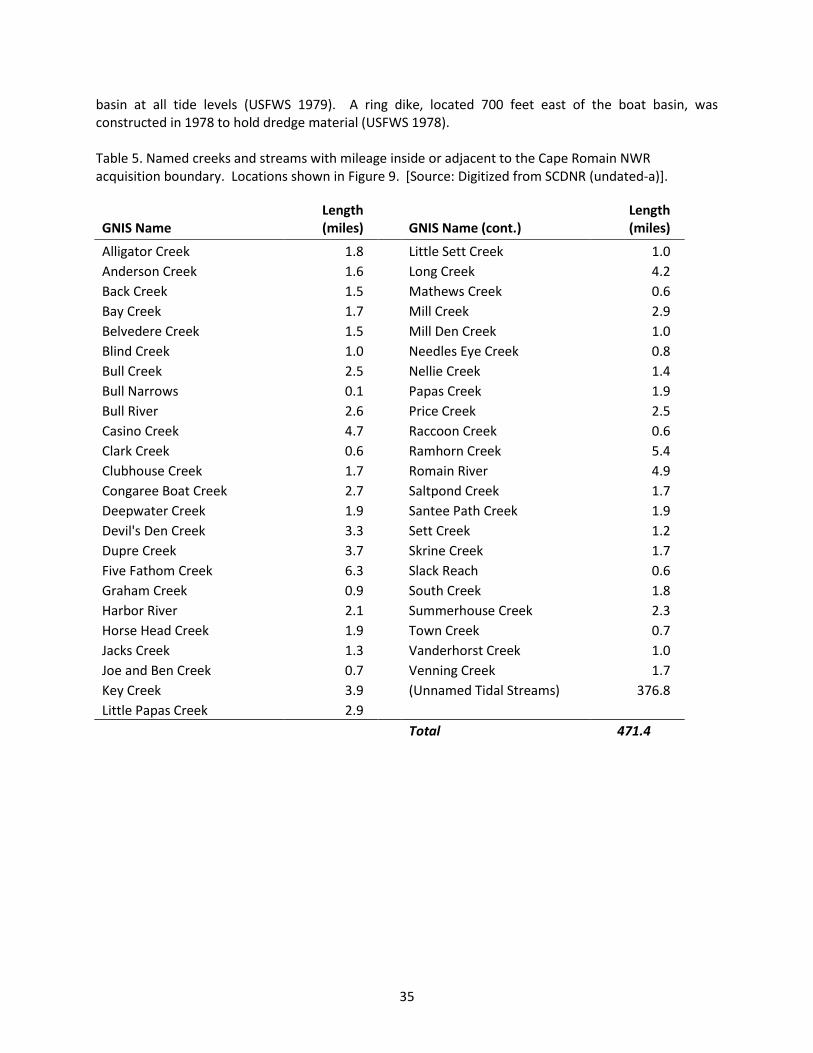
35

basin at all tide levels (USFWS 1979). A ring dike, located 700 feet east of the boat basin, was constructed in 1978 to hold dredge material (USFWS 1978). Table 5. Named creeks and streams with mileage inside or adjacent to the Cape Romain NWR acquisition boundary. Locations shown in Figure 9. [Source: Digitized from SCDNR (undated-a)].

GNIS Name Length (miles)

GNIS Name (cont.)

Length (miles)

Alligator Creek 1.8

Little Sett Creek 1.0

Anderson Creek 1.6

Long Creek 4.2

Back Creek 1.5

Mathews Creek 0.6

Bay Creek 1.7

Mill Creek 2.9

Belvedere Creek 1.5

Mill Den Creek 1.0

Blind Creek 1.0

Needles Eye Creek 0.8

Bull Creek 2.5

Nellie Creek 1.4

Bull Narrows 0.1

Papas Creek 1.9

Bull River 2.6

Price Creek 2.5

Casino Creek 4.7

Raccoon Creek 0.6

Clark Creek 0.6

Ramhorn Creek 5.4

Clubhouse Creek 1.7

Romain River 4.9

Congaree Boat Creek 2.7

Saltpond Creek 1.7

Deepwater Creek 1.9

Santee Path Creek 1.9

Devil's Den Creek 3.3

Sett Creek 1.2

Dupre Creek 3.7

Skrine Creek 1.7

Five Fathom Creek 6.3

Slack Reach 0.6

Graham Creek 0.9

South Creek 1.8

Harbor River 2.1

Summerhouse Creek 2.3

Horse Head Creek 1.9

Town Creek 0.7

Jacks Creek 1.3

Vanderhorst Creek 1.0

Joe and Ben Creek 0.7

Venning Creek 1.7

Key Creek 3.9

(Unnamed Tidal Streams) 376.8

Little Papas Creek 2.9

Total 471.4

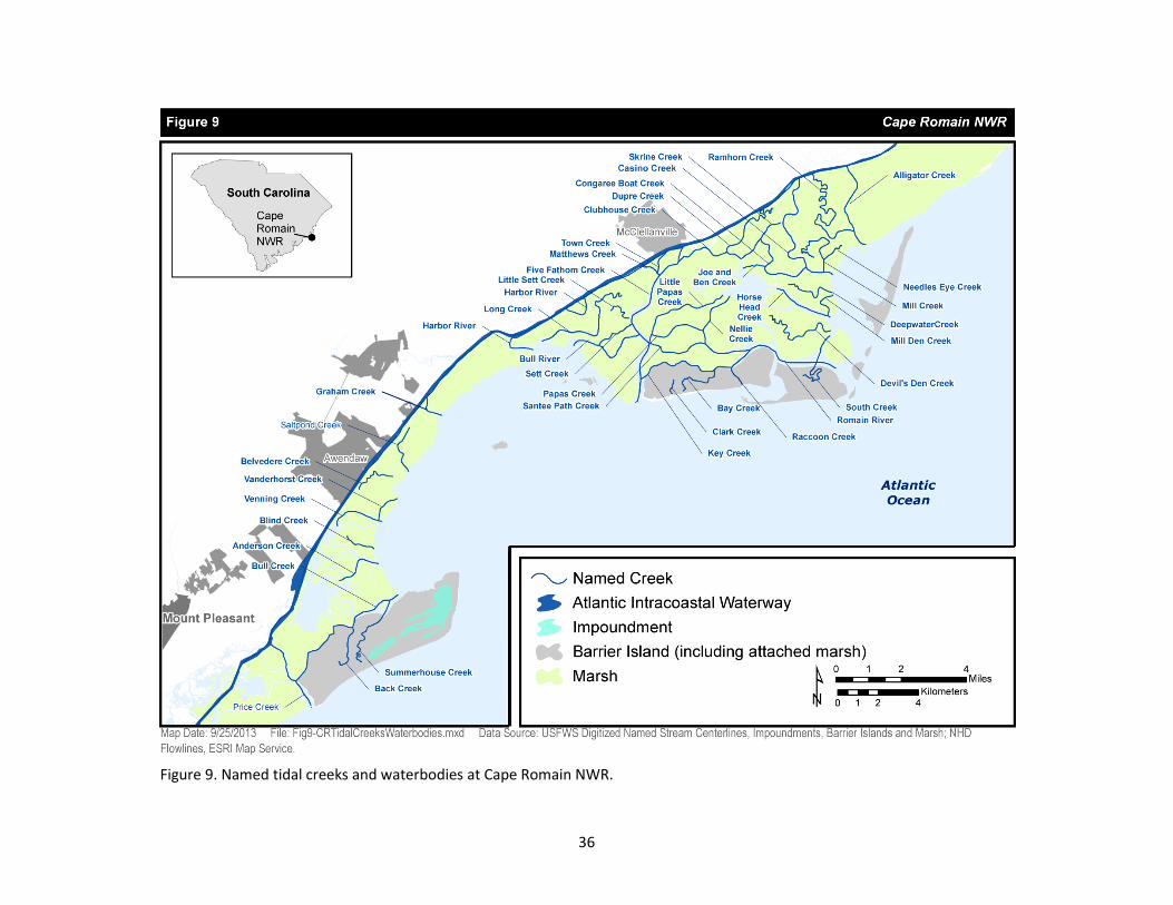
36

Figure 9. Named tidal creeks and waterbodies at Cape Romain NWR.

37

5.1.3 Lakes and Ponds

The NHD identifies 33 unnamed waterbody features (type 390, classified as lake/pond) within the refuge boundaries, ranging in size from less than a tenth of an acre to just over nine acres. The NHD also identifies three named waterbodies which correspond to three of the 10 refuge impoundments (Big Pond, Moccasin Pond and Upper Summerhouse Pond) (Table 6). The acreages given in Table 6 for the three impoundments are all smaller than the values provided by the refuge (Table 8), likely due to the inability of the classification algorithm used by NHD to identify standing water obscured by emergent vegetation or algal blooms (Dan Ashworth, personal communication, January 28, 2013). Note that NHD classifies lakes and ponds differently than the Cowardin Wetland Classification System (Cowardin et al. 1979) discussed in the following section. Under the Cowardin system, Big Pond is classified as freshwater emergent wetland while Moccasin Pond and Upper Summerhouse Pond are classified as estuarine and marine wetlands. An 1875 U.S. Coast Survey map (Appendix I) shows that no lakes or ponds existed on Bulls Island at that time.

Table 6. Acreage of lakes and ponds inside the Cape Romain NWR acquisition boundary. [Source: USGS (2010)].

Pond Name Acres

Big Pond 3.65

Moccasin Pond 6.27

Upper Summerhouse Pond 43.91

33 Unnamed Lakes/Ponds 58.80

Total 112.64

5.1.4 Wetlands

Using the Classification of Wetlands and Deepwater Habitats of the United States (Cowardin et al. 1979), the predominant wetland classes at the refuge are marine and estuarine. After finding NWI maps to be insufficiently accurate and up-to-date for their purposes, refuge staff applied the Cowardin classification method to generate their own wetland landcover map (Figure 10). According to this classification, the refuge (including all areas within the acquisition boundary) consists of 44.39% estuarine and marine wetlands, 44.7% estuarine and marine deepwater aquatic habitat, 4.94% upland or unclassified habitats, 1.73% freshwater forested/shrub-wetlands, and 0.24% freshwater emergent wetlands (Table 7). Although the refuge’s map generally mirrors NWI over most of the refuge area and the relative amounts of most habitat types are quite similar between the two (Table 7), there are significant differences in some areas of management concern for the refuge, particularly on Bulls Island. For example, the NWI classifies some impoundments as emergent wetlands, whereas others are classified as lakes. Also, the NWI data exclude some areas of Cape and Lighthouse Islands that extend beyond the original (and current official) refuge boundary due to accretion in recent years. In addition, the total habitat area differs significantly between the NWI data (62,987 acres) and the refuge’s map (69,586 acres). Therefore, the refuge data are utilized in this report.

38

Table 7. Acres of wetland habitat types within the Cape Romain NWR acquisition boundary delineated by refuge staff using the classification of Cowardin et al. (1979), as shown in Figure 10.Corresponding values obtained from the National Wetland Inventory (NWI) dataset are given for comparison. Note that NWI acre totals are based on the approved acquisition boundary, while the refuge classification includes areas that extend beyond the approved acquisition boundary. [Sources: Cape Romain NWR GIS data and USFWS (undated)].

Habitat Type Refuge Classification NWI Values

Acres % of Total Acres % of Total

Estuarine and marine wetland 33,676 48.39 33,381 53.00

Estuarine and marine deepwater 31,107 44.70 25,164 39.95

Upland or unclassified 3,435 4.94 2,379 3.78

Freshwater forested/shrub wetland 1.201 1.73 1,295 2.06

Freshwater emergent wetland 167 0.24 294 0.47

Lake 0 0 411 0.65

Freshwater pond 0 0 61 0.10

Total 69,586 100.00 62,985 100.00

Table 8. Acreage of impoundments on Bulls Island, Cape Romain NWR. Locations shown in Figure 11. [Source: Cape Romain NWR GIS data].

Name Acres

Jacks Creek 484.8

Moccasin Pond 35.1

New Pond 7.8

Upper Summerhouse Pond 64.5

Lower Summerhouse Pond 57.8

House Pond 13.1

Big Pond 23.9

Pool 1 16.0

Pool 2 29.3

Pool 3 23.8

Total 756.1

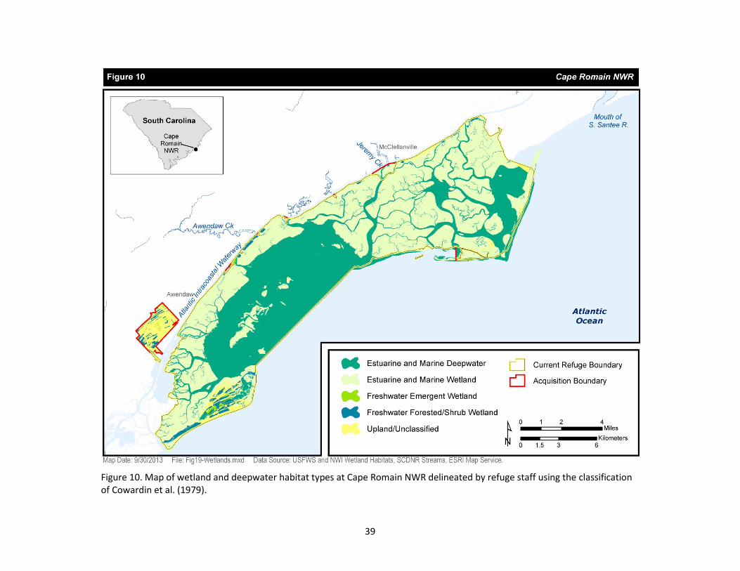
39

Figure 10. Map of wetland and deepwater habitat types at Cape Romain NWR delineated by refuge staff using the classification of Cowardin et al. (1979).

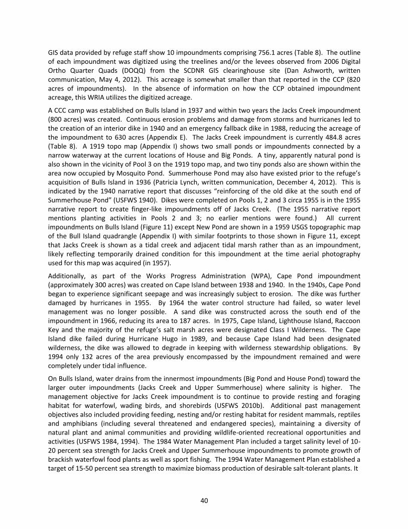
40

GIS data provided by refuge staff show 10 impoundments comprising 756.1 acres (Table 8). The outline of each impoundment was digitized using the treelines and/or the levees observed from 2006 Digital Ortho Quarter Quads (DOQQ) from the SCDNR GIS clearinghouse site (Dan Ashworth, written communication, May 4, 2012). This acreage is somewhat smaller than that reported in the CCP (820 acres of impoundments). In the absence of information on how the CCP obtained impoundment acreage, this WRIA utilizes the digitized acreage.

A CCC camp was established on Bulls Island in 1937 and within two years the Jacks Creek impoundment (800 acres) was created. Continuous erosion problems and damage from storms and hurricanes led to the creation of an interior dike in 1940 and an emergency fallback dike in 1988, reducing the acreage of the impoundment to 630 acres (Appendix E). The Jacks Creek impoundment is currently 484.8 acres (Table 8). A 1919 topo map (Appendix I) shows two small ponds or impoundments connected by a narrow waterway at the current locations of House and Big Ponds. A tiny, apparently natural pond is also shown in the vicinity of Pool 3 on the 1919 topo map, and two tiny ponds also are shown within the area now occupied by Mosquito Pond. Summerhouse Pond may also have existed prior to the refuge’s acquisition of Bulls Island in 1936 (Patricia Lynch, written communication, December 4, 2012). This is indicated by the 1940 narrative report that discusses “reinforcing of the old dike at the south end of Summerhouse Pond” (USFWS 1940). Dikes were completed on Pools 1, 2 and 3 circa 1955 is in the 1955 narrative report to create finger-like impoundments off of Jacks Creek. (The 1955 narrative report mentions planting activities in Pools 2 and 3; no earlier mentions were found.) All current impoundments on Bulls Island (Figure 11) except New Pond are shown in a 1959 USGS topographic map of the Bull Island quadrangle (Appendix I) with similar footprints to those shown in Figure 11, except that Jacks Creek is shown as a tidal creek and adjacent tidal marsh rather than as an impoundment, likely reflecting temporarily drained condition for this impoundment at the time aerial photography used for this map was acquired (in 1957).

Additionally, as part of the Works Progress Administration (WPA), Cape Pond impoundment (approximately 300 acres) was created on Cape Island between 1938 and 1940. In the 1940s, Cape Pond began to experience significant seepage and was increasingly subject to erosion. The dike was further damaged by hurricanes in 1955. By 1964 the water control structure had failed, so water level management was no longer possible. A sand dike was constructed across the south end of the impoundment in 1966, reducing its area to 187 acres. In 1975, Cape Island, Lighthouse Island, Raccoon Key and the majority of the refuge’s salt marsh acres were designated Class I Wilderness. The Cape Island dike failed during Hurricane Hugo in 1989, and because Cape Island had been designated wilderness, the dike was allowed to degrade in keeping with wilderness stewardship obligations. By 1994 only 132 acres of the area previously encompassed by the impoundment remained and were completely under tidal influence.

On Bulls Island, water drains from the innermost impoundments (Big Pond and House Pond) toward the larger outer impoundments (Jacks Creek and Upper Summerhouse) where salinity is higher. The management objective for Jacks Creek impoundment is to continue to provide resting and foraging habitat for waterfowl, wading birds, and shorebirds (USFWS 2010b). Additional past management objectives also included providing feeding, nesting and/or resting habitat for resident mammals, reptiles and amphibians (including several threatened and endangered species), maintaining a diversity of natural plant and animal communities and providing wildlife-oriented recreational opportunities and activities (USFWS 1984, 1994). The 1984 Water Management Plan included a target salinity level of 10-20 percent sea strength for Jacks Creek and Upper Summerhouse impoundments to promote growth of brackish waterfowl food plants as well as sport fishing. The 1994 Water Management Plan established a target of 15-50 percent sea strength to maximize biomass production of desirable salt-tolerant plants. It

41

Figure 11. Impoundments and water management infrastructure on Bulls Island, Cape Romain NWR.

42

no longer included a fishing management goal because after the breach of the Jacks Creek dike in 1988, salinity levels remained too high to support freshwater species (USFWS 1994).

In 2012 the American Reinvestment and Recovery Act (ARRA) funded a project to raise the Big Pond levee and replace or renovate 12 WCS on Bulls Island (Figure 11 and Section 5.2.2). The project improved basic infrastructure for water management capability, resolving one of the many issues that prevent maintenance of optimal habitat conditions for waterfowl. However, other issues limiting habitat management capacity remain. First, management capability is limited by availability of freshwater, which is supplied solely by rainfall and runoff on the island. During dry years there is often insufficient freshwater to maintain desired water levels and habitat conditions in the impoundments, particularly in the late summer and fall. Second, transfer of water between impoundments can only be accomplished passively, by removing or adding flashboard risers at WCS to regulate flow into or out of an impoundment by gravity drainage or tidal influence. Third, the conveyance ditches are in need of clearing and/or re-grading to permit effective water transfer between impoundments. Refuge staff are currently working to clean out the existing channels to enhance conveyance capacity, but accurate information about existing ditch grades and WCS elevations is not currently available.

Insufficient refuge staffing levels present another challenge to maintaining desired habitat conditions in the managed wetland impoundments. Historically, an assistant refuge manager lived full-time on Bulls Island, managing and manipulating water levels to achieve optimum habitat conditions for waterfowl, preparing the impoundments for the waterfowl season, monitoring the success of treatments, and devoting time and attention to the habitat and species. Today the refuge employs only five full-time staff, less than half the number of employees that were on staff ten years ago. There are no staff members living on the island, and visits to the island are not structured around impoundment management. During turtle nesting season from May to October, one refuge staff member or one volunteer is on the island daily to conduct sea turtle recovery activities. Salinities and water levels are recorded once a week throughout the year. Management activities during the summer consist of monitoring the salinity and water levels within the larger brackish impoundments and moving water in or out, dependent on rainfall, attempting to always keep the bottom covered to prevent build-up of sulfuric acid.

5.1.5 Groundwater

A long and complex history of sediment deposition, primarily in response to changes in sea level, has created a sequence of aquifers and low-permeability confining units (Miller 1992, Campbell and Coes 2010). Aucott (1996) identified six major aquifers within the ACP sediments in South Carolina, while Campbell and Coes (2010) developed a more detailed hydrostratigraphy consisting of eight aquifers with seven intervening confining layers. The uppermost aquifer, known as the surficial aquifer, is a water table aquifer consisting of a heterogeneous mix of gravel, sand, silt and clay. The uppermost artesian (confined) aquifer is the Floridan aquifer system, a highly productive aquifer system consisting of limestone and clastic sediments (principally sand) comprising two or three aquifers (depending upon location) and associated confining units (Campbell and Coes 2010). In the vicinity of the refuge, the surficial aquifer is between 10 and 50 feet thick and is underlain by the Gordon aquifer, the lowermost unit of the Floridan aquifer system, which has a thickness between 50 and 100 feet beneath the refuge, increasing toward the west and south. The Gordon aquifer is unconfined north of Bulls Bay, but is overlain by the Middle Floridan confining unit to the south, with the thickness of the confining unit increasing from about 10 feet at the north end of Bulls Bay to over 50 feet at the south end (Campbell and Coes 2010: figures B6, B12, and B18). Three deeper confined aquifers, the Crouch Branch, McQueen Branch, and Charleston aquifers, underlie the refuge vicinity between depths of about 500 to

43

800, 1,000 to 1,200, and 1,600 to 1,800 feet, respectively (Campbell and Coes 2010: figures B21 and B22, B25 and B26, and B29 and B30).

The refuge is located in the Trident Capacity Use Area, one of four designated capacity use areas in the state in which groundwater withdrawals are regulated due to significant drawdowns (Wachob et al. 2009). Major wells in the McClellanville area tapping the Floridan/Tertiary sand aquifer yield 50-200 gallons per minute (gpm) (Wachob et al. 2009). Wells completed in the McQueen Branch and Charleston aquifers yield 500 to 1,500 gpm of soft, sodium bicarbonate-type water. Mount Pleasant Waterworks withdraws water from the Charleston (Middendorf) aquifer, while Georgetown County Water and Sewer withdraws water from the McQueen Branch (Black Creek) aquifer (Bruce Campbell, written communication, June 17, 2013). As of November 2009, well-developed cones of depression around Mount Pleasant and Georgetown (within the Charleston and McQueen Branch aquifers, respectively) extended to the vicinity of the refuge, with potentiometric surface elevations in each of these aquifers between 0 and 25 ft below sea level beneath Bulls Island (Hockensmith 2012a, 2012b). Due to reduced pumping by Mount Pleasant Waterworks in the past five years, the potentiometric surface for the Charleston aquifer would likely be above sea level beneath the refuge at present (Bruce Campbell, written communication, June 17, 2013), although local monitoring data are not available. Prior to development, potentiometric surface elevations in the Charleston and McQueen Branch aquifers in the vicinity of Bulls Island were 75-100 ft and 50-75 ft above sea level, respectively (Aucott and Speiran 1985).

A shallow cone of depression has existed in part of the Floridan aquifer system at Charleston for many years, so slow, lateral saltwater intrusion is likely (Harwell et al. 2004). Harwell et al. also note that lateral intrusion occurs along the coast of Charleston County where pumping from the Middendorf aquifer system (which underlies the Floridan aquifer system and is equivalent to the Charleston acquifer of Campbell and Coes [2010]) captures brackish water that lies in the system offshore. Due to the system’s low hydraulic conductivity and the broad, diffuse nature of the brackish-water front, however, this is not a significant problem (Harwell et al. 2004).

Groundwater is not currently used for habitat management on the refuge, nor has it been used historically, although there were some apparently unsuccessful attempts to do so. The refuge’s annual narrative for 1938 mentions that a test well was drilled on Bulls Island for the purpose of supplying water to the ponds during dry seasons. It was drilled to a depth of 450 feet and pierced a water-bearing stratum at 200 feet, but the free flow was only 7 gpm (USDA-BBS 1938). The report notes the well would be deepened to 1,000 feet as an experiment, a task that was completed by 1939 (USFWS 1940). No further records of test results or pumping of this well could be found. The 1955 narrative report noted that the centrifugal pump for a well in House Pond was overhauled and the well was pumped to see if it could furnish water for the pool, but did not report the results of the test (USFWS 1955). Groundwater wells are used for water supply to refuge facilities on Bulls Island and the mainland, although only the Bulls Island water supply is considered to be potable. Further details on historical and active water supply wells at the refuge are presented in Section 5.2.1.

5.2 Infrastructure

5.2.1 Water Supply and Wastewater

The drinking water supply for Bulls Island is provided by wells CHN-242, a 240-ft deep well drilled in 1972 that is connected to an 80-gallon storage tank, and a newer well of unknown depth drilled in 2007 to supply water for Dominick House (USFWS 1972; Dan Ashworth, written communication, November 29, 2012). The mainland refuge facilities have two drinking water supply wells: G10351 (refuge office

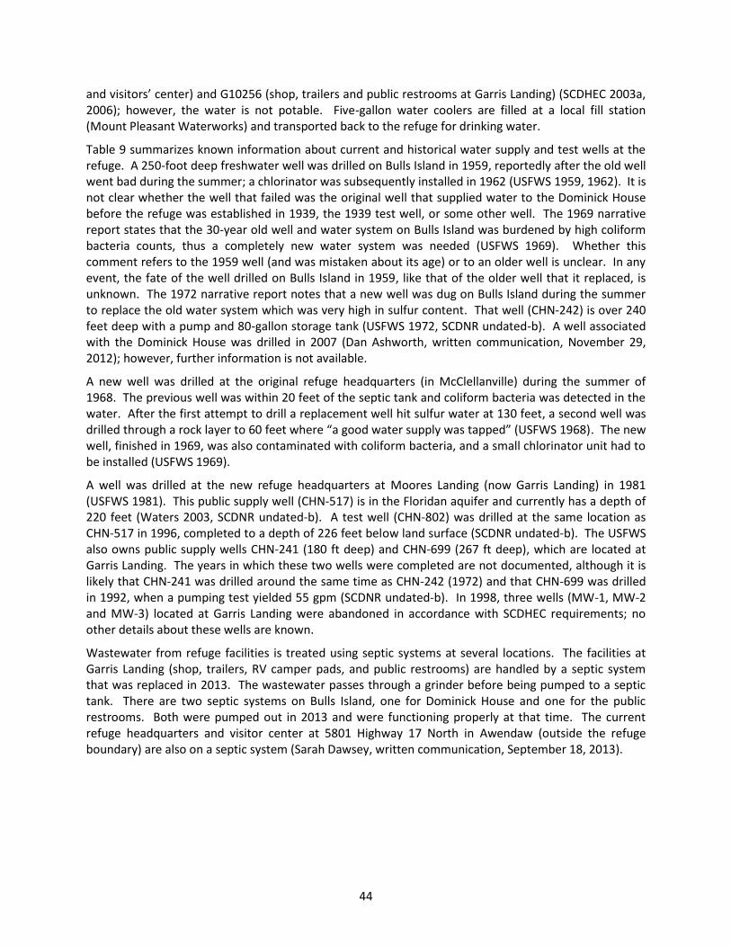
44

and visitors’ center) and G10256 (shop, trailers and public restrooms at Garris Landing) (SCDHEC 2003a, 2006); however, the water is not potable. Five-gallon water coolers are filled at a local fill station (Mount Pleasant Waterworks) and transported back to the refuge for drinking water.

Table 9 summarizes known information about current and historical water supply and test wells at the refuge. A 250-foot deep freshwater well was drilled on Bulls Island in 1959, reportedly after the old well went bad during the summer; a chlorinator was subsequently installed in 1962 (USFWS 1959, 1962). It is not clear whether the well that failed was the original well that supplied water to the Dominick House before the refuge was established in 1939, the 1939 test well, or some other well. The 1969 narrative report states that the 30-year old well and water system on Bulls Island was burdened by high coliform bacteria counts, thus a completely new water system was needed (USFWS 1969). Whether this comment refers to the 1959 well (and was mistaken about its age) or to an older well is unclear. In any event, the fate of the well drilled on Bulls Island in 1959, like that of the older well that it replaced, is unknown. The 1972 narrative report notes that a new well was dug on Bulls Island during the summer to replace the old water system which was very high in sulfur content. That well (CHN-242) is over 240 feet deep with a pump and 80-gallon storage tank (USFWS 1972, SCDNR undated-b). A well associated with the Dominick House was drilled in 2007 (Dan Ashworth, written communication, November 29, 2012); however, further information is not available.

A new well was drilled at the original refuge headquarters (in McClellanville) during the summer of 1968. The previous well was within 20 feet of the septic tank and coliform bacteria was detected in the water. After the first attempt to drill a replacement well hit sulfur water at 130 feet, a second well was drilled through a rock layer to 60 feet where “a good water supply was tapped” (USFWS 1968). The new well, finished in 1969, was also contaminated with coliform bacteria, and a small chlorinator unit had to be installed (USFWS 1969).

A well was drilled at the new refuge headquarters at Moores Landing (now Garris Landing) in 1981 (USFWS 1981). This public supply well (CHN-517) is in the Floridan aquifer and currently has a depth of 220 feet (Waters 2003, SCDNR undated-b). A test well (CHN-802) was drilled at the same location as CHN-517 in 1996, completed to a depth of 226 feet below land surface (SCDNR undated-b). The USFWS also owns public supply wells CHN-241 (180 ft deep) and CHN-699 (267 ft deep), which are located at Garris Landing. The years in which these two wells were completed are not documented, although it is likely that CHN-241 was drilled around the same time as CHN-242 (1972) and that CHN-699 was drilled in 1992, when a pumping test yielded 55 gpm (SCDNR undated-b). In 1998, three wells (MW-1, MW-2 and MW-3) located at Garris Landing were abandoned in accordance with SCDHEC requirements; no other details about these wells are known.

Wastewater from refuge facilities is treated using septic systems at several locations. The facilities at Garris Landing (shop, trailers, RV camper pads, and public restrooms) are handled by a septic system that was replaced in 2013. The wastewater passes through a grinder before being pumped to a septic tank. There are two septic systems on Bulls Island, one for Dominick House and one for the public restrooms. Both were pumped out in 2013 and were functioning properly at that time. The current refuge headquarters and visitor center at 5801 Highway 17 North in Awendaw (outside the refuge boundary) are also on a septic system (Sarah Dawsey, written communication, September 18, 2013).

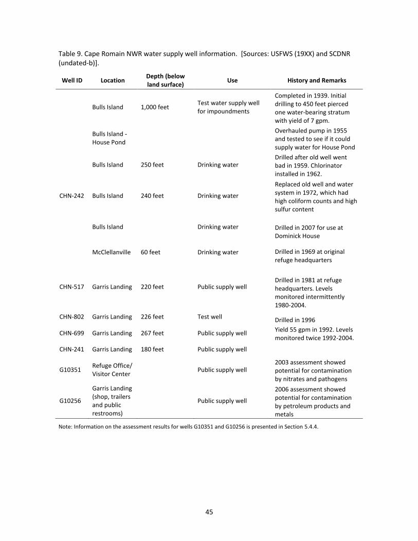
45

Table 9. Cape Romain NWR water supply well information. [Sources: USFWS (19XX) and SCDNR (undated-b)].

Well ID Location Depth (below land surface)

Use History and Remarks

Bulls Island 1,000 feet

Test water supply well for impoundments

Completed in 1939. Initial drilling to 450 feet pierced one water-bearing stratum with yield of 7 gpm.

Bulls Island - House Pond

Overhauled pump in 1955 and tested to see if it could supply water for House Pond

Bulls Island 250 feet Drinking water

Drilled after old well went bad in 1959. Chlorinator installed in 1962.

CHN-242 Bulls Island 240 feet Drinking water

Replaced old well and water system in 1972, which had high coliform counts and high sulfur content

Bulls Island

Drinking water Drilled in 2007 for use at

Dominick House

McClellanville 60 feet Drinking water Drilled in 1969 at original

refuge headquarters

CHN-517 Garris Landing 220 feet Public supply well Drilled in 1981 at refuge headquarters. Levels monitored intermittently 1980-2004.

CHN-802 Garris Landing 226 feet Test well Drilled in 1996

CHN-699 Garris Landing 267 feet Public supply well Yield 55 gpm in 1992. Levels monitored twice 1992-2004.

CHN-241 Garris Landing 180 feet Public supply well

G10351 Refuge Office/ Visitor Center

Public supply well 2003 assessment showed potential for contamination by nitrates and pathogens

G10256

Garris Landing (shop, trailers and public restrooms)

Public supply well

2006 assessment showed potential for contamination by petroleum products and metals

Note: Information on the assessment results for wells G10351 and G10256 is presented in Section 5.4.4.

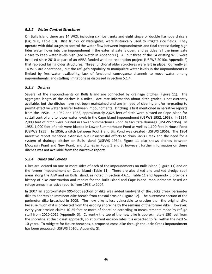
46

5.2.2 Water Control Structures

On Bulls Island there are 14 WCS, including six rice trunks and eight single or double flashboard risers (Figure 8, Table 10). Rice trunks, or watergates, were historically used to irrigate rice fields. They operate with tidal surges to control the water flow between impoundments and tidal creeks; during high tides water flows into the impoundment if the external gate is open, and as tides fall the inner gate closes to keep water levels high (see sketch in Appendix F). All but three of the 14 existing WCS were installed since 2010 as part of an ARRA-funded wetland restoration project (USFWS 2010c, Appendix F) that replaced failing older structures. Three functional older structures were left in place. Currently all 14 WCS are operational, but the refuge’s capability to manipulate water levels in the impoundments is limited by freshwater availability, lack of functional conveyance channels to move water among impoundments, and staffing limitations as discussed in Section 5.1.4.

5.2.3 Ditches

Several of the impoundments on Bulls Island are connected by drainage ditches (Figure 11). The aggregate length of the ditches is 4 miles. Accurate information about ditch grades is not currently available, but the ditches have not been maintained and are in need of clearing and/or re-grading to permit effective water transfer between impoundments. Ditching is first mentioned in narrative reports from the 1950s. In 1952 and 1953, approximately 2,625 feet of ditch were blasted on Cape Island for cattail control and to lower water levels in the Cape Island impoundment (USFWS 1952, 1953). In 1954, 2,000 feet of ditch were blasted in Lower Summerhouse Pond to facilitate drainage (USFWS 1954). In 1955, 1,000 feet of ditch were blasted in Lower Summerhouse Pond as well as 1,100 feet in House Pond (USFWS 1955). In 1956, a ditch between Pool 2 and Big Pond was created (USFWS 1956). The 1964 narrative report mentions extensive but unsuccessful efforts to drain Jacks Creek and the need for a system of drainage ditches on Bulls Island (USFWS 1964). Figure 11 also shows ditches between Moccasin Pond and New Pond, and ditches in Pools 1 and 3; however, further information on these ditches was not available from the narrative reports.

5.2.4 Dikes and Levees

Dikes are located on one or more sides of each of the impoundments on Bulls Island (Figure 11) and on the former impoundment on Cape Island (Table 11). There are also diked and undiked dredge spoil areas along the AIW and on Bulls Island, as noted in Section 4.6.1. Table 11 and Appendix E provide a history of dike construction and repairs for the Bulls Island and Cape Island impoundments based on refuge annual narrative reports from 1938 to 2004.

In 2007 an approximately 995-foot section of dike was added landward of the Jacks Creek perimeter dike to address an imminent dike breach from coastal erosion (Figure 12). The outermost section of the perimeter dike breached in 2009. The new dike is less vulnerable to erosion than the original dike because much of it is protected from the eroding shoreline by the remains of the former dike. However, every year erosion claims 10-25 feet or more of shoreline according to measurements made by refuge staff from 2010-2012 (Appendix D). Currently the toe of the new dike is approximately 150 feet from the shoreline at the closest approach, so at current erosion rates it is expected to fail within the next 5-10 years. To mitigate for future breaches, a proposed cross-dike through the Jacks Creek impoundment has been proposed (USFWS 2010b, Appendix G).

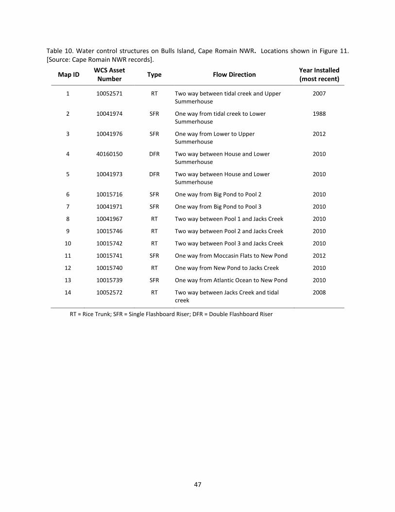
47

Table 10. Water control structures on Bulls Island, Cape Romain NWR. Locations shown in Figure 11. [Source: Cape Romain NWR records].

Map ID WCS Asset

Number Type Flow Direction

Year Installed (most recent)

1 10052571 RT Two way between tidal creek and Upper Summerhouse

2007

2 10041974 SFR One way from tidal creek to Lower Summerhouse

1988

3 10041976 SFR One way from Lower to Upper Summerhouse

2012

4 40160150 DFR Two way between House and Lower Summerhouse

2010

5 10041973 DFR Two way between House and Lower Summerhouse

2010

6 10015716 SFR One way from Big Pond to Pool 2 2010

7 10041971 SFR One way from Big Pond to Pool 3 2010

8 10041967 RT Two way between Pool 1 and Jacks Creek 2010



11 10015741 SFR One way from Moccasin Flats to New Pond 2012

12 10015740 RT One way from New Pond to Jacks Creek 2010

13 10015739 SFR One way from Atlantic Ocean to New Pond 2010

14 10052572 RT Two way between Jacks Creek and tidal creek

2008

RT = Rice Trunk; SFR = Single Flashboard Riser; DFR = Double Flashboard Riser

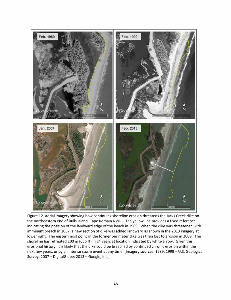
48

Figure 12. Aerial imagery showing how continuing shoreline erosion threatens the Jacks Creek dike on the northeastern end of Bulls Island, Cape Romain NWR. The yellow line provides a fixed reference indicating the position of the landward edge of the beach in 1989. When the dike was threatened with imminent breach in 2007, a new section of dike was added landward as shown in the 2013 imagery at lower right. The easternmost point of the former perimeter dike was then lost to erosion in 2009. The shoreline has retreated 200 m (656 ft) in 24 years at location indicated by white arrow. Given this erosional history, it is likely that the dike could be breached by continued chronic erosion within the next few years, or by an intense storm event at any time. [Imagery sources: 1989, 1999 – U.S. Geological Survey; 2007 – DigitalGlobe; 2013 – Google, Inc.]

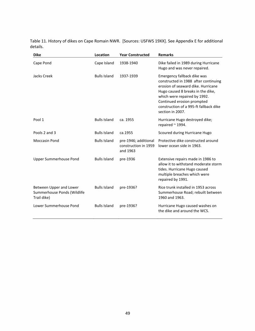
49

Table 11. History of dikes on Cape Romain NWR. [Sources: USFWS 19XX]. See Appendix E for additional details.

Dike Location Year Constructed Remarks

Cape Pond Cape Island 1938-1940 Dike failed in 1989 during Hurricane Hugo and was never repaired.

Jacks Creek Bulls Island 1937-1939 Emergency fallback dike was constructed in 1988 after continuing erosion of seaward dike. Hurricane Hugo caused 8 breaks in the dike, which were repaired by 1992. Continued erosion prompted construction of a 995-ft fallback dike section in 2007.

Pool 1 Bulls Island ca. 1955 Hurricane Hugo destroyed dike; repaired ~ 1994.

Pools 2 and 3 Bulls Island ca.1955 Scoured during Hurricane Hugo

Moccasin Pond Bulls Island pre-1946; additional construction in 1959 and 1963

Protective dike constructed around lower ocean side in 1963.

Upper Summerhouse Pond Bulls Island pre-1936 Extensive repairs made in 1986 to allow it to withstand moderate storm tides. Hurricane Hugo caused multiple breaches which were repaired by 1991.

Between Upper and Lower Summerhouse Ponds (Wildlife Trail dike)

Bulls Island pre-1936? Rice trunk installed in 1953 across Summerhouse Road; rebuilt between 1960 and 1963.

Lower Summerhouse Pond Bulls Island pre-1936? Hurricane Hugo caused washes on the dike and around the WCS.

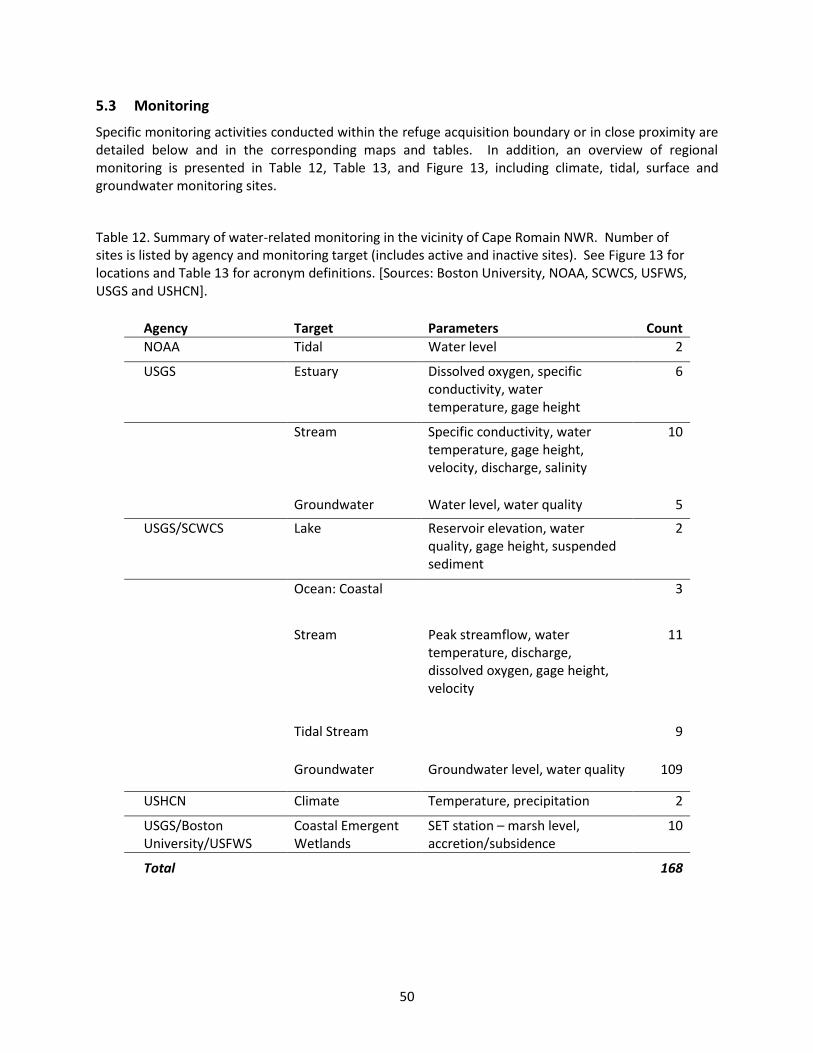
50

5.3 Monitoring

Specific monitoring activities conducted within the refuge acquisition boundary or in close proximity are detailed below and in the corresponding maps and tables. In addition, an overview of regional monitoring is presented in Table 12, Table 13, and Figure 13, including climate, tidal, surface and groundwater monitoring sites.

Table 12. Summary of water-related monitoring in the vicinity of Cape Romain NWR. Number of sites is listed by agency and monitoring target (includes active and inactive sites). See Figure 13 for locations and Table 13 for acronym definitions. [Sources: Boston University, NOAA, SCWCS, USFWS, USGS and USHCN].

Agency Target Parameters Count

NOAA Tidal Water level 2

USGS Estuary Dissolved oxygen, specific conductivity, water temperature, gage height

6

Stream Specific conductivity, water temperature, gage height, velocity, discharge, salinity

10

Groundwater Water level, water quality 5

USGS/SCWCS Lake Reservoir elevation, water quality, gage height, suspended sediment

2

Ocean: Coastal 3

Stream Peak streamflow, water temperature, discharge, dissolved oxygen, gage height, velocity

11

Tidal Stream 9

Groundwater Groundwater level, water quality 109

USHCN Climate Temperature, precipitation 2

USGS/Boston University/USFWS

Coastal Emergent Wetlands

SET station – marsh level, accretion/subsidence

10

Total

168

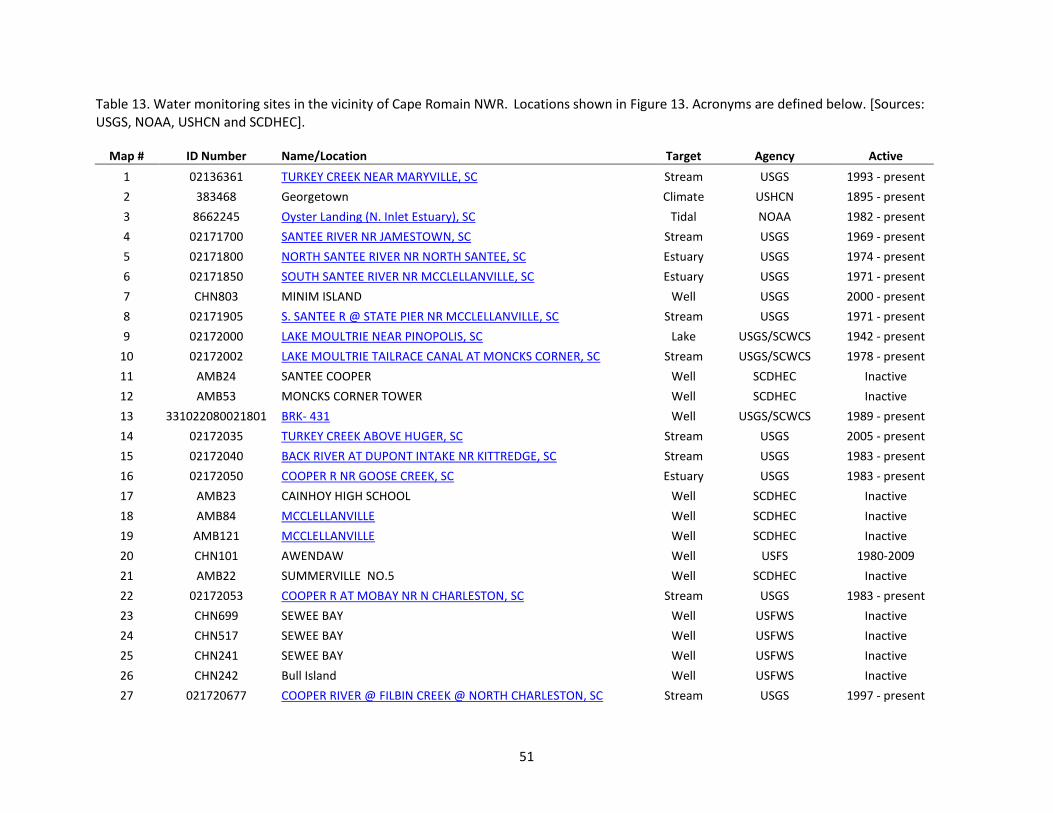
51

Table 13. Water monitoring sites in the vicinity of Cape Romain NWR. Locations shown in Figure 13. Acronyms are defined below. [Sources: USGS, NOAA, USHCN and SCDHEC].

Map # ID Number Name/Location Target Agency Active

1 02136361 TURKEY CREEK NEAR MARYVILLE, SC Stream USGS 1993 - present

2 383468 Georgetown Climate USHCN 1895 - present

3 8662245 Oyster Landing (N. Inlet Estuary), SC Tidal NOAA 1982 - present

4 02171700 SANTEE RIVER NR JAMESTOWN, SC Stream USGS 1969 - present

5 02171800 NORTH SANTEE RIVER NR NORTH SANTEE, SC Estuary USGS 1974 - present

6 02171850 SOUTH SANTEE RIVER NR MCCLELLANVILLE, SC Estuary USGS 1971 - present

7 CHN803 MINIM ISLAND Well USGS 2000 - present

8 02171905 S. SANTEE R @ STATE PIER NR MCCLELLANVILLE, SC Stream USGS 1971 - present

9 02172000 LAKE MOULTRIE NEAR PINOPOLIS, SC Lake USGS/SCWCS 1942 - present

10 02172002 LAKE MOULTRIE TAILRACE CANAL AT MONCKS CORNER, SC Stream USGS/SCWCS 1978 - present

11 AMB24 SANTEE COOPER Well SCDHEC Inactive

12 AMB53 MONCKS CORNER TOWER Well SCDHEC Inactive

13 331022080021801 BRK- 431 Well USGS/SCWCS 1989 - present

14 02172035 TURKEY CREEK ABOVE HUGER, SC Stream USGS 2005 - present

15 02172040 BACK RIVER AT DUPONT INTAKE NR KITTREDGE, SC Stream USGS 1983 - present

16 02172050 COOPER R NR GOOSE CREEK, SC Estuary USGS 1983 - present

17 AMB23 CAINHOY HIGH SCHOOL Well SCDHEC Inactive

18 AMB84 MCCLELLANVILLE Well SCDHEC Inactive

19 AMB121 MCCLELLANVILLE Well SCDHEC Inactive

20 CHN101 AWENDAW Well USFS 1980-2009

21 AMB22 SUMMERVILLE NO.5 Well SCDHEC Inactive

22 02172053 COOPER R AT MOBAY NR N CHARLESTON, SC Stream USGS 1983 - present

23 CHN699 SEWEE BAY Well USFWS Inactive



26 CHN242 Bull Island Well USFWS Inactive

27 021720677 COOPER RIVER @ FILBIN CREEK @ NORTH CHARLESTON, SC Stream USGS 1997 - present

http://waterdata.usgs.gov/nwis/inventory?agency_code=USGS&site_no=02136361&target=_

http://tidesandcurrents.noaa.gov/geo.shtml?location=8662245











http://www.scdhec.gov/environment/water/docs/amb2002.pdf




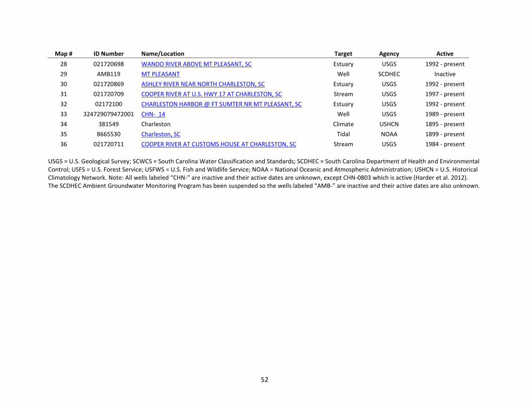
52

Map # ID Number Name/Location Target Agency Active

28 021720698 WANDO RIVER ABOVE MT PLEASANT, SC Estuary USGS 1992 - present

29 AMB119 MT PLEASANT Well SCDHEC Inactive

30 021720869 ASHLEY RIVER NEAR NORTH CHARLESTON, SC Estuary USGS 1992 - present

31 021720709 COOPER RIVER AT U.S. HWY 17 AT CHARLESTON, SC Stream USGS 1997 - present

32 02172100 CHARLESTON HARBOR @ FT SUMTER NR MT PLEASANT, SC Estuary USGS 1992 - present

33 324729079472001 CHN- 14 Well USGS 1989 - present

34 381549 Charleston Climate USHCN 1895 - present

35 8665530 Charleston, SC Tidal NOAA 1899 - present

36 021720711 COOPER RIVER AT CUSTOMS HOUSE AT CHARLESTON, SC Stream USGS 1984 - present

USGS = U.S. Geological Survey; SCWCS = South Carolina Water Classification and Standards; SCDHEC = South Carolina Department of Health and Environmental Control; USFS = U.S. Forest Service; USFWS = U.S. Fish and Wildlife Service; NOAA = National Oceanic and Atmospheric Administration; USHCN = U.S. Historical Climatology Network. Note: All wells labeled “CHN-” are inactive and their active dates are unknown, except CHN-0803 which is active (Harder et al. 2012). The SCDHEC Ambient Groundwater Monitoring Program has been suspended so the wells labeled “AMB-” are inactive and their active dates are also unknown.







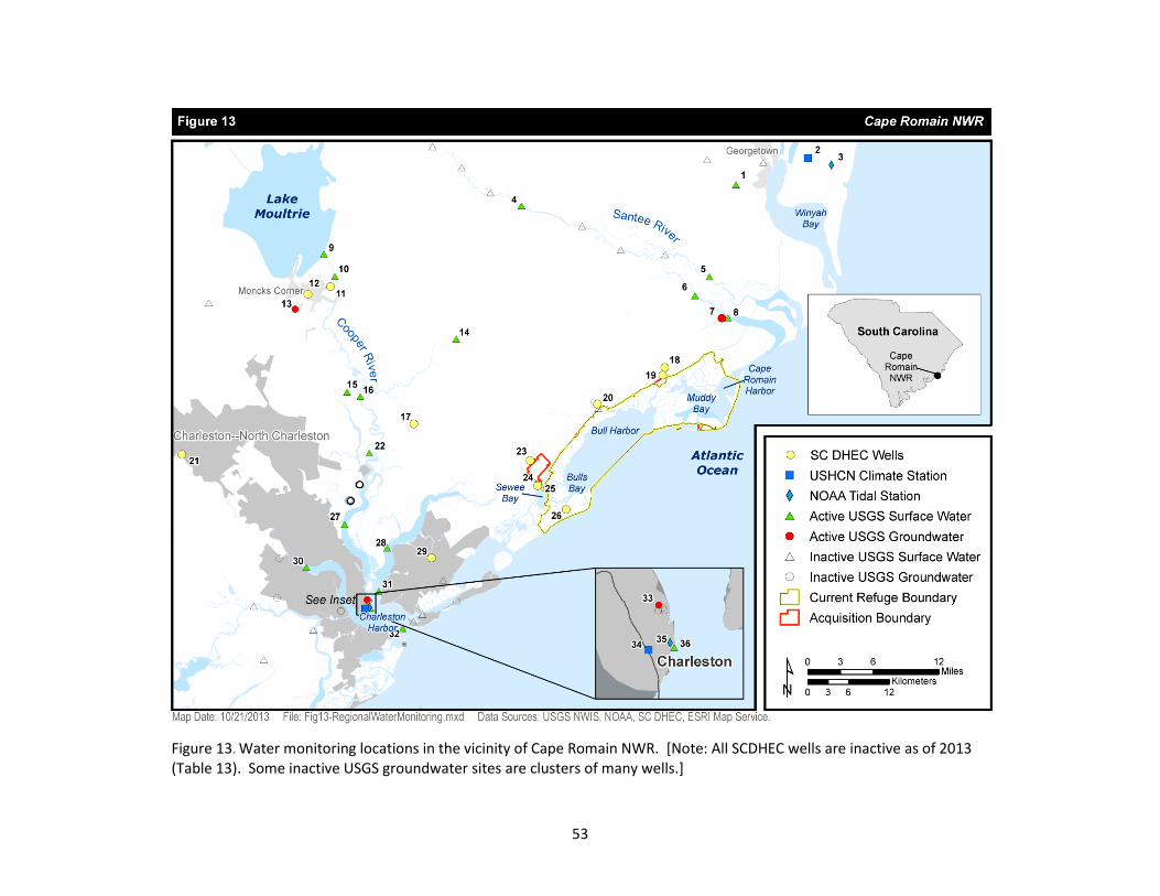
http://tidesandcurrents.noaa.gov/geo.shtml?location=8665530


53

Figure 13. Water monitoring locations in the vicinity of Cape Romain NWR. [Note: All SCDHEC wells are inactive as of 2013 (Table 13). Some inactive USGS groundwater sites are clusters of many wells.]

54

5.3.1 Surface Water

5.3.1.1 Precipitation, streamflow, and water levels

The refuge has monitored precipitation at Garris Landing since 2000 as part of its participation in the National Atmospheric Deposition Program (NADP undated). In addition, the refuge monitors precipitation on Bulls Island year-round (daily from May through September and weekly the rest of the year; Table 1) and on Cape Island during the sea turtle field season (May through September). Precipitation is also monitored at the two USHCN sites in Charleston and Georgetown (Section 4.2.1). Streamflow is measured at a total of 21 sites in the refuge vicinity, primarily on the Cooper and Santee rivers. In addition, the USGS conducts estuarine monitoring at six sites (Table 12, Table 13, Figure 13.)

Impoundment water level monitoring was first reported in the 1942 narrative report; readings were taken three times during each quarter of the year (USFWS 1942). Beginning in 1944, more frequent water level readings were taken (i.e., at least once per month). Desired water level ranges were established for December – February, March – May, June – August and September – November (e.g., USFWS 1966). The 1984 Water Management Plan included desired water level ranges for each impoundment and stated that no impoundment should exceed 7 feet (USFWS 1984). Impoundment water levels continue to be monitored and adjusted as necessary and feasible, given management constraints.

5.3.1.2 Tidal monitoring

The nearest NOAA tide gages to the refuge are Station 8665530, located at Charleston, SC, and Station 8662245, located at Oyster Landing (N. Inlet Estuary) near Georgetown, SC. The Charleston station was first established in 1899, with the present installation occurring in 1990, while the Georgetown station was first established in 1982 with the present installation in 2001. Tide gages record a local measurement of sea level relative to a fixed point on land near the gage site. Mean tidal range is 5.22 feet (1.57 m) at the Charleston gage and 4.58 feet (1.40 m) at the Georgetown gage, whereas diurnal ranges are 5.77 feet (1.76 m) and 5.12 feet (1.56 m), respectively. The estimated mean sea level difference between sampling periods of 1960-1978 and 1983-2001 at the Charleston site is 0.25 feet (7.6 cm) and 0.34 feet (10.4 cm) at Georgetown (NOAA undated).

As discussed in Section 4.7.2, long-term sea level trends available from the Charleston tide gage suggest the local sea level is rising about 3.10 millimeters (0.12 inches) per year, based on mean monthly sea level data from 1921 to 2006. Tidal monitoring at the Charleston gage also reveals seasonal variations in mean sea level due to the combined effects of seasonal variations in temperature, salinity, winds, atmospheric pressure, and ocean currents. Monthly mean sea level is at its lowest from January through March (-0.09 to -0.07 m) and at its highest in September and October (+0.12 to 0.15 m), an annual range of 0.24 m (0.8 ft) (Figure 14). It is worth noting that mean sea level at Charleston is at its highest during the peak of tropical cyclone season, which runs from June through November.

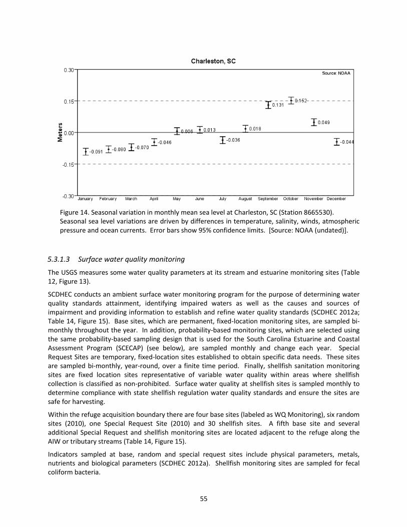
55

Figure 14. Seasonal variation in monthly mean sea level at Charleston, SC (Station 8665530). Seasonal sea level variations are driven by differences in temperature, salinity, winds, atmospheric pressure and ocean currents. Error bars show 95% confidence limits. [Source: NOAA (undated)].

5.3.1.3 Surface water quality monitoring

The USGS measures some water quality parameters at its stream and estuarine monitoring sites (Table 12, Figure 13).

SCDHEC conducts an ambient surface water monitoring program for the purpose of determining water quality standards attainment, identifying impaired waters as well as the causes and sources of impairment and providing information to establish and refine water quality standards (SCDHEC 2012a; Table 14, Figure 15). Base sites, which are permanent, fixed-location monitoring sites, are sampled bi-monthly throughout the year. In addition, probability-based monitoring sites, which are selected using the same probability-based sampling design that is used for the South Carolina Estuarine and Coastal Assessment Program (SCECAP) (see below), are sampled monthly and change each year. Special Request Sites are temporary, fixed-location sites established to obtain specific data needs. These sites are sampled bi-monthly, year-round, over a finite time period. Finally, shellfish sanitation monitoring sites are fixed location sites representative of variable water quality within areas where shellfish collection is classified as non-prohibited. Surface water quality at shellfish sites is sampled monthly to determine compliance with state shellfish regulation water quality standards and ensure the sites are safe for harvesting.

Within the refuge acquisition boundary there are four base sites (labeled as WQ Monitoring), six random sites (2010), one Special Request Site (2010) and 30 shellfish sites. A fifth base site and several additional Special Request and shellfish monitoring sites are located adjacent to the refuge along the AIW or tributary streams (Table 14, Figure 15).

Indicators sampled at base, random and special request sites include physical parameters, metals, nutrients and biological parameters (SCDHEC 2012a). Shellfish monitoring sites are sampled for fecal coliform bacteria.

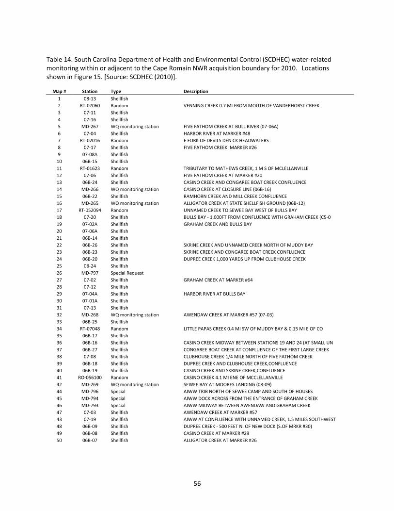
56

Table 14. South Carolina Department of Health and Environmental Control (SCDHEC) water-related monitoring within or adjacent to the Cape Romain NWR acquisition boundary for 2010. Locations shown in Figure 15. [Source: SCDHEC (2010)].

Map # Station Type Description

1 08-13 Shellfish

2 RT-07060 Random VENNING CREEK 0.7 MI FROM MOUTH OF VANDERHORST CREEK

3 07-11 Shellfish

4 07-16 Shellfish

5 MD-267 WQ monitoring station FIVE FATHOM CREEK AT BULL RIVER (07-06A)

6 07-04 Shellfish HARBOR RIVER AT MARKER #48

7 RT-02016 Random E FORK OF DEVILS DEN CK HEADWATERS

8 07-17 Shellfish FIVE FATHOM CREEK MARKER #26

9 07-08A Shellfish

10 06B-15 Shellfish

11 RT-01623 Random TRIBUTARY TO MATHEWS CREEK, 1 M S OF MCLELLANVILLE

12 07-06 Shellfish FIVE FATHOM CREEK AT MARKER #20

13 06B-24 Shellfish CASINO CREEK AND CONGAREE BOAT CREEK CONFLUENCE

14 MD-266 WQ monitoring station CASINO CREEK AT CLOSURE LINE (06B-16)

15 06B-22 Shellfish RAMHORN CREEK AND MILL CREEK CONFLUENCE

16 MD-265 WQ monitoring station ALLIGATOR CREEK AT STATE SHELLFISH GROUND (06B-12)

17 RT-052094 Random UNNAMED CREEK TO SEWEE BAY WEST OF BULLS BAY

18 07-20 Shellfish BULLS BAY - 1,000FT FROM CONFLUENCE WITH GRAHAM CREEK (C5-0

19 07-02A Shellfish GRAHAM CREEK AND BULLS BAY

20 07-06A Shellfish

21 06B-14 Shellfish

22 06B-26 Shellfish SKRINE CREEK AND UNNAMED CREEK NORTH OF MUDDY BAY

23 06B-23 Shellfish SKRINE CREEK AND CONGAREE BOAT CREEK CONFLUENCE

24 06B-20 Shellfish DUPREE CREEK 1,000 YARDS UP FROM CLUBHOUSE CREEK

25 08-24 Shellfish

26 MD-797 Special Request

27 07-02 Shellfish GRAHAM CREEK AT MARKER #64

28 07-12 Shellfish

29 07-04A Shellfish HARBOR RIVER AT BULLS BAY

30 07-01A Shellfish

31 07-13 Shellfish

32 MD-268 WQ monitoring station AWENDAW CREEK AT MARKER #57 (07-03)

33 06B-25 Shellfish

34 RT-07048 Random LITTLE PAPAS CREEK 0.4 MI SW OF MUDDY BAY & 0.15 MI E OF CO

35 06B-17 Shellfish

36 06B-16 Shellfish CASINO CREEK MIDWAY BETWEEN STATIONS 19 AND 24 (AT SMALL UN

37 06B-27 Shellfish CONGAREE BOAT CREEK AT CONFLUENCE OF THE FIRST LARGE CREEK

38 07-08 Shellfish CLUBHOUSE CREEK-1/4 MILE NORTH OF FIVE FATHOM CREEK

39 06B-18 Shellfish DUPREE CREEK AND CLUBHOUSE CREEK,CONFLUENCE

40 06B-19 Shellfish CASINO CREEK AND SKRINE CREEK,CONFLUENCE

41 RO-056100 Random CASINO CREEK 4.1 MI ENE OF MCCLELLANVILLE

42 MD-269 WQ monitoring station SEWEE BAY AT MOORES LANDING (08-09)

44 MD-796 Special AIWW TRIB NORTH OF SEWEE CAMP AND SOUTH OF HOUSES

45 MD-794 Special AIWW DOCK ACROSS FROM THE ENTRANCE OF GRAHAM CREEK

46 MD-793 Special AIWW MIDWAY BETWEEN AWENDAW AND GRAHAM CREEK

47 07-03 Shellfish AWENDAW CREEK AT MARKER #57

43 07-19 Shellfish AIWW AT CONFLUENCE WITH UNNAMED CREEK, 1.5 MILES SOUTHWEST

48 06B-09 Shellfish DUPREE CREEK - 500 FEET N. OF NEW DOCK (S.OF MRKR #30)

49 06B-08 Shellfish CASINO CREEK AT MARKER #29

50 06B-07 Shellfish ALLIGATOR CREEK AT MARKER #26

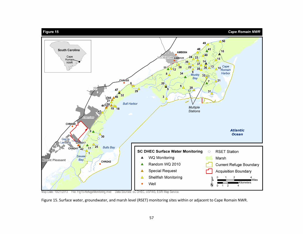
57

Figure 15. Surface water, groundwater, and marsh level (RSET) monitoring sites within or adjacent to Cape Romain NWR.

58

The SCECAP is a multi-agency coastal monitoring program that measures surface water quality, sediment quality and biological condition and integrates the results into an overall assessment of estuarine habitat condition. The program began in 1999 and the latest biennial report assesses 2007-2008 data (Bergquist et al. 2011). The SCECAP program, implemented by the SCDNR and SCDHEC since 1999, samples surface water quality at coastal sites (both tidal creeks and open water) located throughout South Carolina on an annual basis (Table 15, Figure 16). Stations are selected by SCDNR and SCDHEC using a shared probability-based sampling design and change each year. Samples are collected using YSI probes to measure physical parameters (temperature, DO, pH, salinity) as well as grab samples, which are analyzed for total nutrients, total organic carbon (TOC), total alkalinity, total suspended solids (TSS), turbidity, biological oxygen demand (BOD), fecal coliform bacteria and chlorophyll-a (Chl-a). Six surface water quality parameters are combined to obtain a Water Quality Score for each site: fecal coliform bacteria, DO, pH, total nitrogen (TN), total phosphorus (TP) and Chl-a. Similarly, three sediment quality measures (contaminants, toxicity, and TOC) are combined into a Sediment Quality Index, and benthic invertebrate sampling data are used to compute a benthic index of biotic integrity (B-IBI). These three indices are then combined into an overall Habitat Quality Index (Berquist et al. 2011).

Beginning in 1942, salinity measurements were taken in specific points in Jacks Creek and Cape Island Pond impoundments. The method used was silver nitrate titration and results were reported in percentages of sea strength (PSS) (USFWS 1942). The number of sampling sites and frequency increased over the years. The 1984 Water Management Plan states that salinity readings were taken monthly at a set location in eight impoundments. Target salinity ranges were established for each location: 1-5 PSS at Big Pond, 1-10 PSS at Moccasin Pond, Pool 2, Pool 3, House Pond and Lower Summerhouse Pond, and 10-20 PSS at Jacks Creek and Upper Summerhouse ponds. Salinity manipulation was possible in at least the two exterior ponds (USFWS 1984); salinity levels were manipulated to control cattail growth (e.g., USFWS 1987). Currently salinity is monitored at 13 sites (Figure 17) at least monthly; additional parameters (temperature, pH, and conductivity) were also monitored at these locations between December 2011 and June 2012 (Appendix H).

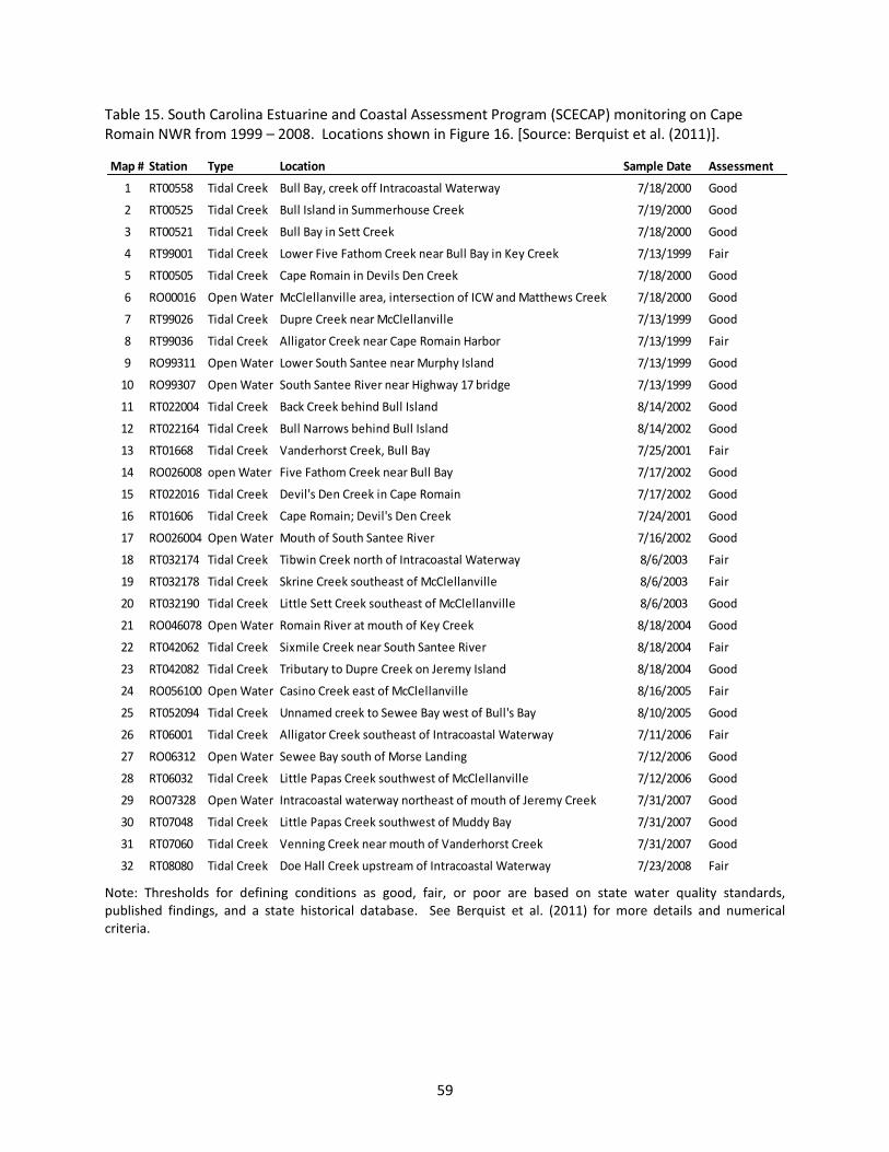
59

Table 15. South Carolina Estuarine and Coastal Assessment Program (SCECAP) monitoring on Cape Romain NWR from 1999 – 2008. Locations shown in Figure 16. [Source: Berquist et al. (2011)].

Note: Thresholds for defining conditions as good, fair, or poor are based on state water quality standards, published findings, and a state historical database. See Berquist et al. (2011) for more details and numerical criteria.

Map # Station Type Location Sample Date Assessment

1 RT00558 Tidal Creek Bull Bay, creek off Intracoastal Waterway 7/18/2000 Good

2 RT00525 Tidal Creek Bull Island in Summerhouse Creek 7/19/2000 Good

3 RT00521 Tidal Creek Bull Bay in Sett Creek 7/18/2000 Good

4 RT99001 Tidal Creek Lower Five Fathom Creek near Bull Bay in Key Creek 7/13/1999 Fair

5 RT00505 Tidal Creek Cape Romain in Devils Den Creek 7/18/2000 Good

6 RO00016 Open Water McClellanville area, intersection of ICW and Matthews Creek 7/18/2000 Good

7 RT99026 Tidal Creek Dupre Creek near McClellanville 7/13/1999 Good

8 RT99036 Tidal Creek Alligator Creek near Cape Romain Harbor 7/13/1999 Fair

9 RO99311 Open Water Lower South Santee near Murphy Island 7/13/1999 Good

10 RO99307 Open Water South Santee River near Highway 17 bridge 7/13/1999 Good

11 RT022004 Tidal Creek Back Creek behind Bull Island 8/14/2002 Good

12 RT022164 Tidal Creek Bull Narrows behind Bull Island 8/14/2002 Good

13 RT01668 Tidal Creek Vanderhorst Creek, Bull Bay 7/25/2001 Fair

14 RO026008 open Water Five Fathom Creek near Bull Bay 7/17/2002 Good

15 RT022016 Tidal Creek Devil's Den Creek in Cape Romain 7/17/2002 Good

16 RT01606 Tidal Creek Cape Romain; Devil's Den Creek 7/24/2001 Good

17 RO026004 Open Water Mouth of South Santee River 7/16/2002 Good

18 RT032174 Tidal Creek Tibwin Creek north of Intracoastal Waterway 8/6/2003 Fair

19 RT032178 Tidal Creek Skrine Creek southeast of McClellanville 8/6/2003 Fair

20 RT032190 Tidal Creek Little Sett Creek southeast of McClellanville 8/6/2003 Good

21 RO046078 Open Water Romain River at mouth of Key Creek 8/18/2004 Good

22 RT042062 Tidal Creek Sixmile Creek near South Santee River 8/18/2004 Fair

23 RT042082 Tidal Creek Tributary to Dupre Creek on Jeremy Island 8/18/2004 Good

24 RO056100 Open Water Casino Creek east of McClellanville 8/16/2005 Fair

25 RT052094 Tidal Creek Unnamed creek to Sewee Bay west of Bull's Bay 8/10/2005 Good

26 RT06001 Tidal Creek Alligator Creek southeast of Intracoastal Waterway 7/11/2006 Fair

27 RO06312 Open Water Sewee Bay south of Morse Landing 7/12/2006 Good

28 RT06032 Tidal Creek Little Papas Creek southwest of McClellanville 7/12/2006 Good

29 RO07328 Open Water Intracoastal waterway northeast of mouth of Jeremy Creek 7/31/2007 Good

30 RT07048 Tidal Creek Little Papas Creek southwest of Muddy Bay 7/31/2007 Good

31 RT07060 Tidal Creek Venning Creek near mouth of Vanderhorst Creek 7/31/2007 Good

32 RT08080 Tidal Creek Doe Hall Creek upstream of Intracoastal Waterway 7/23/2008 Fair

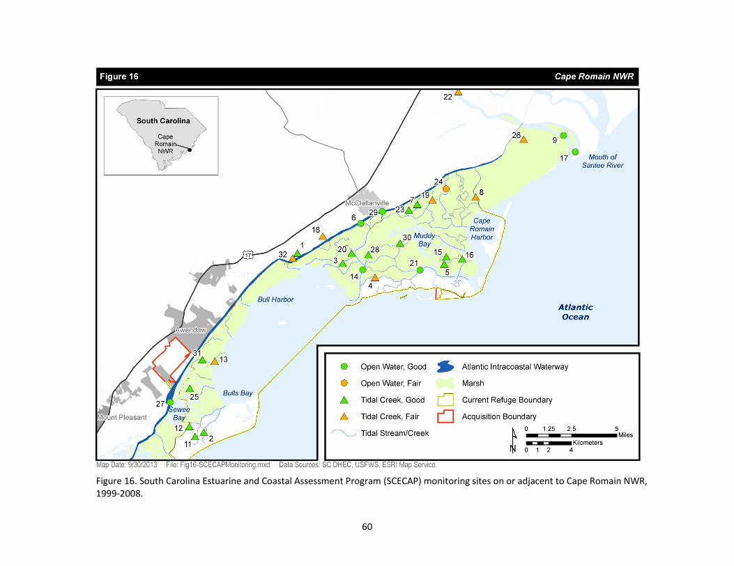
60

Figure 16. South Carolina Estuarine and Coastal Assessment Program (SCECAP) monitoring sites on or adjacent to Cape Romain NWR, 1999-2008.

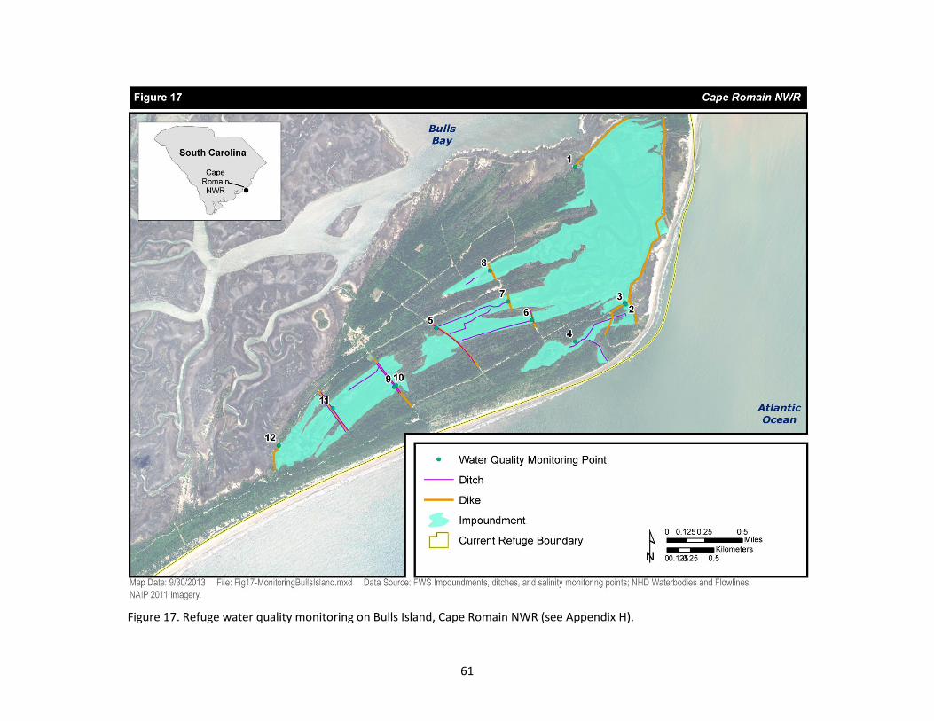
61

Figure 17. Refuge water quality monitoring on Bulls Island, Cape Romain NWR (see Appendix H).

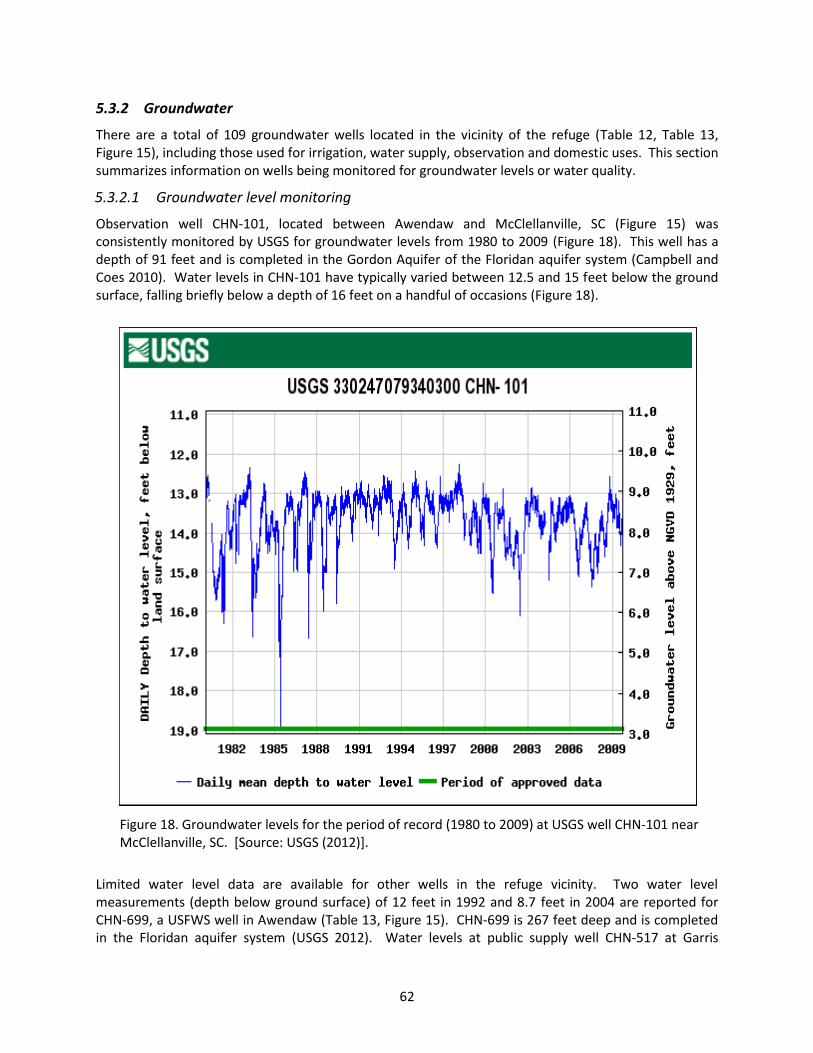
62

5.3.2 Groundwater

There are a total of 109 groundwater wells located in the vicinity of the refuge (Table 12, Table 13, Figure 15), including those used for irrigation, water supply, observation and domestic uses. This section summarizes information on wells being monitored for groundwater levels or water quality.

5.3.2.1 Groundwater level monitoring

Observation well CHN-101, located between Awendaw and McClellanville, SC (Figure 15) was consistently monitored by USGS for groundwater levels from 1980 to 2009 (Figure 18). This well has a depth of 91 feet and is completed in the Gordon Aquifer of the Floridan aquifer system (Campbell and Coes 2010). Water levels in CHN-101 have typically varied between 12.5 and 15 feet below the ground surface, falling briefly below a depth of 16 feet on a handful of occasions (Figure 18).

Figure 18. Groundwater levels for the period of record (1980 to 2009) at USGS well CHN-101 near McClellanville, SC. [Source: USGS (2012)].

Limited water level data are available for other wells in the refuge vicinity. Two water level measurements (depth below ground surface) of 12 feet in 1992 and 8.7 feet in 2004 are reported for CHN-699, a USFWS well in Awendaw (Table 13, Figure 15). CHN-699 is 267 feet deep and is completed in the Floridan aquifer system (USGS 2012). Water levels at public supply well CHN-517 at Garris

63

Landing were monitored intermittently between 1980 and 1998, with reported water levels ranging between 1.1 and 2.9 feet below the ground surface (Waters 2003). The National Water Information System (NWIS) reports a single water level measurement of 8.04 feet below ground surface for CHN-517 on October 25, 2004.

As part of its statewide network of groundwater monitoring wells, the SCDNR has monitored water levels at observation well CHN-0803 since 2000 (Figure 13, site no. 7). This well is in the Floridan (Gordon) aquifer at a depth of 112 feet and is located on Minim Island in the Santee Coastal Reserve. It was drilled and cored for the SCDNR/USGS aquifer delineation project in 1996 (Harder et al. 2012, SCDNR undated-b).

5.3.2.2 Groundwater quality monitoring

Chemical analyses of the water in the public supply well at Garris Landing were conducted between 1980 and 1998 (Waters 2003).

In 2002 SCDHEC prepared an annual report on ambient groundwater monitoring in the Catawba and Santee Basins (SCDHEC 2002). The report summarizes groundwater quality monitoring results from 1987 through 2002 and establishes aquifer-specific baseline values to identify variations in water chemistry among the aquifers. Three of the wells included in the network are in relatively close proximity to the refuge: AMB-084 and AMB-121 in McClellanville and AMB-119 in Mt. Pleasant (SCDHEC 2002, 2003b). Grab samples were analyzed for a wide spectrum of chemical parameters that characterize aquifer and regional groundwater quality. According to the 2002 report, well monitoring was to be conducted once every five years (SCDHEC 2002); however, this program is currently suspended (SCDHEC 2012a).

The SCDNR has a network of monitoring wells to observe groundwater quality changes caused by saltwater intrusion along the coast; however, none of the wells in the network are in proximity to the refuge (Harwell et al. 2004).

The SCDHEC also maintains an inventory of sites with known or potential groundwater contamination, which is updated annually (SCDHEC 2008). The inventory includes information such as the type and source of contaminant and notes about the status of the incident and any monitoring and remediation underway. As of 2008 there were 431 sites in Charleston County; however, their locations relative to the refuge are not known. More recent information is not readily available online.

5.3.3 Aquatic Habitat and Biota

Sediment quality and biological condition are monitored by SCDHEC and SCDNR as part of the SCECAP program (sections 5.3.1.3 and 5.4.3). Sediments are analyzed for contaminant concentrations, such as metals, polycyclic aromatic hydrocarbons (PAHs), polychlorinated biphenyls (PCBs), polybrominated diphenyl ethers (PBDEs) and pesticides. Biological condition monitoring consists of sampling benthic invertebrates as well as fish and large crustaceans.

Historically the refuge conducted surveys of waterfowl and migratory birds and reported results in annual narrative reports. Currently the refuge conducts periodic shorebird surveys (USFWS 2010b). The Wilkinson Boat Survey is conducted monthly, concentrating on high tide roost sites including beaches, shell rakes, sandbars and docks. The survey takes 3 days each month. The Cubie Survey, a ground survey of Bulls Island using spotting scopes and binoculars, is conducted at high tide (Chan 2008; Dan Ashworth, written communication, November 6, 2012). In addition, refuge staff conduct daily sea turtle surveys on Cape, Lighthouse and Bulls islands during nesting season (USFWS 2010b). Refuge staff conducted an alligator survey in June 2012, and plans are to repeat the survey on an annual basis (Sarah

64

Dawsey, written communication, September 18, 2013). The CCP identified additional aquatic monitoring needs, including additional bird and vegetation surveys and establishment of water quality monitoring stations. An Inventory and Monitoring Plan is under development and is scheduled to be completed in 2013.

5.3.4 Other Relevant Monitoring

From January 2010 to January 2012 on-the-ground erosion measurements were taken at 12 locations to ground-truth the GIS analysis of barrier island changes (Figure 5, Appendix D). Measurements of beach erosion were recorded by first placing markers 50 feet behind an erosional escarpment (measured perpendicular to the ocean’s horizon). Distances from the escarpments to their correlating markers were measured five times over a period of 18 months and recorded in Microsoft Excel. The measurements taken on the ground were compromised at several locations when the PVC pipe used to mark an area 50 feet from the eroding bank was lost to erosion.

The South Carolina LiDAR Consortium, comprised of numerous federal, state, and local government entities, has been working toward developing statewide LiDAR coverage on a county-by-county basis since 2007 (SCDNR undated-c). LiDAR acquisition for northern Charleston County, which includes the refuge vicinity, was completed in 2009, but the data have not yet been released due to data processing problems. A new vendor has been contracted to try to resolve the data issues and the data are scheduled to be delivered for internal review in December 2013. Assuming the data issues have been satisfactorily resolved, the data will be publicly released in early 2014 following completion of the internal data review by SCDNR (Jim Scurry, personal communication, October 24, 2013).

5.4 Water Quality Conditions

Information on water quality impairments and assessments within the refuge acquisition boundary was obtained from SCDHEC. Information on regional impaired and assessed waters were obtained via the Reach Access Database (RAD) maintained by the U.S. Environmental Protection Agency (EPA 2010). Additional data are publically available at the EPA’s “Envirofacts” website. These databases were used to collect information on listed waters in and around the refuge.

5.4.1 State Water Quality Regulations

Section 303(d) of the Clean Water Act (CWA) requires that each state identify waterbodies where water quality standards are not met. SCDHEC is responsible for water quality regulation and CWA reporting within the state and develops lists of known water quality limited rivers and lakes.

SCDHEC regulations state that “It is a goal of the Department to maintain and improve all surface waters to a level to provide for the survival and propagation of a balanced indigenous aquatic community of flora and fauna and to provide for recreation in and on the water. It is also a goal to provide, where appropriate and desirable, for drinking water after conventional treatment, shellfish harvesting, and industrial and agricultural uses” (SCDHEC 2012b). Toward that end, SCDHEC designates classified uses for surface waters and groundwaters of the state based on existing or potential uses that the state desires to protect. The classified use determines the applicable water quality standards (numeric and narrative criteria) that apply to a particular waterbody.

A number of the waterbodies on or adjacent to Cape Romain NWR, including the AIW, Sewee Bay, Five Fathom Creek, Graham Creek, Price Inlet (Price Creek), Bulls Bay, and Cape Romain Harbor are specifically identified in SCDHEC’s listing of classified waters (SCDHEC 2012c; Figure 9). All have been classified as Shellfish Harvesting Waters (SFH). SFH waters are protected for shellfish harvesting and are

65

also suitable for primary and secondary contact recreation, crabbing, fishing, and “the survival and propagation of a balanced indigenous aquatic community of marine fauna and flora” (i.e., aquatic life use; SCDHEC 2012b). Price Inlet, Bulls Bay, and Cape Romain Harbor have additionally been reclassified as Outstanding Resource Waters (ORW), defined as “freshwaters or saltwaters which constitute an outstanding recreational or ecological resource or those freshwaters suitable as a source for drinking water supply purposes with treatment levels specified by the Department” (SCDHEC 2012b). ORW classification retains the same numeric and narrative water quality criteria of the original classified use (in this case, SFH) but imposes additional restrictions on allowable activities and discharges.

While other waterbodies on the refuge are not explicitly classified, regulations specify that “In tidal areas, where an unlisted tributary may affect or flows between two differently classified waterbodies, regardless of whether the location is upstream or downstream, the more stringent numeric standards of the classified waters apply to the unlisted tributary” (SCDHEC 2012c). Hence, ORW standards would apply to all the tidal creeks and estuarine waters on and immediately adjacent to the refuge not explicitly classified as SFH.

5.4.2 Impaired Waters and TMDLs

In accordance with CWA requirements, SCDHEC assesses the health of South Carolina’s waters, compiles an updated list of impaired waters (waters that do not attain state water quality criteria) and reports its findings to the EPA biennially. SCDHEC evaluates physical, chemical, and biological data to determine attainment or non-attainment of water quality criteria established by the State to protect classified uses. Physical and chemical parameters used to assess aquatic life use support include DO, pH, toxicants (priority pollutants, heavy metals, chlorine, ammonia), nutrients and turbidity. The primary biological data used in this assessment are biotic indices (the EPT Index and the North Carolina Biotic Index) derived from sampling of aquatic and semi-aquatic macroinvertebrates. A habitat evaluation conducted at each biological monitoring site also factors into the aquatic community assessment score (SCDHEC 2012d). Recreational use support standards are based on fecal coliform bacteria levels in order to protect primary contact recreation (e.g., swimming). Fish and shellfish consumption use support is assessed based on consumption advisories and fecal coliform bacteria levels. For example, a mercury or PCB advisory which limits fish consumption would indicate nonsupport of fish consumption use that would be included on the Section 303(d) list of impaired waters. Elevated fecal coliform bacteria levels or a classification which restricts shellfish harvesting in a designated harvesting area would indicate nonsupport of shellfish harvesting use (SCDHEC 2012d).

As of 2010, 18 creeks or creek segments located within or adjacent to the refuge acquisition boundary were listed as impaired (SCDHEC 2010, EPA 2010). Table 16 shows the 2010 303(d) listed sites and their causes and areas of impairment as aggregated in the EPA RAD (EPA 2010). The locations of the impaired sites and the associated impaired areas are shown in Figure 19. (Sites that do not have associated impairment areas in Table 16 and Figure 19 were reported by SCDHEC (2010) but were not reported in the EPA RAD. EPA associates impaired sampling locations with a waterbody segment or area, while SCDHEC reports point data only.) Causes of impairment include turbidity, total ammonia, and copper levels that are out of compliance, resulting in impaired ability of the waterbody to support aquatic life, as well as fecal coliform bacteria levels that exceed the safe limit for primary contact recreation or shellfish harvest. There are no streams with total maximum daily loads (TMDL) in the refuge acquisition boundary.

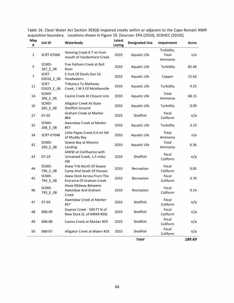
66

Table 16. Clean Water Act Section 303(d) impaired creeks within or adjacent to the Cape Romain NWR acquisition boundary. Locations shown in Figure 19. [Sources: EPA (2010), SCDHEC (2010)].

Map #

List ID Waterbody Latest Listing

Designated Use Impairment Acres

2 SCRT-07060 Venning Creek 0.7 mi from mouth of Vanderhorst Creek

2010 Aquatic Life Turbidity,

Total Ammonia

n/a

5 SCMD-267_E_06

Five Fathom Creek at Bull River

2010 Aquatic Life Turbidity 85.44

7 SCRT-02016_E_06

E Fork Of Devils Den Ck Headwaters

2010 Aquatic Life Copper 15.62

11 SCRT-01623_E_06

Tributary To Mathews Creek, 1 M S Of Mclellanville


14 SCMD-266_E_06

Casino Creek At Closure Line 2010 Aquatic Life Total

Ammonia 68.15

16 SCMD-265_E_06

Alligator Creek At State Shellfish Ground


27 07-02 Graham Creek at Marker #64

2010 Shellfish Fecal

Coliform n/a

32 SCMD-268_E_08

Awendaw Creek at Marker #57


34 SCRT-07048 Little Papas Creek 0.4 mi SW of Muddy Bay

2010 Aquatic Life Total

Ammonia n/a

42 SCMD-269_E_08

Sewee Bay at Moores Landing

2010 Aquatic Life Total

Ammonia 6.36

43 07-19 AIWW at Confluence with Unnamed Creek, 1.5 miles SW


Coliform n/a

44 SCMD-796_E_08

Aiww Trib North Of Sewee Camp And South Of Houses

2010 Recreation Fecal

Coliform 0.85

45 SCMD-794_E_08

Aiww Dock Across From The Entrance Of Graham Creek


Coliform 0.70

46 SCMD-793_E_08

Aiww Midway Between Awendaw And Graham Creek


Coliform 0.14

47 07-03 Awendaw Creek at Marker #57


Coliform n/a

48 06B-09 Dupree Creek - 500 FT N of New Dock (S. of MRKR #30)


Coliform n/a

49 06B-08 Casino Creek at Marker #29 2010 Shellfish Fecal

Coliform n/a

50 06B-07 Alligator Creek at Maker #26 2010 Shellfish Fecal

Coliform n/a

Total

189.69

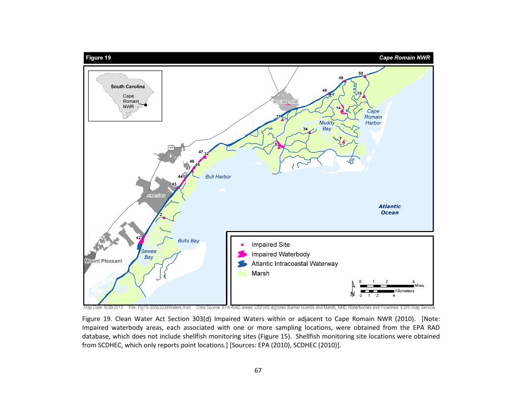
67

Figure 19. Clean Water Act Section 303(d) Impaired Waters within or adjacent to Cape Romain NWR (2010). [Note: Impaired waterbody areas, each associated with one or more sampling locations, were obtained from the EPA RAD database, which does not include shellfish monitoring sites (Figure 15). Shellfish monitoring site locations were obtained from SCDHEC, which only reports point locations.] [Sources: EPA (2010), SCDHEC (2010)].

70

5.4.3 Other Surface Water Quality Information

From 1999-2008, the SCECAP sampled several sites within or proximate to the refuge acquisition boundary (Table 15, Figure 16). All open water sites attained “good” water quality scores and several tidal creek locations were scored as “fair.” Sediment quality scores were mixed: tidal creek scores ranged from “good” to “poor,” while open water sites were scored as “good” and “fair.” Finally, all open water sites and most tidal creek sites achieved “good” biological condition scores, while a few tidal creek sites had “fair” and “poor” scores. In the 2007-2008 survey as in previous surveys, for all three indices (water quality, sediment quality, and biological condition), a higher proportion of tidal creek sites than open water sites along the South Carolina coast have been assessed in “fair” or “poor” condition (Bergquist et al. 2011). The SCDNR and SCDHEC are currently preparing the 2009-2010 report.

From April 2001 to July 2005 the NOAA Center for Coastal Environmental Health and Biomolecular Research (CCEHBR) implemented a water quality study to measure parameters that are indicative of anthropogenic and natural changes within the refuge (temperature, salinity, pH, DO and turbidity). A notable change in water quality occurred with the shift from dry to wet years. Periods of heavy rainfall, combined with freshwater releases from the Santee River, negatively influenced water quality in the refuge, particularly in the northern portion; a harmful algal bloom (HAB) occurred in Bulls Bay in April 2003 under those conditions. Water quality impacts were not limited to wet periods; instances of severe hypoxia (DO concentrations below 2 mg/L) were observed on seven occasions at four sampling locations, primarily during the summer months of dry years (Kracker and Meaburn 2006).

5.4.4 Groundwater Quality

Through its Source Water Assessment and Protection Program (SWAP), SCDHEC assesses all federally defined drinking water supply systems. Groundwater susceptibility assessments of the refuge’s water systems supplied by wells G10351 and G10256 were conducted in 2003 and 2006, respectively. Potential contaminant sources (PCS) were identified by reviewing SCDHEC files, site inspections and published reports on hydrogeology and aquifer tests. PCSs are defined by land-use or site-specific activities that could potentially release contaminants. The 2003 assessment found one PCS for nitrates and another for pathogens (SCDHEC 2003a), both ranked as low susceptibility. The 2006 assessment found two PCSs for petroleum products and one PCS for metals, both of which were also ranked as low susceptibility (SCDHEC 2006).

The Garris Landing supply well tested positive for bacterial contamination approximately 8 to 10 years ago (Dan Ashworth, written communication, November 6, 2012).

Studies indicate saltwater intrusion into the Black Creek aquifer in areas near the refuge (Wachob et al. 2009: Figure 9-8). Additionally, the refuge’s CCP indicates that groundwater levels on the refuge are rising closer to the surface as a result of sea-level rise (USFWS 2010b). Refuge staff has observed that hatching success in sea turtle nests has decreased due to groundwater intrusion on low lying beaches, and that saltwater intrusion is affecting vegetation composition on the barrier islands of the refuge (Sarah Dawsey, personal communication, January 28, 2013).

71

6 Water Law and Water Rights

Wachob et al. (2009) provide a fairly comprehensive discussion of South Carolina water law, from which the following very brief synopsis is drawn. The basic law governing natural watercourses (i.e., rivers and streams) in South Carolina is common-law riparian doctrine, which holds that the owner of land bounded or crossed by a natural watercourse has a property right to “reasonable use” of the water so long as that use does not adversely impact upstream or downstream property owners (e.g., by causing flooding) or interfere with the exercise of their riparian water rights. Corresponding rights for property owners adjacent to lakes, ponds, and marine waters are called littoral rights. General common law of littoral rights provides for access to and use of water in a natural body, but a landowner adjacent to an artificial lake or pond does not have littoral rights. Unlike many other states, South Carolina has not adopted a riparian-type common-law doctrine governing groundwater use, although the State has imposed reasonable-use restrictions on groundwater use by statute as described below.

New statutes have increased regulation of water use in South Carolina in recent years. The South Carolina Surface Water Withdrawal, Permitting, Use, and Reporting Act, enacted in 2010 (SC General Assembly 2010), requires that any person withdrawing surface water in excess of 3 million gallons (9.2 acre-feet ) in any month obtain a permit from and annually report water use to SCDHEC. With respect to groundwater, the Groundwater Use and Reporting Act (SC General Assembly 2000) requires that any person withdrawing more than 3 million gallons in any month to register their groundwater source(s) and report their use to SCDHEC. Within capacity use designation areas, groundwater withdrawals of over 3 million gallons in any month require a permit from the SCDHEC due to concerns about overuse and lowering of groundwater levels. Charleston County, where the refuge is located, is within the Trident Capacity Use Area (SCDHEC undated). Both groundwater and surface water withdrawals for the purpose of wildlife habitat management, however, are specifically exempted from regulation.

The tidal creeks, estuarine waters, and other navigable waters within the refuge boundary are owned by the State of South Carolina, but are managed as part of the refuge under 99-year lease agreement with the State of South Carolina signed in 1991 (Appendix A).

72

7 Assessment

7.1 Water Resource Issues of Concern

In this section, we highlight and briefly discuss what we see as the major water resources-related threats or issues of concern pertaining to the refuge. To provide context, we first briefly discuss the primary driver of threats to the refuge’s resource base—climate change impacts associated with sea-level rise—and then discuss specific threats or issues of concern in two categories: urgent or immediate issues (those for which impacts are already strongly manifest) and longer term issues.

A report on coastal impacts of climate change prepared as part of the 2013 National Climate Assessment states that:

“Sea level change and storms are dominant driving forces of coastal change as observed in the geologic record of coastal landforms. Increasingly, sea level rise will become a hazard for coastal regions because of continued global mean sea level rise, including possibly accelerated rates of rise that increase risk to coastal regions. As the global climate continues to warm and ice sheets melt, coasts will become more dynamic and coastal cities and low-lying areas will be increasingly exposed to erosion, inundation, and flooding… Most coastal landforms, such as barrier islands, deltas, bays, estuaries, wetlands, coral reefs, are highly dynamic and sensitive to even small changes in physical forces and feedbacks such as warming, storms, ocean circulation, waves and currents, flooding, sediment budgets, and sea level rise” (Burkett and Davidson 2012).

For many coastal regions composed of barrier islands, dunes, spits, sandy bluffs, and wetlands, such as Cape Romain NWR, erosion and inundation at highly variable rates will be the dominant response to sea-level rise and storms over this century and beyond. For some barrier islands and wetlands, higher sea-level rise scenarios will cause significant and irreversible changes including rapid landward migration and segmentation of some barrier islands, as well as disintegration and drowning of wetlands (Williams and Gutierrez 2009).

7.1.1 Urgent/Immediate Issues

1. Due to ongoing rapid shoreline erosion on the northeastern coast of Bulls Island, there is an imminent threat of breaching of the dike on the seaward side of the Jacks Creek impoundment (Figure 11), which would immediately and irrevocably convert the impoundment to an intertidal hydrologic regime, greatly reducing the available habitat that could be managed for waterfowl, wading birds, and shorebirds. Breaching of the dike would also threaten the interior freshwater impoundments, putting at risk the recent investments in WCS replacements and other water management infrastructure (Section 5.2.2, Appendix F) and endangering freshwater supplies utilized by all wildlife on the island. This is because breaching of the seaward dike would expose the much lower and less robust internal dikes separating Jacks Creek impoundment from the interior freshwater impoundments to direct tidal action and waves. Saltwater would intrude into the freshwater pools regularly as moderate storms would be capable of generating waves that could overtop the lower internal dikes. In addition, severe erosion would likely occur on the dikes, especially around the water control structures, as they were not designed for regular daily tidal flow.

2. Rapid erosion of barrier islands due to sea-level rise, intense storms, and possible intensification of wave energy and storm surge is reducing and threatens to eliminate nesting, foraging, and resting habitat for Federal Trust species including threatened loggerhead sea turtles, threatened piping

73

plover, red knot; currently proposed for listing with proposed critical habitat on the refuge), other species of shorebirds whose populations are in significant decline, seabirds, and habitat for endangered seabeach amaranth. A decrease in the productivity of beach nesting species has been observed due to loss of habitat and saltwater intrusion, particularly on Cape and Lighthouse Islands. Shoreline erosion on these islands has likely been exacerbated by:

decreased sediment supply due to dam construction in the Santee River basin circa 1940,

disruption of seaward sediment transport in the Santee River estuary and Winyah Bay due to dredging to maintain shipping channels and diversion of a portion of historic river flows into the AIW, and

disruption of generally southward longshore sediment transport along the coast by dredging (Santee delta) and jetties (Winyah Bay entrance).

Exposure of formerly protected salt marsh and islands has resulted when barrier islands (Cape Island, Lighthouse Island) erode, exposing vulnerable shorelines to the erosive forces of tides and wave action. For example, in 2009, when Sandy Point eroded and disappeared beneath the water, the land lying north and west of Sandy Point, bounded on the east by Five Fathom Creek, and opposite White Banks, began to rapidly erode, eliminating an approximately 120-acre unnamed island.

3. Relative sea-level rise (exacerbated by the anthropogenic sediment transport disruptions discussed above) is inundating and fragmenting the 29,000-acre Cape Romain Class I Wilderness Area through conversion of marsh to tidal creek and the resulting fragmentation of the marsh platform. The marsh is vital nursery habitat for juvenile fish, crabs, and shrimp that take refuge among the vegetation for protection from predators. These species are the foundation of the food chain upon which coastal species are dependent. In addition to habitat loss and fragmentation, these changes lead to increased salinity in refuge estuaries. Wilderness designation limits options for active management response even if financial resources were not limiting.

4. The supply of freshwater for habitat management in the impoundments on Bulls Island is unreliable due to the dependence on rainfall. In dry years there is often insufficient freshwater to maintain desired conditions (e.g., water levels, salinity, waterfowl food plants) in the impoundments, particularly during the summer and early fall. Groundwater is a potential source for supplemental freshwater; however, existing and previous water supply wells on Bulls Island that have tapped the Gordon aquifer have generally yielded limited quantities of poor quality water (high sulfur and/or coliform bacteria). The Charleston aquifer, which underlies Bulls Island at depths between approximately 1600 to 1800 feet (Campbell and Coes 2010), provides a potential source of groundwater supply. A well completed in the Charleston aquifer would likely be capable of producing 500 to 1,500 gpm (Bruce Campbell, written communication, June 17, 2013), although the water produced would likely have a chloride concentration near the 250 mg/L approximate taste threshold that is commonly used to define the freshwater/saltwater contact (Wachob et al. 2009).

5. In addition to limited and unreliable freshwater availability, water management infrastructure limitations currently limit the ability of the refuge to move water among the Bulls Island impoundments. While most of the WCS on the refuge have recently been replaced, ditches linking the impoundments have not been maintained due to a lack of personnel and equipment and are in need of clearing and/or re-grading to restore them to their original dimensions and capacity. Additionally, water movement in the current system relies wholly on tidal water level fluctuations and gravity-driven flow. The refuge lacks any active capacity (e.g., high-capacity pumps) to move

74

water where it is needed. This further limits the capacity of refuge staff to manipulate water and salinity levels in the impoundments to control undesirable plant species and maintain desired habitat conditions for waterfowl. The refuge also currently lacks adequate staff to manage water levels and habitat conditions in the impoundments as actively as would be desirable.

7.1.2 Longer-Term Issues

1. Hard armoring of adjacent and nearby properties as a response to rising sea levels reduces the capacity for habitat shifts to occur in the future. The existence of high density development that must be protected through shoreline hardening, beach nourishment or other measures, as on the barrier islands to the south of the refuge (e.g., Isle of Palms), prevents shoreline migration, interfering with the ability of neighboring coastal habitats and ecosystems to shift and change in response to sea-level rise.

2. Urban development and associated infrastructure (e.g., subdivisions, golf courses, roads), failing septic systems, and deforestation on the mainland have and will continue to contribute point and non-point source pollution to receiving waters within the refuge, adversely impacting water quality. Water quality impacts from these sources include elevated turbidity (sediment load), nutrients, metals (often bound to sediments), organic contaminants such as PAHs, and human pathogens. In addition, the high levels of impervious land cover associated with urban development yields flashy (rapidly varying) stormwater runoff that leads to highly variable water quality (SC Sea Grant Consortium 2008). Nutrient-laden stormwater runoff can reduce estuarine salinity levels and lead to harmful algal blooms, such as occurred in April 2003 in Bulls Bay (Kracker and Meaburn 2006).

7.2 Needs and Recommendations

1. To mitigate for the eventual breaching of the seaward dike enclosing the Jacks Creek impoundment as a result of continued erosion, construction of a cross-dike through Jacks Creek impoundment has been proposed at an estimated cost of $3 million (USFWS 2010b, Appendix G). This would differ from previous patch dikes in that it would be set well back from the current dike, essentially cutting the impoundment in half. The ocean half would be allowed to breach and convert to salt marsh, while the inner half would be managed as a brackish impoundment for waterfowl, shorebirds and wading birds. By setting the dike back, it is anticipated that construction of the proposed cross-dike would allow the refuge to continue to manage the remaining impoundments for migratory bird habitat for at least 20 years. A decision on whether to proceed with this proposed project will need to consider available financial resources, other priorities identified in the CCP (USFWS 2010b), recent investments in water management infrastructure on Bulls Island (Appendix F), and management alternatives identified in the HGM that is currently in progress at the refuge (scheduled to be completed by the end of 2013). If a decision is made to proceed with the cross-dike, it is critically important that it be completed before the existing seaward portion of Jacks Creek dike is breached, which is expected to occur sometime within the next few years given current shoreline erosion rates.

2. To provide a reliable source of freshwater for habitat management, a deep (~1,800 ft) groundwater supply well tapping the Charleston aquifer could be drilled on Bulls Island. Such a well would likely yield 500 to 1,500 gpm of water with a chloride concentration of around 250 parts per million (ppm) and a total salinity in the neighborhood of 450 ppm, well below the brackish water threshold of 1,000 ppm. It is possible that a well completed in the Charleston aquifer would be a flowing well and would not require a pump. If a pump is required, a high-capacity diesel powered pump or electric pump (requiring 3-phase electrical service) could be used. As a point of reference with

75

respect to the likely cost of such a well, Mount Pleasant Water Works recently replaced a production well completed in the Charleston aquifer at a cost of approximately $750,000 (Bruce Campbell, personal communication, June 19, 2013.)

3. An updated water management plan should be prepared by a qualified contractor or partner organization with the necessary hydrologic and engineering expertise. The plan should include a field-based assessment of water management capabilities, including a survey of elevations and grades of WCS and conveyance channels, and should make specific recommendations of improvements or maintenance (e.g., clearing or re-grading of ditches, acquisition of portable high-volume low-head pumps, etc.) needed to provide satisfactory water management capabilities. The plan should consider potential impacts of sea-level rise on the water management system as a whole. In particular, it should consider whether improvements to the conveyance system and connectivity between the impoundments increases the vulnerability of the inner impoundments (Pools 1, 2 and 3, Big Pond, House Pond, and Lower Summerhouse Pond) to breaching or increased salinity should any of the outer impoundments fail or become more saline (e.g., due to more frequent overwash of dikes during storms) as a result of continued sea-level rise.

4. A detailed water monitoring plan should be developed and implemented, either as part of the Inventory and Monitoring Plan or water management plan for the refuge or as a stand-alone document. Water monitoring efforts are tied to critical baseline information needs in the adaptive management framework, targeting ecological integrity while meeting refuge-level, regional and national Water Resources Inventory and Monitoring Goals and Objectives (USFWS 2010a, USFWS 2013). Specific tasks should include the following elements:

Monitoring of water levels and basic water quality parameters (temperature, pH, salinity, and DO) in the Bulls Island impoundments. Depending upon available resources, it would also be helpful to install some shallow wells in the vicinity of the impoundments to monitor seasonal fluctuations and long-term changes (e.g., in response to sea-level rise) in groundwater levels and groundwater quality (particularly salinity) and to assess potential impacts on water levels and water quality in the impoundments.

Water quality monitoring (temperature, pH, salinity, turbidity, DO, and nutrients) in tidal channels at selected locations—ideally at several fixed locations and several randomly selected temporary (rotating) locations.

Ideally, supplement water quality monitoring at fixed points with seasonal synoptic surveys to better characterize spatial water quality patterns (and seasonal variation in those patterns).

Continuous tidal water level monitoring at one or more fixed locations (e.g., Garris Landing).

5. Implementation of the plans described in Recommendations 3 and 4 above (i.e., managing water levels and habitat conditions in the Bulls Island impoundments and conducting water monitoring) would require additional staff resources. It is estimated that these tasks would require approximately 0.25-0.5 FTE by a hydrologic technician or similarly qualified staff person to fully implement.

6. Obtain full LiDAR coverage for the refuge and adjacent mainland areas when it becomes available. Given the inescapable reality of sea-level rise, complete high-quality LiDAR data are essential for refuge planning purposes. LiDAR data for this area were acquired by the South Carolina LiDAR Consortium in 2009, but release of the data has been delayed due to data processing issues. Reprocessing of the LiDAR data by a new vendor is currently in progress, and the reprocessed data

76

are scheduled to be delivered for internal review in December 2013 (Jim Scurry, personal communication, October 24, 2013). Assuming satisfactory resolution of the data quality issues, the data will become publicly available via the SCDNR website (http://www.dnr.sc.gov/GIS/lidar.html) once the data review has been completed in early 2014. If data quality issues cannot be resolved or the data prove to be inadequate for refuge planning needs, the refuge should explore opportunities to partner with other stakeholders (e.g., local and state government agencies, NGOs, Frances Marion National Forest, etc.) to obtain suitable LiDAR data.

7. Develop and implement a plan to monitor sea-level rise impacts on coastal erosion on barrier islands and on fragmentation and conversion of tidal marsh. Elements of the plan could include the following:

Once LiDAR data have been obtained, perform a new SLAMM analysis using LiDAR-derived elevation data and customized land cover data (e.g., modified NWI land cover with ground-truthed cover classes). The analysis area should extend several miles inland from the existing refuge boundary and ideally should include the Santee River delta.

Continued monitoring of barrier island and shoreline erosion using aerial imagery and ground-based measurements. Expand the geospatial analysis beyond the four primary barrier islands to all land and marsh on the refuge. Develop a baseline analysis and monitor regularly as new imagery becomes available to track accretion, erosion, and tidal creek expansion.

Explore funding and/or partnership opportunities to install additional SET stations to monitor marsh accretion, subsidence, and surface elevation changes closer to the mainland in high marsh.

8. In partnership with the U.S. Forest Service, state agencies, and NGOs, develop a long-term, landscape-scale strategy for responding to sea-level rise. Given the inevitability of continuing sea-level rise and landward shoreline migration over the next several centuries, tidal marsh, wetland, and terrestrial habitats within the existing refuge footprint will certainly shrink and ultimately may disappear altogether. Any long-term planning effort, either at the refuge, landscape, or regional scale, will need to confront this reality. Connecting protected areas that extend from refuge estuaries to the Francis Marion National Forest will create corridors that will allow for species and habitat migration in the future. Because continued rapid development on the mainland adjacent to the refuge could severely limit future management options involving new land acquisition or easements within the next decade, it is essential to develop and begin implementing such an adaptation strategy soon as possible.

9. Build upon existing partnerships and explore new partnership opportunities with other federal and state agencies, NGOs, and academic institutions to carry out relevant research for habitat and species management and baseline data needs in light of continued urban development, sea-level rise, and climate change impacts. Examples of identified research needs include the following:

Examine the effects of groundwater inundation and saltwater intrusion due to sea-level rise on sea turtle nests in the refuge.

Replicate the Bulls Island vegetation study by Mixon (2002) to show changes in habitat composition from saltwater intrusion.

77

8 Literature Cited

[AMS] American Meteorological Society. 2012. American Meteorological Society Glossary of Meteorology [Internet]. Accessed 8 March 2013. Available from: http://glossary.ametsoc. org/wiki/Main_Page.

Aucott, W.R. 1996. Hydrology of the Southeastern Coastal Plain aquifer system in South Carolina and parts of Georgia and North Carolina: U.S. Geological Survey Professional Paper 1410-E, 83 p. Accessed 20 November 2012. Available from: http://pubs.er.usgs.gov/publication/pp1410E.

Aucott, W. R., and G.K. Speiran. 1985. Ground-water flow in the Coastal Plain aquifers of South Carolina. Ground Water 23(6): 736-745.

Barnhardt, W.A., editor. 2009. Coastal change along the shore of northeastern South Carolina—the South Carolina coastal erosion study: U.S. Geological Survey Circular 1339. 77 p.

Barth, M.C., and J.G. Titus, editors. 1984. Greenhouse Effect and Sea Level Rise: A Challenge for This Generation. New York: Van Nostrand Reinhold Company.

Bergquist, D.C., R.F. Van Dolah, G.H.M. Riekerk, M.V. Levisen, S.E. Crowe, D.E. Chestnut, W. McDermott, M.H. Fulton, E. Wirth, and J. Harvey. 2011. The Condition of South Carolina’s Estuarine and Coastal Habitats During 2007-2008: Technical Report. Charleston, SC: South Carolina Marine Resources Division. Technical Report No. 106. 64 p. Accessed 4 May 2012. Available from: http://www.dnr.sc.gov/marine/scecap/surveyperiods/20072008TechnicalReport.pdf.

Burkett, V.R. and M.A. Davidson, editors. 2012. Coastal Impacts, Adaptation and Vulnerability: A Technical Input to the 2012 National Climate Assessment. Cooperative Report to the 2013 National Climate Assessment. 150 p.

Caldwell, R.J., H.P. Mizzell, and M. Brown. 2005. Spatial distribution of tropical cyclone induced precipitation and operational applications in South Carolina [Internet]. South Carolina State Climatology Office, Columbia, South Carolina. 7 p. Accessed 11 March 2013. Available from: http://www.dnr.sc.gov/climate/sco/Tropics/TropicalRainfall/tropicprecip/abstract.pdf

Campbell, B.G., and A.L. Coes, editors. 2010. Groundwater availability in the Atlantic Coastal Plain of North and South Carolina: U.S. Geological Survey Professional Paper 1773. 241 p., 7 pls. Accessed 29 February 2012. Available from: http://pubs.usgs.gov/pp/1773/

[CCSP] Climate Change Science Program. 2009. Coastal Sensitivity to Sea-Level Rise: A Focus on the Mid-Atlantic Region. A report by the U.S. Climate Change Science Program and the Subcommittee on Global Change Research. [James G. Titus (Coordinating Lead Author), K. Eric Anderson, Donald R. Cahoon, Dean B. Gesch, Stephen K. Gill, Benjamin T. Gutierrez, E. Robert Thieler, and S. Jeffress Williams (Lead Authors)]. U.S. Environmental Protection Agency, Washington D.C., USA. 320 p.

Chan, S. 2008. A plan for monitoring shorebirds during the non-breeding season in Bird Monitoring Region South Carolina - BCR 27 [Internet]. Manomet Center for Conservation Sciences. Accessed 23 April 2012. Available from: ftp://ftp.manomet.org/Prism/South Carolina BCR 27.doc.

Church, J.A. and J.M. Gregory (Coordinating Lead Authors), P. Huybrechts, M. Kuhn, K Lambeck, M.T. Nhuan, D. Qin, and P.L. Woodworth (Lead Authors), and 28 others, 2001: Changes in Sea Level. In: Climate Change 2001: The Scientific Basis. Contribution of Working Group I to the Third Assessment Report of the Intergovernmental Panel on Climate Change [Houghton, J.T.,Y. Ding,

http://glossary.ametsoc.org/wiki/Main_Page

http://glossary.ametsoc.org/wiki/Main_Page

http://pubs.er.usgs.gov/usgspubs/pp/pp1410E

http://pubs.er.usgs.gov/usgspubs/pp/pp1410E

http://pubs.er.usgs.gov/publication/pp1410E

http://www.dnr.sc.gov/marine/scecap/surveyperiods/20072008TechnicalReport.pdf

http://www.dnr.sc.gov/climate/sco/Tropics/TropicalRainfall/tropicprecip/abstract.pdf

http://pubs.usgs.gov/pp/1773/

ftp://ftp.manomet.org/Prism/South Carolina BCR 27.doc

78

D.J. Griggs, M. Noguer, P.J. van der Linden, X. Dai, K. Maskell, and C.A. Johnson (eds.)]. Cambridge University Press, Cambridge, United Kingdom and New York, NY, USA, 881p.

Clough, J. S., R.A. Park, and R. Fuller. 2010. SLAMM 6 beta Technical Documentation [Internet]. Accessed March 2013. Available from: http://warrenpinnacle.com/prof/SLAMM.

Cowardin, L.M., V. Carter, F.C. Golet, and E.T. LaRoe. 1979. Classification of wetlands and deepwater habitats of the United States. U.S. Fish and Wildlife Service. Washington, D.C.

Dowsett, H.J. and T.M. Cronin. 1990. High eustatic sea level during the middle Pliocene: Evidence from the southeastern U.S. Atlantic Coastal Plain. Geology. 18: 435-438.

Ehman, J. 2008. Data report on SLAMM model results for ten National Wildlife Refuges in South Carolina and Georgia: Cape Romain NWR, South Carolina.

[EPA] U.S. Environmental Protection Agency. 2008. Draft guidance on the development, evaluation, and application of environmental models. Council for Regulatory Environmental Modeling, U.S. Environmental Protection Agency, Washington, D.C. August 2008.

[EPA] U.S. Environmental Protection Agency. Reach Access Database (RAD). 2010. South Carolina 303(d) Impaired Waterbodies [Internet]. Accessed March 2012. Available from: http://epamap32.epa.gov/radims/.

Farnsworth, R.K., and E.S. Thompson. 1982. Mean Monthly, Seasonal, and Annual Pan Evaporation for the United States. NOAA Technical Report NWS 34. Office of Hydrology, National Weather Service, Washington, D.C. Available from: http://www.nws.noaa.gov/oh/hdsc/PMP_related_ studies/TR34.pdf

Farnsworth, R.K., E.S. Thompson, and E. L. Peck. 1982. Evaporation Atlas for the Contiguous 48 United States. NOAA Technical Report NWS 33. Office of Hydrology, National Weather Service, Washington, D.C. Available from: http://www.nws.noaa.gov/oh/hdsc/PMP_related_studies/ TR33.pdf

[FERC] Federal Energy Regulatory Commission. 2007. Final Environmental Impact Statement (FEIS) for the Santee Cooper Hydroelectric Project located in Berkeley, Calhoun, Clarendon, Orangeburg, and Sumpter Counties, South Carolina. (Project No. 199-205). October 26, 2007. Available from: http://www.ferc.gov/industries/hydropower/enviro/eis/2007/10-26-07.asp

Girvetz, E.H., C. Zganjar, G.T. Raber, E.P. Maurer, P. Kareiva, P. and J.J. Lawler. 2009. Applied Climate-Change Analysis: The Climate Wizard Tool. PLoS ONE 4(12): e8320. DOI: 10.1371/journal. pone.0008320.

Grinsted, A., J.C. Moore, and S. Jevrejeva. 2009. Reconstructing sea level from paleo and projected temperatures 200 to 2100AD. Climate Dynamics 34 (4): 461-472. Available from: ftp://ftp.soest.hawaii.edu/coastal/Climate Articles/Grinsted Jevrejeva 2009 SLR.pdf

Gordon, D.H., Gray, B.T., Perry, R.D., Provost, M.B., Strange, T.H. and R.K. Williams. 1989. South Atlantic coastal wetlands. In: Smith, L.M., R.L. Pederson, and R.M. Kaminski, editors. Habitat Management for Migrating and Wintering Waterfowl in North America. Texas Tech University Press. 560 p.

Gutowski, W.J., G.C. Hegerl, G.J. Holland, T.R. Knutson, L.O. Mearns, R.J. Stouffer, P.J.Webster, M.F. Wehner, and F.W. Zwiers. 2008. Causes of Observed Changes in Extremes and Projections of Future Changes. In: Karl, T.R., G.A. Meehl, C.D. Miller, S.J. Hassol, A.M. Waple, W.L. Murray, editors. Weather and Climate Extremes in a Changing Climate. Regions of Focus: North America,

http://warrenpinnacle.com/prof/SLAMM

http://epamap32.epa.gov/radims/

http://www.nws.noaa.gov/oh/hdsc/PMP_related_studies/TR34.pdf




http://www.ferc.gov/industries/hydropower/enviro/eis/2007/10-26-07.asp

ftp://ftp.soest.hawaii.edu/coastal/Climate Articles/Grinsted Jevrejeva 2009 SLR.pdf

79

Hawaii, Caribbean, and U.S. Pacific Islands. A Report by the U.S. Climate Change Science Program and the Subcommittee on Global Change Research, Washington, D.C.

Harder, S.V., Gawne, C.E., Gellici, J.A. and A. Wachob. 2012. Ground-water Levels in South Carolina, 2006-2010. State of South Carolina Department of Natural Resources Land, Water and Conservation Division Water Resources Report 50. Accessed 21 November 2012. Available from: http://www.dnr.sc.gov/water/hydro/HydroPubs/pdf/Report_50_WL_Data.pdf.

Harwell, S.L., Park, A.D., Hockensmith, B.L. and C.E. Gawne. 2004. Water Resources Data for South Carolina 2000-2001. State of South Carolina Department of Natural Resources Land, Water and Conservation Division Water Resources Report 31. Accessed 21 November 2012. Available from: http://www.dnr.sc.gov/lwc/pubs/pdfs/Report31.pdf.

Hayes, M.O. and J. Michel. 2008. A Coast for All Seasons: A Naturalist's Guide to the Coast of South Carolina. Pandion Books, Columbia, SC. 285 p., 165 color plates.

Hockensmith, B.L. 2004. Flow and salinity characteristics of the Santee River Estuary, South Carolina. South Carolina Department of Natural Resources Water Resources Report 35. Available from: h p://www.dnr.sc.gov/water/img/Report35.pdf .

Hockensmith, B.L. 2012a. Potentiometric Surface of the Middendorf Aquifer in South Carolina, November 2009. South Carolina Department of Natural Resources, Water Resources Report 51. Available from: http://www.dnr.sc.gov/water/hydro/HydroPubs/pdf/Report_51_Middendorf_2009.

pdf.

Hockensmith, B.L. 2012b. Potentiometric Surface of the Black Creek Aquifer in South Carolina, November 2009. South Carolina Department of Natural Resources, Water Resources Report 52. Available from: http://www.dnr.sc.gov/water/hydro/HydroPubs/pdf/Report_52_Black_Creek_

2009.pdf.

Holland, J. and P.J. Webster. 2007. Heightened tropical cyclone activity in the North Atlantic: natural variability or climate trend? Philosophical Transactions of the Royal Society A. DOI: 10.1098/ rsta.2007.2083.

Hoyt, J.H. 1968. Geology of the Golden Isles and lower Georgia coastal plain. p. 18-34. In: D.S. Maney, F.C. Marland, and C.B. West, editors. Conference on the Future of the Marshlands and Sea Islands of Georgia. Oct. 13-14, 1968. Georgia Natural Areas Council and Coastal Area Planning and Development Commission.

Hughes, Z.J., D.M. FitzGerald, C.A. Wilson, S.C. Pennings, K. Wieski, and A. Mahadevan. 2009. Rapid headward erosion of marsh creeks in response to relative sea level rise. Geophysical Research Letters, 36, L03602. DOI:10.1029/2008GL036000.

[IPCC] Intergovernmental Panel on Climate Change. 2007. Contribution of Working Group I to the Fourth Assessment Report of the Intergovernmental Panel on Climate Change. Solomon, S., D. Qin, M. Manning, Z. M. Chen, K.B. Marquis, M. Averyt, M. Tignor, and H.L. Miller (editors.) Cambridge University Press, Cambridge, United Kingdom and New York, NY, USA. 996 p.

Kjerfve, B. 1976. The Santee-Cooper: a study of estuarine manipulations. Estuarine Processes 1: 44-56.

Knutson, T.R. and R.E. Tuleya. 2008. Tropical cyclones and climate change: revisiting recent studies at GFDL. In: Diaz, H. and R. Murnane, editors. Climate Extremes and Society. Cambridge University Press, Cambridge, UK, and New York, p. 120-144.

http://www.dnr.sc.gov/water/hydro/HydroPubs/pdf/Report_50_WL_Data.pdf

http://www.dnr.sc.gov/lwc/pubs/pdfs/Report31.pdf

http://www.dnr.sc.gov/water/img/Report35.pdf‎

http://www.dnr.sc.gov/water/img/Report35.pdf‎

http://www.dnr.sc.gov/water/hydro/HydroPubs/pdf/Report_51_Middendorf_2009.pdf

http://www.dnr.sc.gov/water/hydro/HydroPubs/pdf/Report_51_Middendorf_2009.pdf

http://www.dnr.sc.gov/water/hydro/HydroPubs/pdf/Report_52_Black_Creek_2009.pdf

http://www.dnr.sc.gov/water/hydro/HydroPubs/pdf/Report_52_Black_Creek_2009.pdf

80

Kracker, L.M. and G.M. Meaburn. 2006. Spatial and temporal characterization of water quality at Cape Romain National Wildlife Refuge. NOAA Technical Memorandum NOS NCCOS 33. 36 p.

Kunkel, K.E., P.D. Bromirski, H.E. Brooks, T. Cavazos, A.V. Douglas, D.R. Easterling, K.A. Emanuel, P.Y.A. Groisman, P.Y.A., G.J. Holland, T.R. Knutson, J.P. Kossin, P.D. Komar, D.H. Levinson, and R.L. Smith. 2008. Observed Changes in Weather and Climate Extremes. In: Karl, T.R., G.A. Meehl, C.D. Miller, S.J. Hassol, A.M. Waple, and W.L. Murray, editors. Weather and Climate Extremes in a Changing Climate. Regions of Focus: North America, Hawaii, Caribbean, and U.S. Pacific Islands. A Report by the U.S. Climate Change Science Program and the Subcommittee on Global Change Research, Washington, D.C.

Lewis, J.D. Undated. South Carolina IntraCoastal Waterway [Internet]. Accessed 17 September 2012. Available from: http://www.coastalguide.com/IntraCoastalWaterway/SC-IntraCoastal Waterway.shtml.

Mathews , T.D., F.W. Stapor, Jr., C.R. Richter, J.V. Miglarese, M.D. McKenzie, and L.A. Barclay, editors. 1980. The ecological characterization of the sea island coastal region of South Carolina and Georgia. Vol. 1: Physical features of the characterization area. U.S. Fish and Wildlife Service FWS/OBS-79/40, 212 p.

Menne, M.J., C.N. Williams, Jr., and R.S. Vose. Undated. United States Historic Climatology Network: Long-Term Daily and Monthly Climate Records from Stations Across the Contiguous United States [Internet]. National Climatic Data Center, National Oceanic and Atmospheric Administration. Accessed November 2012. Available from: http://cdiac.ornl.gov/epubs/ndp/ ushcn/ushcn.html.

Miller, E.N. 1971. Soil Survey of Charleston County, South Carolina. Soil Conservation Service. 78 p.

Miller, J.A. 1992. Summary of the hydrology of the Southeastern Coastal Plain aquifer system in Mississippi, Alabama, Georgia, and South Carolina: U.S. Geological Survey Professional Paper 1410-A. 38 p.

Miller, K.G., M.A. Kominz, J. V. Browning, J.D. Wright, G.S. Mountain, M.E. Katz, P.J. Sugarman, B.S. Cramer, N. Christie-Blick, and S.F. Pekar 2005. The Phanerozoic record of global sea-level change. Science. 310:1293-1298.

Mixon, W.D. 2002. Maritime Forest Habitat Dynamics on Bulls Island, Cape Romain National Wildlife Refuge Following Hurricane Hugo. Master of Science thesis. Clemson University.

Morris, J.T., P.V. Sundareshwar, C.T. Nietch, B. Kjerfve, and D.R. Cahoon. 2002. Response of coastal wetlands to rising sea level. Ecology 83(10): 2869-2877. Available from: http://www.ias.sdsmt.edu/staff/sundareshwar/Reprints/morris%20et%20al%202002.pdf.

Morton, R.A. and T.L. Miller. 2005. National assessment of shoreline change: Part 2: Historical shoreline changes and associated coastal land loss along the U.S. southeast Atlantic coast. U.S. Geological Survey Open-File Report 2005-1401.

[NADP] National Atmospheric Deposition Program. Undated. NADP/NTN Monitoring Location SC05 [Internet]. Accessed 4 December 2012. Available from: http://nadp.sws.uiuc.edu/sites/ siteinfo.asp?id=SC05.

[NOAA] National Oceanic and Atmospheric Administration. 1999. Hurricane Basics [Internet]. Accessed May 2013. Available from: http://hurricanes.noaa.gov/pdf/hurricanebook.pdf

http://www.coastalguide.com/IntraCoastalWaterway/SC-IntraCoastalWaterway.shtml

http://www.coastalguide.com/IntraCoastalWaterway/SC-IntraCoastalWaterway.shtml

http://cdiac.ornl.gov/epubs/ndp/ushcn/ushcn.html

http://cdiac.ornl.gov/epubs/ndp/ushcn/ushcn.html

http://www.ias.sdsmt.edu/staff/sundareshwar/Reprints/morris%20et%20al%202002.pdf

http://nadp.sws.uiuc.edu/sites/siteinfo.asp?id=SC05

http://nadp.sws.uiuc.edu/sites/siteinfo.asp?id=SC05

http://hurricanes.noaa.gov/pdf/hurricanebook.pdf

81

[NOAA] National Oceanic and Atmospheric Administration. Undated. Tides and Currents website [Internet]. Accessed April 2012. Available from: http://tidesandcurrents.noaa.gov/.

Patterson, G.G., T.W. Cooney, and R.M. Harvey. 1996. Sediment Transport and Deposition in Lakes Marion and Moultrie, South Carolina, 1942-1985. U.S. Geological Survey Water-Resources Investigations Report 95-4236. 73 p.

[PRISM] Parameter-elevation Regressions on Independent Slopes Model. 2010. PRISM Climate Data [Internet]. Accessed 3 February 2012. Available from: http://www.prism.oregonstate.edu/. [Point data downloaded from http://prismmap.nacse.org/nn/ for geographic coordinates (-79.593201, 32.997434).]

Purvis, J. C., W. Tyler, and S. Sidlow. 1986. Hurricanes affecting South Carolina: South Carolina State Climatology Office Report G26. 19 p.

Raymo, M.E., J.X. Mitrovica, M.J. O’Leary, R.M. DeConto, and P.J. Hearty. 2011. Departures from eustasy in Pliocene sea-level records. Nature Geoscience 4:328-332. DOI: 10.1038/NGEO1118.

Riggs, S.R., D.V. Ames, S.J. Culver, and D.J. Mallinson. 2011. The Battle for North Carolina’s Coast: Evolutionary History, Present Crisis, and Vision for the Future. University of North Carolina Press, Chapel Hill. 160 p.

Rotzoll, K., and C.H. Fletcher. 2012 Assessment of groundwater inundation as a consequence of sea-level rise. Nature Climate Change 3: 477-481. DOI: 10.1038/NCLIMATE1725.

[SCDAH] South Carolina Department of Archives and History. 1979. National Register of Historic Places Inventory Nomination Form for Santee Canal [Internet]. Accessed 16 April 2013. Available from: http://www.nationalregister.sc.gov/berkeley/S10817708022/index.htm.

[SCDHEC] South Carolina Department of Health and Environmental Control. 2002. South Carolina Ambient Groundwater Monitoring Network 2002 Annual Report: Catawba and Santee Basins [Internet]. Accessed 23 April 2012. Available from: www.scdhec.gov/environment/water/docs/amb2002.pdf.

[SCDHEC] South Carolina Department of Health and Environmental Control. 2003a. Source Water Assessment for Cape Romain National Wildlife Refuge Office (Water System 1070678, Charleston County) [Internet]. April 23, 2003. Accessed April 2012. Available from: http://www.scdhec.gov/environment/water/docs/charlestonswp/1070678r.pdf.

[SCDHEC] South Carolina Department of Health and Environmental Control. 2003b. South Carolina Ambient Groundwater Monitoring Network 2003 Annual Report: Pee Dee Basin [Internet]. Accessed 21 November 2012. Available from: http://www.scdhec.gov/environment/water/docs/amb2003.pdf

[SCDHEC] South Carolina Department of Health and Environmental Control. 2006. Source Water Assessment for Cape Romain National Wildlife Refuge (Water System 1070653, Charleston County) [Internet]. June 1, 2006. Accessed April 2012. Available from: http://www.scdhec.gov/environment//water/docs/charlestonswp/1070653r.pdf

[SCDHEC] South Carolina Department of Health and Environmental Control. 2008. South Carolina Groundwater Contamination Inventory. Technical Report #002-08 [Internet]. Accessed 23 April 2012. Available from: http://www.scdhec.gov/environment/water/gwci/gwci.pdf.

[SCDHEC] South Carolina Department of Health and Environmental Control. 2010. The State of South Carolina’s 2010 Integrated Report. [Internet]. Accessed 4 November 2013. Available from:

http://tidesandcurrents.noaa.gov/station_retrieve.shtml?type=Tide+Data

http://www.prism.oregonstate.edu/

http://prismmap.nacse.org/nn/

http://www.nationalregister.sc.gov/berkeley/S10817708022/index.htm


http://www.scdhec.gov/environment/water/docs/charlestonswp/1070678r.pdf


http://www.scdhec.gov/environment/water/docs/charlestonswp/1070653r.pdf

http://www.scdhec.gov/environment/water/gwci/gwci.pdf

82

https://www.scdhec.gov/environment/water/tmdl/docs/tmdl_10-303d.pdf and https://www.scdhec.gov/environment/water/tmdl/docs/tmdl_10-305b.pdf.

[SCDHEC] South Carolina Department of Health and Environmental Control. 2012a. State of South Carolina Monitoring Strategy for Calendar Year 2012 [Internet]. Technical Report No. 102J-12. Accessed April 2012. Available from: http://www.scdhec.gov/environment/water/docs/strategy. pdf.

[SCDHEC] South Carolina Department of Health and Environmental Control. 2012b. R.61-68, Water Classifications and Standards [Internet]. Bureau of Water, S.C. Department of Health and Environmental Control, Columbia, SC. Accessed November 2012. Available from: http://www.scdhec.gov/environment/water/regs/R.61-68.pdf

[SCDHEC] South Carolina Department of Health and Environmental Control. 2012c. R.61-69, Classified Waters [Internet]. Bureau of Water, S.C. Department of Health and Environmental Control, Columbia, SC. Accessed November 2012. Available from: http://www.scdhec.gov/environment/ water/regs/R.61-69.pdf

[SCDHEC] South Carolina Department of Health and Environmental Control. 2012d. The State of South Carolina Integrated Report for 2012. Part I: Section 303(d) List of Impaired Waters [Internet]. Available from : http://www.scdhec.gov/environment/water/tmdl/ .

[SCDHEC] South Carolina Department of Health and Environmental Control. Undated. Map of Capacity Use Areas [Internet]. Accessed 3 May 2012. Available from: http://www.scdhec.gov/environment/water/docs/gw_capusem.pdf.

[SCDNR] South Carolina Department of Natural Resources. 2000. South Carolina Maps and Aerial Photographic Systems (SC MAPS) Teaching Manual, 4th Edition. Accessed 17 September 2012 from: http://www.clemson.edu/ces/geolk12/scmaps/Manual/sc_maps_teaching_manual.html

[SCDNR] South Carolina Department of Natural Resources. Undated-a. DNR GIS Data Clearinghouse [Internet]. Accessed April 2012. Available at http://www.dnr.sc.gov/GIS/gisdownload.html

[SCDNR] South Carolina Department of Natural Resources. Undated-b. South Carolina Coastal Plain

Water Well Records – Charleston County [Internet]. Accessed 26 November 2012. Available

from: http://dnr.sc.gov/water/hydro/WellRecords/Wells_main.htm.

[SCDNR] South Carolina Department of Natural Resources. Undated-c. South Carolina Department of

Natural Resources GIS Data Resources, LiDAR and Related Data Products [Internet]. Accessed 8

July 2013. Available from: http://www.dnr.sc.gov/GIS/lidar.html.

[SCDNR State Climatology Office] South Carolina Department of Natural Resources State Climatology

Office. Undated-a. Pan evaporation online records [Internet]. Accessed 27 June 2013. Available

from: http://www.dnr.sc.gov/climate/sco/Publications/pan_evap_records.php.

[SCDNR State Climatology Office] South Carolina Department of Natural Resources State Climatology Office. Undated-b. South Carolina State Climatology Office [Internet]. Accessed 28 January 2013. Available from: http://www.dnr.sc.gov/climate/sco/.

SC General Assembly. 2000. Groundwater Use and Reporting Act [Internet]. Accessed 23 April 2012. Available from: http://www.scstatehouse.gov/code/t49c005.php.

https://www.scdhec.gov/environment/water/tmdl/docs/tmdl_10-303d.pdf

https://www.scdhec.gov/environment/water/tmdl/docs/tmdl_10-305b.pdf

http://www.scdhec.gov/environment/water/docs/strategy.pdf

http://www.scdhec.gov/environment/water/docs/strategy.pdf

http://www.scdhec.gov/environment/water/regs/R.61-68.pdf



http://www.scdhec.gov/environment/water/tmdl/

http://www.scdhec.gov/environment/water/docs/gw_capusem.pdf

http://www.clemson.edu/ces/geolk12/scmaps/Manual/sc_maps_teaching_manual.html

http://www.dnr.sc.gov/GIS/gisdownload.html

http://dnr.sc.gov/water/hydro/WellRecords/Wells_main.htm

http://www.dnr.sc.gov/GIS/lidar.html

http://www.dnr.sc.gov/climate/sco/Publications/pan_evap_records.php

http://www.dnr.sc.gov/climate/sco/

http://www.scstatehouse.gov/code/t49c005.php

83

SC General Assembly. 2010. South Carolina Surface Water Withdrawal, Permitting Use, and Reporting Act [Internet]. Accessed 23 April 2012. Available from: http://www.scdhec.gov/environment/ water/docs/surwWPU.pdf.

SC Sea Grant Consortium. 2008. Tidal Creek Habitats: Sentinels of Coastal Health [Internet]. SC Sea Grant Consortium, Charleston, S.C. 24 p. Accessed April 2013. Available from: http://www.scseagrant.org/pdf_files/tidal_creeks_booklet.pdf

Trewartha, G. T. 1981. The Earth’s Problem Climates, Second Edition. University of Wisconsin Press, Madison, Wisconsin. 371 p.

[USDA-BBS] United States Department of Agriculture – Bureau of Biological Survey. 1938. Report Cape Romain Refuge for the Fiscal Year 1938. 12 p.

[USFWS] U.S. Fish and Wildlife Service. 19XX. Cape Romain National Wildlife Refuge Narrative Report for years 1940, 1942, 1943, 1952, 1953, 1954, 1955, 1956, 1959, 1962, 1964, 1966, 1968, 1969, 1972, 1978, 1979, 1981, 1987, 1989.

[USFWS] U.S. Fish and Wildlife Service. 1984. Cape Romain National Wildlife Refuge Water Management Plan [Unpublished report].

[USFWS] U.S. Fish and Wildlife Service. 1994. Cape Romain National Wildlife Refuge Water Management Plan [Unpublished report].

[USFWS] U.S. Fish and Wildlife Service. 2010a. Operational Blueprint for Inventory and Monitoring on National Wildlife Refuges: Adapting to Environmental Change [September 1, 2010]. Available from: https://ecos.fws.gov/ServCat/Reference/Profile/5815.

[USFWS] U.S. Fish and Wildlife Service. 2010b. Comprehensive Conservation Plan: Cape Romain National Wildlife Refuge. Atlanta, Georgia [October 2010]. Available from: http://www.fws.gov/southeast/planning/PDFdocuments/CapeRomainFinalCCP/CapeRomainFinalCCP.pdf

[USFWS] U.S. Fish and Wildlife Service. 2010c. Preliminary Statement of Work: American Recovery and Reinvestment Act Projects Located at Cape Romain National Wildlife Refuge and Bears Bluff National Fish Hatchery.

[USFWS] U.S. Fish and Wildlife Service. 2013. 7-Year Inventory and Monitoring Plan. USFWS National Wildlife Refuge System. NRPC, Fort Collins, Colorado. 50 p.

[USFWS] U. S. Fish and Wildlife Service. Undated. National Wetlands Inventory [Internet]. U.S. Department of the Interior, Fish and Wildlife Service, Washington, D.C. Accessed March 2012. Available from: http://www.fws.gov/wetlands/.

[USGS] U.S. Geological Survey. 2010. National Hydrography Dataset Pre-staged Subregion NHDH0305 [Internet]. October 2010. Accessed March 2012. Available from: ftp://nhdftp.usgs.gov/ SubRegions/High/.

[USGS] U.S. Geological Survey. 2012. National Water Information System (NWIS) [Internet]. Accessed June 2012. Available from: http://waterdata.usgs.gov/nwis.

van Gaalen, J.F. 2004. Longshore sediment transport from northern Maine to Tampa Bay, Florida: A comparison of longshore field studies to relative potential sediment transport rates derived from wave information study hindcast data. Master of Science thesis. University of South

http://www.scdhec.gov/environment/water/docs/surwWPU.pdf

http://www.scdhec.gov/environment/water/docs/surwWPU.pdf

http://www.scseagrant.org/pdf_files/tidal_creeks_booklet.pdf

https://ecos.fws.gov/ServCat/Reference/Profile/5815

http://www.fws.gov/southeast/planning/PDFdocuments/CapeRomainFinalCCP/CapeRomainFinalCCP.pdf

http://www.fws.gov/southeast/planning/PDFdocuments/CapeRomainFinalCCP/CapeRomainFinalCCP.pdf

http://www.fws.gov/wetlands/

ftp://nhdftp.usgs.gov/SubRegions/High/

ftp://nhdftp.usgs.gov/SubRegions/High/

http://waterdata.usgs.gov/nwis

84

Florida. Accessed 5 May 2013. Available from: http://scholarcommons.usf.edu/cgi/viewcontent. cgi?article=2279&context=etd.

Vermeer, M. and S. Rahmstorf. 2009. Global sea level linked to global temperature. Proceedings of the National Academy of Sciences of the United States of America 106 (51): 21527-21532.

Wachob, A., A.D. Park, and R.N. Newcome, Jr., editors. 2009. South Carolina State Water Assessment, Second Edition. South Carolina Department of Natural Resources. Available from: http://www.dnr.sc.gov/water/hydro/HydroPubs/assessment.htm.

Waters, K.E. 2003. Ground-Water Levels in South Carolina: A Compilation of Historical Water-Level Data. State of South Carolina Department of Natural Resources Water Resources Report 26. PDF versions of the report and the Charleston County Appendix are available from: http://www.dnr.sc.gov/water/admin/pubs/pdfs/IntroReport26.pdf and http://www.dnr.sc.gov/water/admin/pubs/pdfs/Report26Charleston.pdf, respectively.

Warren Pinnacle Consulting. 2012. Application of the Sea-Level Affecting Marshes Model (SLAMM 6) to Cape Romain NWR. Accessed 13 November 2012. Available from: http://warrenpinnacle.com/prof/SLAMM/USFWS/SLAMM_Cape_Romain_2012.pdf.

Weems, R.E., and W.C. Lewis. 1997. Detailed geologic sections from auger holes in northeastern Charleston County, South Carolina, east of 79° 45’ west longitude. U.S. Geological Survey Open-File Report 97-712-A, 81 p. Accessed 3 July 2013. Available from: http://pubs.usgs.gov/of/1997/0712a/report.pdf.

Weems, R.E. and W. C. Lewis. 2002. Structural and tectonic setting of the Charleston, South Carolina region: Evidence from the Tertiary stratigraphic record. Geological Society of America Bulletin 114(1): 24-42, DOI: 10.1130/0016-7606(2002)114<0024:SATSOT>2.0.CO;2.

Williams , S.J. and B.T. Gutierrez. 2009. Sea-level rise and coastal change: Causes and implications for the future of coasts and low-lying regions. Shore and Beach 77 (4): 13-21.

http://scholarcommons.usf.edu/cgi/viewcontent.cgi?article=2279&context=etd

http://scholarcommons.usf.edu/cgi/viewcontent.cgi?article=2279&context=etd

http://www.dnr.sc.gov/water/hydro/HydroPubs/assessment.htm

http://www.dnr.sc.gov/water/admin/pubs/pdfs/IntroReport26.pdf

http://www.dnr.sc.gov/water/admin/pubs/pdfs/Report26Charleston.pdf

http://warrenpinnacle.com/prof/SLAMM/USFWS/SLAMM_Cape_Romain_2012.pdf

http://pubs.usgs.gov/of/1997/0712a/report.pdf

Documents

Water Resource Inventory and Assessment: Cape Romain