Water Quality in RAS for Salmonids and Performance of MBBR

Water Quality in RAS for Salmonids and Performance of MBBR

——Case Study at Vik Settefisk AS

Master thesis (60 credits)

Sheng Ye

Qiaoying Ying

Ås, Norway

Superviser:

Odd-Ivar Lekang

Bjørn Frode Eriksen

Department of Mathematical Sciences and Technology

Norwegian University of Life Science

iii

Acknowledgement

This thesis becomes a reality with kind support and help of many people. We would

like to extend our sincere thanks to all of them.

First of all, we would express our sincere gratitude to our supervisors: Odd-Ivar

Lekang and Bjørn Frode Eriksen. We are indebted to Odd-Ivar Lekang for his expert

and valuable guidance in thesis writing and discussion. We are indebted to Bjørn

Frode Eriksen for his help in experiment design and guidance throughout thesis

writing.

We place on record, our sincere gratitude to Bjørn Reidar Hansen for his advices and

encouragement. Thanks very much also for his grateful help in purchase of reagents

and results discussion. We would highly like to express our sincere gratitude to

Kristian Steinestø and other staff at Vik Settefisk AS for their help in the whole

experiment period. Thanks a lot for providing us with applications and equipment in

the temporary laboratory.

We would like to express our gratitude towards Ting Ding, for her guidance during

experiment period and providing us technical information about facilities used in the

farm. We also thanks Alexander Kashulin for his help and suggestion in bacteria

discussion based on his experiment.

A lot thanks to the support and encouragement from our families and friends. A lot

thanks to the opportunity to do mater thesis in NMBU.

Ås, May. 2015

Sheng Ye, Qiaoying Ying

iv

Abstract

The purposes of this study was to find out water quality variation at Vik Settefisk AS, a land-

based commercial smolts farm located in Bergen. In addition, the aim of the study was to

evaluate nitrification efficiency in moving bed biofilm reactor (MBBR), disinfection efficiency

of ozonation and UV irradiation, and to evaluate whether turbidity could produce a satisfactory

estimate of total suspended solids.

There were four tests carried out during the study. Water samples were collected at different

sites in the water treatment part. Measured parameters were temperature, pH, dissolved oxygen,

alkalinity, NH4-N, NO2-N, NO3-N, COD, turbidity, total suspended solids and heterotrophic

bacteria count.

The results showed there were significant declines in TAN, free ammonia, COD concentration

and turbidity in reused water after treatment (P<0.05). Suspended solids concentration in test

3 and 4 were lower than in test 1 and 2. High TAN concentration was observed in test 2 due to

overfeeding, which was 16.32±0.17 mg/L at site 3.

MBBR functioned effectively in nitrogenous waste removal. COD/TAN ratio was low and

stable in test 2 (ranged from 3.92±0.03 to 4.09±0.02). While in other tests, COD/TAN ratio

surged from site 3 to 6, especially between site 5 and 6. The highest areal TAN removal rate

(0.513±0.186 g/m2.d) was observed in test 2.

In general, chamber 1 had higher efficiency in areal TAN, NO2-N and COD removal rate than

chamber 2. However when regarding percent TAN reduction, more TAN was removed in

chamber 2 (41.62±1.81% to 59.58±3.71%) than in chamber 1(10.30±1.12 % to 30.53±7.45%),

except in test 2. This was because chamber 2 had lager surface area than chamber 1 (58571 m2

compared to 17677 m2), and water had two-times longer retention time in chamber 2.

v

Make-up water had low heterotrophic bacteria count, which ranged from 4.7±2.5 to 60.0±35.6

CFU/mL before treatment. However, not even a 1-Log10 (90%) reduction was achieved in

make-up water after ozone and UV treatment. In reused water, the result showed no significant

decline in the heterotrophic bacteria count, the value ranged from 366.7±499.7 to 3633.3±

793.0 CFU/mL after ozonation.

There was strong positive correlation between TSS concentration and turbidity in a log-linear

model (R2 =0.917), with a regression equation of TSS = 15.46 ln (NTU) -8.4207. It suggested

that turbidity could be used as a proxy for TSS in this study.

Key words: water quality variation, recirculating aquaculture system (RAS), MBBR, areal

TAN removal rate, suspended solids, disinfection efficiency.

vi

Abbreviations

ASL Ammonium Surface Load

ATR Areal TAN Removal

C/N Carbon to Nitrogen ratio

CFU Colony Forming Units

COD Chemical Oxygen Demand

DO Dissolved Oxygen

FAO Food and Agriculture Organization of the United Nation

FCR Feed Conversion Ratio

FLR Feed Loading Rate

MBBR Moving Bed Biofilm Reactor

NH4-N Ammonia Nitrogen

NO2-N Nitrite Nitrogen

NO3-N Nitrate Nitrogen

NTU Nephelometric Turbidity Units

PC Protein Concentration in feed

PE Polyethylene

PP Polypropylene

PTAN Production rate of Total Ammonia Nitrogen

RAS Recirculating Aquaculture System

RBC Rotating Biological Contactors

SGR Specific Growth Rate

TAN Total Ammonia Nitrogen

TSS Total Suspended Solids

US-EPA United State Environmental Protection Agency

UV Ultra Violet

vii

Table of Contents

1. INTRODUCTION .............................................................................................................................. 1

1.1 Objective ....................................................................................................................................... 3

2. LITERATURE REVIEW ................................................................................................................... 4

2.1 Water quality in RAS and water quality requirement for salmonids ............................................ 4

2.2 Description of Moving Bed Biofilm Reactor (MBBR). ................................................................ 5

2.3 Nitrification process ...................................................................................................................... 6

2.3.1 NH3 and NH4+ equilibrium in water ...................................................................................... 6

2.3.2 Nitrification process description ............................................................................................ 8

2.3.3 Effect of alkalinity on nitrification rate .................................................................................. 9

2.3.4 Effect of C/N ratio on nitrification rate ............................................................................... 10

2.3.5 Effect of PH on nitrification rate ......................................................................................... 10

2.3.6 Effect of Temperature on nitrification rate .......................................................................... 11

2.3.7 Effect of dissolved oxygen (DO) on nitrification rate .......................................................... 11

2.4 Disinfection by ozonation and UV irradiation ............................................................................ 12

2.5 Oxygenation and carbon dioxide control in RAS ....................................................................... 15

2.6 Effects of total suspended solids (TSS) and turbidity on salmonids ........................................... 16

3. INTRODUCTION TO VIK SETTEFISK AS .................................................................................. 19

3.1 Site location, water source and history ....................................................................................... 19

3.2 Fish tanks and water treatment .................................................................................................... 19

3.3 Dimension of MBBR .................................................................................................................. 21

3.4 Sampling sites and measured parameters .................................................................................... 23

4. MATERIALS AND METHODS ...................................................................................................... 24

4.1 Fish size, daily feeds amount and tank volume ........................................................................... 24

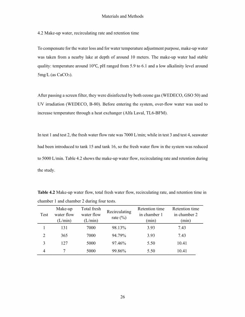
4.2 Make-up water, recirculating rate and retention time ................................................................. 26

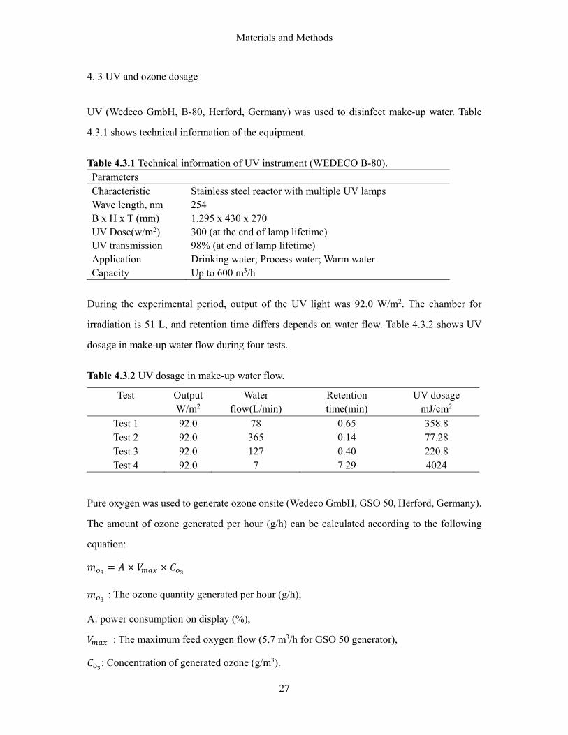
4. 3 UV and ozone dosage ................................................................................................................ 27

4. 4 Analysis of water quality ........................................................................................................... 29

4.4.1Measurement of dissolved oxygen, temperature, pH ............................................................ 29

4.4.2 Measurement of NH4-N, NO2-N, NO3-N and COD .............................................................. 29

4.4.3 Measurement of Alkalinity ................................................................................................... 30

4.4.4 Measurement of total suspended solids (TSS) and turbidity ................................................ 31

viii

4.4.5 Measurement of heterotrophic bacteria load ....................................................................... 31

4.5 Statistical model .......................................................................................................................... 31

4.5.1 Calculation of TAN concentration from NH4-N concentration ............................................ 32

4.5.2 Calculation of areal TAN removal (ATR) rate ..................................................................... 32

4.5.3 Calculation of areal nitrite removal (ANR) rate .................................................................. 32

5. RESULTS ......................................................................................................................................... 33

5.1 Temperature, pH, dissolved oxygen and alkalinity variation in make-up and reused water ...... 33

5.2 Nitrogenous waste concentration and removal rate .................................................................... 33

5.2.1 TAN, free ammonia concentration and Areal TAN Removal (ATR) rate ............................. 33

5.2.2 NO2-N concentration and areal nitrite removal (ANR) rate ................................................ 36

5.2.3 NO3-N concentration variation and relationship with feed loading rate ............................. 38

5.3 COD concentration and removal rate, COD/TAN ratio and TAN reduction (%) ....................... 40

5.3.1 Areal COD removal rate in MBBR ...................................................................................... 40

5.3.2 COD/TAN ration and TAN reduction (%) ........................................................................... 41

5.4 Total Suspended solids (TSS) and its relationship with COD concentration ............................. 43

5.5 Turbidity and its relationship with TSS ...................................................................................... 44

5.6 Heterotrophic bacteria count in make-up water and reused water .............................................. 45

6. DISCUSSION ................................................................................................................................... 47

6.1 The experimental setup ............................................................................................................... 47

6.2 Discussion of water quality and MBBR performance ................................................................ 49

6.2.1 TAN, NO2-N concentration and removal rate ...................................................................... 49

6.2.2 NO3-N variation and feed loading rate ................................................................................ 51

6.2.3 COD variation and COD/TAN ratio .................................................................................... 51

6.2.4 TSS variation ........................................................................................................................ 52

6.3 Function of the closed ozone cabin ............................................................................................. 53

6.4 Heterotrophic bacteria count and disinfection efficiency ........................................................... 54

6.5 Turbidity as a proxy for total suspended solids (TSS) ................................................................ 55

6.6 Future studies .............................................................................................................................. 55

7. CONCLUSION ................................................................................................................................. 56

8. REFERENCES ................................................................................................................................. 57

ix

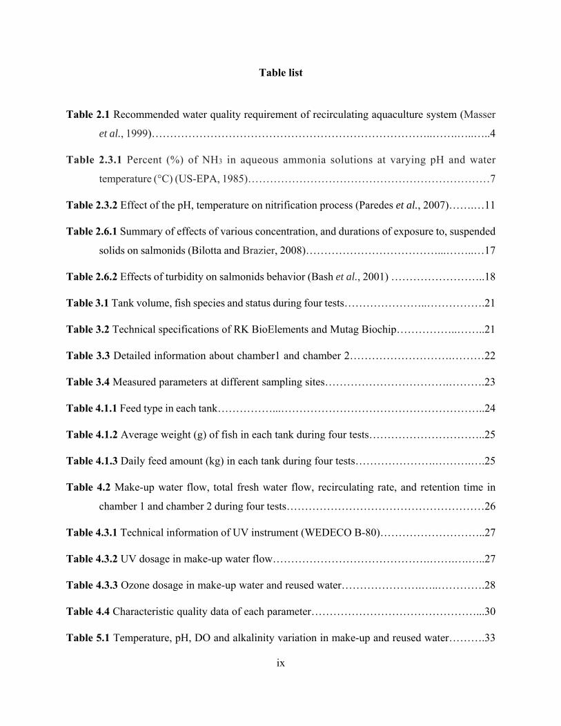
Table list

Table 2.1 Recommended water quality requirement of recirculating aquaculture system (Masser

et al., 1999)…………………………………………………………………..…….…..…..4

Table 2.3.1 Percent (%) of NH3 in aqueous ammonia solutions at varying pH and water

temperature (°C) (US-EPA, 1985)…………………………………………………………7

Table 2.3.2 Effect of the pH, temperature on nitrification process (Paredes et al., 2007)…….…11

Table 2.6.1 Summary of effects of various concentration, and durations of exposure to, suspended

solids on salmonids (Bilotta and Brazier, 2008)………………………………...……..…17

Table 2.6.2 Effects of turbidity on salmonids behavior (Bash et al., 2001) ……………………..18

Table 3.1 Tank volume, fish species and status during four tests…………………..…………….21

Table 3.2 Technical specifications of RK BioElements and Mutag Biochip……………..……..21

Table 3.3 Detailed information about chamber1 and chamber 2……………………….………22

Table 3.4 Measured parameters at different sampling sites…………………………….……….23

Table 4.1.1 Feed type in each tank……………...………………………………………………..24

Table 4.1.2 Average weight (g) of fish in each tank during four tests…………………………..25

Table 4.1.3 Daily feed amount (kg) in each tank during four tests………………….……….….25

Table 4.2 Make-up water flow, total fresh water flow, recirculating rate, and retention time in

chamber 1 and chamber 2 during four tests………………………………………………26

Table 4.3.1 Technical information of UV instrument (WEDECO B-80)………………………..27

Table 4.3.2 UV dosage in make-up water flow…………………………………….…….….…..27

Table 4.3.3 Ozone dosage in make-up water and reused water………………….…..………….28

Table 4.4 Characteristic quality data of each parameter………………………………………...30

Table 5.1 Temperature, pH, DO and alkalinity variation in make-up and reused water……….33

x

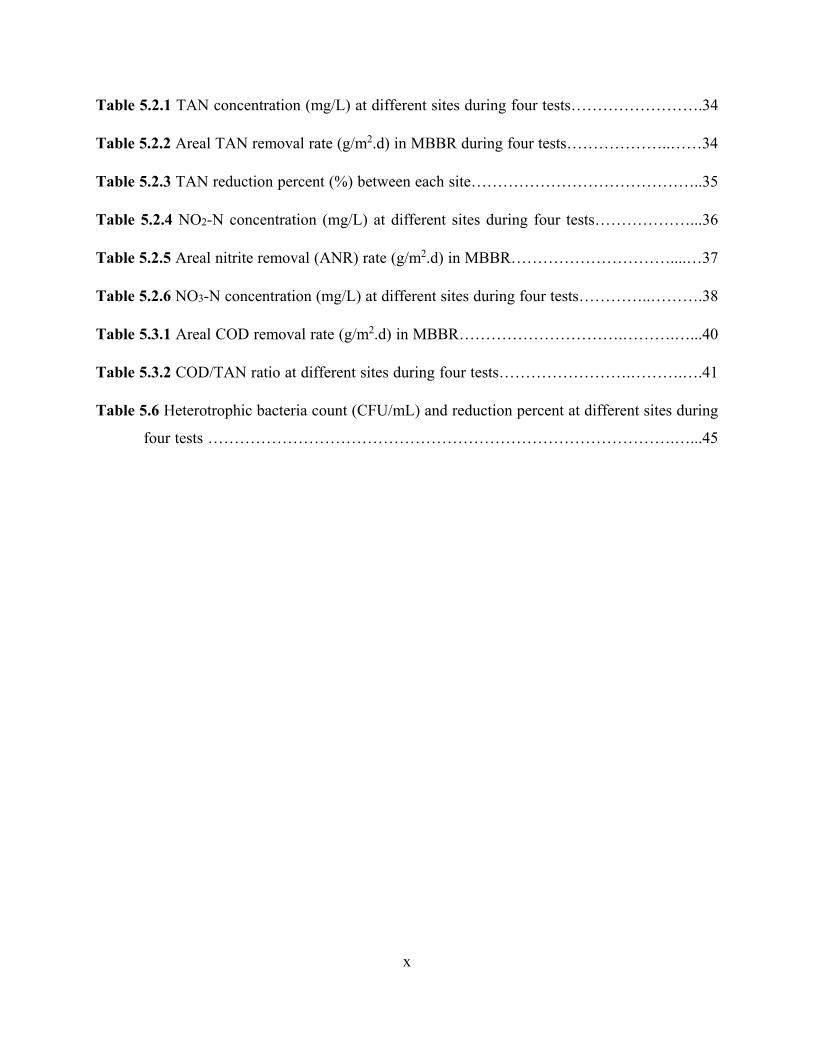
Table 5.2.1 TAN concentration (mg/L) at different sites during four tests…………………….34

Table 5.2.2 Areal TAN removal rate (g/m2.d) in MBBR during four tests………………..……34

Table 5.2.3 TAN reduction percent (%) between each site……………………………………..35

Table 5.2.4 NO2-N concentration (mg/L) at different sites during four tests………………...36

Table 5.2.5 Areal nitrite removal (ANR) rate (g/m2.d) in MBBR…………………………....…37

Table 5.2.6 NO3-N concentration (mg/L) at different sites during four tests…………..……….38

Table 5.3.1 Areal COD removal rate (g/m2.d) in MBBR………………………….……….…...40

Table 5.3.2 COD/TAN ratio at different sites during four tests…………………….……….….41

Table 5.6 Heterotrophic bacteria count (CFU/mL) and reduction percent at different sites during

four tests …………………………………………………………………………….…...45

xi

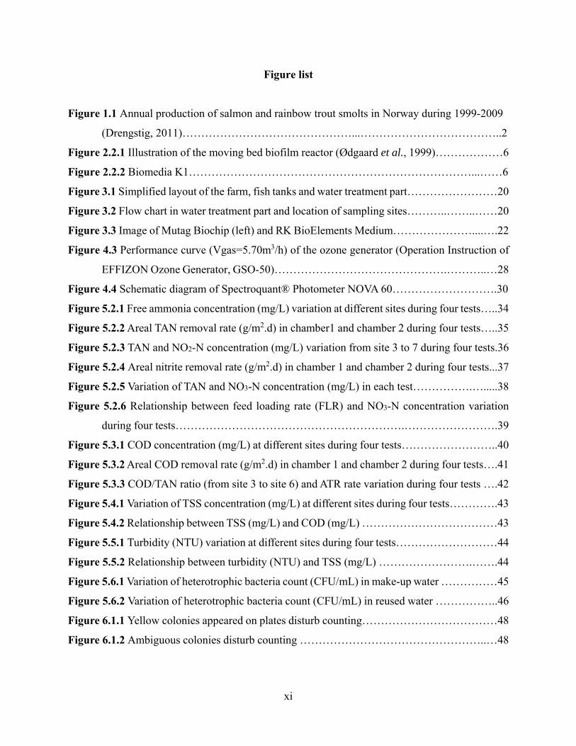
Figure list

Figure 1.1 Annual production of salmon and rainbow trout smolts in Norway during 1999-2009

(Drengstig, 2011)………………………………………...………………………………..2

Figure 2.2.1 Illustration of the moving bed biofilm reactor (Ødgaard et al., 1999)………………6

Figure 2.2.2 Biomedia K1…………………………………………………………………...……6

Figure 3.1 Simplified layout of the farm, fish tanks and water treatment part……………………20

Figure 3.2 Flow chart in water treatment part and location of sampling sites………..……..……20

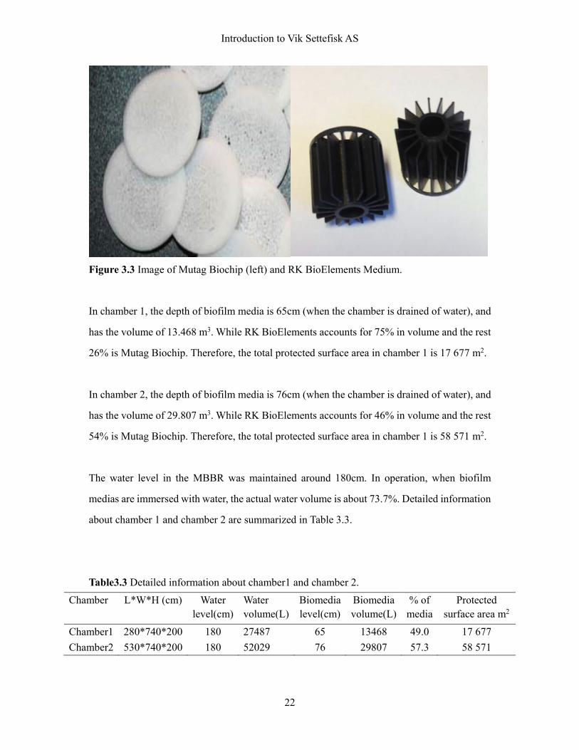
Figure 3.3 Image of Mutag Biochip (left) and RK BioElements Medium…………………....….22

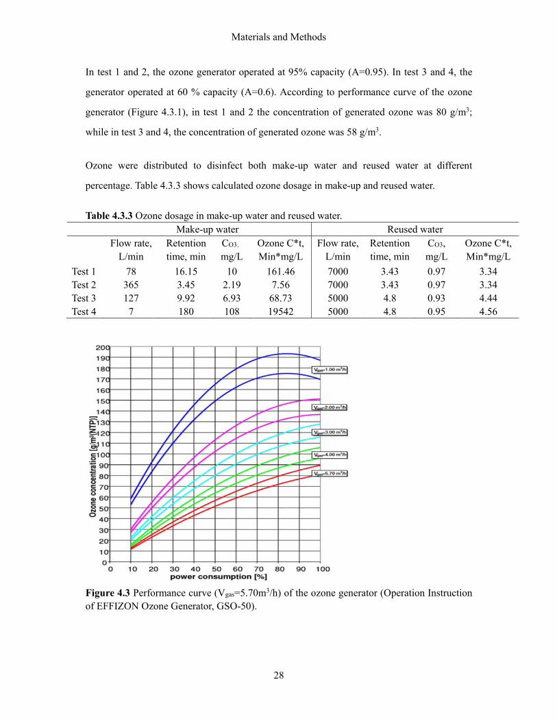
Figure 4.3 Performance curve (Vgas=5.70m3/h) of the ozone generator (Operation Instruction of

EFFIZON Ozone Generator, GSO-50)……………………………………….………..…28

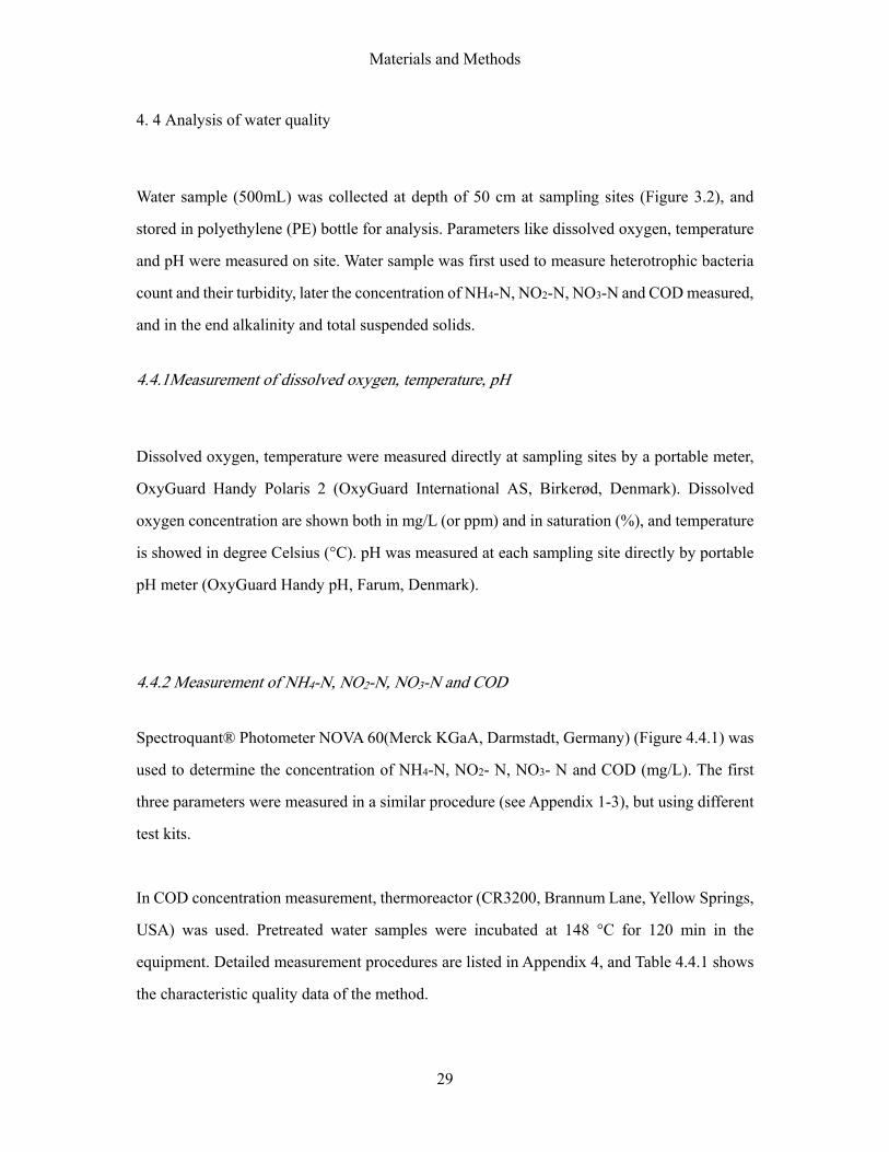
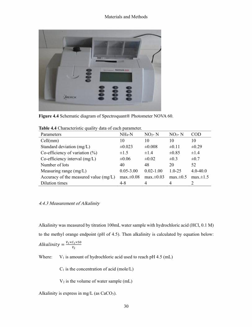
Figure 4.4 Schematic diagram of Spectroquant® Photometer NOVA 60……………………….30

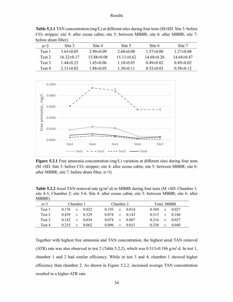
Figure 5.2.1 Free ammonia concentration (mg/L) variation at different sites during four tests…..34

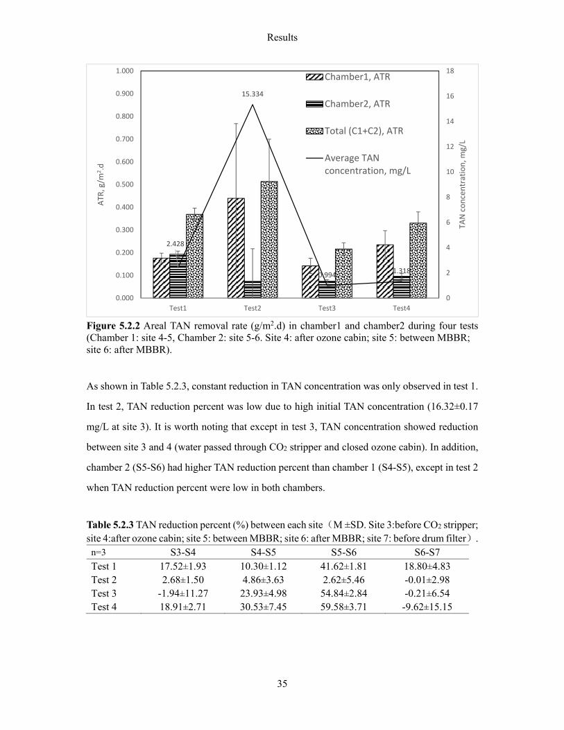
Figure 5.2.2 Areal TAN removal rate (g/m2.d) in chamber1 and chamber 2 during four tests…..35

Figure 5.2.3 TAN and NO2-N concentration (mg/L) variation from site 3 to 7 during four tests.36

Figure 5.2.4 Areal nitrite removal rate (g/m2.d) in chamber 1 and chamber 2 during four tests...37

Figure 5.2.5 Variation of TAN and NO3-N concentration (mg/L) in each test…………….….....38

Figure 5.2.6 Relationship between feed loading rate (FLR) and NO3-N concentration variation

during four tests…………………………………………………….…………………….39

Figure 5.3.1 COD concentration (mg/L) at different sites during four tests……………………..40

Figure 5.3.2 Areal COD removal rate (g/m2.d) in chamber 1 and chamber 2 during four tests….41

Figure 5.3.3 COD/TAN ratio (from site 3 to site 6) and ATR rate variation during four tests ….42

Figure 5.4.1 Variation of TSS concentration (mg/L) at different sites during four tests………….43

Figure 5.4.2 Relationship between TSS (mg/L) and COD (mg/L) ………………………………43

Figure 5.5.1 Turbidity (NTU) variation at different sites during four tests………………………44

Figure 5.5.2 Relationship between turbidity (NTU) and TSS (mg/L) …………………….…….44

Figure 5.6.1 Variation of heterotrophic bacteria count (CFU/mL) in make-up water ……………45

Figure 5.6.2 Variation of heterotrophic bacteria count (CFU/mL) in reused water ……………..46

Figure 6.1.1 Yellow colonies appeared on plates disturb counting………………………………48

Figure 6.1.2 Ambiguous colonies disturb counting …………………………………………..…48

Introduction

1

1. INTRODUCTION

Aquaculture is the farming of aquatic organisms such as fish, crustaceans, molluscs

and aquatic plants, the worldwide demand for fish has provided impetus to rapid growth in

aquaculture (Timmons et al., 2002). In 2012, there were 66.6 million tons of fish produced by

aquaculture, it accounted for 42.2% of world food fish production. In addition, aquaculture is

one of the fastest growing food-producing sectors, with averaged 6.5 % growth in the period

from 2000 to 2012 (FAO, 2014). Aquaculture systems can be classified into three main categories: extensive, semi-intensive and

intensive, based on production per unit volume (m3) or unit area (m2) (Lekang, 2008). Natural

small lakes fall in typical extensive systems, pond culture with feeding or aeration in semi-

intensive, and recirculating aquaculture systems are in intensive. Recirculating aquaculture systems (RAS) are tank-based systems in which environmental

parameters are totally controlled, so fish can be stocked at high density. RAS technology has

been developed and refined for the last three decades (Molleda et al., 2007). RAS technology

has capability to work at high capacity with less water and area requirement as compared with

traditional fish farming, also RAS can reduces chemical and antibiotic usage and waste disposal;

in addition, RAS is species-adaptable, this means fish can be produced year-round (Helfrich

and Libey,1991; Masser et al., 1999; Timmons et al., 2002) . However, RAS needs high capital

and operational investment that is the main demerit. Moreover, it is a complex system for

startup and expertise is needed to maintain and monitor. (Masser et al., 1999).

Water quality control in RAS achieved by many different components. In general, RAS

consists of heater or heat exchanger to adjust water temperature, aeration system to reduce

dissolved CO2 concentration, oxygenation system to supply sufficient oxygen, drum filters to

remove suspended solids, disinfection system (UV and ozone equipment) to inactivate

pathogens and bio filter system to remove nitrogen waste. Alkalinity in the system is controlled

by adding chemicals into it (Ding, 2012).

Introduction

2

By FAO report (2014), it has been observed that farming of salmon and rainbow trout has

developed into a major business in the Norwegian coast. Norway produces nearly 1 million

tons of salmon annually, and the industry aims to produce 2.5 million tons salmon within the

next decade (Drengstig, 2011).

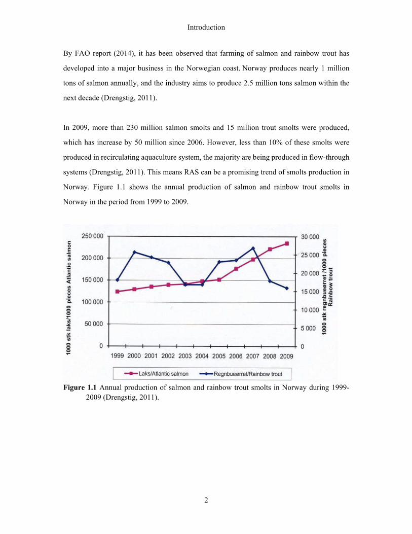
In 2009, more than 230 million salmon smolts and 15 million trout smolts were produced,

which has increase by 50 million since 2006. However, less than 10% of these smolts were

produced in recirculating aquaculture system, the majority are being produced in flow-through

systems (Drengstig, 2011). This means RAS can be a promising trend of smolts production in

Norway. Figure 1.1 shows the annual production of salmon and rainbow trout smolts in

Norway in the period from 1999 to 2009.

Figure 1.1 Annual production of salmon and rainbow trout smolts in Norway during 1999-

2009 (Drengstig, 2011).

Introduction

3

1.1 Objective

To determine water quality variation in a commercial smolts farm employing recirculating

aquaculture system and how is water quality being reconditioned in order to be reused,

To study the nitrification efficiency in moving bed biofilm reactor (MBBR) and changes

in suspended solids and turbidity during the treatment,

To study disinfection efficiency of ozonation and UV irradiation on make-up water, and

disinfection efficiency of ozonation on reused water,

To evaluate whether turbidity could produce a satisfactory estimate of total suspended

solids at Vik Settefisk AS.

Literature Review

4

2. LITERATURE REVIEW

2.1 Water quality in RAS and water quality requirement for salmonids

Optimal and stable water quality is one of the most important factors to successful aquaculture.

One of the major advantages of RAS is the ability to control environment factors and optimize

water quality (Timmons et al., 2002). The critical and decisive parameters of water quality in

aquaculture are: temperature, pH, alkalinity, dissolved oxygen, carbon dioxide, ammonia,

nitrite and suspended solids (Colt, 2006). Depending on farmed species, life stage and farming conditions, different water quality criteria

will be used (Colt, 2006). Table 2.1 shows the recommended water quality requirement of

recirculating aquaculture system (Masser et al., 1999). For salmonids, based on gill damage caused by ammonia exposure, the recommended un-

ionized ammonia criterion in salmonid culture is only 0.0125 mg/L (Westers, 1981). The

optimal temperature for rainbow trout is 14-16 , while for Atlantic salmon is 15 (Aston et

al., 1982). Fivelstad et al. (2003) found increased incidences of nephrocalcinosis when salmon

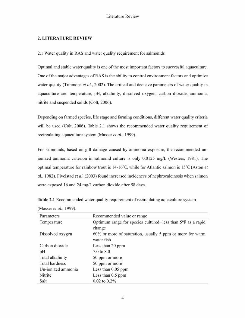
were exposed 16 and 24 mg/L carbon dioxide after 58 days. Table 2.1 Recommended water quality requirement of recirculating aquaculture system

(Masser et al., 1999).

Parameters Recommended value or range Temperature Optimum range for species cultured__less than 5 as a rapid

change Dissolved oxygen 60% or more of saturation, usually 5 ppm or more for warm

water fish Carbon dioxide Less than 20 ppm pH 7.0 to 8.0 Total alkalinity 50 ppm or more Total hardness 50 ppm or more Un-ionized ammonia Less than 0.05 ppm Nitrite Less than 0.5 ppm Salt 0.02 to 0.2%

Literature Review

5

2.2 Description of Moving Bed Biofilm Reactor (MBBR)

There are many types of biofilm systems used for water treatment, such as trickling biofilters,

rotating biological contactors (RBC), granular media biofilters, floating bead biofilters and

fluidized bed biofilters (Timmons et al., 2002), they all have advantages and disadvantages.

The trickling filter is not volume-effective; mechanical failures have often been experienced in

rotating biological contactors; granular media biofilters need periodic back flashing and the

fluidized bed reactors show hydraulic instability (Rusten et al., 2006). In this context, the

moving bed biofilm reactor (MBBR) technology was developed in the late 1980s and early

1990s in Norway (Ødgaard et al., 1999).

Now MBBR has been applied world-widely for treatment of municipal and industrial

wastewaters, as well as for water treatment in aquaculture (Rusten et al., 2006). In aquaculture

industry, MBBR is mainly applied for nitrification, as well as removal of organic matters. In

order to avoid the heterotrophic bacteria that consume organic matters suppressing the

nitrifying bacteria at high organic loads, MBBR is always operated at low organic loads in

aquaculture system (Rusten et al., 2006).

Compared with most other biofilm reactors, MBBR utilizes the whole tank volume for biomass

growth, it also has an insignificant head-loss and no need for periodic backwashing and not

susceptible for clogging (Rusten et al., 2006). In addition, the filling fraction of biofilm carriers

in the reactor can be subject to preferences. However, it is recommended that filling fractions

should be less than 70 % to keep the carrier suspended freely in reactor (Ding, 2012).

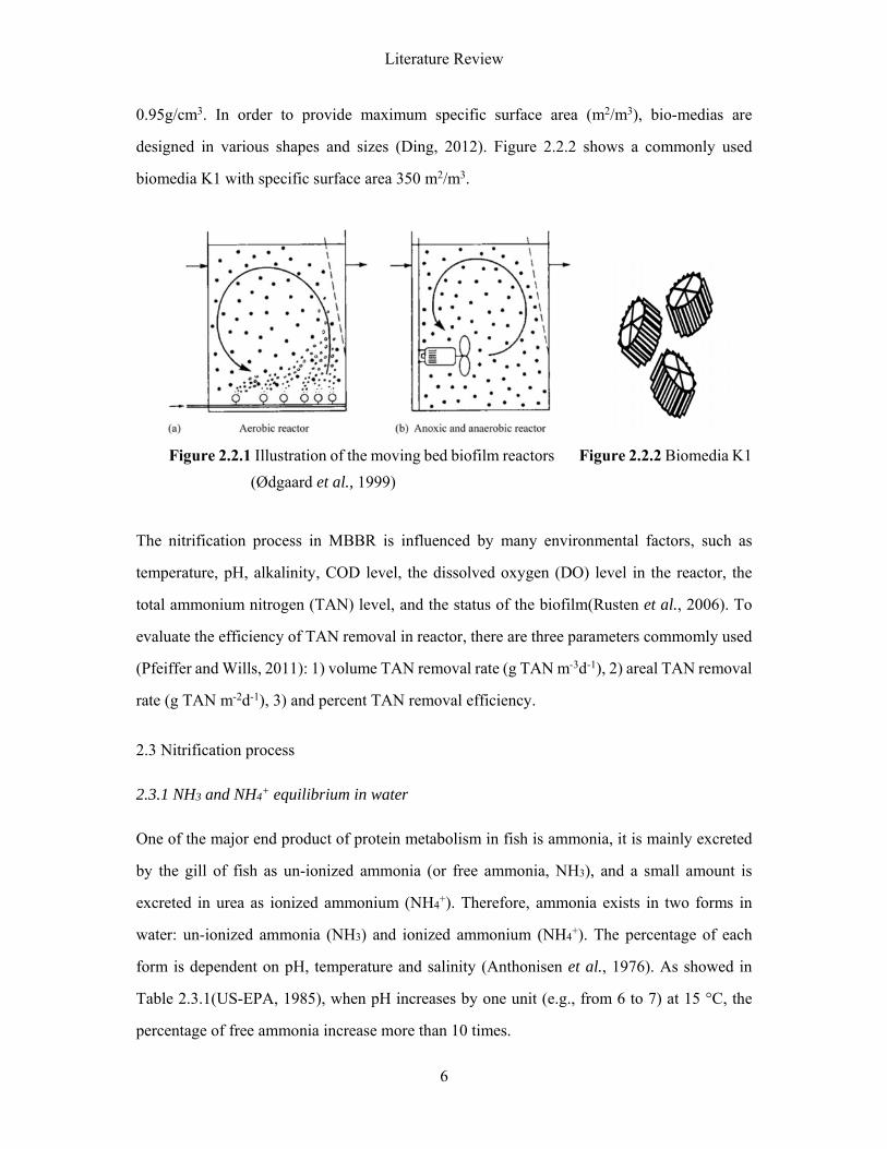
MBBR is a technology based on biofilm theory, with an active biofilm growing on specially

designed plastic carriers (or biomedia) that are suspended in the reactor. It can be operated both

in aerobic and anaerobic conditions, as illustrated in Figure 2.2.1. In aerobic case, the biomedia

are kept suspended by agitation from aeration diffusers, while in anaerobic case, a mixer is

used to keep the biomedia moving (Ødgaard et al., 1999). Bio-medias are made from different

materials and high-density polyethylene is commonly used, which has a density about

Literature Review

6

0.95g/cm3. In order to provide maximum specific surface area (m2/m3), bio-medias are

designed in various shapes and sizes (Ding, 2012). Figure 2.2.2 shows a commonly used

biomedia K1 with specific surface area 350 m2/m3.

Figure 2.2.1 Illustration of the moving bed biofilm reactors Figure 2.2.2 Biomedia K1

(Ødgaard et al., 1999)

The nitrification process in MBBR is influenced by many environmental factors, such as

temperature, pH, alkalinity, COD level, the dissolved oxygen (DO) level in the reactor, the

total ammonium nitrogen (TAN) level, and the status of the biofilm(Rusten et al., 2006). To

evaluate the efficiency of TAN removal in reactor, there are three parameters commomly used

(Pfeiffer and Wills, 2011): 1) volume TAN removal rate (g TAN m-3d-1), 2) areal TAN removal

rate (g TAN m-2d-1), 3) and percent TAN removal efficiency.

2.3 Nitrification process

2.3.1 NH3 and NH4+ equilibrium in water

One of the major end product of protein metabolism in fish is ammonia, it is mainly excreted

by the gill of fish as un-ionized ammonia (or free ammonia, NH3), and a small amount is

excreted in urea as ionized ammonium (NH4+). Therefore, ammonia exists in two forms in

water: un-ionized ammonia (NH3) and ionized ammonium (NH4+). The percentage of each

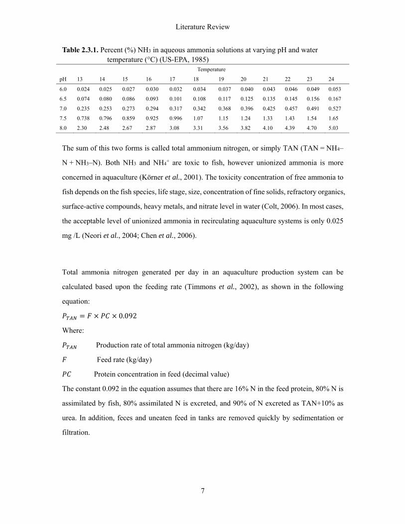
form is dependent on pH, temperature and salinity (Anthonisen et al., 1976). As showed in

Table 2.3.1(US-EPA, 1985), when pH increases by one unit (e.g., from 6 to 7) at 15 °C, the

percentage of free ammonia increase more than 10 times.

Literature Review

7

Table 2.3.1. Percent (%) NH3 in aqueous ammonia solutions at varying pH and water temperature (°C) (US-EPA, 1985)

Temperature

pH 13 14 15 16 17 18 19 20 21 22 23 24

6.0 0.024 0.025 0.027 0.030 0.032 0.034 0.037 0.040 0.043 0.046 0.049 0.053

6.5 0.074 0.080 0.086 0.093 0.101 0.108 0.117 0.125 0.135 0.145 0.156 0.167

7.0 0.235 0.253 0.273 0.294 0.317 0.342 0.368 0.396 0.425 0.457 0.491 0.527

7.5 0.738 0.796 0.859 0.925 0.996 1.07 1.15 1.24 1.33 1.43 1.54 1.65

8.0 2.30 2.48 2.67 2.87 3.08 3.31 3.56 3.82 4.10 4.39 4.70 5.03

The sum of this two forms is called total ammonium nitrogen, or simply TAN (TAN = NH4–

N + NH3–N). Both NH3 and NH4+ are toxic to fish, however unionized ammonia is more

concerned in aquaculture (Körner et al., 2001). The toxicity concentration of free ammonia to

fish depends on the fish species, life stage, size, concentration of fine solids, refractory organics,

surface-active compounds, heavy metals, and nitrate level in water (Colt, 2006). In most cases,

the acceptable level of unionized ammonia in recirculating aquaculture systems is only 0.025

mg /L (Neori et al., 2004; Chen et al., 2006).

Total ammonia nitrogen generated per day in an aquaculture production system can be

calculated based upon the feeding rate (Timmons et al., 2002), as shown in the following

equation:

0.092

Where:

Production rate of total ammonia nitrogen (kg/day)

Feed rate (kg/day)

Protein concentration in feed (decimal value)

The constant 0.092 in the equation assumes that there are 16% N in the feed protein, 80% N is

assimilated by fish, 80% assimilated N is excreted, and 90% of N excreted as TAN+10% as

urea. In addition, feces and uneaten feed in tanks are removed quickly by sedimentation or

filtration.

Literature Review

8

2.3.2 Nitrification process description

Nitrification is an important process in the cycling of nitrogen. There are three nitrogen

conversion pathways that normally existed in aquaculture systems for the removal of

ammonia–nitrogen. They are:

*Photoautotrophic removal by algae;

*Autotrophic bacterial conversion of ammonia–nitrogen to nitrate–nitrogen;

*Heterotrophic bacterial conversion of ammonia–nitrogen to microbial biomass.

The nitrification process is carried out by nitrifying bacteria and it has been well studied,

nitrifying bacteria are chemoautotrophic and they get energy for life process from nitrification

reaction (Barnes and Bliss, 1983; Wiesmann, 1994).

First free ammonia is oxidized to nitrite by ammonia oxidizing bacteria genera (such as

Nitrosomonas, Nitrosospira, and Nitrosococcus), as shown in Equation 2.1. Then nitrite is

oxidized to less toxic nitrate by nitrite oxidizing bacteria genera (such as Nitrobacter and

Nitrospira), as showed in Equation 2.2. These reactions will consume oxygen and produce

hydrogen ions (which would result in decline of pH).

NH4+ + 1.5O2 → NO2− + H2O + 2H+………………….…………………….....….Equation 2.1

NO2− + 0.5O2 → NO3–…………………………………………………………….Equation 2.2

According to US-EPA (1984), the complete nitrification process can be express as:

NH4+ + 1.83O2+1.98HCO3- →0.021C5H7O2N+0.98 NO3–+1.041 H2O+1.88 HCO3-

………………………………………………………………………………….Equation 2.3

Here C5H7O2N presents the chemical composition of nitrifying bacteria. From Equation 2.3,

we know that for every gram of TAN being oxidized to nitrate nitrogen, approximately 4.18 g

of oxygen and 7.07 g of alkalinity (as CaCO3) are consumed and 0.17 g nitrifying bacteria

biomass are produced (Chen et al., 2006).

Literature Review

9

Heterotrophic bacterial also present in water, their growth will be stimulated at high

concentration of organic substrate. At high carbon to nitrogen(C/N) feed ratio, heterotrophic

bacteria can also assimilate ammonia-nitrogen directly into cellular protein (Ebeling et al.,

2006). Lipponen et al. (2004) and Summerfelt et al. (2004) reported that heterotrophic bacteria

could assimilate the ammonia and participate in the process of biofilm building, by utilizing

soluble organic carbon.

2.3.3 Effect of alkalinity on nitrification rate

As shown in Equation 2.3, HCO3- is being consumed in nitrification process constantly. For

every kilogram of feed consumed by fish, approximately 0.15–0.19 kg sodium bicarbonate

(NaHCO3) needs to be added into water (Davidson et al., 2011). If the alkalinity loss is not

compensated by supplementation with a base (such as sodium hydroxide or sodium

bicarbonate), the alkalinity and pH of the system will decrease gradually (Loyless and Malone,

1997).

In addition, Paz (2000) and Biesterfeld et al. (2003) found that maintaining adequate alkalinity

concentrations is critical for sustainable nitrification. In a bench-scale experiment performed

in a turbot farm using moving bed biological reactor(MBBR), Rusten et al. (2006) found that

the nitrification rate dropped to only half of the original rate when alkalinity dropped from

approximately 115 mg/L as CaCO3(pH=7.3) to 57 mg/L (pH=6.7). Villaverde et al. (1997)

reported a linear increase in nitrification efficiency of 13% per unit pH increase from pH 5.0

to 8.5.

Mydland et al. (2010) reported that if recirculating aquaculture system was operated with sub

optimal alkalinity, theoretically it could encounter larger pH fluctuation, higher concentrations

of TAN and NO2–N due to accumulation, and microbial community instability, which is

harmful to the fish. Especially for Atlantic salmon, which is sensitive to elevated concentrations

of nitrite nitrogen without concurrent chloride adjustments (Gutierrez et al., 2011).

Literature Review

10

2.3.4 Effect of C/N ratio on nitrification rate

At a high C/N ratios, the heterotrophic bacteria out-compete nitrifying bacteria (autotrophic)

for available oxygen and space in the biofilters (Michaud et al., 2006). One of the critical

factors affecting the design and operation of a nitrification system is the ratio of the

biodegradable organic carbon to the nitrogen, or C/N ratio (US-EPA, 1993). As previously

mentioned in Section 2.3.2, there are three pathways in nitrogen cycle and two genres of

bacteria are involved in nitrification. Autotrophic bacteria derive their energy from inorganic

compounds and heterotrophic bacteria that derive energy from organic compounds (Hagopian

and Riley, 1998). Actually, heterotrophic bacteria have a maximum growth rate significantly

higher than nitrifying bacteria (US-EPA, 1993). Therefore, nitrification prefer a low C/N ratio.

2.3.5 Effect of PH on nitrification rate

Many authors have reported that the optimum pH range for nitrification is from 7.0 to 8.0

(Jones and Paskins, 1982; Painter and Loveless, 1983; Antoniou et al., 1990). As showed in

Table 2.3.2, the optimum pH range for Nitrosomonas is 7.9 - 8.2, and 7.2 – 7.6 for Nitrobacter

(Alleman, 1984). pH influences nitrifying bacteria in three ways. First is the activation - deactivation of nitrifying

bacteria. The change of pH will lead to binding of H+ or OH- ions with the weak basic-acid

groups and then blocking the active sites of nitrifying bacteria on biofilms (Quinlan, 1984).

Second is the influence on availability of mineral carbon nutritional, which is the carbon source

for nitrifying autotrophic bacteria. Availability of carbon source is also related to alkalinity.

However, pH plays an important role in carbon equilibrium.

The third effect is inhibition of free ammonia and free nitrous acid (Anthonisen et al., 1976;

Ford et al., 1980), and heavy metals (Braam and Klapwijk, 1981; Nelson et al., 1981).

Concentrations of free ammonia and nitrous acid depends on temperature, pH, and the

Literature Review

11

concentrations ammonium and nitrite. Free ammonia concentration increases at high pH,

whereas nitrous acid concentrations rises at low pH (Ford et al., 1980).

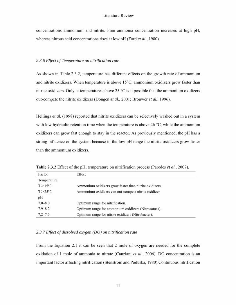
2.3.6 Effect of Temperature on nitrification rate

As shown in Table 2.3.2, temperature has different effects on the growth rate of ammonium

and nitrite oxidizers. When temperature is above 15°C, ammonium oxidizers grow faster than

nitrite oxidizers. Only at temperatures above 25 °C is it possible that the ammonium oxidizers

out-compete the nitrite oxidizers (Dongen et al., 2001; Brouwer et al., 1996).

Hellinga et al. (1998) reported that nitrite oxidizers can be selectively washed out in a system

with low hydraulic retention time when the temperature is above 26 °C, while the ammonium

oxidizers can grow fast enough to stay in the reactor. As previously mentioned, the pH has a

strong influence on the system because in the low pH range the nitrite oxidizers grow faster

than the ammonium oxidizers.

Table 2.3.2 Effect of the pH, temperature on nitrification process (Paredes et al., 2007). Factor Effect Temperature T＞15 Ammonium oxidizers grow faster than nitrite oxidizers. T＞25 Ammonium oxidizers can out-compete nitrite oxidizer. pH 7.0–8.0 Optimum range for nitrification. 7.9–8.2 Optimum range for ammonium oxidizers (Nitrosomas). 7.2–7.6 Optimum range for nitrite oxidizers (Nitrobacter).

2.3.7 Effect of dissolved oxygen (DO) on nitrification rate

From the Equation 2.1 it can be seen that 2 mole of oxygen are needed for the complete

oxidation of 1 mole of ammonia to nitrate (Canziani et al., 2006). DO concentration is an

important factor affecting nitrification (Stenstrom and Poduska, 1980).Continuous nitrification

Literature Review

12

under low DO will leads to nitrite accumulation, because nitrite oxidizers is more sensitive to

oxygen than ammonia oxidizers (Jayamohan et al., 1988).

Dissolved oxygen concentration is also an important factor and it is related to the thickness of

the biofilm and temperature (Haoa et al., 2002). With a defined ammonium surface load (ASL)

under lower temperature, a thicker biofilm is required and, hence, a higher dissolved oxygen

concentration is necessary in the reactor. A thin biofilm needs a lower dissolved oxygen

concentration. Higher dissolved oxygen concentrations will cause total nitrification and a lower

nitrogen removal rate (Koch et al., 2000; Haob et al., 2002).

2.4 Disinfection by ozonation and UV irradiation

Ozone is a powerful oxidant which has been widely applied in RAS, especially within recently

constructed intensive salmonid production systems (Summerfelt et al., 2001). Ozone is added

into aquaculture system waters for both disinfection and water quality improvement purposes

(Wedemeyer, 1996). It works well in fish pathogens inactivation, organic wastes removal

(including color and smell removal) and nitrite oxidization. Besides, ozonation of water in

recirculating systems improves fish welfare by reducing fish disease and environmental sources

of stress (Brazil, 1996).

At 20 , the half-life of ozone dissolved in pure water is 165 min (Rice et al., 1981). In

recirculating aquaculture systems, where reused water contains high levels of organic material

and nitrogen waste, will leads to an even shorter half-life time (e.g., <15 s), which makes

maintaining a specific concentration of ozone residual difficult (Bullock et al., 1997),

therefore it has to be produced and used on site.

Literature Review

13

Ozone is generally produced by leading enriched oxygen feed gas through a high-voltage

electrical corona. Pure oxygen is mostly being used because it is not only 2-3 times more

energy-efficient when compared with using air (Masschelein, 1998), but also pure oxygen gas

is often already used to maximize carrying capacity in most intensive fish farms. All typical

oxygen transferring devices can be used to transfer ozone gas to water as well (Summerfelt and

Hochheimer, 1997). Continuous liquid-phase transfer units are usually selected when the ozone

residual must be kept for a certain time (Bellamy et al., 1991). High column bubble diffusers

are frequently used in fish farms and in this way more than 85% of ozone are transfer to the

liquid phase (Liltved, 2001).

Ozonation can kill bacteria, virus and other microorganisms in water, but to get an ideal

disinfection effect it requires keeping a certain dissolved ozone level for a given contact

time(c*t effect). Literature reviews on ozone dosing requirements indicates that many

pathogenic organism can be inactivated by an ozone c*t dosages of 0.5-5.0 min mg/L (Liltved,

2001). However, certain kinds of spore forming organism are difficult to inactivate by ozone.

For this reason, to disinfect water in recirculating aquaculture systems thoroughly, it needs

much greater ozone dosages than it is typically required for simply water quality control

(Bullock et al., 1997). Ozone can also been used to disinfect effluent from hatcheries or farms

in order to prevent the potential release of fish pathogens to the receiving watershed (Liltved,

2001).

Although ozone has a rapid reaction rate and little harmful by-products, it is lethal to fish at a

very low levels which may be as low as 0.01 mg/L, the maximum safe level of chronic ozone

exposure for salmonids is 0.002 mg/L (Wedemeyer et al., 1979). Compilation of results from

several other studies shows that most fish exposed to ozone levels that more than 0.008-0.06

mg/L will develop severe gill damages which can result in serum osmolality imbalances or kill

fish immediately or leave them more susceptible to pathogens (Bullock et al., 1997). To

avoid this problem, ozone residual can be removed by increasing the contact times, aeration

and degassing, reaction with hydrogen peroxide, or intense UV light irradiation.

Literature Review

14

UV irradiation is also widely used in aquaculture industry to inactivate microorganisms

(Sharrer et al., 2005). Compared with ozone, using of UV light will not produce toxic residuals

or form harmful byproducts to fish at all. UV light functions by breaking down the nucleic

acids of microorganisms, which will result in death or function lose. Microorganism can be

inactivated at UV wavelengths ranging from 100 to 400 nm, while 254 nm is the most effective

wavelength. Ozone residuals can also be removed at specific UV wavelength from 250-260nm.

According to Hunter et al. (1998), completely ozone residuals removal can be achieved at UV

doses of 60-75 mW s/cm2, even if the ozone concentration is as high as 0.5 mg/L.

Most fish pathogens can be inactivated by UV doses of 30 mW s/cm2 at 254nm. But according

to required removal rate and targeted pathogens, the UV doses requirement ranges wildly from

2 mW s/cm2 to 230 mW s/cm2 (Wedemeyer, 1996). Actually, the real UV dose requirement

depends largely on UV intensity, exposure time, water flow and transmittance of UV in water.

In order to get better disinfection, exposure time or UV intensity are often increased in practice,

because UV transmittance is conversely reduced with increase in total suspended solids

concentration (Loge et al., 1996) and pathogens may be shield by envelop with particulate

matter (Emerick et al., 1999). Sharrer et al. (2005) presented a hypothesis that in reused

aquaculture system where reused water is treated with UV irradiation may provide selection

pressure for some bacteria species that merged together with particulate matter, because this

provides protection from the UV irradiation.

Ozonation followed by UV irradiation has been applied in wastewater and drinking water

treatment to get best removal of microorganisms for decades (White, 2005). In RAS, if certain

amount of ozone is used to disinfection, it can prevent accumulation of fine particles in the

system, which could subsequently improve the disinfection efficiency of UV irradiation.

Research done by Sharrer and Summerfelt (2007) also indicated ozonation followed by UV

irradiation provides effective bacteria inactivation in a freshwater recirculating system,

combining ozone dosages of only 0.1–0.2 min mg/L with a UV irradiation dosage of

approximately 50 mJ/cm2 would consistently reduce bacteria counts to near zero.

Literature Review

15

To sum up, according to water quality and disinfection goal, attention must be paid when UV

and ozone are used in fish farm, both the amount and contact time. UV plants are cheaper and

less complex compared with ozone plant. In addition, there is no toxic byproduct or residual

problems related with UV irradiation. However, when water is turbid, UV has little disinfection

effect. In this case, ozone will still works well in oxidizing organic particle, removal of color

and smell, as well as disinfection if ozone is abundant in amount. Therefore, ozonation and UV

irradiation are always being used together in water treatment in RAS.

2.5 Oxygenation and carbon dioxide control in RAS

Pure oxygen has been used in aquaculture to intensify fish production since the 1970s (Speece,

1981). Oxygenation applied in intensive fish farming systems can increase the carrying

capacity notably at a given water flow by removing oxygen concentration as the first limiting

factor (Summerfelt et al., 2000). The use of pure oxygen gas can also reduce production costs,

by increasing carrying capacity and reducing water consumption. Since pure oxygen is not inexpensive, oxygenation should be done at a proper way with high

oxygen transfer efficiency and oxygen absorption efficiency. In general, oxygenation

technology has been well developed and there are various equipment that suitable for different

production system, for example, U-tubes, oxygenation cones and multi-staged low head

oxygenators are widely used in recirculating aquaculture system. Oxygen supersaturated water

should be injected to the bottom of fish tanks and be distributed evenly as soon as possible in

the tank (Masser et al., 1999). For every mole oxygen being consumed by fish and bacteria in system, one mole carbon

dioxide is produced. Furthermore, RAS has a relative low water exchange rates (1%-10%), and

systems with oxygenation typically do not allow for the removal of carbon dioxide in large

amount (Grace and Piedrahita, 1994). Therefore, in intensive recirculating aquaculture system

where large amounts of pure oxygen are added into water, carbon dioxide accumulation is a

practical problem (Summerfelt et al., 2003).

Literature Review

16

High level of dissolved carbon dioxide is toxic to fish, elevated CO2 level may decrease the

ability of hemoglobin to transport oxygen (the Bohr effect), even higher level will decrease the

maximum oxygen binding capacity of blood (the Root effect), and increase blood acidity

(Jobling, 1994). Tolerance to dissolved carbon dioxide depends on fish species, life stage of

the fish, and many other environmental factors, such as alkalinity, pH, and dissolved oxygen

levels (Summerfelt et al., 2000). Salmonids will be affected when dissolved carbon dioxide is

approximately 20 mg/L, while tilapia and catfish will tolerate dissolved carbon dioxide levels

up to 60 mg/L (Wedemeyer, 1996).

Since carbon dioxide is much more soluble than oxygen in water, it is essential that CO2

stripping should be done before oxygenation. In practice, packed column aerators with forced

ventilation are widely used, because they are more effective than diffuser aeration and sub-

surface aerators (Colt and Orwicz, 1991). Packed column aerators are filled with packing (e.g.,

plastic balls) that can increase water-air contact surface and contact time. For most effective

carbon dioxide stripping, at least 5-10 vol. air per vol. water should be contacted (Summerfelt

et al., 2000), this can be achieved by installing blower at the bottom of packed column aerator.

2.6 Effects of total suspended solids (TSS) and turbidity on salmonids

The term total suspended solids (TSS) refers to the mass (mg) or concentration (mg/L) of

inorganic and organic matter which is held in the water by turbulence (Bilotta and Brazier,

2008). They are typically consisted of fine particles with a diameter less than 62 μm (Waters,

1995), and are measured directly by collection of sample water followed by filtration of this

sample through a dried and pre-weighed 0.7 µm pore-size glass fiber-filter (Gray et al., 2000) .

Suspended solids can cause water quality deterioration in many ways. Physically, TSS can

result in reduced penetration of light and temperature changes (Ryan, 1991); Chemically,

contaminants may be released due to TSS presence, such as heavy metals and pesticides

(Dawson and Macklin, 1998); furthermore, if TSS have a high organic content, dissolved

Literature Review

17

oxygen will be consumed by in-situ decomposition, which may lead to low dissolved oxygen

concentration and even kills fish (Ryan, 1991).

TSS can also affect the free-living fish directly, by clogging and being abrasive to fish gills

(Cordone and Kelley, 1961), or stressing the fish and destroying their immune system which

will result in increased disease susceptibility and osmotic dysfunction (Redding et al., 1987).

Migration of wild Salmonids can be influenced by TSS presence (Bisson and Bilby, 1982).

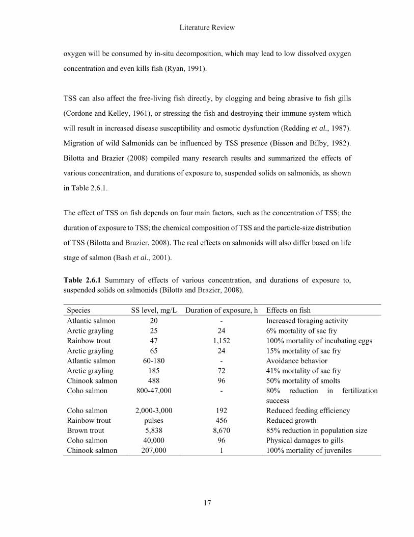
Bilotta and Brazier (2008) compiled many research results and summarized the effects of

various concentration, and durations of exposure to, suspended solids on salmonids, as shown

in Table 2.6.1. The effect of TSS on fish depends on four main factors, such as the concentration of TSS; the

duration of exposure to TSS; the chemical composition of TSS and the particle-size distribution

of TSS (Bilotta and Brazier, 2008). The real effects on salmonids will also differ based on life

stage of salmon (Bash et al., 2001). Table 2.6.1 Summary of effects of various concentration, and durations of exposure to, suspended solids on salmonids (Bilotta and Brazier, 2008). Species SS level, mg/L Duration of exposure, h Effects on fish Atlantic salmon 20 - Increased foraging activity Arctic grayling 25 24 6% mortality of sac fry Rainbow trout 47 1,152 100% mortality of incubating eggs Arctic grayling 65 24 15% mortality of sac fry Atlantic salmon 60-180 - Avoidance behavior Arctic grayling 185 72 41% mortality of sac fry Chinook salmon 488 96 50% mortality of smolts Coho salmon 800-47,000 - 80% reduction in fertilization

success Coho salmon 2,000-3,000 192 Reduced feeding efficiency Rainbow trout pulses 456 Reduced growth Brown trout 5,838 8,670 85% reduction in population size Coho salmon 40,000 96 Physical damages to gills Chinook salmon 207,000 1 100% mortality of juveniles

Literature Review

18

Turbidity is a measurement of light scattering properties of water. Due to low cost and ease of

use, Nephelometric turbidity meters have been most widely applied in field study, and turbidity

data are recorded in nephelometric turbidity units (NTU) (Lewis, 1996).

There are differences and correlations between suspended solids and turbidity. Suspended

solids is the actual measure of the amount of sediment suspended in water column, the process

is complex and time consuming. While turbidity is the measure of the refractory characteristic

of materials in water. So there are many limitations when using turbidity as a surrogate measure

of SS (Bilotta and Brazier, 2008). Because besides concentrations of TSS, turbidity is also

being influenced by the particle-size distribution, shape of particles and other dissolved

materials (Sorenson et al., 1977).

Studies have showed that the turbidity levels beyond natural background can affect the

physiology and behavior of salmonids (Gregory and Northcote, 1993). Exposure to high levels

of suspended solids may be fatal to salmonids, while lower levels of suspended solids and

turbidity will also lead to chronic sub lethal effects such as loss or reduction of foraging

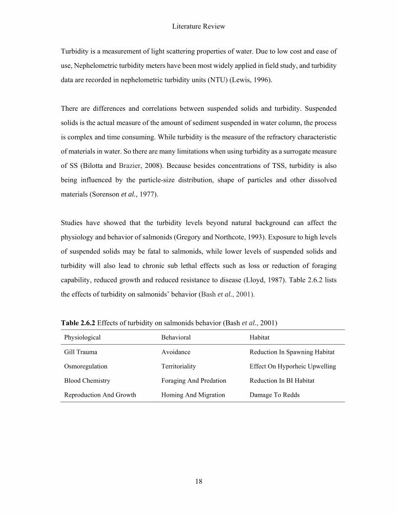
capability, reduced growth and reduced resistance to disease (Lloyd, 1987). Table 2.6.2 lists

the effects of turbidity on salmonids’ behavior (Bash et al., 2001).

Table 2.6.2 Effects of turbidity on salmonids behavior (Bash et al., 2001)

Physiological Behavioral Habitat

Gill Trauma Avoidance Reduction In Spawning Habitat

Osmoregulation Territoriality Effect On Hyporheic Upwelling

Blood Chemistry Foraging And Predation Reduction In BI Habitat

Reproduction And Growth Homing And Migration Damage To Redds

Introduction to Vik Settefisk AS

19

3. INTRODUCTION TO VIK SETTEFISK AS

3.1 Site location, water source and history

The two-month (July to august in 2014) case study was conducted at Vik Settefisk AS, a smolts

farm was located in the western coast of Bergen, Norway. It is a land-based farm established

in 1978, it has abundant fresh water resource from a nearby lake and it is close to sea. Salmon

and rainbow trout fry in the farm were bought from Strømsnes Akvakultur AS and AquaGen

AS respectively.

After many years’ success since establishment, the farm suffered from water quality problem

from 2008 to 2012. RAS was introduced to Vik Settefisk AS in December of 2012. Before that

the main water treatment was total suspended solids removal, and production capacity was

limited with many uncertainties. After employing RAS, water quality became better and more

stable, in consequence the production of salmon smolts had doubled between 2011and 2013,

which increased from 255 000 to 570 000.

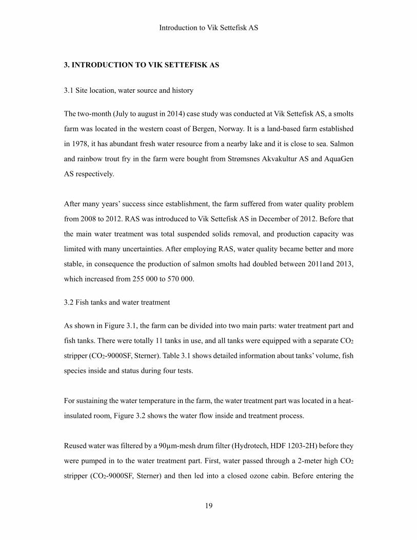
3.2 Fish tanks and water treatment

As shown in Figure 3.1, the farm can be divided into two main parts: water treatment part and

fish tanks. There were totally 11 tanks in use, and all tanks were equipped with a separate CO2

stripper (CO2-9000SF, Sterner). Table 3.1 shows detailed information about tanks’ volume, fish

species inside and status during four tests.

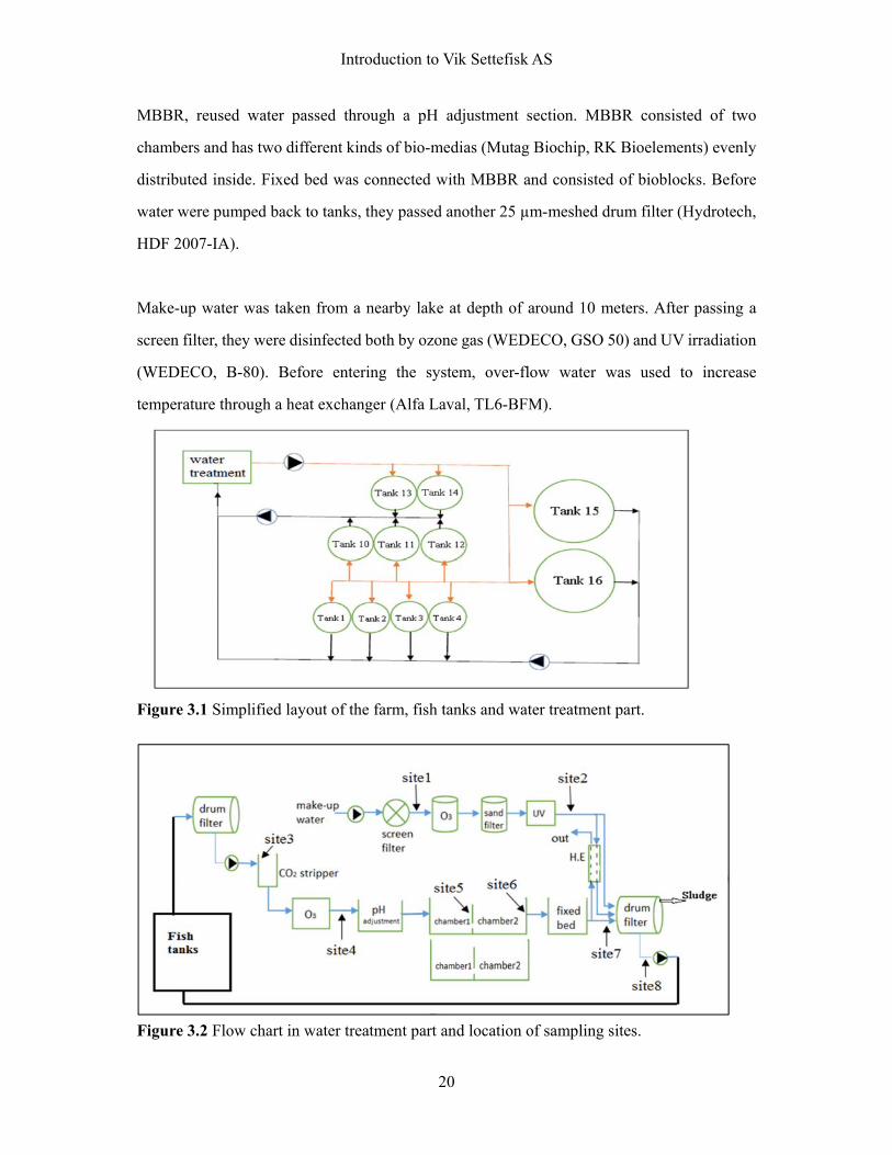
For sustaining the water temperature in the farm, the water treatment part was located in a heat-

insulated room, Figure 3.2 shows the water flow inside and treatment process.

Reused water was filtered by a 90µm-mesh drum filter (Hydrotech, HDF 1203-2H) before they

were pumped in to the water treatment part. First, water passed through a 2-meter high CO2

stripper (CO2-9000SF, Sterner) and then led into a closed ozone cabin. Before entering the


20

MBBR, reused water passed through a pH adjustment section. MBBR consisted of two

chambers and has two different kinds of bio-medias (Mutag Biochip, RK Bioelements) evenly

distributed inside. Fixed bed was connected with MBBR and consisted of bioblocks. Before

water were pumped back to tanks, they passed another 25 µm-meshed drum filter (Hydrotech,

HDF 2007-IA).

Make-up water was taken from a nearby lake at depth of around 10 meters. After passing a

screen filter, they were disinfected both by ozone gas (WEDECO, GSO 50) and UV irradiation

(WEDECO, B-80). Before entering the system, over-flow water was used to increase

temperature through a heat exchanger (Alfa Laval, TL6-BFM).

Figure 3.1 Simplified layout of the farm, fish tanks and water treatment part.

Figure 3.2 Flow chart in water treatment part and location of sampling sites.


21

Table 3.1 Tank volume, fish species and status during four tests. Tank No.

Tank volume (m3)

Indoors or outdoors

Species Test 1 (990m3)

Test 2 (1020m3)

Test 3 (420m3)

Test 4 (420m3)

1 30 Outdoors Fry (Salmon) √ √ √ √



4 30 Outdoors Fry (Salmon) N √ √ √

10 60 Indoors Fry (Salmon) √ √ √ √

11 60 Indoors Fry (Rainbow trout) √ √ √ √




15 300 Outdoors Juvenile (Rainbow trout) √ √ x x

16 300 Outdoors Juvenile (Rainbow trout) √ √ x x

√: in use with fresh water. N: tank 4 was empty until 21July, when half of the fish from tank10 was transferred to tank4. X: in use with seawater, and not accounted in the total fresh water volume.

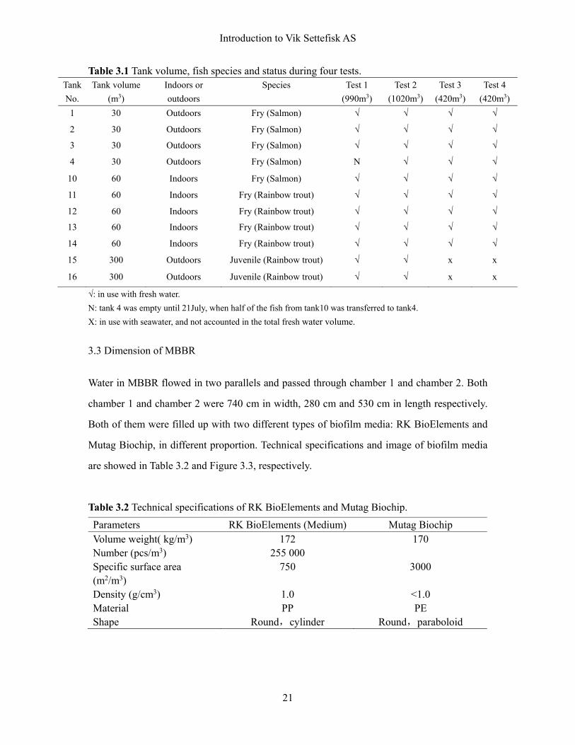
3.3 Dimension of MBBR

Water in MBBR flowed in two parallels and passed through chamber 1 and chamber 2. Both

chamber 1 and chamber 2 were 740 cm in width, 280 cm and 530 cm in length respectively.

Both of them were filled up with two different types of biofilm media: RK BioElements and

Mutag Biochip, in different proportion. Technical specifications and image of biofilm media

are showed in Table 3.2 and Figure 3.3, respectively.

Table 3.2 Technical specifications of RK BioElements and Mutag Biochip. Parameters RK BioElements (Medium) Mutag Biochip Volume weight( kg/m3) 172 170 Number (pcs/m3) 255 000 Specific surface area (m2/m3)

750 3000

Density (g/cm3) 1.0 <1.0 Material PP PE Shape Round，cylinder Round，paraboloid


22

Figure 3.3 Image of Mutag Biochip (left) and RK BioElements Medium.

In chamber 1, the depth of biofilm media is 65cm (when the chamber is drained of water), and

has the volume of 13.468 m3. While RK BioElements accounts for 75% in volume and the rest

26% is Mutag Biochip. Therefore, the total protected surface area in chamber 1 is 17 677 m2.

In chamber 2, the depth of biofilm media is 76cm (when the chamber is drained of water), and

has the volume of 29.807 m3. While RK BioElements accounts for 46% in volume and the rest

54% is Mutag Biochip. Therefore, the total protected surface area in chamber 1 is 58 571 m2.

The water level in the MBBR was maintained around 180cm. In operation, when biofilm

medias are immersed with water, the actual water volume is about 73.7%. Detailed information

about chamber 1 and chamber 2 are summarized in Table 3.3.

Table3.3 Detailed information about chamber1 and chamber 2. Chamber L*W*H (cm) Water

level(cm)Water volume(L)

Biomedia level(cm)

Biomedia volume(L)

% of media

Protected surface area m2

Chamber1 280*740*200 180 27487 65 13468 49.0 17 677 Chamber2 530*740*200 180 52029 76 29807 57.3 58 571


23

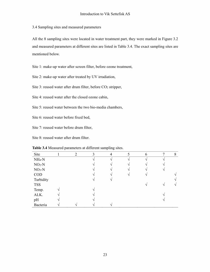
3.4 Sampling sites and measured parameters

All the 8 sampling sites were located in water treatment part, they were marked in Figure 3.2

and measured parameters at different sites are listed in Table 3.4. The exact sampling sites are

mentioned below. Site 1: make-up water after screen filter, before ozone treatment,

Site 2: make-up water after treated by UV irradiation,

Site 3: reused water after drum filter, before CO2 stripper,

Site 4: reused water after the closed ozone cabin,

Site 5: reused water between the two bio-media chambers,

Site 6: reused water before fixed bed,

Site 7: reused water before drum filter,

Site 8: reused water after drum filter.

Table 3.4 Measured parameters at different sampling sites.

Site 1 2 3 4 5 6 7 8NH4-N √ √ √ √ √ NO2-N √ √ √ √ √ NO3-N √ √ √ √ √ COD √ √ √ √ √Turbidity √ √ √TSS √ √ √Temp. √ √ ALK. √ √ √ pH √ √ √ Bacteria √ √ √ √

Materials and Methods

24

4. MATERIALS AND METHODS

This case study was carried out at the smolts farm of Vik Settefisk AS (Bergen). Detailed

information has been mentioned in Section 3, Introduction to Vik Settefisk AS. In total, four

tests has been conducted during the case study, and labelled as test 1, test 2, test 3 and test 4

respectively.

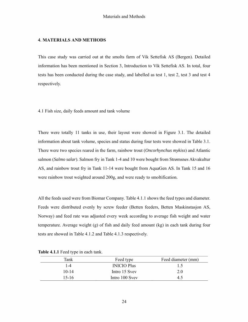
4.1 Fish size, daily feeds amount and tank volume

There were totally 11 tanks in use, their layout were showed in Figure 3.1. The detailed

information about tank volume, species and status during four tests were showed in Table 3.1.

There were two species reared in the farm, rainbow trout (Oncorhynchus mykiss) and Atlantic

salmon (Salmo salar). Salmon fry in Tank 1-4 and 10 were bought from Strømsnes Akvakultur

AS, and rainbow trout fry in Tank 11-14 were bought from AquaGen AS. In Tank 15 and 16

were rainbow trout weighted around 200g, and were ready to smoltification.

All the feeds used were from Biomar Company. Table 4.1.1 shows the feed types and diameter.

Feeds were distributed evenly by screw feeder (Betten feeders, Betten Maskinstasjon AS,

Norway) and feed rate was adjusted every week according to average fish weight and water

temperature. Average weight (g) of fish and daily feed amount (kg) in each tank during four

tests are showed in Table 4.1.2 and Table 4.1.3 respectively.

Table 4.1.1 Feed type in each tank. Tank Feed type Feed diameter (mm) 1-4 INICIO Plus 1.5

10-14 Intro 15 Svev 2.0 15-16 Intro 100 Svev 4.5


25

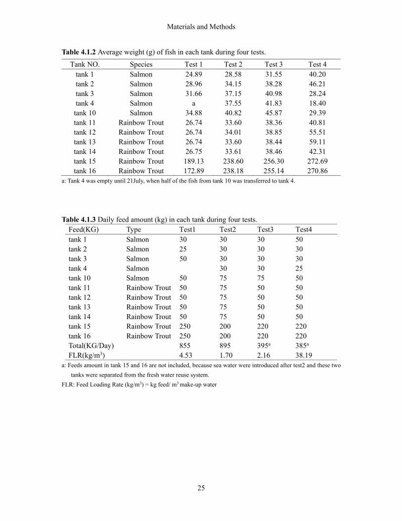
Table 4.1.2 Average weight (g) of fish in each tank during four tests.

Tank NO. Species Test 1 Test 2 Test 3 Test 4 tank 1 Salmon 24.89 28.58 31.55 40.20 tank 2 Salmon 28.96 34.15 38.28 46.21 tank 3 Salmon 31.66 37.15 40.98 28.24 tank 4 Salmon a 37.55 41.83 18.40 tank 10 Salmon 34.88 40.82 45.87 29.39 tank 11 Rainbow Trout 26.74 33.60 38.36 40.81 tank 12 Rainbow Trout 26.74 34.01 38.85 55.51 tank 13 Rainbow Trout 26.74 33.60 38.44 59.11 tank 14 Rainbow Trout 26.75 33.61 38.46 42.31 tank 15 Rainbow Trout 189.13 238.60 256.30 272.69 tank 16 Rainbow Trout 172.89 238.18 255.14 270.86

a: Tank 4 was empty until 21July, when half of the fish from tank 10 was transferred to tank 4.

Table 4.1.3 Daily feed amount (kg) in each tank during four tests. Feed(KG) Type Test1 Test2 Test3 Test4 tank 1 Salmon 30 30 30 50 tank 2 Salmon 25 30 30 30 tank 3 Salmon 50 30 30 30 tank 4 Salmon 30 30 25 tank 10 Salmon 50 75 75 50 tank 11 Rainbow Trout 50 75 50 50 tank 12 Rainbow Trout 50 75 50 50 tank 13 Rainbow Trout 50 75 50 50 tank 14 Rainbow Trout 50 75 50 50 tank 15 Rainbow Trout 250 200 220 220 tank 16 Rainbow Trout 250 200 220 220 Total(KG/Day) 855 895 395a 385a FLR(kg/m3) 4.53 1.70 2.16 38.19

a: Feeds amount in tank 15 and 16 are not included, because sea water were introduced after test2 and these two tanks were separated from the fresh water reuse system.

FLR: Feed Loading Rate (kg/m3) = kg feed/ m3 make-up water


26

4.2 Make-up water, recirculating rate and retention time

To compensate for the water loss and for water temperature adjustment purpose, make-up water

was taken from a nearby lake at depth of around 10 meters. The make-up water had stable

quality: temperature around 10 , pH ranged from 5.9 to 6.1 and a low alkalinity level around

5mg/L (as CaCO3).

After passing a screen filter, they were disinfected by both ozone gas (WEDECO, GSO 50) and

UV irradiation (WEDECO, B-80). Before entering the system, over-flow water was used to

increase temperature through a heat exchanger (Alfa Laval, TL6-BFM).

In test 1 and test 2, the fresh water flow rate was 7000 L/min; while in test 3 and test 4, seawater

had been introduced to tank 15 and tank 16, so the fresh water flow in the system was reduced

to 5000 L/min. Table 4.2 shows the make-up water flow, recirculating rate and retention during

the study.

Table 4.2 Make-up water flow, total fresh water flow, recirculating rate, and retention time in

chamber 1 and chamber 2 during four tests.

Test Make-up

water flow (L/min)

Total fresh water flow

(L/min)

Recirculating rate (%)

Retention time in chamber 1

(min)

Retention time in chamber 2

(min) 1 131 7000 98.13% 3.93 7.43

2 365 7000 94.79% 3.93 7.43

3 127 5000 97.46% 5.50 10.41

4 7 5000 99.86% 5.50 10.41


27

4. 3 UV and ozone dosage

UV (Wedeco GmbH, B-80, Herford, Germany) was used to disinfect make-up water. Table

4.3.1 shows technical information of the equipment.

Table 4.3.1 Technical information of UV instrument (WEDECO B-80). Parameters Characteristic Stainless steel reactor with multiple UV lamps Wave length, nm 254 B x H x T (mm) 1,295 x 430 x 270 UV Dose(w/m2) 300 (at the end of lamp lifetime) UV transmission 98% (at end of lamp lifetime) Application Drinking water; Process water; Warm water Capacity Up to 600 m3/h

During the experimental period, output of the UV light was 92.0 W/m2. The chamber for

irradiation is 51 L, and retention time differs depends on water flow. Table 4.3.2 shows UV

dosage in make-up water flow during four tests.

Table 4.3.2 UV dosage in make-up water flow.

Pure oxygen was used to generate ozone onsite (Wedeco GmbH, GSO 50, Herford, Germany).

The amount of ozone generated per hour (g/h) can be calculated according to the following

equation:

: The ozone quantity generated per hour (g/h),

A: power consumption on display (%),

: The maximum feed oxygen flow (5.7 m3/h for GSO 50 generator),

: Concentration of generated ozone (g/m3).

Test Output W/m2

Water flow(L/min)

Retention time(min)

UV dosage mJ/cm2

Test 1 92.0 78 0.65 358.8 Test 2 92.0 365 0.14 77.28 Test 3 92.0 127 0.40 220.8 Test 4 92.0 7 7.29 4024


28

In test 1 and 2, the ozone generator operated at 95% capacity (A=0.95). In test 3 and 4, the

generator operated at 60 % capacity (A=0.6). According to performance curve of the ozone

generator (Figure 4.3.1), in test 1 and 2 the concentration of generated ozone was 80 g/m3;

while in test 3 and 4, the concentration of generated ozone was 58 g/m3.

Ozone were distributed to disinfect both make-up water and reused water at different

percentage. Table 4.3.3 shows calculated ozone dosage in make-up and reused water.

Table 4.3.3 Ozone dosage in make-up water and reused water. Make-up water Reused water

Flow rate, L/min

Retention time, min

CO3， mg/L

Ozone C*t,Min*mg/L

Flow rate, L/min

Retention time, min

CO3, mg/L

Ozone C*t,Min*mg/L

Test 1 78 16.15 10 161.46 7000 3.43 0.97 3.34 Test 2 365 3.45 2.19 7.56 7000 3.43 0.97 3.34 Test 3 127 9.92 6.93 68.73 5000 4.8 0.93 4.44 Test 4 7 180 108 19542 5000 4.8 0.95 4.56

Figure 4.3 Performance curve (Vgas=5.70m3/h) of the ozone generator (Operation Instruction of EFFIZON Ozone Generator, GSO-50).


29

4. 4 Analysis of water quality

Water sample (500mL) was collected at depth of 50 cm at sampling sites (Figure 3.2), and

stored in polyethylene (PE) bottle for analysis. Parameters like dissolved oxygen, temperature

and pH were measured on site. Water sample was first used to measure heterotrophic bacteria

count and their turbidity, later the concentration of NH4-N, NO2-N, NO3-N and COD measured,

and in the end alkalinity and total suspended solids.

4.4.1Measurement of dissolved oxygen, temperature, pH

Dissolved oxygen, temperature were measured directly at sampling sites by a portable meter,

OxyGuard Handy Polaris 2 (OxyGuard International AS, Birkerød, Denmark). Dissolved

oxygen concentration are shown both in mg/L (or ppm) and in saturation (%), and temperature

is showed in degree Celsius (°C). pH was measured at each sampling site directly by portable

pH meter (OxyGuard Handy pH, Farum, Denmark).

4.4.2 Measurement of NH4-N, NO2-N, NO3-N and COD

Spectroquant® Photometer NOVA 60(Merck KGaA, Darmstadt, Germany) (Figure 4.4.1) was

used to determine the concentration of NH4-N, NO2- N, NO3- N and COD (mg/L). The first

three parameters were measured in a similar procedure (see Appendix 1-3), but using different

test kits.

In COD concentration measurement, thermoreactor (CR3200, Brannum Lane, Yellow Springs,

USA) was used. Pretreated water samples were incubated at 148 °C for 120 min in the

equipment. Detailed measurement procedures are listed in Appendix 4, and Table 4.4.1 shows

the characteristic quality data of the method.


30

Figure 4.4 Schematic diagram of Spectroquant® Photometer NOVA 60.

Table 4.4 Characteristic quality data of each parameter. Parameters NH4-N NO2- N NO3- N COD Cell(mm) 10 10 10 10 Standard deviation (mg/L) ±0.023 ±0.008 ±0.11 ±0.29 Co-efficiency of variation (%) ±1.5 ±1.4 ±0.85 ±1.4 Co-efficiency interval (mg/L) ±0.06 ±0.02 ±0.3 ±0.7 Number of lots 40 48 20 52 Measuring range (mg/L) 0.05-3.00 0.02-1.00 1.0-25 4.0-40.0 Accuracy of the measured value (mg/L) max.±0.08 max.±0.03 max.±0.5 max.±1.5Dilution times 4-8 4 4 2

4.4.3 Measurement of Alkalinity

Alkalinity was measured by titration 100mL water sample with hydrochloric acid (HCl, 0.1 M)

to the methyl orange endpoint (pH of 4.5). Then alkalinity is calculated by equation below:

Where: V1 is amount of hydrochloric acid used to reach pH 4.5 (mL)

C1 is the concentration of acid (mole/L)

V2 is the volume of water sample (mL)

Alkalinity is express in mg/L (as CaCO3).


31

4.4.4 Measurement of total suspended solids (TSS) and turbidity

TSS was measured by filtering well-mixed water sample through a weighted glass fiber filter

(0.45 µm, Whatman, GF/C), and then the filter was dried at 105°C. The weight increase of the

filter divided by the volume of water filtered is the concentration of total suspended solids; it

is expressed in mg/L. Turbidity was measured by nephelometer (Merck turbiquant 3000 IR), it

is expressed in NTU.

All analyzer instruments were calibrated before using.

4.4.5 Measurement of heterotrophic bacteria load

The heterotrophic bacteria load in terms of detection and enumeration was measured by a ready

to use, rehydrated plate with indicator (Compact Dry AQ, Uffing, Germany). At first 1 mL water sample was dropped in the middle of the plate, and then the water sample

was diffused into it and evenly spread on the plate, and then transformed the rehydrated plate

into a gel within seconds. After that put a cap on the plate and turned it over, then put it in an

incubator (at 36±2°C for 44±4h) in a horizontal position. After incubation, counted the number

of all grown colonies underneath the plate.

4.5 Statistical model

Results expressed in an average with standard deviation of three replicates. Statistical analysis

done by one-way ANOVA and statistical difference was considered to be significant if p < 0.05.


32

4.5.1 Calculation of TAN concentration from NH4-N concentration

As mentioned in literature review part, TAN is the sum of NH4-N and NH3-N, and the ratio

between NH4-N and NH3-N depends on temperature, salinity and pH. Based on NH4-N

concentration, TAN concentration can be calculated by equation below:

1

Where CTAN is TAN concentration (mg/L),

C NH4-N is measured NH4-N concentration (mg/L),

P NH3-N is the percent of NH3-N in TAN at different temperature and pH.

4.5.2 Calculation of areal TAN removal (ATR) rate

ATR is expressed in g/m2.d, which means g TAN removed per m2 surface area of bio-media

per day. Where Kc is the unit conversion constant (24h*60min/1000). TAN (a)-TAN (b) means

the TAN concentration difference (mg/L) between site a and site b. Q is the water flow rate in

the system (L/min). A is the protected surface area of bio-medias (m2).

4.5.3 Calculation of areal nitrite removal (ANR) rate

2. 2.

ANR is expressed in g/m2.d, which means g NO2-N removed per m2 surface area of bio-media

per day. Where Kc is the unit conversion constant (24h*60min/1000). NO2-N (a) - NO2-N (b)

means the NO2-N concentration difference (mg/L) between site a and site b. Q is the water flow

rate in the system (L/min). A is the protected surface area of bio-medias (m2).

Results

33

5. RESULTS

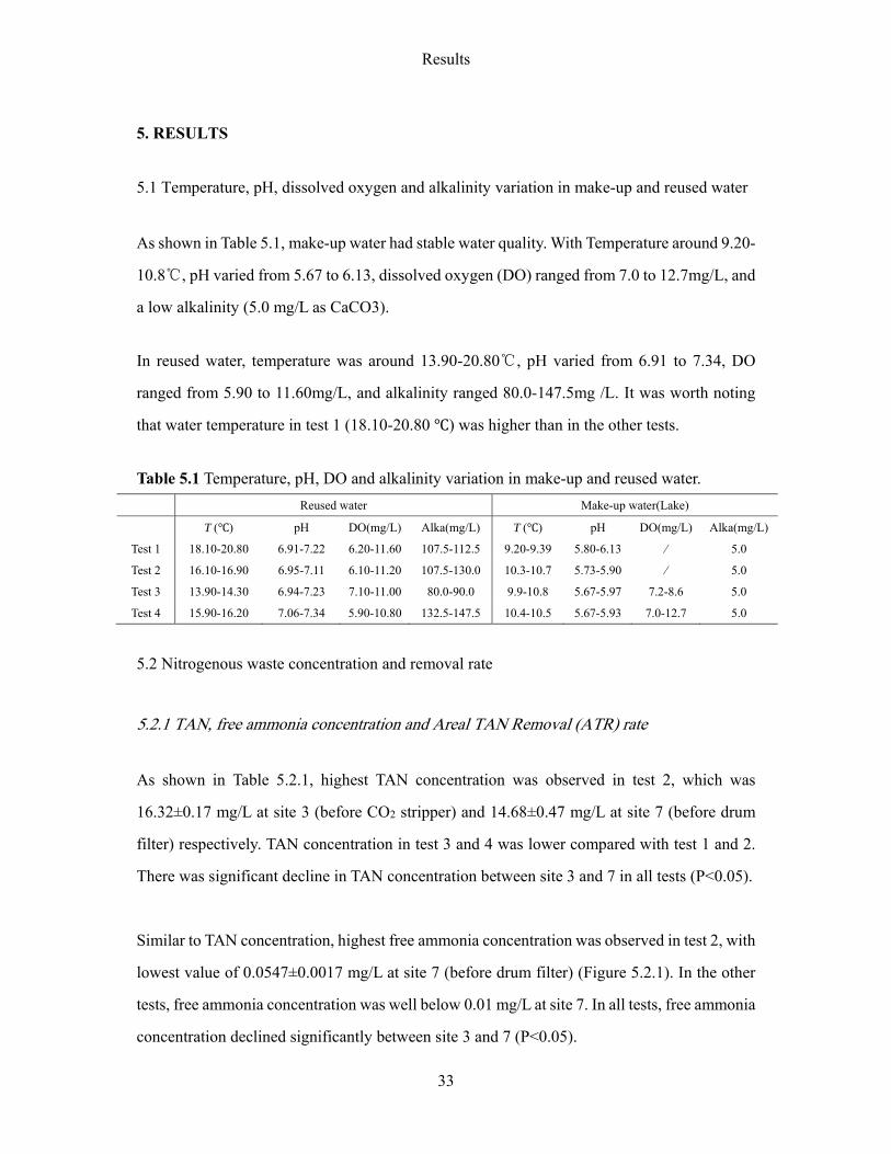
5.1 Temperature, pH, dissolved oxygen and alkalinity variation in make-up and reused water

As shown in Table 5.1, make-up water had stable water quality. With Temperature around 9.20-

10.8℃, pH varied from 5.67 to 6.13, dissolved oxygen (DO) ranged from 7.0 to 12.7mg/L, and

a low alkalinity (5.0 mg/L as CaCO3). In reused water, temperature was around 13.90-20.80℃, pH varied from 6.91 to 7.34, DO

ranged from 5.90 to 11.60mg/L, and alkalinity ranged 80.0-147.5mg /L. It was worth noting

that water temperature in test 1 (18.10-20.80 ) was higher than in the other tests. Table 5.1 Temperature, pH, DO and alkalinity variation in make-up and reused water.

Reused water Make-up water(Lake)

T ( ) pH DO(mg/L) Alka(mg/L) T ( ) pH DO(mg/L) Alka(mg/L)

Test 1 18.10-20.80 6.91-7.22 6.20-11.60 107.5-112.5 9.20-9.39 5.80-6.13 ⁄ 5.0

Test 2 16.10-16.90 6.95-7.11 6.10-11.20 107.5-130.0 10.3-10.7 5.73-5.90 ⁄ 5.0

Test 3 13.90-14.30 6.94-7.23 7.10-11.00 80.0-90.0 9.9-10.8 5.67-5.97 7.2-8.6 5.0

Test 4 15.90-16.20 7.06-7.34 5.90-10.80 132.5-147.5 10.4-10.5 5.67-5.93 7.0-12.7 5.0

5.2 Nitrogenous waste concentration and removal rate

5.2.1 TAN, free ammonia concentration and Areal TAN Removal (ATR) rate

As shown in Table 5.2.1, highest TAN concentration was observed in test 2, which was

16.32±0.17 mg/L at site 3 (before CO2 stripper) and 14.68±0.47 mg/L at site 7 (before drum

filter) respectively. TAN concentration in test 3 and 4 was lower compared with test 1 and 2.

There was significant decline in TAN concentration between site 3 and 7 in all tests (P<0.05).

Similar to TAN concentration, highest free ammonia concentration was observed in test 2, with

lowest value of 0.0547±0.0017 mg/L at site 7 (before drum filter) (Figure 5.2.1). In the other

tests, free ammonia concentration was well below 0.01 mg/L at site 7. In all tests, free ammonia

concentration declined significantly between site 3 and 7 (P<0.05).

Results

34

Table 5.2.1 TAN concentration (mg/L) at different sites during four tests (M±SD. Site 3: before CO2 stripper; site 4: after ozone cabin; site 5: between MBBR; site 6: after MBBR; site 7: before drum filter). n=3 Site 3 Site 4 Site 5 Site 6 Site 7

Test 1 3.63±0.05 2.99±0.09 2.68±0.08 1.57±0.00 1.27±0.08 Test 2 16.32±0.17 15.88±0.08 15.11±0.62 14.68±0.26 14.68±0.47 Test 3 1.44±0.23 1.45±0.06 1.10±0.05 0.49±0.02 0.49±0.02 Test 4 2.31±0.02 1.88±0.05 1.30±0.11 0.52±0.03 0.58±0.12

Figure 5.2.1 Free ammonia concentration (mg/L) variation at different sites during four tests (M ±SD. Site 3: before CO2 stripper; site 4: after ozone cabin; site 5: between MBBR; site 6: after MBBR; site 7: before drum filter, n=3).

Table 5.2.2 Areal TAN removal rate (g/m2.d) in MBBR during four tests (M ±SD. Chamber 1: site 4-5, Chamber 2: site 5-6. Site 4: after ozone cabin; site 5: between MBBR; site 6: after MBBR).

n=3 Chamber 1 Chamber 2 Total, MBBR Test 1 0.176 ± 0.022 0.193 ± 0.014 0.369 ± 0.027 Test 2 0.439 ± 0.329 0.074 ± 0.143 0.513 ± 0.186 Test 3 0.142 ± 0.034 0.074 ± 0.007 0.216 ± 0.027 Test 4 0.235 ± 0.062 0.096 ± 0.013 0.330 ± 0.049

Together with highest free ammonia and TAN concentration, the highest areal TAN removal

(ATR) rate was also observed in test 2 (Table 5.2.2), which was 0.513±0.186 g/m2.d. In test 1,

chamber 1 and 2 had similar efficiency. While in test 3 and 4, chamber 1 showed higher

efficiency than chamber 2. As shown in Figure 5.2.2, increased average TAN concentration

resulted in a higher ATR rate.

0.0000

0.0200

0.0400

0.0600

0.0800

0.1000

Site3 Site4 Site5 Site6 Site7

Free

ammonia , mg/L

Test1 Test2 Test3 Test4

Results

35

Figure 5.2.2 Areal TAN removal rate (g/m2.d) in chamber1 and chamber2 during four tests (Chamber 1: site 4-5, Chamber 2: site 5-6. Site 4: after ozone cabin; site 5: between MBBR; site 6: after MBBR).

As shown in Table 5.2.3, constant reduction in TAN concentration was only observed in test 1.

In test 2, TAN reduction percent was low due to high initial TAN concentration (16.32±0.17

mg/L at site 3). It is worth noting that except in test 3, TAN concentration showed reduction

between site 3 and 4 (water passed through CO2 stripper and closed ozone cabin). In addition,

chamber 2 (S5-S6) had higher TAN reduction percent than chamber 1 (S4-S5), except in test 2

when TAN reduction percent were low in both chambers.

Table 5.2.3 TAN reduction percent (%) between each site（M ±SD. Site 3:before CO2 stripper; site 4:after ozone cabin; site 5: between MBBR; site 6: after MBBR; site 7: before drum filter）. n=3 S3-S4 S4-S5 S5-S6 S6-S7 Test 1 17.52±1.93 10.30±1.12 41.62±1.81 18.80±4.83 Test 2 2.68±1.50 4.86±3.63 2.62±5.46 -0.01±2.98 Test 3 -1.94±11.27 23.93±4.98 54.84±2.84 -0.21±6.54 Test 4 18.91±2.71 30.53±7.45 59.58±3.71 -9.62±15.15

2.428

15.334

0.9941.318

0

2

4

6

8

10

12

14

16

18

0.000

0.100

0.200

0.300

0.400

0.500

0.600

0.700

0.800

0.900

1.000


TAN concentration, m

g/L

ATR

, g/m

2.d

Chamber1, ATR

Chamber2, ATR

Total (C1+C2), ATR

Average TANconcentration, mg/L

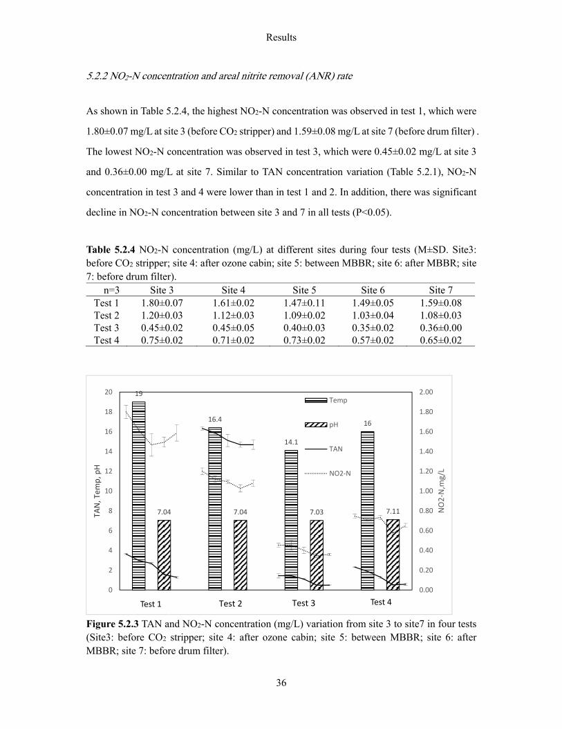
Results

36

5.2.2 NO2-N concentration and areal nitrite removal (ANR) rate

As shown in Table 5.2.4, the highest NO2-N concentration was observed in test 1, which were

1.80±0.07 mg/L at site 3 (before CO2 stripper) and 1.59±0.08 mg/L at site 7 (before drum filter) .

The lowest NO2-N concentration was observed in test 3, which were 0.45±0.02 mg/L at site 3

and 0.36±0.00 mg/L at site 7. Similar to TAN concentration variation (Table 5.2.1), NO2-N

concentration in test 3 and 4 were lower than in test 1 and 2. In addition, there was significant

decline in NO2-N concentration between site 3 and 7 in all tests (P<0.05).

Table 5.2.4 NO2-N concentration (mg/L) at different sites during four tests (M±SD. Site3: before CO2 stripper; site 4: after ozone cabin; site 5: between MBBR; site 6: after MBBR; site 7: before drum filter). n=3 Site 3 Site 4 Site 5 Site 6 Site 7 Test 1 1.80±0.07 1.61±0.02 1.47±0.11 1.49±0.05 1.59±0.08 Test 2 1.20±0.03 1.12±0.03 1.09±0.02 1.03±0.04 1.08±0.03 Test 3 0.45±0.02 0.45±0.05 0.40±0.03 0.35±0.02 0.36±0.00 Test 4 0.75±0.02 0.71±0.02 0.73±0.02 0.57±0.02 0.65±0.02

Figure 5.2.3 TAN and NO2-N concentration (mg/L) variation from site 3 to site7 in four tests (Site3: before CO2 stripper; site 4: after ozone cabin; site 5: between MBBR; site 6: after MBBR; site 7: before drum filter).

19

16.4

14.1

16

7.04 7.04 7.03 7.11

0.00

0.20

0.40

0.60

0.80

1.00

1.20

1.40

1.60

1.80

2.00

0

2

4

6

8

10

12

14

16

18

20

NO2‐N,m

g/L

TAN, Tem

p, pH

Temp

pH

TAN

NO2‐N

Test 2 Test 3Test 1 Test 4

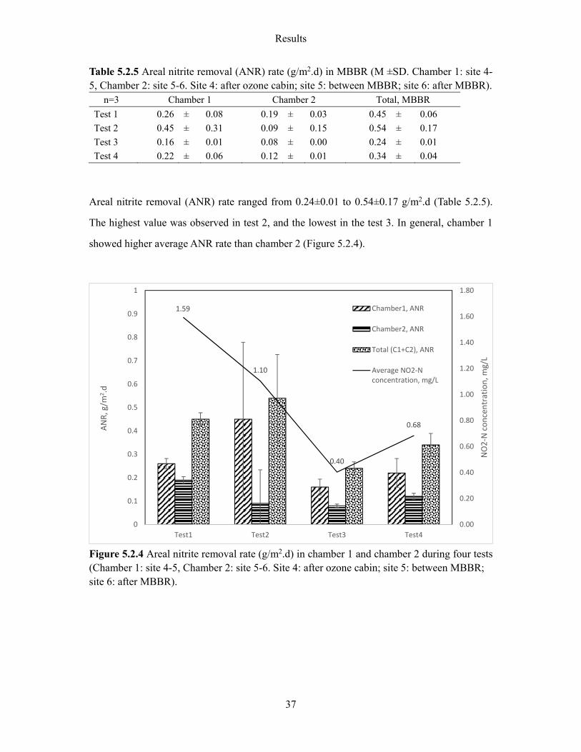
Results

37

Table 5.2.5 Areal nitrite removal (ANR) rate (g/m2.d) in MBBR (M ±SD. Chamber 1: site 4-5, Chamber 2: site 5-6. Site 4: after ozone cabin; site 5: between MBBR; site 6: after MBBR). n=3 Chamber 1 Chamber 2 Total, MBBR Test 1 0.26 ± 0.08 0.19 ± 0.03 0.45 ± 0.06 Test 2 0.45 ± 0.31 0.09 ± 0.15 0.54 ± 0.17 Test 3 0.16 ± 0.01 0.08 ± 0.00 0.24 ± 0.01 Test 4 0.22 ± 0.06 0.12 ± 0.01 0.34 ± 0.04

Areal nitrite removal (ANR) rate ranged from 0.24±0.01 to 0.54±0.17 g/m2.d (Table 5.2.5).

The highest value was observed in test 2, and the lowest in the test 3. In general, chamber 1

showed higher average ANR rate than chamber 2 (Figure 5.2.4).

Figure 5.2.4 Areal nitrite removal rate (g/m2.d) in chamber 1 and chamber 2 during four tests (Chamber 1: site 4-5, Chamber 2: site 5-6. Site 4: after ozone cabin; site 5: between MBBR; site 6: after MBBR).

1.59

1.10

0.40

0.68

0.00

0.20

0.40

0.60

0.80

1.00

1.20

1.40

1.60

1.80

0

0.1

0.2

0.3

0.4

0.5

0.6

0.7

0.8

0.9

1


NO2‐N concentration, m

g/L

ANR, g/m

2 .d

Chamber1, ANR

Chamber2, ANR

Total (C1+C2), ANR

Average NO2‐Nconcentration, mg/L

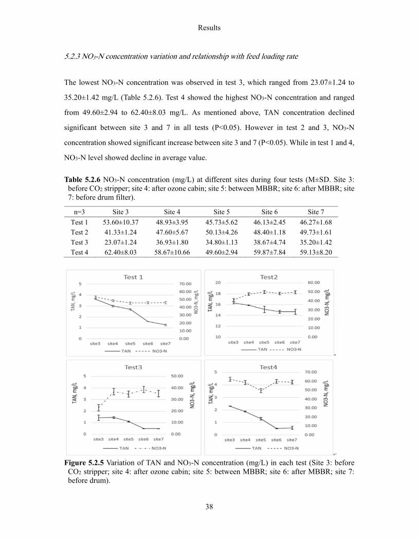
Results

38

5.2.3 NO3-N concentration variation and relationship with feed loading rate

The lowest NO3-N concentration was observed in test 3, which ranged from 23.07±1.24 to

35.20±1.42 mg/L (Table 5.2.6). Test 4 showed the highest NO3-N concentration and ranged

from 49.60±2.94 to 62.40±8.03 mg/L. As mentioned above, TAN concentration declined

significant between site 3 and 7 in all tests (P<0.05). However in test 2 and 3, NO3-N

concentration showed significant increase between site 3 and 7 (P<0.05). While in test 1 and 4,

NO3-N level showed decline in average value. Table 5.2.6 NO3-N concentration (mg/L) at different sites during four tests (M±SD. Site 3:

before CO2 stripper; site 4: after ozone cabin; site 5: between MBBR; site 6: after MBBR; site 7: before drum filter).

Figure 5.2.5 Variation of TAN and NO3-N concentration (mg/L) in each test (Site 3: before

CO2 stripper; site 4: after ozone cabin; site 5: between MBBR; site 6: after MBBR; site 7: before drum).

n=3 Site 3 Site 4 Site 5 Site 6 Site 7 Test 1 53.60±10.37 48.93±3.95 45.73±5.62 46.13±2.45 46.27±1.68 Test 2 41.33±1.24 47.60±5.67 50.13±4.26 48.40±1.18 49.73±1.61 Test 3 23.07±1.24 36.93±1.80 34.80±1.13 38.67±4.74 35.20±1.42 Test 4 62.40±8.03 58.67±10.66 49.60±2.94 59.87±7.84 59.13±8.20

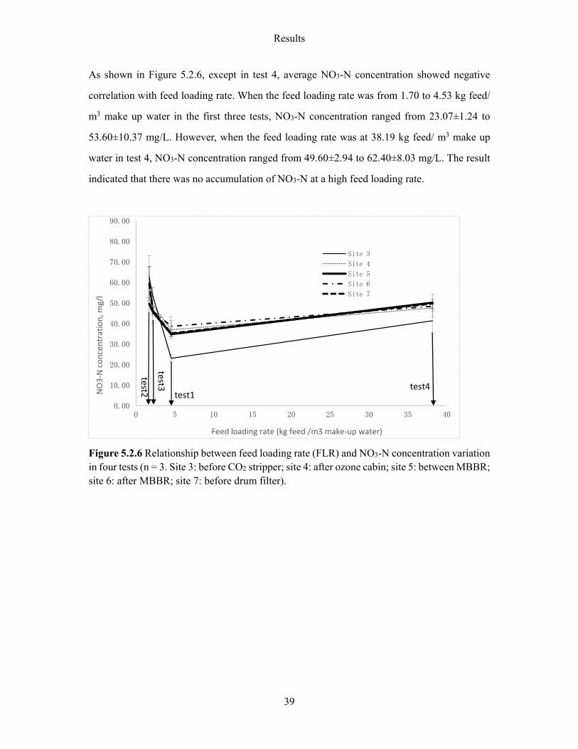
Results

39

As shown in Figure 5.2.6, except in test 4, average NO3-N concentration showed negative

correlation with feed loading rate. When the feed loading rate was from 1.70 to 4.53 kg feed/

m3 make up water in the first three tests, NO3-N concentration ranged from 23.07±1.24 to

53.60±10.37 mg/L. However, when the feed loading rate was at 38.19 kg feed/ m3 make up

water in test 4, NO3-N concentration ranged from 49.60±2.94 to 62.40±8.03 mg/L. The result

indicated that there was no accumulation of NO3-N at a high feed loading rate.

Figure 5.2.6 Relationship between feed loading rate (FLR) and NO3-N concentration variation in four tests (n = 3. Site 3: before CO2 stripper; site 4: after ozone cabin; site 5: between MBBR; site 6: after MBBR; site 7: before drum filter).

0.00

10.00

20.00

30.00

40.00

50.00

60.00

70.00

80.00

90.00

0 5 10 15 20 25 30 35 40

NO3‐N concentration, m

g/l

Feed loading rate (kg feed /m3 make‐up water)

Site 3

Site 4

Site 5

Site 6

Site 7

test4test1

test2

test3

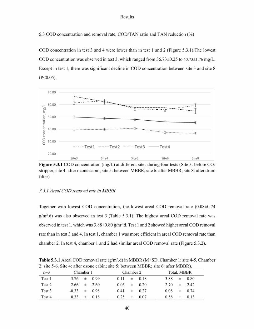
Results

40

5.3 COD concentration and removal rate, COD/TAN ratio and TAN reduction (%)

COD concentration in test 3 and 4 were lower than in test 1 and 2 (Figure 5.3.1).The lowest

COD concentration was observed in test 3, which ranged from 36.73±0.25 to 40.73±1.76 mg/L.

Except in test 1, there was significant decline in COD concentration between site 3 and site 8

(P<0.05).

Figure 5.3.1 COD concentration (mg/L) at different sites during four tests (Site 3: before CO2 stripper; site 4: after ozone cabin; site 5: between MBBR; site 6: after MBBR; site 8: after drum filter)

5.3.1 Areal COD removal rate in MBBR

Together with lowest COD concentration, the lowest areal COD removal rate (0.08±0.74

g/m2.d) was also observed in test 3 (Table 5.3.1). The highest areal COD removal rate was

observed in test 1, which was 3.88±0.80 g/m2.d. Test 1 and 2 showed higher areal COD removal

rate than in test 3 and 4. In test 1, chamber 1 was more efficient in areal COD removal rate than

chamber 2. In test 4, chamber 1 and 2 had similar areal COD removal rate (Figure 5.3.2).

Table 5.3.1 Areal COD removal rate (g/m2.d) in MBBR (M±SD. Chamber 1: site 4-5, Chamber 2: site 5-6. Site 4: after ozone cabin; site 5: between MBBR; site 6: after MBBR).

n=3 Chamber 1 Chamber 2 Total, MBBR Test 1 3.76 ± 0.99 0.11 ± 0.18 3.88 ± 0.80 Test 2 2.66 ± 2.60 0.03 ± 0.20 2.70 ± 2.42 Test 3 -0.33 ± 0.98 0.41 ± 0.27 0.08 ± 0.74 Test 4 0.33 ± 0.18 0.25 ± 0.07 0.58 ± 0.13

20.00

30.00

40.00

50.00

60.00

70.00

Site3 Site4 Site5 Site6 Site8

COD concentration, m

g/L


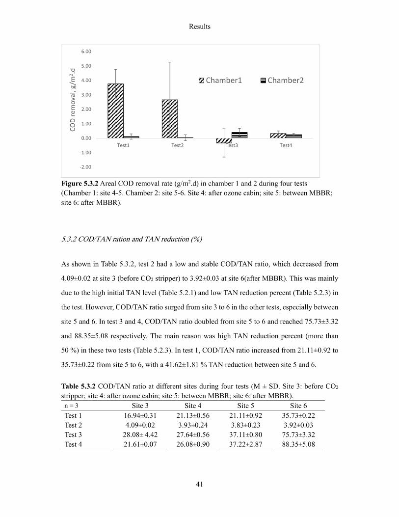
Results

41

Figure 5.3.2 Areal COD removal rate (g/m2.d) in chamber 1 and 2 during four tests (Chamber 1: site 4-5. Chamber 2: site 5-6. Site 4: after ozone cabin; site 5: between MBBR; site 6: after MBBR).

5.3.2 COD/TAN ration and TAN reduction (%)

As shown in Table 5.3.2, test 2 had a low and stable COD/TAN ratio, which decreased from

4.09±0.02 at site 3 (before CO2 stripper) to 3.92±0.03 at site 6(after MBBR). This was mainly

due to the high initial TAN level (Table 5.2.1) and low TAN reduction percent (Table 5.2.3) in

the test. However, COD/TAN ratio surged from site 3 to 6 in the other tests, especially between

site 5 and 6. In test 3 and 4, COD/TAN ratio doubled from site 5 to 6 and reached 75.73±3.32

and 88.35±5.08 respectively. The main reason was high TAN reduction percent (more than

50 %) in these two tests (Table 5.2.3). In test 1, COD/TAN ratio increased from 21.11±0.92 to

35.73±0.22 from site 5 to 6, with a 41.62±1.81 % TAN reduction between site 5 and 6. Table 5.3.2 COD/TAN ratio at different sites during four tests (M ± SD. Site 3: before CO2 stripper; site 4: after ozone cabin; site 5: between MBBR; site 6: after MBBR). n = 3 Site 3 Site 4 Site 5 Site 6 Test 1 16.94±0.31 21.13±0.56 21.11±0.92 35.73±0.22 Test 2 4.09±0.02 3.93±0.24 3.83±0.23 3.92±0.03 Test 3 28.08± 4.42 27.64±0.56 37.11±0.80 75.73±3.32 Test 4 21.61±0.07 26.08±0.90 37.22±2.87 88.35±5.08

‐2.00

‐1.00

0.00

1.00

2.00

3.00

4.00

5.00

6.00


COD removal, g/m

2.d

Chamber1 Chamber2

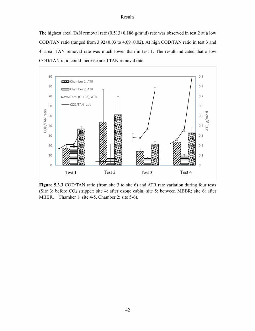
Results

42

The highest areal TAN removal rate (0.513±0.186 g/m2.d) rate was observed in test 2 at a low

COD/TAN ratio (ranged from 3.92±0.03 to 4.09±0.02). At high COD/TAN ratio in test 3 and

4, areal TAN removal rate was much lower than in test 1. The result indicated that a low

COD/TAN ratio could increase areal TAN removal rate.

Figure 5.3.3 COD/TAN ratio (from site 3 to site 6) and ATR rate variation during four tests (Site 3: before CO2 stripper; site 4: after ozone cabin; site 5: between MBBR; site 6: after MBBR. Chamber 1: site 4-5. Chamber 2: site 5-6).

0

0.1

0.2

0.3

0.4

0.5

0.6

0.7

0.8

0.9

0

10

20

30

40

50

60

70

80

90

ATR

, g/m

2.d

COD/TAN ratio

Chamber 1, ATR

Chamber 2, ATR

Total (C1+C2), ATR

COD/TAN ratio

Test 2 Test 3 Test 4Test 1

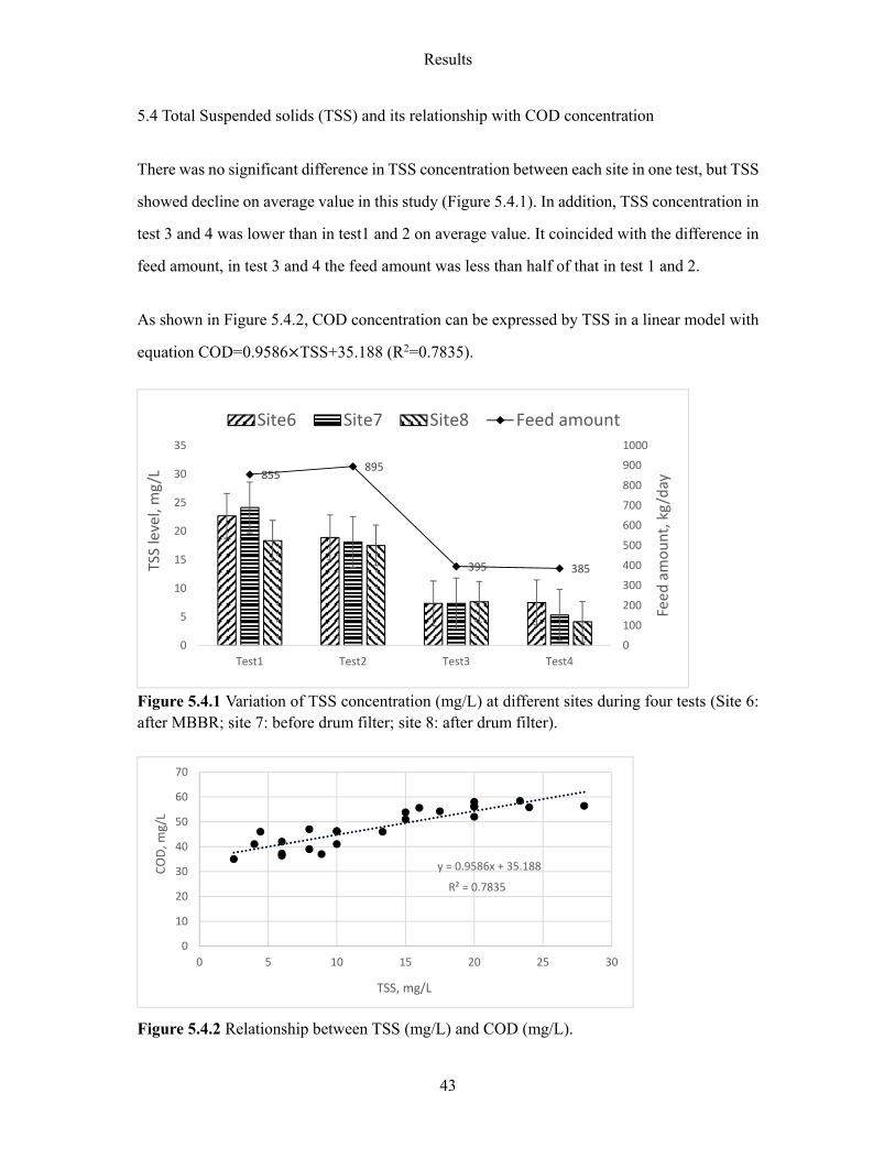
Results

43

5.4 Total Suspended solids (TSS) and its relationship with COD concentration

There was no significant difference in TSS concentration between each site in one test, but TSS

showed decline on average value in this study (Figure 5.4.1). In addition, TSS concentration in

test 3 and 4 was lower than in test1 and 2 on average value. It coincided with the difference in

feed amount, in test 3 and 4 the feed amount was less than half of that in test 1 and 2. As shown in Figure 5.4.2, COD concentration can be expressed by TSS in a linear model with

equation COD=0.9586 TSS+35.188 (R2=0.7835).

Figure 5.4.1 Variation of TSS concentration (mg/L) at different sites during four tests (Site 6: after MBBR; site 7: before drum filter; site 8: after drum filter).

Figure 5.4.2 Relationship between TSS (mg/L) and COD (mg/L).

855895

395 385

0

100

200

300

400

500

600

700

800

900

1000

0

5

10

15

20

25

30

35

Test1 Test2 Test3 Test4Feed

amount, kg/day

TSS level, mg/L

Site6 Site7 Site8 Feed amount

R² = 0.7835

y = 0.9586x + 35.188

0

10

20

30

40

50

60

70

0 5 10 15 20 25 30

COD, m

g/L

TSS, mg/L

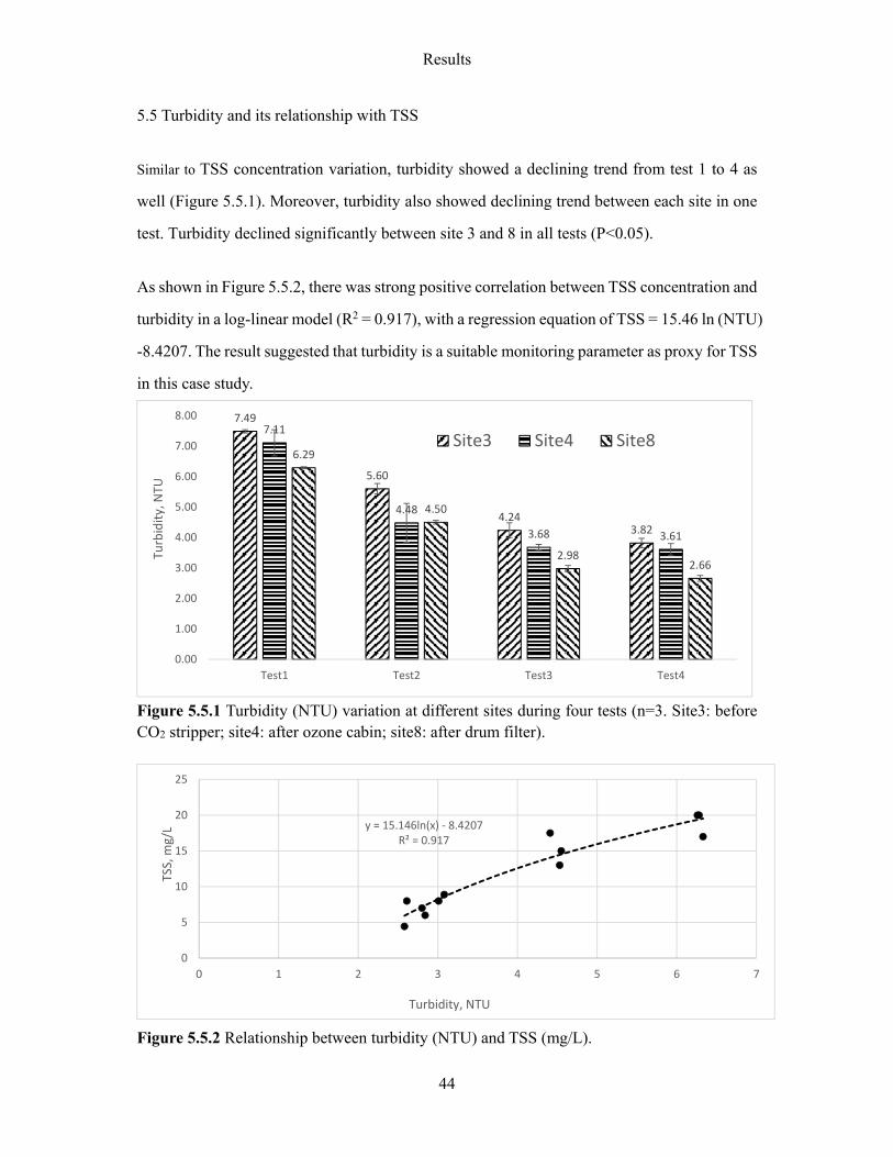
Results

44

5.5 Turbidity and its relationship with TSS

Similar to TSS concentration variation, turbidity showed a declining trend from test 1 to 4 as

well (Figure 5.5.1). Moreover, turbidity also showed declining trend between each site in one

test. Turbidity declined significantly between site 3 and 8 in all tests (P<0.05).

As shown in Figure 5.5.2, there was strong positive correlation between TSS concentration and

turbidity in a log-linear model (R2 = 0.917), with a regression equation of TSS = 15.46 ln (NTU)

-8.4207. The result suggested that turbidity is a suitable monitoring parameter as proxy for TSS

in this case study.

Figure 5.5.1 Turbidity (NTU) variation at different sites during four tests (n=3. Site3: before CO2 stripper; site4: after ozone cabin; site8: after drum filter).

Figure 5.5.2 Relationship between turbidity (NTU) and TSS (mg/L).

7.49

5.60

4.243.82

7.11

4.48

3.68 3.61

6.29

4.50

2.982.66

0.00

1.00

2.00

3.00

4.00

5.00

6.00

7.00

8.00


Turbidity, NTU

Site3 Site4 Site8

y = 15.146ln(x) ‐ 8.4207R² = 0.917

0

5

10

15

20

25

0 1 2 3 4 5 6 7

TSS, m

g/L

Turbidity, NTU

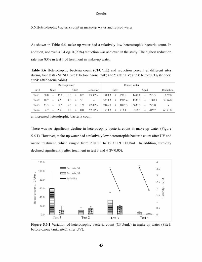
Results

45

5.6 Heterotrophic bacteria count in make-up water and reused water

As shown in Table 5.6, make-up water had a relatively low heterotrophic bacteria count. In

addition, not even a 1-Log10 (90%) reduction was achieved in the study. The highest reduction

rate was 83% in test 1 of treatment in make-up water. Table 5.6 Heterotrophic bacteria count (CFU/mL) and reduction percent at different sites during four tests (M±SD. Site1: before ozone tank; site2: after UV; site3: before CO2 stripper; site4: after ozone cabin).

Make-up water Reused water

n=3 Site1 Site2 Reduction Site3 Site4 Reduction

Test1 60.0 ± 35.6 10.0 ± 8.2 83.33% 1703.3 ± 295.8 1490.0 ± 283.3 12.52%

Test2 10.7 ± 5.2 14.0 ± 5.1 a 3233.3 ± 1975.4 1333.3 ± 1007.7 58.76%

Test3 33.3 ± 17.5 19.3 ± 1.9 42.00% 2166.7 ± 1087.3 3633.3 ± 793.0 a

Test4 4.7 ± 2.5 2.0 ± 0.0 57.14% 933.3 ± 713.4 366.7 ± 449.7 60.71%

a: increased heterotrophic bacteria count There was no significant decline in heterotrophic bacteria count in make-up water (Figure

5.6.1). However, make-up water had a relatively low heterotrophic bacteria count after UV and

ozone treatment, which ranged from 2.0±0.0 to 19.3±1.9 CFU/mL. In addition, turbidity

declined significantly after treatment in test 3 and 4 (P<0.05).

Figure 5.6.1 Variation of heterotrophic bacteria count (CFU/mL) in make-up water (Site1: before ozone tank; site2: after UV).

0

0.5

1

1.5

2

2.5

3

3.5

4

0.0

20.0

40.0

60.0

80.0

100.0

120.0Turbidity，

NTU

Bacteria count，

CFU

/mL

Bacteria, S1

Bacteria, S2

Turbidity

Test 2 Test 4Test 3Test 1

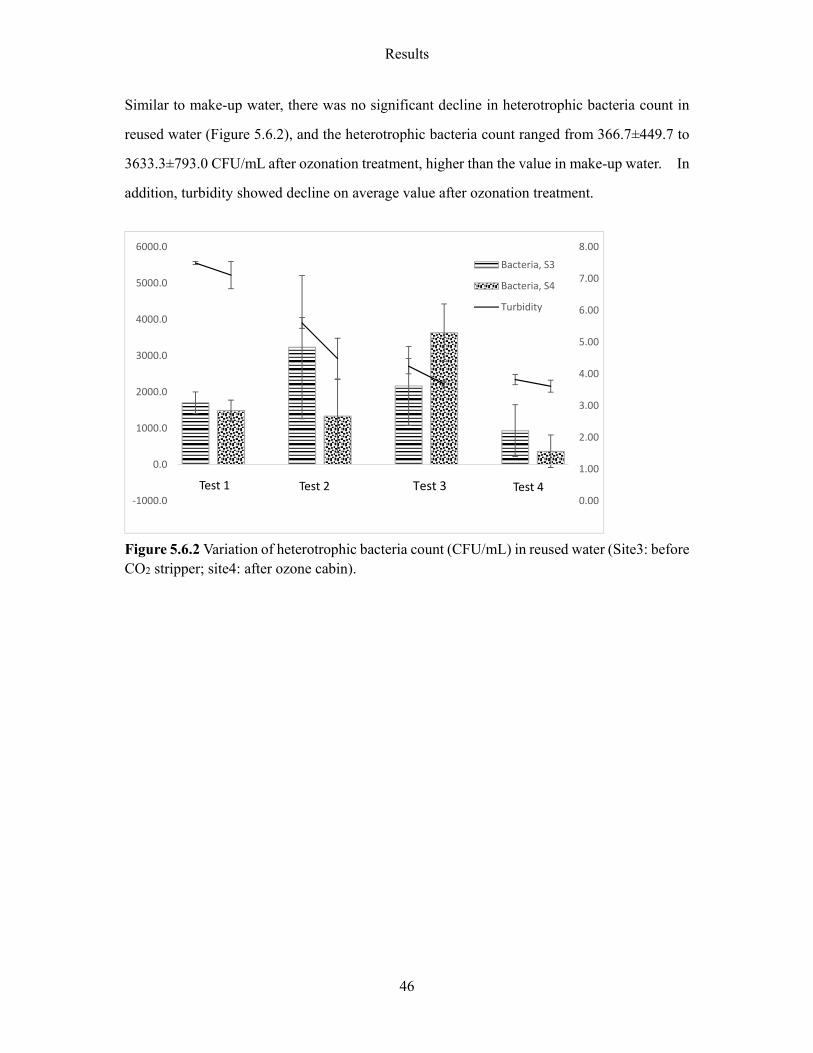
Results

46

Similar to make-up water, there was no significant decline in heterotrophic bacteria count in

reused water (Figure 5.6.2), and the heterotrophic bacteria count ranged from 366.7±449.7 to

3633.3±793.0 CFU/mL after ozonation treatment, higher than the value in make-up water. In

addition, turbidity showed decline on average value after ozonation treatment.

Figure 5.6.2 Variation of heterotrophic bacteria count (CFU/mL) in reused water (Site3: before CO2 stripper; site4: after ozone cabin).

0.00

1.00

2.00

3.00

4.00

5.00

6.00

7.00

8.00

‐1000.0

0.0

1000.0

2000.0

3000.0

4000.0

5000.0

6000.0

Bacteria, S3

Bacteria, S4

Turbidity

Test 3Test 1 Test 2 Test 4

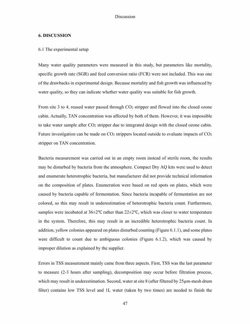
Discussion

47

6. DISCUSSION

6.1 The experimental setup

Many water quality parameters were measured in this study, but parameters like mortality,

specific growth rate (SGR) and feed conversion ratio (FCR) were not included. This was one

of the drawbacks in experimental design. Because mortality and fish growth was influenced by

water quality, so they can indicate whether water quality was suitable for fish growth. From site 3 to 4, reused water passed through CO2 stripper and flowed into the closed ozone

cabin. Actually, TAN concentration was affected by both of them. However, it was impossible

to take water sample after CO2 stripper due to integrated design with the closed ozone cabin.

Future investigation can be made on CO2 strippers located outside to evaluate impacts of CO2

stripper on TAN concentration. Bacteria measurement was carried out in an empty room instead of sterile room, the results

may be disturbed by bacteria from the atmosphere. Compact Dry AQ kits were used to detect

and enumerate heterotrophic bacteria, but manufacturer did not provide technical information

on the composition of plates. Enumeration were based on red spots on plates, which were

caused by bacteria capable of fermentation. Since bacteria incapable of fermentation are not

colored, so this may result in underestimation of heterotrophic bacteria count. Furthermore,

samples were incubated at 36±2 rather than 22±2 , which was closer to water temperature

in the system. Therefore, this may result in an incredible heterotrophic bacteria count. In

addition, yellow colonies appeared on plates disturbed counting (Figure 6.1.1), and some plates

were difficult to count due to ambiguous colonies (Figure 6.1.2), which was caused by

improper dilution as explained by the supplier. Errors in TSS measurement mainly came from three aspects. First, TSS was the last parameter

to measure (2-3 hours after sampling), decomposition may occur before filtration process,

which may result in underestimation. Second, water at site 8 (after filtered by 25µm-mesh drum

filter) contains low TSS level and 1L water (taken by two times) are needed to finish the

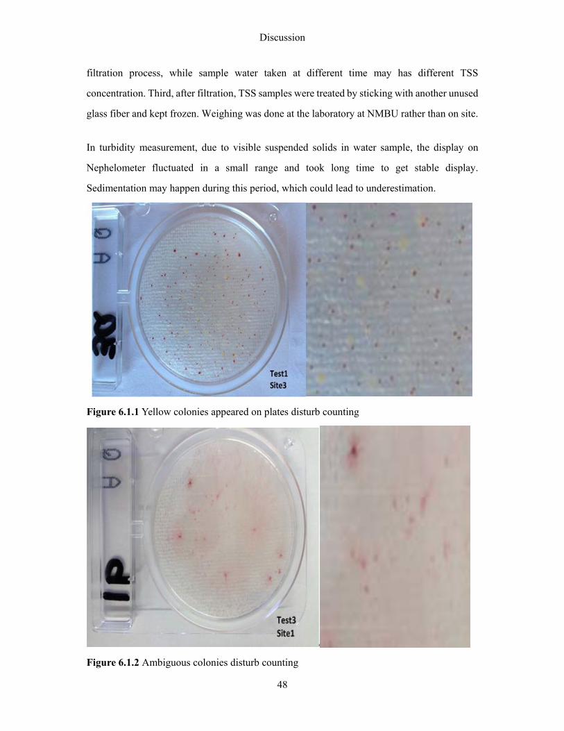
Discussion

48

filtration process, while sample water taken at different time may has different TSS

concentration. Third, after filtration, TSS samples were treated by sticking with another unused

glass fiber and kept frozen. Weighing was done at the laboratory at NMBU rather than on site. In turbidity measurement, due to visible suspended solids in water sample, the display on

Nephelometer fluctuated in a small range and took long time to get stable display.

Sedimentation may happen during this period, which could lead to underestimation.

Figure 6.1.1 Yellow colonies appeared on plates disturb counting

Figure 6.1.2 Ambiguous colonies disturb counting

Discussion

49

6.2 Discussion of water quality and MBBR performance

6.2.1 TAN, NO2-N concentration and removal rate

Due to its high toxicity to fish, free ammonia accumulation is one of the most notorious

problems in RAS (Hargreaves, 1998). Molleda et al. (2007) study in a RAS for arctic charr

(Salvelinus alpinus) farm found that free ammonia concentration ranges from 0.001-0.014

mg/L in outlet water from fish tanks and 0.002-0.018 mg/L in outlet water from the bio filter

unit. In this study, higher values were observed. Especially in test 2, free ammonia

concentration at all sites were above 0.05 mg/L, which was two times higher than the

recommended maximum concentration (0.025mg/L) in intensive fish farming (Chen et al.,

2006). While in the other tests, free ammonia concentration at site 7 were only around 0.005

mg/L, well below the recommended value.

In the same study from Molleda et al. (2007), TAN concentration was around 0.251-1.520 mg/L

in outlet from fish tanks and 0.246-1.577 mg/L in outlet from the bio filter unit. Higher values

were observed in this study also. In test 2, TAN level was above 15 mg/L at all sites, which

was higher than the recommended concentration (1.0 mg/L) for long-term exposure (Losordo

et al., 1998). TAN levels observed in test1 were also higher than in test 3 (0.49±0.02 to

1.44±0.23 mg/L) and test 4 (0.58±0.12 to 2.31±0.02 mg/L).

This difference can be explained by variations in feeding amount. 855 kg/day and 895 kg/day

feed were used in test 1 and 2, while in test 3 and 4, it was only 395 kg/day and 385 kg/day. In

addition, one day before test 2, there were uneaten feed floating in tank 15 and tank 16, and the

film of first drum filter was partially blocked by uneaten feed.

In another study at a running warm water RAS for Nile tilapia, Ding (2012) found areal TAN

removal rate range from 0.14-0.19 g/m2.d. Higher efficiency was observed in this study, which

ranged from 0.216 to 0.513 g/m2.d. In test 2, when the highest TAN level (16.32±0.17 mg/L)

and lowest TAN/COD ratio (3.92±0.03) was observed, the highest areal TAN removal rate

Discussion

50

(0.513±0.186 g/m2.d) was achieved. Similar ATR rate was found in a freshwater application

of MBBR for production of brown trout and arctic char juveniles (Rusten et al., 2006), where

maximum ATR rate of 0.30 g/m2.d was reached at a TAN load of 0.45 mg/L at temperature of

9 .

In the same study from Molleda et al. (2007), NO2-N concentration never exceed 1.1 mg/L.

Higher NO2-N concentration was observed in test 1 and 2, which ranged from 1.03 to 1.80

mg/L. While in test3 and 4, NO2-N concentration was low and ranged from 0.35 to 0.75 mg/L.

Nevertheless, these values were well lower than the recommended value (10 mg/L) for long-

term exposure (Masser et al., 1999). Regarding areal nitrite removal rate, it varied between

0.24 and 0.54 g/m2.d in this study. Similar to Ding’s result (2012) in a RAS for Nile tilapia,

where the areal nitrite removal rate ranged from 0.19-0.29 g/m2.d.

Regarding ATR rate, chamber 1 (varied from 0.142±0.034 to 0.439±0.329 g/m2.d) showed

higher efficiency than chamber 2 (varied from 0.074±0.143 to 0.193±0.014 g/m2.d). Ozone

residues in water might contribute to the high efficiency in chamber 1, because TAN can be

primarily oxidized by ozone to other nitrogen compounds such as nitrogen gas in aquaculture

systems (Schroeder et al., 2011).

Concerning the percent TAN removal, except in test 2, more TAN was removed in chamber 2

(41.62±1.81% to 59.58±3.71%) than in chamber 1(10.30±1.12 % to 30.53±7.45%). This was

because chamber 2 had a larger surface area than chamber 1 (58571 m2 compared with 17677

m2), and water had two-times longer retention time in chamber 2.

Discussion

51

6.2.2 NO3-N variation and feed loading rate

Feed loading rate was a crucial parameter in RAS design and management. Ding (2012)

reported stable NO3–N concentration in a RAS for tilapia ranged from 22.6 to 25.7 mg/L at a

low feed loading rate (0.43-1.11 kg feed / m3 make- up water). Higher NO3–N concentration

were observed in this study, which was in the range of 23.07±1.24 to 53.60±10.37 mg/L. The

difference was caused by higher feeding load in this study (1.70-38.19 kg feed / m3 make- up

water). However, when feed loading rate ranged from 1.6-6.3 kg feed / m3 make- up water in

a RAS rainbow trout, Pedersen et al. (2012) reported NO3–N concentration ranged from 54±7

to 196±10 mg/L. In this study, there was no accumulation of NO3-N even at a high feed loading

rate (38.19 kg feed/m3 make- up water). The result indicated that MBBR in the farm function

effectively at a high feed loading rate. As the end product of nitrification, nitrate is less toxic than free ammonia and nitrite. With a

96-h LC values usually over 1000 mg/L (Timmons et al., 2002). In practice, NO3–N level will

not reach such a high value, due to denitrification or daily water exchange. Actually，

denitrifying activity may take place in deeper layer of biofilms, where oxygen level was low

due to consumption by nitrifying bacteria (Hamlin et al., 2008).

6.2.3 COD variation and COD/TAN ratio

In a study done at a trout farm (Schulz et al., 2003), reported COD level of outlet water from

fish tank fluctuated around 41.01 mg/L, similar results were observed in test 3 (ranged from

36.73±0.25 to 39.53±0.74 mg/L). While higher COD level were observed in other tests, which

ranged from 45.40±0.28 to 66.67±0.90 mg/L. The chemical oxygen demand to nitrogen ratio (COD/N) is a critical parameter for bio filter

system design and nitrification process, because it influenced the competition between

autotrophic and heterotrophic bacteria on bio films directly (Bovendeur et al., 1990). In

aquaculture systems, bio filter systems were supposed to operate at a low TAN concentration

Discussion

52

in order to avoid toxic exposure. However, organic matter concentration is relatively high when

compared with TAN in aquaculture systems (Zhu and Chen, 2001). In this study, test 2 showed a low and stable COD/TAN ratio (ranged from 3.92±0.03 to

4.09±0.02). While in other tests, COD/TAN ratio surged from site 3 to 6. Accordingly, test 2

showed highest areal TAN removal rate (0.513±0.186 g/m2.d). Ling and Chen (2005) found

nitrification rate decreased exponentially with the addition of organic carbon in a laboratory

biofilters. Nitrification rates of the biofilters reduced about 60–70% for a substrate

concentration of 10 mg/L TAN when the COD/N ratio increased from 0 to 3 (Bovendeur et al.,

1990). These results indicated that organic matter removal could improve nitrification rate in a

recirculating systems, because at a high COD/TAN ratio nitrifying bacteria were inhibited by

heterotrophic bacteria.

6.2.4 TSS variation

TSS affect fish directly by clogging and being abrasive to fish gills (Cordone and Kelley, 1961),

or stressing the fish and destroying their immune system which will result in increased disease

susceptibility and osmotic dysfunction (Redding et al., 1987). Bilotta and Brazier (2008)

reported 6% mortality in arctic grayling fry when they were exposed to 25 mg/L TSS for 24h.

The recommended TSS concentration in arctic charr culture was 15 mg/L, while in Atlantic

salmon it was 20 mg/L (Molleda et al., 2007). In test 1 and 2, TSS concentration fluctuated around the recommended value, which ranged

from 17.5±2.50 to 24.13±3.61 mg/L. While in test 3 and 4, lower TSS concentration was

observed (below 8 mg/L). The results were similar to Twarowska (1997) founding in in a RAS

for fingerling tilapia, where TSS concentration was usually less than 7.5mg/L. The high TSS concentration in test 1 and 2 were mainly caused by overfeeding. In the first two

tests 855 kg and 895 kg feed were used daily, while in test 3 and 4 it was only 395 kg and 385

kg feed were given. Especially in test 2, there was uneaten feed floating in tanks one day before

sampling and drum filter was partially blocked by suspended solids.

Discussion

53

6.3 Function of the closed ozone cabin

Ozone works effectively in fish pathogens inactivation, organic wastes removal (including

color and smell removal) and nitrite oxidization (Wedemeyer, 1996). Besides, ozonation of

water in recirculating systems improves fish welfare by reducing fish disease and

environmental stress (Brazil, 1996).

Summerfelt et al. (2001) suggested that most pathogen organisms can be inactivated at ozone

dosage 0.5-5.0 min*mg/L. However, the result showed no significant decline in heterotrophic

bacteria count in reused water with ozone dosage of 3.34-4.56 min*mg/L, and not even a 1-

Log10 reduction was achieved. The result indicated that the closed ozone cabin does not have

any function in pathogens inactivation. The poor disinfection efficiency may be caused by

existence of suspended solids, because suspended solids can harbor bacteria from the oxidation

(Qualls et al., 1983) and RAS provided a selection process that favors bacteria embed within

particulate matters (Sharrer and Summerfelt, 2007). In addition, ozone can react almost instantaneously with nitrite to nitrate, with a rate constant

of 3.7×105 M/s (Schroeder et al., 2011). This was supported by the significant decline in NO2-

N concentration between site 3 and 4 in this study (p<0.05). However, between site 3 and 4

water passed through both CO2 stripper and closed ozone cabin, so it was difficult to determine

which process had the main impact. Because CO2 stripper was filled up with bio-blocks had

specific surface area 80 m2/m3, nitrifying bacteria might establish colonies on surface and

nitrification take places when water passed through it. The impact of CO2 stripper on

nitrification needs to be further investigated. In addition, both COD and turbidity showed

declines on average value when water passed CO2 stripper and the closed ozone cabin.

Therefore, when water passed through CO2 stripper and ozone cabin, NO2-N was first oxidized,

then COD and turbidity reduction together with pathogens inactivation.

Discussion

54

6.4 Heterotrophic bacteria count and disinfection efficiency

Sharrer et al. (2005) reported make-up water in a RAS for rainbow trout contained on average

1940±220 CFU /mL heterotrophic bacteria count. In this study, make-up water from the nearby

lake had a relatively low heterotrophic bacteria count, which was below 60.0±35.6 CFU/mL.

Sharrer and Summerfelt (2007) reported that combining ozone dosages of only 0.1-0.2

min*mg/L with UV irradiation dosages of about 50 mJ/cm2 would reduce bacteria counts to

almost zero (0–4 CFU/mL). Though higher UV (77 mJ/cm2) and ozone (7.56 min*mg/L)

dosages were used in make-up water treatment, only test4 showed similar result (2 CFU/mL).

However, heterotrophic bacteria count in make-up water of the other tests after ozone and UV

treatment were also low, which were below 19.3±1.9 CFU/mL.

Reused water had a low heterotrophic bacteria count (3233.3±1975.4 CFU/mL) compared

with Sharrer et al .(2005) result in a RAS for rainbow trout, which was 21,360±4500 CFU/mL

on average before treatment. Summerfelt et al. (2001) suggested that many pathogen organisms

can be inactivated at ozone dosage 0.5-5.0 min*mg/L. In this study, the ozone dosage was 3.34-

4.56 min*mg/L and heterotrophic bacteria count in reused water after treatment ranged from

366.7±499.7 to 3633.3±793.0 CFU/mL. Similar results were observed by Bullock et al.

(1997) at a rainbow trout farm, where heterotrophic bacteria count ranged from 103 to 104 CFU/

mL, with adding 36-39 g O3/kg feed (13-20 g O3/kg feed in this study). In this study, the heterotrophic bacteria removal efficiency did not reach 1-LOG10 reduction.

Bullock et al. (1997) suggested that to disinfect thoroughly it needs much greater ozone

dosages than it is typically required for simply water quality control, and adding about 25 g

ozone/ kg feed (13-20 g O3/kg feed in this study) was sufficient for both fish health and water

quality improvement purposes, though this dosage would not produce even a 1-LOG10

reduction in heterotrophic bacteria count.

In addition, it is worth noting that Log10 reduction only tells how much bacteria is reduced

from the start point, it tells nothing about how much is left in the water.

Discussion

55

6.5 Turbidity as a proxy for total suspended solids (TSS)

The measurement of TSS is time consuming. As one of the least expensive and easiest

parameters to measure, turbidity has been used widely to correlate as secondary parameters to

TSS in many water environments (Gippel, 1989). However, most of these searches were

conducted in lake or river water, little research has been done in aquaculture water. Generally, the relationship between turbidity and TSS depends on the size, density, shape and

type of the suspended solids in water, as well as on watercolor. Simple linear relationships are

mostly reported, and roughly 1 NTU corresponds to 1–2 mg /L suspended solids (Rugner et al.,

2013). In an earlier study in urbanizing streams (Packman et al., 1999), the author found strong

positive correlation between TSS and turbidity (R2= 0.96) by applying a log-linear model, with

a regression equation of ln (TSS) = 1.32 ln (NTU) + C, with C not significantly different than

0 for 8 of the 9 sampled streams. The Log-linear model in this study（TSS = 15.46 ln (NTU) -8.4207）indicated good correlation

(R2=0.917) between TSS and turbidity (Figure 5.6.1). The result strongly support the proposal

as using turbidity as an easy-to-monitor proxy for concentration of total suspended solids.

6.6 Future studies

1. To study the impact of CO2 stripper on nitrification process. Because CO2 strippers were

filled up with bio-blocks which had specific surface area 80 m2/m3, thus nitrifying bacteria

could establish their colonies on the surface of bio-blocks. Therefore, nitrification could

also take place when reused water pass through the CO2 stripper.

2. To evaluate the feasibility of using turbidity as an alternative parameter for TSS in aquatic

environment. If reliable model could be developed, it can provide convenience in water

quality management. Because TSS measurement is time-consuming, while turbidity

measurement is easier, faster and less expensive in comparison with TSS measurement.

Conclusion

56

7. CONCLUSION

In general, water quality at Vik was well maintained within the range for the optimal growth

for salmon and rainbow trout, except in test 2 when high TAN values (ranged from 14.68±0.26

to 16.32±0.17 mg/L) was observed due to overfeeding.

Make-up water had stable quality, with temperature around 9.20-10.8℃, pH varied from 5.67

to 6.13, and a low alkalinity(around 5 mg/L as CaCO3), so it was necessary to monitor alkalinity

at a high water exchange rate. MBBR functioned effectively in nitrogenous waste removal. COD/TAN ratio was low and

stable in test 2 (ranged from 3.92±0.03 to 4.09±0.02). While in other tests, COD/TAN ratio

surged from site 3 to 6, especially between site 5 and 6. The highest areal TAN removal rate

(0.513±0.186 g/m2.d) was achieved in test 2. In general, chamber 1 had higher efficiency in areal TAN, NO2-N and COD removal rate than

chamber 2. However when regarding percent TAN reduction, more TAN was removed in

chamber 2 (41.62±1.81% to 59.58±3.71%) than in chamber 1(10.30±1.12 % to 30.53±7.45%),

except in test 2. This was because chamber 2 had lager surface area than chamber 1 (58571 m2

compared with 17677 m2), and water had two-times longer retention time in chamber 2. Make-up water had low heterotrophic bacteria count, which ranged from 4.7±2.5 to 60.0±35.6

CFU/mL before treatment. However, not even a 1-Log10 (90%) reduction was achieved in

make-up water after ozone and UV treatment. In reused water, the result showed no significant

decline in the heterotrophic bacteria count, the value ranged from 366.7±499.7 to 3633.3±

793.0 CFU/mL after ozonation. There was strong positive correlation between TSS concentration and turbidity in a Log-linear

model (R2=0.917), with a regression equation of TSS = 15.46 ln (NTU) -8.4207. The result

suggested that turbidity could be used as a proxy for TSS in this study.

References

57

8. REFERENCES

Anthonisen, A.C., Loehr, R.C., Prakasam, T.B.S., Srinath, E.G. (1976). Inhibition of

nitrification by ammonia and nitrous acid. Water Pollution Control Federation, 835-852.

Antoniou, P., Hamilton, J., Koopman, B., Jain, R., Holloway, B., Lyberatos, G., Svoronos, S.

A. (1990). Effect of temperature and pH on the effective maximum specific growth rate of

nitrifying bacteria. Water Research, 24(1), 97-101.

Aston, R.J., Sadler, K., Milner, A.G.P. (1982). The effects of temperature on the culture of

Branchiura sowerbyi (Oligochaeta, Tubificidae) on activated sludge. Aquaculture, 29(1), 137-

145.

Barnes, D., Bliss, P.J. (1983). Biological control of nitrogen in wastewater treatment.

Bash, J., Berman, C.H., Bolton, S. (2001). Effects of turbidity and suspended solids on

salmonids. University of Washington Water Center.

Bellamy, W.D., Damez, F., Langlais, B., Montiel, A., Rakness, K.L., Reckhow, D.A., Robson,

C.M. (1991). Engineering aspects. In: Langlais, B., Reckhow, D.A., Brink, D.R. (Eds.), Ozone

in Water Treatment: Application and Engineering. American Water Works Association

Research Foundation, Denver, CO, pp. 317-468.

Biesterfeld, S., Farmer, G., Russell, P., Figueroa, L. (2003). Effect of alkalinity type and

concentration on nitrifying biofilm activity. Water environment research, 196-204.

Bilotta, G.S., Brazier, R.E. (2008). Understanding the influence of suspended solids on water

quality and aquatic biota. Water research, 42(12), 2849-2861.

References

58

Bisson, P.A., Bilby, R.E. (1982). Avoidance of suspended sediment by juvenile coho

salmon. North American Journal of Fisheries Management, 2(4), 371-374.

Bovendeur, J., Zwaga, A.B., Lobee, B.G. J., Blom, J.H. (1990). Fixed-biofilm reactors in

aquacultural water recycle systems: effect of organic matter elimination on nitrification

kinetics. Water Research, 24(2), 207-213.

Braam, F., Klapwijk, A. (1981). Effect of copper on nitrification in activated sludge. Water

Research, 15(9), 1093-1098.

Brazil, B. L. (1996). Impact of ozonation on system performance and growth characteristics of

hybrid striped bass (Morone chrysops XM. saxatilis) and tilapia hybrids (Sarotherodon sp.)

reared in recirculating aquaculture systems (Doctoral dissertation, Ph. D. Dissertation, Virginia

Polytechnic Institute and State University, Blacksburg, VA).

Brouwer, M., Van Loosdrecht, M.C.M., Heijnen, J.J. (1996). One reactor system for

ammonium removal via nitrite. STOWA report, 96-01.

Bullock, G.L., Summerfelt, S.T., Noble, A.C., Weber, A.L., Durant, M.D., Hankins, J.A. (1997).

Ozonation of a recirculating rainbow trout culture system I. Effects on bacterial gill disease

and heterotrophic bacteria. Aquaculture, 158(1), 43-55.

Canziani, R., Emondi, V., Garavaglia, M., Malpei, F., Pasinetti, E., Buttiglieri, G. (2006). Effect

of oxygen concentration on biological nitrification and microbial kinetics in a cross-flow

membrane bioreactor (MBR) and moving-bed biofilm reactor (MBBR) treating old landfill

leachate. Journal of Membrane Science, 286(1), 202-212.

Chen, S., Ling, J., Blancheton, J.P. (2006). Nitrification kinetics of biofilm as affected by water

quality factors. Aquacultural Engineering, 34(3), 179-197.

References

59

Colt, J. (2006). Water quality requirements for reuse systems. Aquacultural Engineering, 34(3),

143-156.

Colt, J., Orwicz, K. (1991). Aeration in intensive culture. Aquaculture and water quality, 3,

198-270.

Cordone, A.J., Kelley, D.W., 1961. The influences of inorganic sediment on the aquatic life of

streams. California Fish Game 47, 189–228.

Dawson, E. J., Macklin, M. G. (1998). Speciation of heavy metals on suspended sediment

under high flow conditions in the River Aire, West Yorkshire, UK. Hydrological

Processes, 12(9), 1483-1494.

Davidson, J., Good, C., Welsh, C., Summerfelt, S. (2011). The effects of ozone and water

exchange rates on water quality and rainbow trout Oncorhynchus mykiss performance in

replicated water recirculating systems. Aquacultural Engineering, 44(3), 80-96.

Ding, T. (2012). Evolution of procedure for exchanging biofilm media: case study in a running

warm water system.

Dongen, U.G.J.M., Jetten, M.S., Van Loosdrecht, M.C. (2001). The SHARON-Anammox

process for treatment of ammonium rich wastewater. Water Science and Technology, (44), 153-

60.

Drengstig, A., Ulgenes, Y., Liltved, H., Bergheim, A. (2011). Recent RAS trends of commercial

salmon smolts farming in Norway. Aquaculture America.

Ebeling, J.M., Timmons, M.B., Bisogni, J.J. (2006). Engineering analysis of the stoichiometry

of photoautotrophic, autotrophic, and heterotrophic removal of ammonia–nitrogen in

aquaculture systems. Aquaculture, 257(1), 346-358.

References

60

Emerick, R.W., Loge, F. J., Thompson, D., Darby, J. L. (1999). Factors influencing ultraviolet

disinfection performance part II: Association of coliform bacteria with wastewater

particles. Water environment research, 71(6), 1178-1187.

FAO (2014). Aquaculture Department. The State of World Fisheries and Aquaculture 2014,

Roma.

Fivelstad, S., Olsen, A.B., Åsgård, T., Baeverfjord, G., Rasmussen, T., Vindheim, T.,

Stefansson, S. (2003). Long-term sub lethal effects of carbon dioxide on Atlantic salmon smolts

(Salmo salar L.): ion regulation, haematology, element composition, nephrocalcinosis and

growth parameters. Aquaculture, 215(1), 301-319.

Ford, D.L., Churchwell, R.L., Kachtick, J.W. (1980). Comprehensive analysis of nitrification

of chemical processing wastewaters. Water Pollution Control Federation, 2726-2746.

Gippel, C.J. (1989). The use of turbidimeters in suspended sediment research.

In Sediment/Water Interactions (pp. 465-480). Springer Netherlands.

Grace, G.R., Piedrahita, R.H Carbon dioxide control in Timmons, M.B., Losordo, T.M (Eds.),

Aquaculture Water Reuse Systems: Engineering Design and Management, Elsevier, New York,

USA (1994), pp. 209–234

Gray, J. R., Glysson, G. D., Turcios, L. M., Schwarz, G. E. (2000). Comparability of

Suspended-Sediment Concentration and Total Suspended Solids Data (p.14). US. Geological

Survey.

Gregory, R. S., Northcote, T. G. (1993). Surface, planktonic, and benthic foraging by juvenile

Chinook salmon (Oncorhynchus tshawytscha) in turbid laboratory conditions. Canadian

Journal of Fisheries and Aquatic Sciences, 50(2), 233-240.

References

61

Gutierrez, A., Kolarevic, J., Sæther, B., Bæverfjord, G., Takle, H., Medina, H., Terjesen, B.

(2011). Effects of sub-lethal nitrite exposure at high chloride background during the parr stage

of Atlantic salmon. Aquaculture Europe 2011 Proc., Rhodes, Greece, 1080-1081.

Hagopian, D.S., Riley, J.G. (1998). A closer look at the bacteriology of

nitrification. Aquacultural engineering, 18(4), 223-244.

Hamlin, H.J., Michaels, J.T., Beaulaton, C.M., Graham, W.F., Dutt, W., Steinbach, P., Main,

K. L. (2008). Comparing denitrification rates and carbon sources in commercial scale upflow

denitrification biological filters in aquaculture. Aquacultural engineering, 38(2), 79-92.

Haoa, X., Heijnen, J.J., Van Loosdrecht, M. C. (2002). Model-based evaluation of temperature

and inflow variations on a partial nitrification–ANAMMOX biofilm process. Water

Research, 36(19), 4839-4849.

Haob, X., Heijnen, J.J., van Loosdrecht, M. (2002). Sensitivity analysis of a biofilm model

describing an one ‐ stage completely autotrophic nitrogen removal (CANON)

process. Biotechnology and bioengineering, 77(3), 266-277.

Hargreaves, J.A. (1998). Nitrogen biogeochemistry of aquaculture ponds. Aquaculture, 166(3),

181-212.

Helfrich, L. A., Libey, G. (1991). Fish farming in recirculating aquaculture systems (RAS).

Virginia State Cooperative Service.

Hellinga, C., Schellen, A. A. J. C., Mulder, J. W., Van Loosdrecht, M. C. M., Heijnen, J. J.

(1998). The SHARON process: an innovative method for nitrogen removal from ammonium-

rich wastewater. Water science and technology, 37(9), 135-142.

References

62

Hunter, G. L., O'BRIEN, W. J., Hulsey, R. A., Carns, K. E., Ehrhard, R. (1998). Emerging

disinfection technologies: Medium-pressure ultraviolet lamps and other systems are considered

for wastewater application. Water environment and technology, 10(6), 40-44.

Jayamohan, S., Ohgaki, S., Hanaki, K. (1988). Effect of DO on kinetics of nitrification. Water

supply, 6(3), 141-150.

Jobling, M. (1994) Fish Bioenergetics. Chapman and Hall, London.

Jones, G. L., Paskins, A. R. (1982). Influence of high partial pressure of carbon dioxide and/or

oxygen on nitrification. Journal of chemical technology and biotechnology, 32(1), 213-223.

Koch, G., Egli, K., Van der Meer, J., Siegrist, H. (2000). Mathematical modeling of autotrophic

denitrification in a nitrifying biofilm of a rotating biological contactor. Water science and

technology, 41(4-5), 191-198.

Körner, S., Das, S. K., Veenstra, S., Vermaat, J. E. (2001). The effect of pH variation at the

ammonium/ammonia equilibrium in wastewater and its toxicity to Lemna gibba. Aquatic

botany, 71(1), 71-78.

Lekang, O. I. (2008). Aquaculture engineering. John Wiley & Sons.

Lewis, J. (1996). Turbidity‐controlled suspended sediment sampling for runoff‐event load

estimation. Water resources research, 32(7), 2299-2310.

Liltved, H. (2001). Ozonation and UV-Irradiation. In: Timmons, M.B., Ebeling, J.M., Wheaton,

F.W., Summerfelt, S.T., Vinci, B.J. (eds.), Recirculating Aquaculture Systems. Northeast

Regional Aquaculture Center. Publication No. 01–02. North Dartmouth, MA, pp. 351–382.

Ling, J., Chen, S. (2005). Impact of organic carbon on nitrification performance of different

References

63

biofilters. Aquacultural engineering, 33(2), 150-162.

Lipponen, M. T., Martikainen, P. J., Vasara, R. E., Servomaa, K., Zacheus, O., Kontro, M. H.

(2004). Occurrence of nitrifiers and diversity of ammonia-oxidizing bacteria in developing

drinking water biofilms. Water research, 38(20), 4424-4434.

Lloyd, D. S. (1987). Turbidity as a water quality standard for salmonid habitats in

Alaska. North American journal of fisheries management, 7(1), 34-45.

Loge, F. J., Emerick, R. W., Heath, M., Jacangelo, J., Tchobanoglous, G., Darby, J. L. (1996).

Ultraviolet disinfection of secondary wastewater effluents: prediction of performance and

design. Water environment research, 900-916.

Loyless, J. C., Malone, R. F. (1997). A sodium bicarbonate dosing methodology for pH

management in freshwater-recirculating aquaculture systems. The Progressive fish-

culturist, 59(3), 198-205.

Masschelein, Dr. ès Sc, W. J. (1998). Ozone generation: Use of air, oxygen or air simpsonized

with oxygen.

Masser, M. P., Rakocy, J., Losordo, T. M. (1999). Recirculating aquaculture tank production

systems. Management of recirculating systems. SRAC Publication, 452.

Mydland L. Rud. I, Rudi. K, Ulgenes.Y., P. Ibieta, X. Gutierrez, B. Reiten, S. Summerfelt, B.

Terjesen. (2010). Water quality and microbial community shifts during start-up, disturbances

and steady-state in a new moving bed bioreactor Aquaculture Europe 2010, Porto, Portugal

Michaud, L., Blancheton, J. P., Bruni, V., Piedrahita, R. (2006). Effect of particulate organic

carbon on heterotrophic bacterial populations and nitrification efficiency in biological

filters. Aquacultural Engineering, 34(3), 224-233.

References

64

Molleda, M. I., Thorarensen, H., Johannsson, R. (2007). Water Quality in Recirculating

Aquaculture Systems for Arctic Charr (Salvelinus alpinus L.) Culture. UNU-Fishries Training

Programme. Final Project.

Nelson, P. O., Chung, A. K., Hudson, M. C. (1981). Factors affecting the fate of heavy metals

in the activated sludge process. Water Pollution Control Federation, 1323-1333.

Neori, A., Chopin, T., Troell, M., Buschmann, A. H., Kraemer, G. P., Halling, C., Yarish, C.

(2004). Integrated aquaculture: rationale, evolution and state of the art emphasizing seaweed

biofiltration in modern mariculture. Aquaculture, 231(1), 361-391.

Ødegaard, H. (1999). The moving bed biofilm reactor. Water Environmental Engineering and

Reuse of Water, 250-305.

Odegaard, H., Rusten, B., Siljudalen, J. (1999). The development of the moving bed biofilm

process- from idea to commercial product. European water management, 2(3), 36-43.

Packman, J., Comings, K., Booth, D. (1999). Using turbidity to determine total suspended

solids in urbanizing streams in the Puget Lowlands.

Painter, H. A., Loveless, J. E. (1983). Effect of temperature and pH value on the growth-rate

constants of nitrifying bacteria in the activated-sludge process. Water research, 17(3), 237-248.

Paredes, D., Kuschk, P., Mbwette, T. S. A., Stange, F., Müller, R. A., Köser, H. (2007). New

aspects of microbial nitrogen transformations in the context of wastewater treatment–a

review. Engineering in Life Sciences, 7(1), 13-25.

Paz, J. D. (2000). The effects of borderline alkalinity on nitrification in natural water

systems (Doctoral dissertation).

References

65

Pedersen, L. F., Suhr, K. I., Dalsgaard, J., Pedersen, P. B., Arvin, E. (2012). Effects of feed

loading on nitrogen balances and fish performance in replicated recirculating aquaculture

systems. Aquaculture, 338, 237-245.

Pfeiffer, T. J., & Wills, P. S. (2011). Evaluation of three types of structured floating plastic

media in moving bed biofilters for total ammonia nitrogen removal in a low salinity hatchery

recirculating aquaculture system. Aquacultural Engineering, 45(2), 51-59.

Qualls, R. G., Flynn, M. P., Johnson, J. D. (1983). The role of suspended particles in ultraviolet

disinfection. Water Pollution Control Federation, 1280-1285.

Quinlan, A. V. (1984). Prediction of the optimum pH for ammonia-n oxidation by

Nitrosomonas europaea in well-aerated natural and domestic-waste waters. Water

Research, 18(5), 561-566.

Redding, J. M., Schreck, C. B., Everest, F. H. (1987). Physiological effects on coho salmon

and steelhead of exposure to suspended solids. Transactions of the American Fisheries

Society, 116(5), 737-744.

Rice, R. G., Robson, C. M., Miller, G. W., Hill, A. G. (1981). Uses of ozone in drinking water

treatment. American Water Works Association, 44-57.

Rügner, H., Schwientek, M., Beckingham, B., Kuch, B., Grathwohl, P. (2013). Turbidity as a

proxy for total suspended solids (TSS) and particle facilitated pollutant transport in

catchments. Environmental earth sciences, 69(2), 373-380.

Rusten, B., Eikebrokk, B., Ulgenes, Y., Lygren, E. (2006). Design and operations of the

Kaldnes moving bed biofilm reactors. Aquacultural engineering, 34(3), 322-331.

Ryan, P. A. (1991). Environmental effects of sediment on New Zealand streams: a review. New

References

66

Zealand journal of marine and freshwater research, 25(2), 207-221.

Schroeder, J. P., Croot, P. L., Von Dewitz, B., Waller, U., Hanel, R. (2011). Potential and

limitations of ozone for the removal of ammonia, nitrite, and yellow substances in marine

recirculating aquaculture systems. Aquacultural Engineering, 45(1), 35-41.

Schulz, C., Gelbrecht, J., Rennert, B. (2003). Treatment of rainbow trout farm effluents in

constructed wetland with emergent plants and subsurface horizontal water

flow. Aquaculture, 217(1), 207-221.

Sharrer, M. J., Summerfelt, S. T. (2007). Ozonation followed by ultraviolet irradiation provides

effective bacteria inactivation in a freshwater recirculating system. Aquacultural

engineering, 37(2), 180-191.

Sharrer, M. J., Summerfelt, S. T., Bullock, G. L., Gleason, L. E., Taeuber, J. (2005). Inactivation

of bacteria using ultraviolet irradiation in a recirculating salmonid culture system. Aquacultural

Engineering, 33(2), 135-149.

Sorensen, D. L. (1977). Suspended and dissolved solids effects on freshwater biota: a review.

US Environmental Protection Agency, Office of Research and Development, Corvallis

Environmental Research Laboratory.

Speece, R. E. (1981). Management of dissolved oxygen and nitrogen in fish hatchery waters.

Stenstrom, M. K., Poduska, R. A. (1980). The effect of dissolved oxygen concentration on

nitrification. Water Research, 14(6), 643-649.

Summerfelt, S. T., Hochheimer, J. N. (1997). Review of ozone processes and applications as

an oxidizing agent in aquaculture. The Progressive Fish-Culturist, 59(2), 94-105.

References

67

Summerfelt, S. T., Sharrer, M. J. (2004). Design implication of carbon dioxide production

within biofilters contained in recirculating salmonid culture systems. Aquacultural

engineering, 32(1), 171-182.

Summerfelt, S. T., Davidson, J., Waldrop, T. (2003). Evaluation of full-scale carbon dioxide

stripping columns in a cold-water recirculating system. Aquacultural engineering, 28(3), 155-

169.

Summerfelt, S. T., Vinci, B. J., Piedrahita, R. H. (2000). Oxygenation and carbon dioxide

control in water reuse systems. Aquacultural engineering, 22(1), 87-108.

Summerfelt, S., Bebak-Williams, J., Tsukuda, S. (2001). Controlled systems: water reuse and

recirculation. Fish Hatchery Management, Second Edition. 285-295.

Timmons, M.B., Ebeling, J.M., Wheaton, F.W., Summerfelt, S.T. and Vinci, B.J. 2002.

Recirculating Aquaculture Systems, 2nd Edition. Cayuga Aqua Ventures, Ithaca, NY 14850,

USA. 800 p. NRAC Publication No. 01-002.

Twarowska, J. G., Westerman, P. W., Losordo, T. M. (1997). Water treatment and waste

characterization evaluation of an intensive recirculating fish production system. Aquacultural

engineering, 16(3), 133-147.

US-EPA. (1984). Methods for the chemical analysis of water and wastewater. Office of

Research and Development, Environmental Monitoring and support laboratory, Cincinnati,

EPA 600/4-79-020.

US-EPA. (1985). Ambient water quality criteria for ammonia. Office of Water Regulations and

Standards, Washington, DC 20460, EPA 440/5-85-001, 3.

References

68

US-EPA. (1993) Manual for nitrogen control. Office of Research and Development and Office

of Water, Washington, DC 20460, EPA/625/R-93/010,

Villaverde, S., Garcia-Encina, P. A., Fdz-Polanco, F. (1997). Influence of pH over nitrifying

biofilm activity in submerged biofilters. Water Research, 31(5), 1180-1186.

Waters, T. F. (1995). Sediment in streams: sources, biological effects, and control. American

Fisheries Society monograph (USA).

Wedemeyer, G. (1996). Physiology of fish in intensive culture systems. Springer Science

Business Media.

Wedemeyer, G. A., Nelson, N. C., Yasutake, W. T. (1979). Physiological and biochemical

aspects of ozone toxicity to rainbow trout (Salmo gairdneri). Journal of the Fisheries Board of

Canada, 36(6), 605-614.

Westers, H., 1981. Fish Culture Manual for the State of Michigan. Michigan Department of

Natural Resources, Lansing, Michigan

White, G. C. (2005). Handbook of chlorination and alternative disinfectants. Van Nostrand

Reinhold, New York.

Wiesmann, U. (1994). Biological nitrogen removal from wastewater. In Biotechnics

wastewater (pp. 113-154). Springer Berlin Heidelberg.

Zhu, S., Chen, S. (2001). Effects of organic carbon on nitrification rate in fixed film

biofilters. Aquacultural Engineering, 25(1), 1-11.

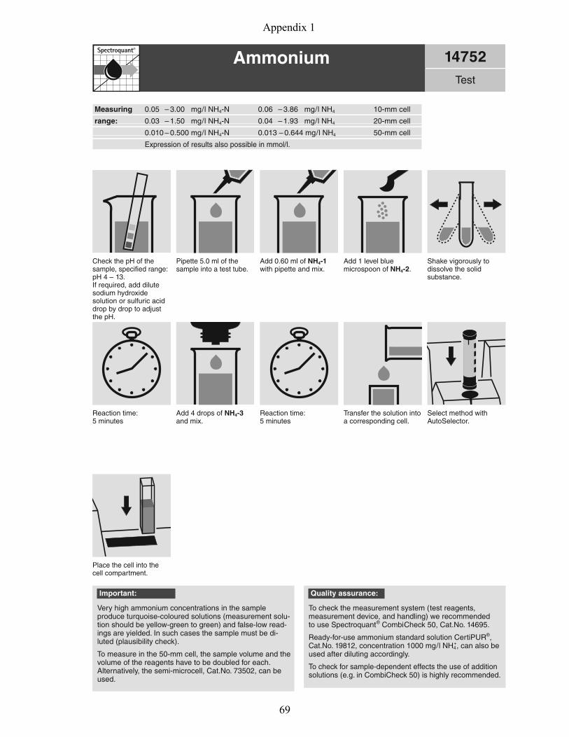
R

Measuring 0.05 – 3.00 mg/l NH4-N 0.06 – 3.86 mg/l NH4 10-mm cell

range: 0.03 – 1.50 mg/l NH4-N 0.04 – 1.93 mg/l NH4 20-mm cell

0.010 – 0.500 mg/l NH4-N 0.013 – 0.644 mg/l NH4 50-mm cell

Expression of results also possible in mmol/l.

Ammonium 14752Test

Add 4 drops of NH4-3 and mix.

Reaction time:5 minutes

Transfer the solution into a corresponding cell.

Select method with AutoSelector.

Place the cell into the cell compartment.

Pipette 5.0 ml of the sample into a test tube.

Add 0.60 ml of NH4-1 with pipette and mix.

Add 1 level bluemicrospoon of NH4-2.

Shake vigorously to dissolve the solid substance.


Check the pH of the sample, specified range:pH 4 – 13.If required, add dilute sodium hydroxide solution or sulfuric acid drop by drop to adjust the pH.

Important:

Very high ammonium concentrations in the sample produce turquoise-coloured solutions (measurement solu-tion should be yellow-green to green) and false-low read-ings are yielded. In such cases the sample must be di-luted (plausibility check).

To measure in the 50-mm cell, the sample volume and the volume of the reagents have to be doubled for each.Alternatively, the semi-microcell, Cat.No. 73502, can be used.

Quality assurance:

To check the measurement system (test reagents, measurement device, and handling) we recommended to use Spectroquant® CombiCheck 50, Cat.No. 14695.

Ready-for-use ammonium standard solution CertiPUR®, Cat.No. 19812, concentration 1000 mg/l NH4

+, can also be used after diluting accordingly.

To check for sample-dependent effects the use of addition solutions (e.g. in CombiCheck 50) is highly recommended.

Appendix 1

69

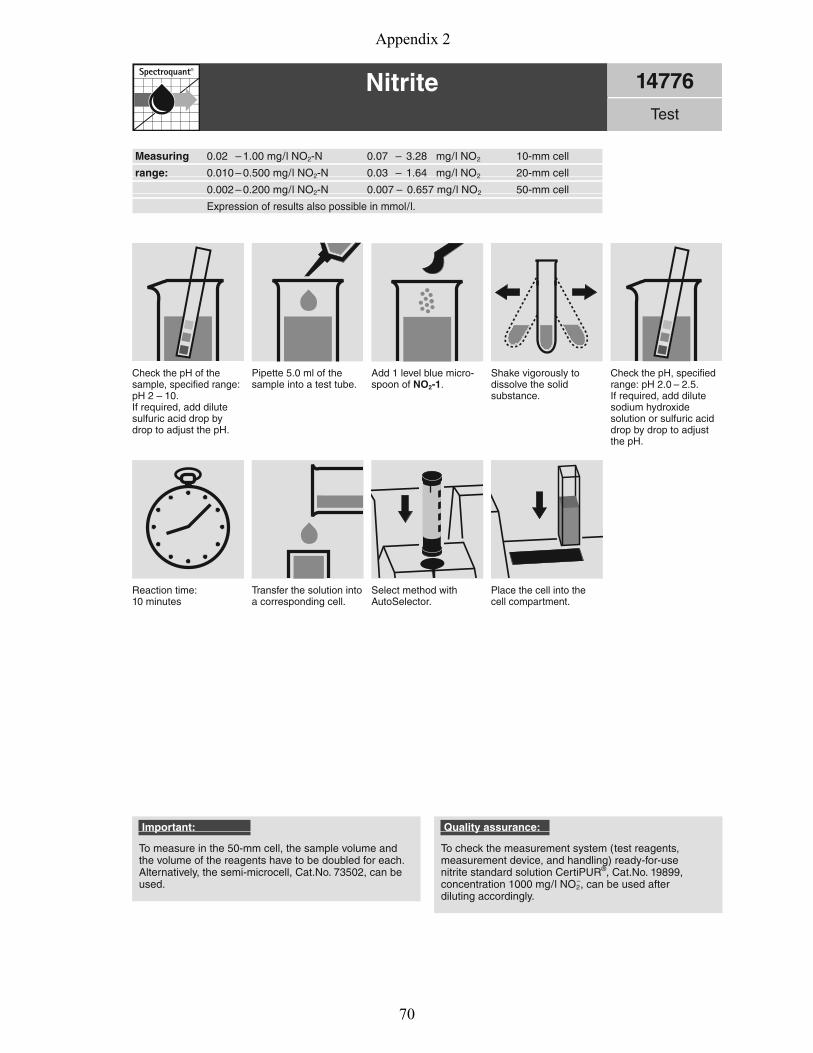
R

Check the pH, specified range: pH 2.0 – 2.5.If required, add dilute sodium hydroxide solution or sulfuric acid drop by drop to adjust the pH.

Pipette 5.0 ml of the sample into a test tube.

Nitrite 14776Test

Transfer the solution into a corresponding cell.


Place the cell into the cell compartment.

Quality assurance:

To check the measurement system (test reagents,measurement device, and handling) ready-for-use nitrite standard solution CertiPUR®, Cat.No. 19899, concentration 1000 mg/l NO2

–, can be used after diluting accordingly.

Shake vigorously to dissolve the solid substance.

Measuring 0.02 – 1.00 mg/l NO2-N 0.07 – 3.28 mg/l NO2 10-mm cell

range: 0.010 – 0.500 mg/l NO2-N 0.03 – 1.64 mg/l NO2 20-mm cell

0.002 – 0.200 mg/l NO2-N 0.007 – 0.657 mg/l NO2 50-mm cell


Add 1 level blue micro-spoon of NO2-1.


Check the pH of the sample, specified range:pH 2 – 10.If required, add dilute sulfuric acid drop by drop to adjust the pH.

Important:

To measure in the 50-mm cell, the sample volume andthe volume of the reagents have to be doubled for each.Alternatively, the semi-microcell, Cat.No. 73502, can be used.

Appendix 2

70

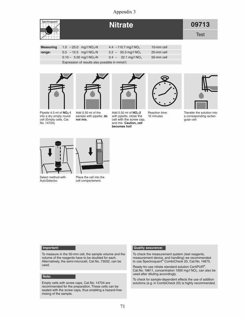
R

Nitrate 09713Test

Pipette 4.0 ml of NO3-1 into a dry empty round cell (Empty cells, Cat.No. 14724).

Transfer the solution into a corresponding rectan-gular cell.


Place the cell into the cell compartement.

Add 0.50 ml of NO3-2 with pipette, close the cell with the screw cap, and mix. Caution, cell becomes hot!

Measuring 1.0 – 25.0 mg/l NO3-N 4.4 – 110.7 mg/l NO3 10-mm cell

range: 0.5 – 12.5 mg/l NO3-N 2.2 – 55.3 mg/l NO3 20-mm cell

0.10 – 5.00 mg/l NO3-N 0.4 – 22.1 mg/l NO3 50-mm cell


Add 0.50 ml of the sample with pipette, do not mix.


Important:

To measure in the 50-mm cell, the sample volume and the volume of the reagents have to be doubled for each.Alternatively, the semi-microcell, Cat.No. 73502, can be used.

Quality assurance:

To check the measurement system (test reagents, measurement device, and handling) we recommended to use Spectroquant® CombiCheck 20, Cat.No. 14675.

Ready-for-use nitrate standard solution CertiPUR®, Cat.No. 19811, concentration 1000 mg/l NO3

–, can also be used after diluting accordingly.


Note:

Empty cells with screw caps, Cat.No. 14724 are recommended for the preparation. These cells can be sealed with the screw caps, thus enabling a hazard-free mixing of the sample.

Appendix 3

71

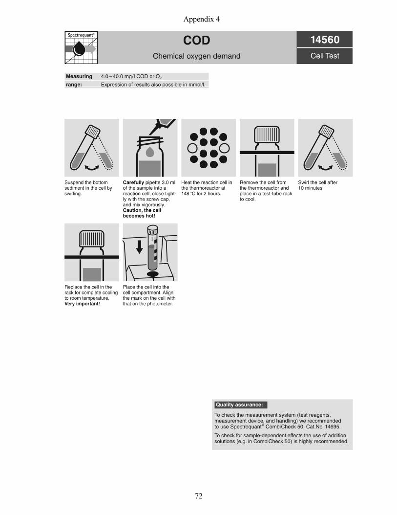
R

14560Cell Test

CODChemical oxygen demand

Quality assurance:

To check the measurement system (test reagents,measurement device, and handling) we recommended to use Spectroquant® CombiCheck 50, Cat.No. 14695.


Measuring 4.0 – 40.0 mg/l COD or O2

range: Expression of results also possible in mmol/l.

Place the cell into the cell compartment. Align the mark on the cell with that on the photometer.

Carefully pipette 3.0 ml of the sample into a reaction cell, close tight-ly with the screw cap, and mix vigorously. Caution, the cell becomes hot!

Suspend the bottom sediment in the cell by swirling.

Heat the reaction cell in the thermoreactor at 148 °C for 2 hours.

Remove the cell from the thermoreactor and place in a test-tube rack to cool.

Swirl the cell after 10 minutes.

Replace the cell in the rack for complete cooling to room temperature. Very important!

Appendix 4

72

Postboks 5003 NO-1432 Ås, Norway+47 67 23 00 00www.nmbu.no

Documents

Water Quality in RAS for Salmonids and Performance of MBBR