Embed Size (px)
Citation preview

Water for Wajir
Decision modeling for the Habaswein-Wajir Water Supply Project
in Northern Kenya
Eike Luedeling, Jan De Leeuw
World Agroforestry Centre, Nairobi, Kenya
August 2014

1
Water for Wajir – decision modeling for the Habaswein-Wajir
Water Supply Project in Northern Kenya
Contents Background ................................................................................................................................................... 3
Process .......................................................................................................................................................... 4
Modeling approach ....................................................................................................................................... 4
Major model elements ................................................................................................................................... 5
Stakeholders .............................................................................................................................................. 5
Costs .......................................................................................................................................................... 5
Benefits ..................................................................................................................................................... 6
Risks .......................................................................................................................................................... 7
Model implementation .............................................................................................................................. 7
Estimate elicitation and consolidation ...................................................................................................... 8
Post processing.......................................................................................................................................... 9
Consideration of risks ............................................................................................................................... 9
Results ......................................................................................................................................................... 10
Residents of Wajir ................................................................................................................................... 10
Residents of Habaswein .......................................................................................................................... 13
Pipeline communities .............................................................................................................................. 16
Upstream areas ........................................................................................................................................ 17
Downstream areas ................................................................................................................................... 18
Donors ..................................................................................................................................................... 19
Water company ....................................................................................................................................... 20
Overall project benefits ........................................................................................................................... 23
Discussion ................................................................................................................................................... 27
Recommendations ....................................................................................................................................... 27
References ................................................................................................................................................... 28
Annex 1: Model details ............................................................................................................................... 30
Wajir, Habaswein and pipeline communities...................................................................................... 30
Upstream and downstream areas ......................................................................................................... 30
Water company ................................................................................................................................... 30
Donor .................................................................................................................................................. 30

2
Overall net present benefits from the project ...................................................................................... 31
Risks .................................................................................................................................................... 31
Sampling ............................................................................................................................................. 31
Varying values .................................................................................................................................... 31
Discounting ......................................................................................................................................... 32
Annex 2: Results from the Monte Carlo analysis for pipeline communities, upstream and downstream
areas ............................................................................................................................................................ 33
Annex 3: Estimates ..................................................................................................................................... 39
All-risks scenario .................................................................................................................................... 39
Cooperation scenario .............................................................................................................................. 48

3
Water for Wajir – decision modeling for the Habaswein-Wajir
Water Supply Project in Northern Kenya
Eike Luedeling, Jan De Leeuw
World Agroforestry Centre, Nairobi, Kenya
Background The city of Wajir in Northern Kenya, the capital of the county of the same name, has experienced rapid
population growth in recent decades. The city has so far never had a reliable supply of clean drinking
water or a sanitation system. To improve the situation, plans are currently considered to construct a water
pipeline from Habaswein, another locale in Wajir County that is about 110 km away (Figure 1).
Figure 1. Map of the study region showing the approximate course of the proposed pipeline.
In Habaswein, the Merti aquifer would be tapped and water abstracted and piped to Wajir. Even though
the Kenyan government and the Dutch donor ORIO stand ready to fund this undertaking, the project is
currently stalled for a number of reasons, including the delayed completion of various feasibility and

4
impact studies and because of resistance in Habaswein. Local residents fear that the pipeline would
undermine their own water supply and many therefore oppose the project. It is also not clear, which of the
various stakeholders would benefit or suffer from the intervention, and whether it is prudent for the donor
to invest in this pipeline.
With funding from the UK National Environment Research Council, the World Agroforestry Centre,
together with the Centre for Training and Integrated Research in ASAL Development (CETRAD, Kenya),
University College London (United Kingdom) and Acacia Water (The Netherlands), conducted this study
to make a business case for the pipeline project that considers all relevant costs, benefits and risks.
Process The project kicked off with a 1-day stakeholder workshop (November 4, 2013) that gathered around 30
people with an interest in the pipeline project. During this meeting, a smaller group of 8 experts was
formed that spent the next two days (November 5 and 6) delineating all important aspects of the business
case. This was followed by coding of the model by a decision analyst. Following a few rounds of
feedback that helped improve the model, estimates of the probability distributions of all uncertain
variables in the model were elicited from the experts. Expert estimates were consolidated into group
estimates. After some more refinement of the model, it was run as a Monte Carlo simulation (many model
runs with varying input values). Results were compiled and summarized in a first version of this report,
which was shared with the modeling team. After a further consultative workshop (May 26, 2014), during
which more feedback was elicited and following inclusion of results from detailed hydrological modeling,
final model runs were executed and this report updated to its current version.
Modeling approach In order to build a comprehensive business case model of the proposed project, all major costs and
benefits, as well as all risks to the project were first compiled and relationships between them identified.
In this step, the modeling team aimed at comprehensiveness – identifying all relevant variables – rather
than at a high level of mechanistic detail. Based on the relationships between variables, equations were
defined to translate the various variables into the net present benefits of the project. These are the sum of
all benefits minus the sum of all costs, while considering the various risks that are involved. Such
calculations were done separately for all major stakeholders. In order to adjust for the time preference of
the stakeholders – i.e. the fact that they value benefits less highly if they accrue far in the future – all
results were discounted using standard economic procedures.
For running the model, estimates of all uncertain variables were required. Such estimates were elicited
from the members of the modeling team, who were asked to provide confidence intervals or probability
distributions that represented their uncertainty about the variables. For instance, an estimator might state
that the risk of political interference is between 10 and 50%, with a 90% chance that the real value is in
this interval. Since most people are not initially very good at making such estimates, all team members
were subjected to calibration training. During this training they were introduced to a number of
techniques to help them accurately estimate their uncertainty. Once estimates from all team members had
been collected for all uncertain variables, the analyst consolidated these into probability distributions that
represented the team’s level of uncertainty.

5
Based on the resulting distributions, Monte Carlo simulations of the net benefits of the project were run.
In such simulations, outcomes are calculated with the model many times – in this case 10,000 times –
with slightly varying values for all input variables. The values are determined by randomly drawing
samples from the defined distributions. Each run of the model provides one estimate of net present
benefits, and the totality of all model runs generates a probability distribution of these outcomes that
illustrates the probabilities, with which the project results in net gains and losses. The distribution also
indicates the likely magnitude of these gains and losses.
While the outcome distribution already provides a useful result, it can be analyzed further to identify
high-value variables in the calculation. These are the key uncertainties that determine the outcome. It is
these variables that could be measured to reduce the uncertainty of the decision maker about likely
decision outcomes.
Where the above analysis already provides a clear idea of which decision alternative is preferable, a
recommendation can immediately be made. Where both gains and losses are possible, measurement of
high-value variables is often justified. Once such measurements have been taken, the simulation
procedure can be repeated, possibly followed by more measurements. It is likely that after a few such
rounds, a clearly preferable decision option emerges.
Major model elements
Stakeholders
Separate analyses were conducted for the following stakeholder groups to see who stands to benefit or
lose from the proposed project:
Residents of Wajir
Residents of Habaswein
Communities along the pipeline
Upstream communities
Downstream communities
Water company (charged with operating the system)
Donor consortium
Costs and benefits for all these stakeholders were considered in different model modules. These were
similar in structure for the residents of the two communities and along the pipeline, for whom the same
types of costs and benefits may arise. Upstream and downstream effects were modeled at a much
aggregated level only, with the option to add more detail if results indicated that this was warranted. For
the water company, particular attention was paid to profitability of the company as a business.
Costs
Costs considered in the model were mostly the costs of operating the system, as well as fees for water
purchases by residents. Negative environmental impacts were considered for the upstream and
downstream communities only. All cost items and the stakeholders to which they applied are listed in
Table 1.

6
Table 1. Cost categories considered in the model and stakeholders to which they were applied (X means that the
respective cost was considered for a stakeholder).
Cost category
Res
iden
ts o
f
Wa
jir
Res
iden
ts o
f
Ha
ba
swei
n
Res
iden
ts o
f
pip
elin
e
com
mu
nit
ies
Up
stre
am
are
as
Do
wn
stre
am
are
as
Wa
ter
com
pa
ny
Do
no
r
con
sort
ium
Initial investment - - - - - X X
Running costs and metering - - - - - X -
Salaries - - - - - X -
Repairs - - - - - X -
Aquifer monitoring - - - - - X -
Infrastructure maintenance - - - - - X -
Pipeline security - - - - - X -
Payments for ecosystem services X - - - - X -
Negative environmental impacts - - - X X - -
Expenses for water purchases X X X - - - -
Benefits
The water company stands to benefit mainly through sale of water to its customers in Wajir, Habaswein
and along the pipeline. Upstream and especially downstream communities may benefit from payments for
ecosystem services, but are otherwise unlikely to experience positive impacts from the intervention. The
residents of Wajir, Habaswein and along the pipeline are expected to receive a wide range of benefits,
mostly related to new economic opportunities and improved public health (Table 2).
Table 2. Benefit categories considered in the model and stakeholders to which they were applied (X means that the
respective benefit was considered for a stakeholder).
Cost category
Res
iden
ts o
f
Wa
jir
Res
iden
ts o
f
Ha
ba
swei
n
Res
iden
ts o
f
pip
elin
e
com
mu
nit
ies
Up
stre
am
are
as
Do
wn
stre
am
are
as
Wa
ter
com
pa
ny
Do
no
r
con
sort
ium
Reduced infant mortality X X X - - - -
Reduced costs for disease
treatment X X X - - - -
Higher productivity X X X - - - -
Job creation X X X - - - -
Higher investments X X X - - - -
Reduced brain drain X X X - - - -
Revenue from more demand for
local products and services X X X - - - -
Higher tax revenue X X X - - - -
Reduced reliance on shallow
wells X X X - - - -
Sanitation benefits X X X - - - -
Water during the dry season X X X - - - -
General livelihood improvement X X X - - - -
Revenue from water sales - - - - - X -
Revenue from PES - X - X X - -

7
Risks
A number of risk factors threaten the feasibility of the project or have potential to reduce its operational
efficiency. Residents and opinion leaders have concerns about the hydrological sustainability of the
project, i.e. they are worried that it may undermine the reliability of their own water supply, which has
historically been very stable. This perception has led to substantial risk of political interference and
unwillingness to cooperate in project development, constituting another risk factor. Some risks to the
project threaten to completely prevent the intervention from happening. Other risks may make the project
fail at some point in the future (e.g. salinity build-up). Other risk factors, particularly regional conflict or
poor maintenance, may lead to temporary failure of the system. The last risk category contains factors that
merely reduce the efficiency of the pipeline, either permanently or temporarily. Specifically, the
following risk factors were considered:
Factors that lead to immediate project cancellation:
Negative feasibility report
Water yield too low
Inadequate benefit sharing
Political interference
Factors that lead to cancellation later:
Wells run dry
Increasing water salinity
Oil development (raising the risks of wells running dry or turning saline)
Dam development (raising the risks of wells running dry or turning saline)
Factors that cause temporary failure of project benefits
Maintenance problems
Water price is too high
Regional conflict
Factors that reduce project performance from the beginning:
Poor project design
Factors that temporarily reduce project performance:
Poor maintenance and operation
Illegal abstractions
Lack of cooperation
Model implementation
Mathematically, all risks were organized into two factors. The first factor described whether any benefits
accrued in a given year. In the case of immediate project cancellation, this factor was set to zero for all

8
years; if cancellation occurred later, zeroes were inserted for all years that followed. For temporary
failure, only the respective year received a zero weight. All non-zero years received a factor value of 1.
The second factor was used to scale the benefits. This factor comprised all the performance-reducing
risks, which were considered by reducing the amount of benefits by a certain percentage. These
percentages were multiplied for all risks, producing an overall benefit-scaling factor with the following
form:
∏ , in which nRisks is the number of individual risks and
is the benefit reduction (ranging between 0 and 1) expected due to risk i.
The analysis was run over a 30-year time horizon. All benefits were multiplied by both risk factors for all
years and costs subtracted to produce annual project budgets. These were produced for each stakeholder
group separately. Stakeholder time preference was then considered by discounting future profits by a
user-specified (and uncertain) discount rate. The resulting annual values were then added to produce an
overall Net Present Value for the intervention. Finally, results for all stakeholders were summed and
overall net present benefits for the project calculated, in addition to the individual stakeholder results.
Details of the model are provided in an annex to this report.
Estimate elicitation and consolidation
All members of the modeling team were ‘calibrated’. This process involved instruction in techniques to
improve their capacity to estimate the state of their own uncertainty. Training participants also took a
series of estimation tests to gauge their initial skill level and track progress throughout the training.
Calibration training is a standard procedure developed by Hubbard Decision Research (Hubbard, 2014),
which has been shown to strongly increase people’s capacity to provide accurate estimates.
All calibrated estimators were asked to fill estimation spreadsheets, which contained all uncertain
variables in the model. For each variable, they provided the upper and lower bounds of their own 90%
confidence interval. They were also encouraged to specify the distribution type for each variable, though
most variables were ultimately assumed to be normally distributed.
All estimates were then processed into diagrams that illustrated the different ranges provided by the
estimators. Based on these diagrams, as well as some intuitive weighting, when certain estimators were
deemed more credible informants than others (e.g. European team members were likely not well informed
about local issues of Wajir County), consolidated team estimates were then prepared by the analyst. These
were used to run the Monte Carlo simulation. For selected variables, some co-variation was assumed in
sampling variables for the simulation. The water prices and the numbers of water users at Wajir,
Habaswein and the communities along the pipeline were set to be negatively correlated. This was entered
into the model by drawing random samples in such a way that the resulting distributions correlated with a
coefficient of determination (r) of approximately -0.7. In the ‘all risks’ scenario, the Payment for
Ecosystem Services rate charged to all water sales was assumed to be negatively correlated (r = -0.7) with
the risks of inadequate benefit sharing and political interference. These two risk factors were assumed to
be proportional (r = 1).

9
Post processing
The Monte Carlo simulation for the pipeline project, which included 10,000 model runs, produced 10,000
projected results. These 10,000 results were displayed in single histograms to provide a visual impression
of likely distribution of project outcomes. In addition, all outcomes for all stakeholders were statistically
related to all uncertain input variables using Partial Least Squares (PLS) regression (Wold, 1995; Wold et
al., 2001; Luedeling and Gassner, 2012). This procedure calculates the so-called ‘Variable Importance in
the Projection’ statistic for each variable. This measure is an expression of the extent to which variation in
the independent variables explains variation in the outcome. Plotting this metric for all variables allows
identification of the key uncertainties in the calculation whose reduction through measurement would
increase the certainty with which outcomes can be projected. In such plots, bars are shown in red, when
low values for the respective variable are associated with high values for project outcomes, and in green
when there was a positive relationship between the two.
Consideration of risks
There are two ways to look at the present study, which reflect on how risks must be considered. One
interpretation of this model is that it is a forecast of what is likely to happen. In that case, all risks must be
considered in the model, including the chance that the project is not implemented. To fill the stakeholder
desire for an evaluation of the technical feasibility and environmental and financial sustainability of the
pipeline, however, it makes more sense to exclude certain risk factors, such as the chance of political
interference, from the simulation runs. This is useful, because the study itself may sway opinions, and
various political tools may also be employed to improve stakeholder perceptions of the project (e.g.
awareness building or payments for ecosystem services). The model then fulfills the desire by decision-
makers to obtain as objective an overview as possible of the general desirability of the pipeline project, so
that political positions on the issue can be developed. Because of these two interpretations of the
modeling procedure, all simulations were therefore run with and without politics-related risk factors.

10
Results Separate results were produced for each stakeholder group: the residents of Wajir, Habaswein and the
communities along the pipeline, areas upstream and downstream, the donor consortium and the water
company. In general, when considering the entire spectrum of risks that were identified, the project
currently seems unlikely to succeed. This is not so much because the intervention is infeasible or would
not benefit the stakeholders, but rather because key stakeholders are opposed to the project idea and are
likely to interfere during the politicized decision making process or the implementation of the project.
This high risk is clearly visible in results for all stakeholders, many of whom are most likely to see neither
net benefits nor net costs from the intervention, when all risks are considered. When excluding all risks
related to contrasting and conflicting stakeholder perceptions, the outlook for the project becomes more
favorable, though substantial risks of losses remain for all stakeholders.
Residents of Wajir
When considering all risks of the project, residents of Wajir are likely to see neither net benefits not net
costs (41.7% of all simulation runs; Table 3). Thirty-four percent of runs resulted in a loss and 24.3% in a
net benefit from the project. Plausible losses (10% quantile) were up to 262.0 million USD, while
plausible benefits (90% quantile) ranged up to 112.4 million USD). The full distribution is shown in the
inset of Figure 2. The most influential variables responsible for the wide range of projected outcomes
were related to the cost of water, the number of water users and the valuation and extent of reductions in
infant mortality and the number of disease treatments needed for water-borne diseases (Figure 2). Poor
project design and trends in water revenue were also identified as important factors.
Table 3. Characteristics of the net present benefit distribution for the residents of Wajir, for the two risk consideration
scenarios.
All risks considered
Net present benefit quantiles (million USD)
0% 10% 25% 50% 75% 90% 100%
-1550.4 -262.0 -68.9 0.0 0.0 112.4 714.3
Chance (%) of
Mean net present benefit (million USD) loss zero Benefits
-40.9 34.0 41.7 24.3
Assuming no political obstacles
Net present benefit quantiles (million USD)
0% 10% 25% 50% 75% 90% 100%
-1315.5 -348.2 -176.6 -15.9 67.4 170.7 744.6
Chance (%) of
Mean net present benefit (million USD) loss zero Benefits
-62.8 53.6 5.9 40.5

11
Figure 2. Important factors that limit the precision of outcome projections for the residents of Wajir, for the scenario in
which all risks are considered, according to the Variable-Importance-in-the-projection statistic of Partial Least Squares
regression. Inset: Net present benefit (in USD) distribution for the residents of Wajir, considering all relevant risks.
Assuming that political obstacles can be cleared, the chance of zero net benefits was reduced to 5.9%
(Table 3). Net losses to the residents of Wajir remained more likely (53.6% chance) than net benefits
(40.5%). Plausible losses ranged up to 348.2 million USD, while plausible benefits up to a value of 170.7
million USD appeared possible. The full distribution is shown in the inset of Figure 3. Important
uncertainties worth reducing were related to water purchases and prices and the magnitude and valuation
of improvements in public health and infant mortality (Figure 3). Trends in water prices and the quality of
project design were also worth closer scrutiny.

12
Figure 3. Important factors that limit the precision of outcome projections for the residents of Wajir, assuming that all
political obstacles have been cleared, according to the Variable-Importance-in-the-projection statistic of Partial Least
Squares regression. Inset: Net present benefit (in USD) distribution for the residents of Wajir, assuming that all political
obstacles have been cleared.

13
Residents of Habaswein
Also for the residents of Habaswein, the high chance of project failure made it likely that no net benefits
or costs would arise (41.7%; Table 4). Among the remaining model runs, the chance of net benefits
(51.3%) outweighed the chance of net costs (7.0%). The range of plausible outcomes (10-90% quantiles)
was 0 to 71.7 million USD. The full distribution for this scenario is shown in the inset of Figure 4.
Influential variables in the model were the number and valuation of additionally surviving infants, the
amount of water purchased by residents from the water company and the number and valuation of disease
treatments that will no longer be necessary (Figure 4). As was the case for Wajir, the risk of political
interference, inadequate benefit sharing and the chance of poor project design were also major sources of
uncertainty. Productivity gains at Habaswein and the rate of Payments for Environmental Services, which
are partly assumed to benefit Habaswein, also had important impacts on projected outcomes. Finally, the
number of water users was also identified as important.
Table 4. Characteristics of the net present benefit distribution for the residents of Habaswein, for the two risk
consideration scenarios.
All risks considered
Net present benefit quantiles (million USD)
0% 10% 25% 50% 75% 90% 100%
-116.5 0.0 0.0 2.6 37.7 71.7 323.7
Chance (%) of
Mean net present benefit (million USD) loss zero benefits
22.4 7.0 41.7 51.3
Assuming no political obstacles
Net present benefit quantiles (million USD)
0% 10% 25% 50% 75% 90% 100%
-102.1 -1.5 8.6 30.5 60.0 95.0 276.1
Chance (%) of
Mean net present benefit (million USD) loss zero benefits
38.7 11.0 5.9 83.0
14
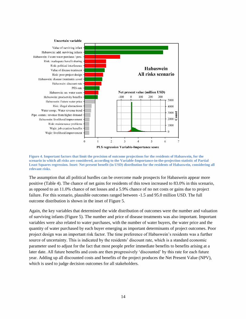
Figure 4. Important factors that limit the precision of outcome projections for the residents of Habaswein, for the
scenario in which all risks are considered, according to the Variable-Importance-in-the-projection statistic of Partial
Least Squares regression. Inset: Net present benefit (in USD) distribution for the residents of Habaswein, considering all
relevant risks.
The assumption that all political hurdles can be overcome made prospects for Habaswein appear more
positive (Table 4). The chance of net gains for residents of this town increased to 83.0% in this scenario,
as opposed to an 11.0% chance of net losses and a 5.9% chance of no net costs or gains due to project
failure. For this scenario, plausible outcomes ranged between -1.5 and 95.0 million USD. The full
outcome distribution is shown in the inset of Figure 5.
Again, the key variables that determined the wide distribution of outcomes were the number and valuation
of surviving infants (Figure 5). The number and price of disease treatments was also important. Important
variables were also related to water purchases, with the number of water buyers, the water price and the
quantity of water purchased by each buyer emerging as important determinants of project outcomes. Poor
project design was an important risk factor. The time preference of Habaswein’s residents was a further
source of uncertainty. This is indicated by the residents’ discount rate, which is a standard economic
parameter used to adjust for the fact that most people prefer immediate benefits to benefits arising at a
later date. All future benefits and costs are then progressively ‘discounted’ by this rate for each future
year. Adding up all discounted costs and benefits of the project produces the Net Present Value (NPV),
which is used to judge decision outcomes for all stakeholders.

15
Figure 5. Net present benefit (in USD) distribution for the residents of Habaswein, assuming that all political obstacles
have been cleared.

16
Pipeline communities
For communities along the pipeline, chances of project failure were the same as for Wajir and Habaswein.
For these settlements, the chance of benefits outweighed the chance of losses for both scenarios (Table 5).
Overall the chance of benefiting from the project was 43.0% for the all-risks scenario and 70.3% for the
no-obstacles scenario. Distributions of likely outcomes for the pipeline communities had the same shape
as for Habaswein because of similar cost and benefit structures. Also for pipeline communities, number
and valuation of surviving infants and disease treatments, questions about the basic economics of water
sales (number of customers, price) and the quality of project design were of importance. Inadequate
benefit sharing and political interference emerged as important uncertain risk factors. Figures for the
pipeline communities are provided in the annex.
Table 5. Characteristics of the net present benefit distribution for the residents of communities along the pipeline, for the
two risk consideration scenarios.
All risks considered
Net present benefit quantiles (million USD)
0% 10% 25% 50% 75% 90% 100%
-88.9 -6.1 0.0 0.0 14.8 35.6 174.3
Chance (%) of
Mean net present benefit (million USD) loss zero benefits
8.4
15.3 41.7 43.0
Assuming no political obstacles
Net present benefit quantiles (million USD)
0% 10% 25% 50% 75% 90% 100%
-119.9 -13.8 0.0 10.7 28.1 48.6 222.3
Chance (%) of
Mean net present benefit (million USD) loss zero benefits
14.6
23.8 5.9 70.3

17
Upstream areas
Upstream areas were not expected to be much affected by the proposed intervention, but they were
included in the model because some impacts might be possible. When the risk of project failure due to
political factors was included, losses (49.7%) were about equally likely as gains (48.4%; Table 6). When
no political obstacles remained, the chance of benefits (78.9%) clearly outweighed the chance of losses
(20.7%). Important variables were mostly related to Payments for Ecosystem Services (PES), which were
assumed to be financed through a levy on water sales. It therefore depended on the share of total collected
PES going to upstream areas and the rate of the PES levy. Since most water revenue and therefore PES
payments would be collected in Wajir, water purchases and water price in Wajir were also important.
Important uncertain risk factors were the chance of political interference, inadequate benefit sharing and
poor project design. Habaswein’s PES share also emerged as an uncertainty, because a higher proportion
of PES revenue allocated to Habaswein would reduce the payments to upstream areas. Finally, the
environmental impact of the intervention on upstream areas was one of the key uncertainties. Figures for
upstream areas are shown in the annex.
Table 6. Characteristics of the net present benefit distribution for upstream areas, for the two risk consideration
scenarios.
All risks considered
Net present benefit quantiles (million USD)
0% 10% 25% 50% 75% 90% 100%
-0.5 -0.2 -0.1 0.0 0.3 0.7 4.2
Chance (%) of
Mean net present benefit (million USD) loss zero benefits
0.1 49.7 1.9 48.4
Assuming no political obstacles
Net present benefit quantiles (million USD)
0% 10% 25% 50% 75% 90% 100%
-1.0 -0.1 0.0 0.2 0.5 0.8 4.6
Chance (%) of
Mean net present benefit (million USD) loss zero benefits
0.3 20.7 0.4 78.9
18
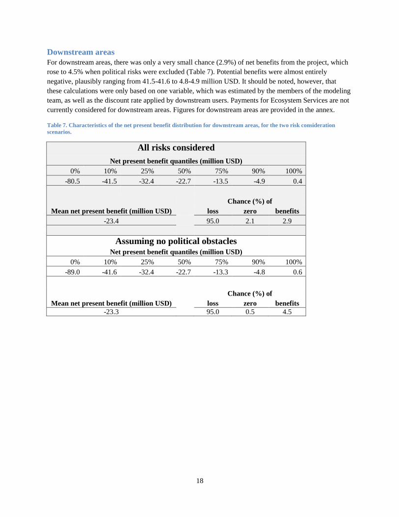
Downstream areas
For downstream areas, there was only a very small chance (2.9%) of net benefits from the project, which
rose to 4.5% when political risks were excluded (Table 7). Potential benefits were almost entirely
negative, plausibly ranging from 41.5-41.6 to 4.8-4.9 million USD. It should be noted, however, that
these calculations were only based on one variable, which was estimated by the members of the modeling
team, as well as the discount rate applied by downstream users. Payments for Ecosystem Services are not
currently considered for downstream areas. Figures for downstream areas are provided in the annex.
Table 7. Characteristics of the net present benefit distribution for downstream areas, for the two risk consideration
scenarios.
All risks considered
Net present benefit quantiles (million USD)
0% 10% 25% 50% 75% 90% 100%
-80.5 -41.5 -32.4 -22.7 -13.5 -4.9 0.4
Chance (%) of
Mean net present benefit (million USD) loss zero benefits
-23.4 95.0 2.1 2.9
Assuming no political obstacles
Net present benefit quantiles (million USD)
0% 10% 25% 50% 75% 90% 100%
-89.0 -41.6 -32.4 -22.7 -13.3 -4.8 0.6
Chance (%) of
Mean net present benefit (million USD) loss zero benefits
-23.3 95.0 0.5 4.5
19
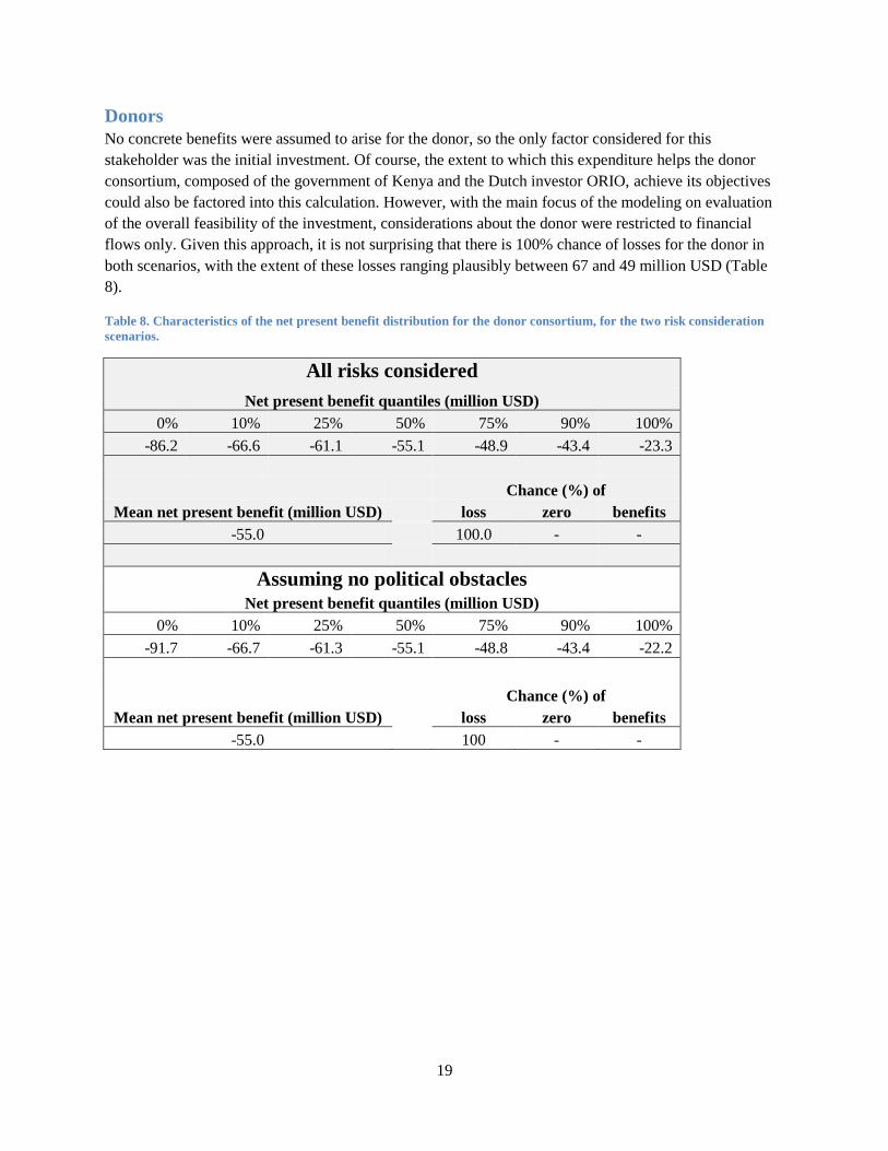
Donors
No concrete benefits were assumed to arise for the donor, so the only factor considered for this
stakeholder was the initial investment. Of course, the extent to which this expenditure helps the donor
consortium, composed of the government of Kenya and the Dutch investor ORIO, achieve its objectives
could also be factored into this calculation. However, with the main focus of the modeling on evaluation
of the overall feasibility of the investment, considerations about the donor were restricted to financial
flows only. Given this approach, it is not surprising that there is 100% chance of losses for the donor in
both scenarios, with the extent of these losses ranging plausibly between 67 and 49 million USD (Table
8).
Table 8. Characteristics of the net present benefit distribution for the donor consortium, for the two risk consideration
scenarios.
All risks considered
Net present benefit quantiles (million USD)
0% 10% 25% 50% 75% 90% 100%
-86.2 -66.6 -61.1 -55.1 -48.9 -43.4 -23.3
Chance (%) of
Mean net present benefit (million USD) loss zero benefits
-55.0 100.0 - -
Assuming no political obstacles
Net present benefit quantiles (million USD)
0% 10% 25% 50% 75% 90% 100%
-91.7 -66.7 -61.3 -55.1 -48.8 -43.4 -22.2
Chance (%) of
Mean net present benefit (million USD) loss zero benefits
-55.0 100 - -

20
Water company
Profitability for the water company of operating the pipeline may be the most important determinant of
project feasibility. Risks to this are quite high in the all-risks scenario, which indicated a 51.4% chance of
losses (Table 9). Due to the model structure, some losses were incurred even when the project failed.
When political risks were excluded, the chance of failure dropped to 21.0%, as opposed to a chance of
79.0% that the company would generate a profit. Plausible profits and losses were substantial in both
scenarios. In the all-risks scenario, net returns ranged from -109.3 to 447.7 million USD (10% to 90%
quantile), while the outlook in the no-obstacles scenario was brighter at -62.3 to 564.7 million USD. The
full distribution of projected outcomes for the all-risks scenario is shown in the inset of Figure 6 and for
the no-obstacles scenario in the inset of Figure 7.
Table 9. Characteristics of the net present benefit distribution for the water company, for the two risk consideration
scenarios.
All risks considered
Net present benefit quantiles (million USD)
0% 10% 25% 50% 75% 90% 100%
-755.7 -109.3 -88.3 -15.0 227.7 447.7 2000.9
Chance (%) of
Mean net present benefit (million USD) loss zero benefits
95.6 51.4 - 48.6
Assuming no political obstacles
Net present benefit quantiles (million USD)
0% 10% 25% 50% 75% 90% 100%
-866.0 -62.3 26.3 182.1 370.0 564.7 2165.9
Chance (%) of
Mean net present benefit (million USD) loss zero benefits
227.5 21.0 - 79.0
For the water company, key uncertainties were related mainly to their main market for water in Wajir,
most notably the amount of water likely to be sold to each customer, the water price and the trend in
water revenue (Figure 6). In the all-risks scenario, the risk of political interference, inadequate benefit
sharing and poor project design were major risk factors. The rate of Payments for Ecosystem Services
was also an important factor. Interestingly a higher PES rate, which at the surface might look like a loss to
the water company, was related to high profits, because these payments were assumed to ease political
resistance to the project and foster collaboration. Further variables worth measuring were the salaries paid
to water company employees, running costs of the company and the base risks of drying wells and
increasing salinity. In the no-obstacles scenario, the key uncertainties were similar to the all-risks
scenario, except for the political risks, which were excluded (Figure 7).

21
Figure 6. Important factors that limit the precision of outcome projections for the water company, for the scenario in
which all risks are considered, according to the Variable-Importance-in-the-projection statistic of Partial Least Squares
regression. Inset: Net present benefit (in USD) distribution for the water company, considering all relevant risks.

22
Figure 7. Important factors that limit the precision of outcome projections for the water company, assuming that all
political obstacles have been cleared, according to the Variable-Importance-in-the-projection statistic of Partial Least
Squares regression. Inset: Net present benefit (in USD) distribution for the water company, assuming that all political
obstacles have been cleared.

23
Overall project benefits
Adding up all net present benefits for all stakeholders provided an illustration of the overall desirability,
expressed by a high Net Present Value of the project, of constructing the pipeline. It should be noted here
that the investment is considered to aim at maximizing overall benefits for all stakeholders rather than
those of the investor only. In fact, according to the analyst’s understanding of the planned investment, the
investor is certain to make a loss, which, however, may be appropriate in a government measure or
benevolent development project.
When considering all risks, the project was more likely to result in a net loss (55.9% chance) than a net
benefit (44.1%; Table 10). The 10% quantile of the distribution, which can be considered the poorest
plausible outcome, was equivalent to a loss of 192.3 million USD. The highest plausible result, however,
the 90% quantile, was a net benefit of 302.2 million USD. The full distribution is shown in the inset of
Figure 8, which clearly shows the large spike in the distribution that is related to the high chance of
project failure. In most such cases, some costs are incurred, shifting the distribution towards negative
numbers.
As for several of the stakeholders, the value of a surviving infant was the most influential uncertainty in
the model (Figure 8). This was followed by the extent to which poor project design reduced system
performance and the number of additional infants that survive in Wajir. The value of a disease treatment
was also identified as influential. Among the top 8 variables were 3 that were related to political will: the
risk of political interference, inadequate benefit sharing and the Payment for Ecosystem Services rate
(which was correlated to the political risk factors). This finding underscores the necessity to build
consensus on the project among all stakeholders and ensure that they all perceive the intervention as
beneficial.
Table 10. Characteristics of the net present benefit distribution for the project, for the two risk consideration scenarios.
All risks considered
Net present benefit quantiles (million USD)
0% 10% 25% 50% 75% 90% 100%
-403.6 -192.3 -166.3 -52.8 142.1 302.2 1180.2
Chance (%) of
Mean net present benefit (million USD) loss zero benefits
7.2 55.9 - 44.1
Assuming no political obstacles
Net present benefit quantiles (million USD)
0% 10% 25% 50% 75% 90% 100%
-533.3 -115.9 -5.3 121.0 259.6 404.8 1275.6
Chance (%) of
Mean net present benefit (million USD) loss zero benefits
139.9 25.9 - 74.1

24
Further important variables were the discount rates of the water company and the residents of Wajir, the
downstream environmental impacts, the number of disease treatments that will no longer be necessary in
Wajir and the water company’s salaries and running costs. The size of the initial investment by the donors
also emerged as an important variable, along with losses due to illegal abstractions or poor maintenance.
Finally, reduction in infant mortality in Habaswein was also important.
Figure 8. Important factors that limit the precision of outcome projections for the overall project, for the scenario in
which all risks are considered, according to the Variable-Importance-in-the-projection statistic of Partial Least Squares
regression. Inset: Net present benefit (in USD) distribution for the overall project, considering all relevant risks.
Prospects for the project were much better under the assumption that political obstacles can be removed.
The chance of net benefits from the intervention improved to 74.1%, as opposed to a chance of loss of
25.9%. The range of plausible outcomes was -115.9 to 404.8 million USD, indicating that substantial
gains are possible, but there is also the chance of high losses. The full distribution is shown in the inset of
Figure 9. With the political risks removed, the value of a surviving infant remained the key uncertainty,
followed by the impacts of poor project design and the number of additional surviving infants in Wajir
(Figure 9). The value of disease treatment followed, along with the discount rate applied by residents of
Wajir. Next in importance came the number of saved disease treatments in Wajir, the number of

25
additional surviving infants in Habaswein, the losses from illegal abstractions and poor maintenance and
the salaries paid by the water company.
Figure 9. Important factors that limit the precision of outcome projections for the overall project, assuming that all
political obstacles have been cleared, according to the Variable-Importance-in-the-projection statistic of Partial Least
Squares regression. Inset: Net present benefit (in USD) distribution for the overall project, assuming that all political
obstacles have been cleared.
Visualization of projected outcome distributions for all stakeholder groups indicated that none of the two
scenarios provided unambiguous certainty about either positive or negative outcomes of the project. The
only exception was the financial prospect of the donor (Figure 10). There was thus substantial uncertainty
about the desirability of the Habaswein-Wajir Water Supply project for all stakeholders.

26
Figure 10. Overview of projected outcome distributions for all stakeholders for both risk consideration scenarios.

27
Discussion Given the current state of uncertainty, and the current political climate, the proposed project is very risky,
with plausible outcomes varying widely for all stakeholders (Figure 10). Considering estimates about the
risk of political interference and related variables, the chance of project failure is very high, possibly too
high for most investors. At the moment, political resistance comes mainly from the direction of
Habaswein, whose inhabitants are concerned about the sustainability of their water resources. This
resistance stands in contrast to the relatively small hydrological risks identified by the hydrological
studies that accompanied this assessment. In fact, when weighing all evidence and considering the
possibility that the town of Habaswein could be compensated through a PES scheme, the likelihood that
the pipeline project would generate net benefits was actually higher for Habaswein than for Wajir, where
water prices are expected to be quite a bit higher. So it seems possible that political resistance can be
overcome, which may be an essential step that must be undertaken, before the project can move forward.
In designing the details of this project, attention must be paid to fair sharing of benefits. The perception
that water will be taken away from Habaswein without fair compensation has already interfered with the
planning process. The importance of variables related to this issue was evident in many of the stakeholder
models. It will also be important to conduct environmental impact assessments on areas upstream and
downstream from Habaswein. These impacts emerged as key uncertainties for some stakeholders.
The uncertainty that will be hardest to address might be the valuation of a surviving infant. While this is
obviously a delicate and ethically charged judgment, it is critical for evaluating whether this project is
worth pursuing from the perspective of society as a whole. However, social benefits that are difficult to
quantify in an uncontroversial manner are not important for the cost-benefit considerations of the water
company. Our analysis revealed that even without political risk this project remains risky from the
perspective of the water company. This is worrying, because profitability of the water company is a major
factor determining the sustainability of the benefits of the project. The risk of bankruptcy of the water
company undermines this sustainability. The risk of negative returns of the water company is the result of
high uncertainties in a number of variables: the volume of water purchased and the price paid for the
water are the most important ones. Adequate pre-project market surveys on the demand and willingness to
pay for water could reduce these uncertainties and produce gains in certainty about project outcomes for
the water company. We propose undertaking additional research on these two and a number of other
variables, which have the largest influence on the current uncertainty around the financial outcomes for
the water company.
Recommendations The analysis clearly showed that this project involves substantial risks, which at present make it difficult
to decide whether this project will generate net benefits or losses. Targeted measurements, along with
modifications to the project design, could add clarity.
In terms of measurements, attention should be paid to infant mortality and water-borne diseases. This
analysis had no concrete data on these issues, except some official statistics on current infant mortality. In
particular, estimates about the reduction in diseases and the number of additional surviving infants were
highly uncertain. Precision could be added by investigating the infection pathways for water-borne
diseases and the causal factors for infant mortality in the particular context of Wajir County. This should

28
help with estimates of how the pipeline project is likely to affect both issues in the future. An evaluation
of the treatment costs for water-borne diseases should also be conducted. This should be easily achievable
by interviewing local health professionals. The greatest benefit-related uncertainty, which affected
outcomes for several stakeholders, was the value that a human life has to whoever makes the decision
about proceeding with this project. The current 90% confidence interval in the model is 200 to 100,000
USD. While it may be impossible to find a precise uncontroversial number for this variable, it may
nevertheless be possible to reduce this range.
We recommend one measurement that did not emerge as a key uncertainty but would likely contribute to
reducing political resistance to the project. The hydrological modeling showed only a small chance of
wells running dry but a greater chance that salinity might intrude into the aquifer from below the
freshwater layer. A relatively inexpensive test borehole into the deeper layers of the aquifer would help
clarify this issue and possibly contribute to overcoming political resistance.
Regarding project design, two issues emerged as important. Poor project design was identified as one of
the major risks to project success. The importance of doing adequate planning at the beginning of the
implementation phase cannot be overemphasized. Furthermore, activities to build consensus around the
intervention and ensure that all stakeholders approve of the intervention is critical. Payments for
Environmental Services were included in the model, but other benefit-sharing mechanisms, as well as
awareness-raising measures, should also be explored. While not considered as an option in the present
model, financial compensation of downstream areas for potentially negative environmental impacts could
also be considered. At present, downstream water users are the only clear losers of the intervention. Since
they would not strictly provide an environmental service to the project, they are not currently included in
the PES scheme, but project planners may consider adding damage compensation measures to the project
design.
Acknowledgment We acknowledge funding for this work by the UK National Environment Research Council and support
from the Cooperative Research Program on Water Land and Ecosystems (WLE) of the CGIAR.
Furthermore we are grateful to all members of the modeling team and to all participants of our workshops
for invaluable insights into the pipeline project.
References Hubbard, D.W., 2014. How to Measure Anything - Finding the Value of Intangibles in Business. Wiley.
Luedeling, E. and Gassner, A., 2012. Partial Least Squares regression for analyzing walnut phenology in
California. Agricultural and Forest Meteorology, 158: 43-52.
Wold, S., 1995. PLS for multivariate linear modeling. In: H. van der Waterbeemd (Editor), Chemometric
methods in molecular design: methods and principles in medicinal chemistry. Verlag-Chemie,
Weinheim, Germany, pp. 195-218.
Wold, S., Sjostrom, M. and Eriksson, L., 2001. PLS-regression: a basic tool of chemometrics. Chemom.
Intell. Lab. Syst., 58(2): 109-130.

29

30
Annex 1: Model details
Wajir, Habaswein and pipeline communities
Model modules for these three communities were identical. Benefits at all sites were derived by adding up
the following individual benefits: Reduced infant mortality, reduced costs for disease treatment, higher
productivity, job creation, higher investments, reduced brain drain, revenue from more demand for local
products and services, higher tax revenue, reduced reliance on shallow wells, sanitation benefits, water
during the dry season, general livelihood improvement (also listed earlier in the report). Payments for
Ecosystem Services (PES), i.e. availing water to Wajir, were considered for Habaswein. PES were
calculated as described below in the water company section. The option of PES payments for the other
communities was also built into the model, even though such payments are unlikely. Where model users
do not expect such payments to happen, the respective uncertain variable can be set to zero.
On the cost side, only the costs for purchasing water were considered. These were derived by multiplying
the number of water users, the amount of water purchased per person and the future water price. Since
people of these locations already purchase some water, often in bottles or jerry cans, the current water
price and consumption rate was also estimated, multiplied by the number of water users and subtracted
from the water costs. All costs and benefits were discounted to account for people’s time preference (see
below).
Upstream and downstream areas
The possibility was considered that downstream and upstream areas might experience negative impacts
from the project. This was not so much based on hydrological considerations, but entered the model as a
stand-alone estimate of the costs of damage that could possibly be caused. Revenues for both stakeholder
groups arose exclusively from PES. These payments were introduced, because the project might benefit
from certain management measures to conserve water in the upstream areas and extraction of water at
Habaswein could possibly affect development prospects downstream. PES payments are meant to
compensate for these costs or foregone profits.
Water company
For the water company, benefits arose exclusively through the sale of water. This resulted from simple
summation of the water costs paid by the three client stakeholders (Wajir, Habaswein and the
communities along the pipeline). Out of these revenues, a certain percentage was extracted to be used for
PES. These funds were distributed among all other stakeholders according to a weighting system
specified by the analyst (as uncertain variables).
On the cost side, a number of cost items were considered: Initial investment costs, running costs (incl.
metering), salaries, repairs, costs of aquifer monitoring, infrastructure maintenance, pipeline security,
costs incurred through waste of water and costs for wildlife conservation.
Donor
On the side of the donor, assumed to be a consortium of the Government of Kenya and the Dutch
company ORIO, only the initial investment costs were factored into the calculations.

31
Overall net present benefits from the project
The overall costs and benefits were derived by adding up all stakeholder benefits and subtracting costs to
all stakeholders. Risks were considered as described in the risk section below and all values were
discounted as outlined in the discounting section (also below).
Risks
Risks were considered in two different ways: through a project success factor and through a benefit
scaling factor.
Project success factor
The project success factor could only assume two values for a given year: zero and one. Its effect was that
it could set the benefits arising from the project to zero for any year, if the project suffered from
permanent or temporary failure.
Different risks had different effects on this factor. Risks such as a negative feasibility report, inadequate
water yield or political interference set the project success factor to zero for all years, meaning that no
benefits arise at all. Other risks, such as salinity increases or drying wells led the project success factor to
be set to zero for all years, starting in the year that the problem first arose. These two risks were expressed
by a base risk, to which a risk enhancement component was added. This component depended on the
development of oil or dam projects in the region, which was specified by a probability estimate. Finally,
temporary failure, which may be caused by regional conflict or lack of cooperation, led to the project
success factor to be set to zero for individual years only.
Benefit scaling factor
The benefit scaling factor was used to reduce the amount of benefits generated by the project, either
permanently or temporarily. It took the shape of a factor, ranging between 0 and 1, with which all benefits
were multiplied. Poor project design led to a permanent reduction in revenues, implemented by an
adjustment of the benefit scaling factor by a fixed amount in all years. Other factors were variable,
including poor maintenance or illegal abstractions, which were applied to different extents in each year.
Sampling
All uncertain variables were sampled from user-specified distributions. In most cases, these were normal
distributions characterized by 90% confidence intervals. A range of other distribution types could also be
specified but were rarely chosen by the estimators.
For some variables, co-variation was introduced. This was motivated by the realization that, e.g., the price
of something and the demand for it are normally not independent but follow some sort of negative
correlation. Consequently, the option to correlate variables was built into the algorithms, with users
having to specify the variables that were to co-vary, the confidence interval for each variable and the
desired coefficient of correlation (R2). This function currently only works for normally distributed
variables.
Varying values
For most variables, it is unreasonable to expect exactly the same value for each year of the simulation. A
value varying function was therefore introduced, which required as inputs the mean expected value for a
given variable and an estimate of its coefficient of variation. From these numbers, a time series that

32
included a measure of random variation was generated. This function also included the option to
introduce absolute or relative trends in the data, around which annual values varied. This function was
applied to the majority of variables in the model.
Discounting
It is common practice in economic analyses to discount costs and benefits that arise in the future by a
certain percentage for each year. This is motivated by the realization that most people and most
businesses prefer immediate returns over those that arise in the future. Discounting was applied to all
costs and benefits for all stakeholders, according to discount rates specified (as uncertain distributions) by
the estimators.

33
Annex 2: Results from the Monte Carlo analysis for pipeline communities,
upstream and downstream areas
Figure 11. Important factors that limit the precision of outcome projections for the residents of the communities along the
pipeline, for the scenario in which all risks are considered, according to the Variable-Importance-in-the-projection
statistic of Partial Least Squares regression. Inset: Net present benefit (in USD) distribution for the residents of the
communities along the pipeline, considering all relevant risks.

34
Figure 12. Important factors that limit the precision of outcome projections for upstream areas, assuming that all political
obstacles have been cleared, according to the Variable-Importance-in-the-projection statistic of Partial Least Squares
regression. Inset: Net present benefit (in USD) distribution for the residents of the communities along the pipeline,
assuming that all political obstacles have been cleared.

35
Figure 13. Important factors that limit the precision of outcome projections for upstream areas, for the scenario in which
all risks are considered, according to the Variable-Importance-in-the-projection statistic of Partial Least Squares
regression. Inset: Net present benefit (in USD) distribution for upstream areas, considering all relevant risks.

36
Figure 14. Important factors that limit the precision of outcome projections for upstream areas, assuming that all political
obstacles have been cleared, according to the Variable-Importance-in-the-projection statistic of Partial Least Squares
regression. Inset: Net present benefit (in USD) distribution for upstream areas, assuming that all political obstacles have
been cleared.

37
Figure 15. Important factors that limit the precision of outcome projections for downstream areas, for the scenario in
which all risks are considered, according to the Variable-Importance-in-the-projection statistic of Partial Least Squares
regression. Inset: Net present benefit (in USD) distribution for downstream areas, considering all relevant risks.

38
Figure 16. Important factors that limit the precision of outcome projections for downstream areas, assuming that all
political obstacles have been cleared, according to the Variable-Importance-in-the-projection statistic of Partial Least
Squares regression. Inset: Net present benefit (in USD) distribution for downstream areas, assuming that all political
obstacles have been cleared.

39
Annex 3: Estimates
All-risks scenario
Variable Description
Lower
bound
Upper
bound
Distrib-
ution* general variables
n_years number of years to run simulation 30 30 constant
cost_CV coefficients for introducing annual variation 10 15 pos_normal
benefit_CV coefficients for introducing annual variation 10 20 pos_normal
general_CV coefficients for introducing annual variation 10 15 pos_normal
general benefit valuation
value_of_surviving_infant How much should a avoided infant death be valued at? 200 100,000 pos_normal
value_of_disease_treatment How much does a treatment for water-borned disease cost? 3 300 pos_normal
future_water_price_m3_Habaswein
Price of a m3 of water in the project in Habaswein with the
project 1 5 correlated
future_water_price_m3_Wajir
Price of a m3 of water in the project in Wajir with the
project 1 20 correlated
future_water_price_m3_pipeline_com
munities
Price of a m3 of water in the project in along the pipeline
with the project 1 10 correlated
present_water_price_m3_Habaswein
Price of a m3 of water in the project in Habaswein at
present 5 20 normal
present_water_price_m3_Wajir Price of a m3 of water in the project in Wajir at present 5 20 normal
present_water_price_m3_pipeline_com
munities
Price of a m3 of water in the project in along the pipeline at
present 5 20 normal
Wajir_water_users Number of water users in Wajir 80,000 300,000 correlated
Habaswein_water_users Number of water users in Habaswein 20,000 100,000 correlated
Pipeline_communities_water_users
Number of water users in the communities along the
pipeline 1,500 50,000 correlated
Wajir_present_water_purchase_per_pe
rson_day_l Water purchase per person per day in Wajir at present 10 20 pos_normal

40
Variable Description
Lower
bound
Upper
bound
Distrib-
ution*
Habaswein_present_water_purchase_p
er_person_day_l Water purchase per person per day in Habaswein at present 10 20 pos_normal
Pipeline_communities_present_water_
purchase_per_person_day_l
Water purchase per person per day in communities along
the pipeline at present 10 20 pos_normal
Wajir_future_water_purchase_per_per
son_day_l
Water purchase per person per day in Wajir with the
project 20 80 pos_normal
Habaswein_future_water_purchase_pe
r_person_day_l
Water purchase per person per day in Habaswein with the
project 20 80 pos_normal
Pipeline_communities_future_water_p
urchase_per_person_day_l
Water purchase per person per day in communities along
the pipeline with the project 20 80 pos_normal
water_revenue_trend Water cost change trend (integrates price and #users; in %) 2 5 pos_normal
water_tax_rate Tax rate on water sales 0.01 0.08 pos_normal
GOK_ORIO_initial_investment Initial investment 40 million 70 million normal
Payment for Ecosystem Services
PES_rate
Share of water company revenue used for Payments for
Ecosystem services 0.01 0.02 correlated
PES_share_Wajir Share for Wajir 0 0 pos_normal
PES_share_Habaswein Share for Habaswein 0.5 0.8 pos_normal
PES_share_pipeline_communities Share for pipeline communities 0 0.1 pos_normal
PES_share_downstream Share for upstream 0 0 pos_normal
PES_share_upstream Share for downstream 0 0.3 pos_normal
WAJIR
Costs for Wajir
Wajir_initial_investment Initial investment 0 0 constant
Wajir_running_costs_metering Running costs /metering 0 0 constant
Wajir_salaries Salaries 0 0 constant
Wajir_repairs Repairs 0 0 constant
Wajir_aquifer_monitoring Costs for aquifer monitoring 0 0 constant
Wajir_infrastructure_maintenance Infrastructure maintenance 0 0 constant

41
Variable Description
Lower
bound
Upper
bound
Distrib-
ution* Wajir_pipeline_security Pipeline security 0 0 constant
Benefits for Wajir
Wajir_additional_surviving_infants Number of additional surviving infants 200 1,200 pos_normal
Wajir_disease_treatments_saved Number of disease treatments that are no longer necessary 20,000 200,000 pos_normal
Wajir_higher_productivity_benefits Benefits through higher productivity 200,000 12.5 mill. pos_normal
Wajir_revenue_from_more_demand_f
or_local_products_services
Revenue from more demand for local services and
products 1 400,000 pos_normal
Wajir_reduced_brain_drain_benefits Benefits of reduced brain drain, fewer people leaving town 1 2,000,000 pos_normal
Wajir_higher_investment_benefits Benefits through higher investment 100,000 2,500,000 pos_normal
Wajir_job_creation_benefits Benefits through job creation 100,000 2,000,000 pos_normal
Wajir_reduced_water_treatment_costs Reduced water treatment costs 1 100,000 pos_normal
Wajir_sanitation_benefits Benefits from better sanitation (not captured above) 1 1,000,000 pos_normal
Wajir_reduced_reliance_on_shallow_
wells_benefits Benefits from reduced reliance on shallow wells 200,000 2,000,000 pos_normal
Wajir_water_during_dry_season_drou
ght_benefits
Benefits from increased water availability during the dry
season 200,000 2,000,000 pos_normal
Wajir_livelihood_improvement Other livelihood benefits 1 1,000,000 pos_normal
Wajir_revenue_from_water_sale Revenue from water sales 0 0 constant
Wajir_discount_rate Discount rate applied to estimates for Wajir 8 13 pos_normal
HABASWEIN
Costs for Habaswein
Habaswein_initial_investment Initial investment 0 0 constant
Habaswein_running_costs_metering Running costs /metering 0 0 constant
Habaswein_salaries Salaries 0 0 constant
Habaswein_repairs Repairs 0 0 constant
Habaswein_aquifer_monitoring Costs for aquifer monitoring 0 0 constant
Habaswein_infrastructure_maintenanc
e Infrastructure maintenance 0 0 constant
Habaswein_pipeline_security Pipeline security 0 0 constant

42
Variable Description
Lower
bound
Upper
bound
Distrib-
ution* Benefits for Habaswein
Habaswein_additional_surviving_infan
ts Number of additional surviving infants 20 480 pos_normal
Habaswein_disease_treatments_saved Number of disease treatments that are no longer necessary 2,000 40,000 pos_normal
Habaswein_higher_productivity_benef
its Benefits through higher productivity 100,000 4,000,000 pos_normal
Habaswein_revenue_from_more_dema
nd_for_local_products_services
Revenue from more demand for local services and
products 1 500,000 pos_normal
Habaswein_reduced_brain_drain_bene
fits Benefits of reduced brain drain, fewer people leaving town 1 600,000 pos_normal
Habaswein_higher_investment_benefit
s Benefits through higher investment 10,000 600,000 pos_normal
Habaswein_job_creation_benefits Benefits through job creation 50,000 500,000 pos_normal
Habaswein_reduced_water_treatment_
costs Reduced water treatment costs 1 50,000 pos_normal
Habaswein_sanitation_benefits Benefits from better sanitation (not captured above) 1 500,000 pos_normal
Habaswein_reduced_reliance_on_shall
ow_wells_benefits Benefits from reduced reliance on shallow wells 1 10,000 pos_normal
Habaswein_water_during_dry_season_
drought_benefits
Benefits from increased water availability during the dry
season 1 10,000 pos_normal
Habaswein_livelihood_improvement Other livelihood benefits 1 400,000 pos_normal
Habaswein_revenue_from_water_sale Revenue from water sales 0 0 constant
Habaswein_discount_rate Discount rate applied to estimates for Habaswein 8 13 pos_normal
PIPELINE COMMUNITIES
Costs for pipeline communities
Pipeline_communities_initial_investm
ent Initial investment 0 0 constant
Pipeline_communities_running_costs_
metering Running costs /metering 0 0 constant
Pipeline_communities_salaries Salaries 0 0 constant
Pipeline_communities_repairs Repairs 0 0 constant

43
Variable Description
Lower
bound
Upper
bound
Distrib-
ution* Pipeline_communities_aquifer_monito
ring Costs for aquifer monitoring 0 0 constant
Pipeline_communities_infrastructure_
maintenance Infrastructure maintenance 0 0 constant
Pipeline_communities_pipeline_securit
y Pipeline security 0 0 constant
Benefits for pipeline communities
Pipeline_communities_additional_surv
iving_infants Number of additional surviving infants 3 288 pos_normal
Pipeline_communities_disease_treatme
nts_saved Number of disease treatments that are no longer necessary 500 25,000 pos_normal
Pipeline_communities_higher_producti
vity_benefits Benefits through higher productivity 10,000 500,000 pos_normal
Pipeline_communities_revenue_from_
more_demand_for_local_products_ser
vices
Revenue from more demand for local services and
products 1 200,000 pos_normal
Pipeline_communities_reduced_brain_
drain_benefits Benefits of reduced brain drain, fewer people leaving town 1 200,000 pos_normal
Pipeline_communities_higher_investm
ent_benefits Benefits through higher investment 1 200,000 pos_normal
Pipeline_communities_job_creation_b
enefits Benefits through job creation 1 200,000 pos_normal
Pipeline_communities_reduced_water_
treatment_costs Reduced water treatment costs 1,000 30,000 pos_normal
Pipeline_communities_sanitation_bene
fits Benefits from better sanitation (not captured above) 1 50,000 pos_normal
Pipeline_communities_reduced_relianc
e_on_shallow_wells_benefits Benefits from reduced reliance on shallow wells 1 20,000 pos_normal
Pipeline_communities_water_during_d
ry_season_drought_benefits
Benefits from increased water availability during the dry
season 10,000 500,000 pos_normal
Pipeline_communities_livelihood_imp
rovement Other livelihood benefits 10,000 50,000 pos_normal

44
Variable Description
Lower
bound
Upper
bound
Distrib-
ution* Pipeline_communities_revenue_from_
water_sale Revenue from water sales 0 0 constant
Pipeline_communities_discount_rate
Discount rate applied to estimates for the pipeline
communities 8 13 pos_normal
WATER COMPANY
Costs for water company
Water_company_initial_investment Initial investment 1 5,000,000 pos_normal
Water_company_running_costs_meteri
ng Running costs /metering 100,000 2,000,000 pos_normal
Water_company_salaries Salaries 1,000,000 4,000,000 pos_normal
Water_company_repairs Repairs 100,000 1,000,000 pos_normal
Water_company_aquifer_monitoring Costs for aquifer monitoring 200,000 1,000,000 pos_normal
Water_company_infrastructure_mainte
nance Infrastructure maintenance 1,000,000 3,500,000 pos_normal
Water_company_pipeline_security Pipeline security 70,000 175,000 pos_normal
waste_of_water_costs Costs incurred through waste of water 1 300,000 pos_normal
wildlife_protection_and_conservation_
costs Costs for wildlife conservation 1 500,000 pos_normal
Benefits for water company
Water_company_additional_surviving
_infants Number of additional surviving infants 0 0 constant
Water_company_disease_treatments_s
aved Number of disease treatments that are no longer necessary 0 0 constant
Water_company_higher_productivity_
benefits Benefits through higher productivity 0 0 constant
Water_company_revenue_from_more_
demand_for_local_products_services
Revenue from more demand for local services and
products 0 0 constant
Water_company_reduced_brain_drain
_benefits Benefits of reduced brain drain, fewer people leaving town 0 0 constant
Water_company_higher_investment_b
enefits Benefits through higher investment 0 0 constant
Water_company_job_creation_benefits Benefits through job creation 0 0 constant

45
Variable Description
Lower
bound
Upper
bound
Distrib-
ution* Water_company_reduced_water_treat
ment_costs Reduced water treatment costs 0 0 constant
Water_company_sanitation_benefits Benefits from better sanitation (not captured above) 0 0 constant
Water_company_reduced_reliance_on
_shallow_wells_benefits Benefits from reduced reliance on shallow wells 0 0 constant
Water_company_water_during_dry_se
ason_drought_benefits
Benefits from increased water availability during the dry
season 0 0 constant
Water_company_livelihood_improvem
ent Other livelihood benefits 0 0 constant
Water_company_discount_rate Discount rate applied to estimates for the water company 5 10 pos_normal
DOWNSTREAM USERS AND ECOSYSTEMS
Costs for downstream
downstream_environmental_impact Total valuation of environmental impacts per year 1 5,000,000 pos_normal
Benefits for downstream
downstream_other_benefits Other downstream benefits 1 50,000 pos_normal
downstream_discount_rate
Discount rate applied to estimates for downstream users
and ecosystems 8 13 normal
UPSTREAM USERS AND ECOSYSTEMS
Costs for upstream
upstream_environmental_impact Total valuation of environmental impacts per year 1 30,000 pos_normal
Benefits for upstream
upstream_other_benefits Other upstream benefits 1 30,000 pos_normal
upstream_discount_rate
Discount rate applied to estimates for upstream users and
ecosystems 8 13 normal
RISK FACTORS
Other developments
chance_dam_development
Chance of big dam projects that affect water supply to
Habaswein (chance 0..1) 0.1 0.5 normal_0_1
chance_oil_development
Chance of oil development that affects water supply to
Habaswein (chance 0..1) 0.01 0.05 normal_0_1

46
Variable Description
Lower
bound
Upper
bound
Distrib-
ution* Factors that cause the project to fail instantly
negative_feasibility_report Risk of negative feasibility report (chance 0..1) 0 0 constant
low_water_yield Risk that water yield is too low (chance 0..1) 0.01 0.05 normal_0_1
inadequate_benefit_sharing Risk of inadequate benefit sharing (chance 0..1) 0.15 0.2 correlated
political_interference Risk of political interference (chance 0..1) 0.3 0.5 correlated
Factors that cause the project to fail later
drying_wells_base
Risk of drying wells under current conditions, no dams and
no oil (chance per year 0..1) 0.005 0.01 normal_0_1
drying_wells_dams
Added risk of drying wells by dam developments (increase
in chance per year 0..1) 0.001 0.005 normal_0_1
drying_wells_oil
Added risk of drying wells by oil developments (increase
in chance per year 0..1) 0.001 0.005 normal_0_1
increased_salinity_base Risk of excessive salinity (chance per year 0..1) 0.01 0.02 normal_0_1
increased_salinity_dams
Added risk of excessive salinity by dam developments
(increase in chance per year 0..1) 0 0.001 normal_0_1
increased_salinity_oil
Added risk of excessive salinity by oil developments
(increase in chance per year 0..1) 0 0.001 normal_0_1
Factors that cause project to fail in some years
maintenance_problems
Maintenance problems cause benefits to fail in some years
(chance per year 0..1) 0.01 0.05 normal_0_1
pipeline_failure
Pipeline failure causes benefits to fail in some years
(chance per year 0..1) 0.02 0.05 normal_0_1
water_price_too_high
High water price causes benefits to fail in some years
(chance per year 0..1) 0.01 0.05 normal_0_1
regional_conflict
Regional conflict causes benefits to fail in some years
(chance per year 0..1) 0.01 0.05 normal_0_1
Factors that reduce performance in all years
poor_project_design
Poor project design reduces system performance (reduction
in benefits 0..1) 0.02 0.25 normal_0_1
Factors that reduce performance in some years
lack_of_cooperation
Lack of cooperation reduces system performance
(reduction in benefits 0..1) 0.01 0.2 normal_0_1

47
Variable Description
Lower
bound
Upper
bound
Distrib-
ution*
illegal_abstractions
Illegal abstractions reduce system performance (reduction
in benefits 0..1) 0.01 0.1 normal_0_1
poor_maintenance_operation
Poor maintenance and operation reduce system
performance (reduction 0..1) 0.01 0.1 normal_0_1 *Distributions used in this simulation are normal, normal_0_1 (only values between 0 and 1 allowed), pos_normal (only positive values allowed) and constant
(user defined but not variable)

48
Cooperation scenario
Variable Description
Lower
bound
Upper
bound
Distrib-
ution* general variables
n_years number of years to run simulation 30 30 constant
cost_CV coefficients for introducing annual variation 10 15 pos_normal
benefit_CV coefficients for introducing annual variation 10 20 pos_normal
general_CV coefficients for introducing annual variation 10 15 pos_normal
general benefit valuation
value_of_surviving_infant How much should a avoided infant death be valued at? 200 100,000 pos_normal
value_of_disease_treatment How much does a treatment for water-borned disease cost? 3 300 pos_normal
future_water_price_m3_Habaswein
Price of a m3 of water in the project in Habaswein with the
project 1 5 correlated
future_water_price_m3_Wajir
Price of a m3 of water in the project in Wajir with the
project 1 20 correlated
future_water_price_m3_pipeline_com
munities
Price of a m3 of water in the project in along the pipeline
with the project 1 10 correlated
present_water_price_m3_Habaswein
Price of a m3 of water in the project in Habaswein at
present 5 20 normal
present_water_price_m3_Wajir Price of a m3 of water in the project in Wajir at present 5 20 normal
present_water_price_m3_pipeline_com
munities
Price of a m3 of water in the project in along the pipeline at
present 5 20 normal
Wajir_water_users Number of water users in Wajir 80,000 300,000 correlated
Habaswein_water_users Number of water users in Habaswein 20,000 100,000 correlated
Pipeline_communities_water_users
Number of water users in the communities along the
pipeline 1,500 50,000 correlated
Wajir_present_water_purchase_per_pe
rson_day_l Water purchase per person per day in Wajir at present 10 20 pos_normal
Habaswein_present_water_purchase_p
er_person_day_l Water purchase per person per day in Habaswein at present 10 20 pos_normal
Pipeline_communities_present_water_
purchase_per_person_day_l
Water purchase per person per day in communities along
the pipeline at present 10 20 pos_normal
Wajir_future_water_purchase_per_per Water purchase per person per day in Wajir with the 20 80 pos_normal

49
Variable Description
Lower
bound
Upper
bound
Distrib-
ution* son_day_l project
Habaswein_future_water_purchase_pe
r_person_day_l
Water purchase per person per day in Habaswein with the
project 20 80 pos_normal
Pipeline_communities_future_water_p
urchase_per_person_day_l
Water purchase per person per day in communities along
the pipeline with the project 20 80 pos_normal
water_revenue_trend Water cost change trend (integrates price and #users; in %) 2 5 pos_normal
water_tax_rate Tax rate on water sales 0.01 0.08 pos_normal
GOK_ORIO_initial_investment Initial investment 40 million 70 million normal
Payment for Ecosystem Services
PES_rate
Share of water company revenue used for Payments for
Ecosystem services 0.01 0.02 pos_normal
PES_share_Wajir Share for Wajir 0 0 pos_normal
PES_share_Habaswein Share for Habaswein 0.5 0.8 pos_normal
PES_share_pipeline_communities Share for pipeline communities 0 0.1 pos_normal
PES_share_downstream Share for upstream 0 0 pos_normal
PES_share_upstream Share for downstream 0 0.3 pos_normal
WAJIR
Costs for Wajir
Wajir_initial_investment Initial investment 0 0 constant
Wajir_running_costs_metering Running costs /metering 0 0 constant
Wajir_salaries Salaries 0 0 constant
Wajir_repairs Repairs 0 0 constant
Wajir_aquifer_monitoring Costs for aquifer monitoring 0 0 constant
Wajir_infrastructure_maintenance Infrastructure maintenance 0 0 constant
Wajir_pipeline_security Pipeline security 0 0 constant
Benefits for Wajir
Wajir_additional_surviving_infants Number of additional surviving infants 200 1,200 pos_normal
Wajir_disease_treatments_saved Number of disease treatments that are no longer necessary 20,000 200,000 pos_normal
Wajir_higher_productivity_benefits Benefits through higher productivity 200,000 12,500,000 pos_normal

50
Variable Description
Lower
bound
Upper
bound
Distrib-
ution*
Wajir_revenue_from_more_demand_f
or_local_products_services
Revenue from more demand for local services and
products 1 400,000 pos_normal
Wajir_reduced_brain_drain_benefits Benefits of reduced brain drain, fewer people leaving town 1 2,000,000 pos_normal
Wajir_higher_investment_benefits Benefits through higher investment 100,000 2,500,000 pos_normal
Wajir_job_creation_benefits Benefits through job creation 100,000 2,000,000 pos_normal
Wajir_reduced_water_treatment_costs Reduced water treatment costs 1 100,000 pos_normal
Wajir_sanitation_benefits Benefits from better sanitation (not captured above) 1 1,000,000 pos_normal
Wajir_reduced_reliance_on_shallow_
wells_benefits Benefits from reduced reliance on shallow wells 200,000 2,000,000 pos_normal
Wajir_water_during_dry_season_drou
ght_benefits
Benefits from increased water availability during the dry
season 200,000 2,000,000 pos_normal
Wajir_livelihood_improvement Other livelihood benefits 1 1,000,000 pos_normal
Wajir_revenue_from_water_sale Revenue from water sales 0 0 constant
Wajir_discount_rate Discount rate applied to estimates for Wajir 8 13 pos_normal
HABASWEIN
Costs for Habaswein
Habaswein_initial_investment Initial investment 0 0 constant
Habaswein_running_costs_metering Running costs /metering 0 0 constant
Habaswein_salaries Salaries 0 0 constant
Habaswein_repairs Repairs 0 0 constant
Habaswein_aquifer_monitoring Costs for aquifer monitoring 0 0 constant
Habaswein_infrastructure_maintenanc
e Infrastructure maintenance 0 0 constant
Habaswein_pipeline_security Pipeline security 0 0 constant
Benefits for Habaswein
Habaswein_additional_surviving_infan
ts Number of additional surviving infants 20 480 pos_normal
Habaswein_disease_treatments_saved Number of disease treatments that are no longer necessary 2,000 40,000 pos_normal
Habaswein_higher_productivity_benef
its Benefits through higher productivity 100,000 4,000,000 pos_normal

51
Variable Description
Lower
bound
Upper
bound
Distrib-
ution*
Habaswein_revenue_from_more_dema
nd_for_local_products_services
Revenue from more demand for local services and
products 1 500,000 pos_normal
Habaswein_reduced_brain_drain_bene
fits Benefits of reduced brain drain, fewer people leaving town 1 600,000 pos_normal
Habaswein_higher_investment_benefit
s Benefits through higher investment 10,000 600,000 pos_normal
Habaswein_job_creation_benefits Benefits through job creation 50,000 500,000 pos_normal
Habaswein_reduced_water_treatment_
costs Reduced water treatment costs 1 50,000 pos_normal
Habaswein_sanitation_benefits Benefits from better sanitation (not captured above) 1 500,000 pos_normal
Habaswein_reduced_reliance_on_shall
ow_wells_benefits Benefits from reduced reliance on shallow wells 1 10,000 pos_normal
Habaswein_water_during_dry_season_
drought_benefits
Benefits from increased water availability during the dry
season 1 10,000 pos_normal
Habaswein_livelihood_improvement Other livelihood benefits 1 400,000 pos_normal
Habaswein_revenue_from_water_sale Revenue from water sales 0 0 constant
Habaswein_discount_rate Discount rate applied to estimates for Habaswein 8 13 pos_normal
PIPELINE COMMUNITIES
Costs for pipeline communities
Pipeline_communities_initial_investm
ent Initial investment 0 0 constant
Pipeline_communities_running_costs_
metering Running costs /metering 0 0 constant
Pipeline_communities_salaries Salaries 0 0 constant
Pipeline_communities_repairs Repairs 0 0 constant
Pipeline_communities_aquifer_monito
ring Costs for aquifer monitoring 0 0 constant
Pipeline_communities_infrastructure_
maintenance Infrastructure maintenance 0 0 constant
Pipeline_communities_pipeline_securit
y Pipeline security 0 0 constant

52
Variable Description
Lower
bound
Upper
bound
Distrib-
ution* Benefits for pipeline communities
Pipeline_communities_additional_surv
iving_infants Number of additional surviving infants 3 288 pos_normal
Pipeline_communities_disease_treatme
nts_saved Number of disease treatments that are no longer necessary 500 25,000 pos_normal
Pipeline_communities_higher_producti
vity_benefits Benefits through higher productivity 10,000 500,000 pos_normal
Pipeline_communities_revenue_from_
more_demand_for_local_products_ser
vices
Revenue from more demand for local services and
products 1 200,000 pos_normal
Pipeline_communities_reduced_brain_
drain_benefits Benefits of reduced brain drain, fewer people leaving town 1 200,000 pos_normal
Pipeline_communities_higher_investm
ent_benefits Benefits through higher investment 1 200,000 pos_normal
Pipeline_communities_job_creation_b
enefits Benefits through job creation 1 200,000 pos_normal
Pipeline_communities_reduced_water_
treatment_costs Reduced water treatment costs 1,000 30,000 pos_normal
Pipeline_communities_sanitation_bene
fits Benefits from better sanitation (not captured above) 1 50,000 pos_normal
Pipeline_communities_reduced_relianc
e_on_shallow_wells_benefits Benefits from reduced reliance on shallow wells 1 20,000 pos_normal
Pipeline_communities_water_during_d
ry_season_drought_benefits
Benefits from increased water availability during the dry
season 10,000 500,000 pos_normal
Pipeline_communities_livelihood_imp
rovement Other livelihood benefits 10,000 50,000 pos_normal
Pipeline_communities_revenue_from_
water_sale Revenue from water sales 0 0 constant
Pipeline_communities_discount_rate
Discount rate applied to estimates for the pipeline
communities 8 13 pos_normal
WATER COMPANY
Costs for water company

53
Variable Description
Lower
bound
Upper
bound
Distrib-
ution* Water_company_initial_investment Initial investment 1 5,000,000 pos_normal
Water_company_running_costs_meteri
ng Running costs /metering 100,000 2,000,000 pos_normal
Water_company_salaries Salaries 1,000,000 4,000,000 pos_normal
Water_company_repairs Repairs 100,000 1,000,000 pos_normal
Water_company_aquifer_monitoring Costs for aquifer monitoring 200,000 1,000,000 pos_normal
Water_company_infrastructure_mainte
nance Infrastructure maintenance 1,000,000 3,500,000 pos_normal
Water_company_pipeline_security Pipeline security 70,000 175,000 pos_normal
waste_of_water_costs Costs incurred through waste of water 1 300,000 pos_normal
wildlife_protection_and_conservation_
costs Costs for wildlife conservation 1 500,000 pos_normal
Benefits for water company
Water_company_additional_surviving
_infants Number of additional surviving infants 0 0 constant
Water_company_disease_treatments_s
aved Number of disease treatments that are no longer necessary 0 0 constant
Water_company_higher_productivity_
benefits Benefits through higher productivity 0 0 constant
Water_company_revenue_from_more_
demand_for_local_products_services
Revenue from more demand for local services and
products 0 0 constant
Water_company_reduced_brain_drain
_benefits Benefits of reduced brain drain, fewer people leaving town 0 0 constant
Water_company_higher_investment_b
enefits Benefits through higher investment 0 0 constant
Water_company_job_creation_benefits Benefits through job creation 0 0 constant
Water_company_reduced_water_treat
ment_costs Reduced water treatment costs 0 0 constant
Water_company_sanitation_benefits Benefits from better sanitation (not captured above) 0 0 constant
Water_company_reduced_reliance_on
_shallow_wells_benefits Benefits from reduced reliance on shallow wells 0 0 constant

54
Variable Description
Lower
bound
Upper
bound
Distrib-
ution*
Water_company_water_during_dry_se
ason_drought_benefits
Benefits from increased water availability during the dry
season 0 0 constant
Water_company_livelihood_improvem
ent Other livelihood benefits 0 0 constant
Water_company_discount_rate Discount rate applied to estimates for the water company 5 10 pos_normal
DOWNSTREAM USERS AND ECOSYSTEMS
Costs for downstream
downstream_environmental_impact Total valuation of environmental impacts per year 1 5,000,000 pos_normal
Benefits for downstream
downstream_other_benefits Other downstream benefits 1 50,000 pos_normal
downstream_discount_rate
Discount rate applied to estimates for downstream users
and ecosystems 8 13 normal
UPSTREAM USERS AND ECOSYSTEMS
Costs for upstream
upstream_environmental_impact Total valuation of environmental impacts per year 1 30,000 pos_normal
Benefits for upstream
upstream_other_benefits Other upstream benefits 1 30,000 pos_normal
upstream_discount_rate
Discount rate applied to estimates for upstream users and
ecosystems 8 13 normal
RISK FACTORS
Other developments
chance_dam_development
Chance of big dam projects that affect water supply to
Habaswein (chance 0..1) 0.1 0.5 normal_0_1
chance_oil_development
Chance of oil development that affects water supply to
Habaswein (chance 0..1) 0.01 0.05 normal_0_1
Factors that cause the project to fail instantly
negative_feasibility_report Risk of negative feasibility report (chance 0..1) 0 0 constant
low_water_yield Risk that water yield is too low (chance 0..1) 0.01 0.05 normal_0_1
inadequate_benefit_sharing Risk of inadequate benefit sharing (chance 0..1) 0 0 constant
political_interference Risk of political interference (chance 0..1) 0 0 constant

55
Variable Description
Lower
bound
Upper
bound
Distrib-
ution* Factors that cause the project to fail later
drying_wells_base
Risk of drying wells under current conditions, no dams and
no oil (chance per year 0..1) 0.005 0.01 normal_0_1
drying_wells_dams
Added risk of drying wells by dam developments (increase
in chance per year 0..1) 0.001 0.005 normal_0_1
drying_wells_oil
Added risk of drying wells by oil developments (increase
in chance per year 0..1) 0.001 0.005 normal_0_1
increased_salinity_base Risk of excessive salinity (chance per year 0..1) 0.01 0.02 normal_0_1
increased_salinity_dams
Added risk of excessive salinity by dam developments
(increase in chance per year 0..1) 0 0.001 normal_0_1
increased_salinity_oil
Added risk of excessive salinity by oil developments
(increase in chance per year 0..1) 0 0.001 normal_0_1
Factors that cause project to fail in some years
maintenance_problems
Maintenance problems cause benefits to fail in some years
(chance per year 0..1) 0.01 0.05 normal_0_1
pipeline_failure
Pipeline failure causes benefits to fail in some years
(chance per year 0..1) 0.02 0.05 normal_0_1
water_price_too_high
High water price causes benefits to fail in some years
(chance per year 0..1) 0.01 0.05 normal_0_1
regional_conflict
Regional conflict causes benefits to fail in some years
(chance per year 0..1) 0.01 0.05 normal_0_1
Factors that reduce performance in all years
poor_project_design
Poor project design reduces system performance (reduction
in benefits 0..1) 0.02 0.25 normal_0_1
Factors that reduce performance in some years
lack_of_cooperation
Lack of cooperation reduces system performance
(reduction in benefits 0..1) 0 0 constant
illegal_abstractions
Illegal abstractions reduce system performance (reduction
in benefits 0..1) 0.01 0.1 normal_0_1
poor_maintenance_operation
Poor maintenance and operation reduce system
performance (reduction 0..1) 0.01 0.1 normal_0_1 *Distributions used in this simulation are normal, normal_0_1 (only values between 0 and 1 allowed), pos_normal (only positive values allowed) and constant
(user defined but not variable not variable)