Wastewater Treatment Bioprocesses: Modeling … Treatment Bioprocesses: Modeling Issues And Simulation ... are conducted by using Matlab modeling and simulation ... is a powerful tool

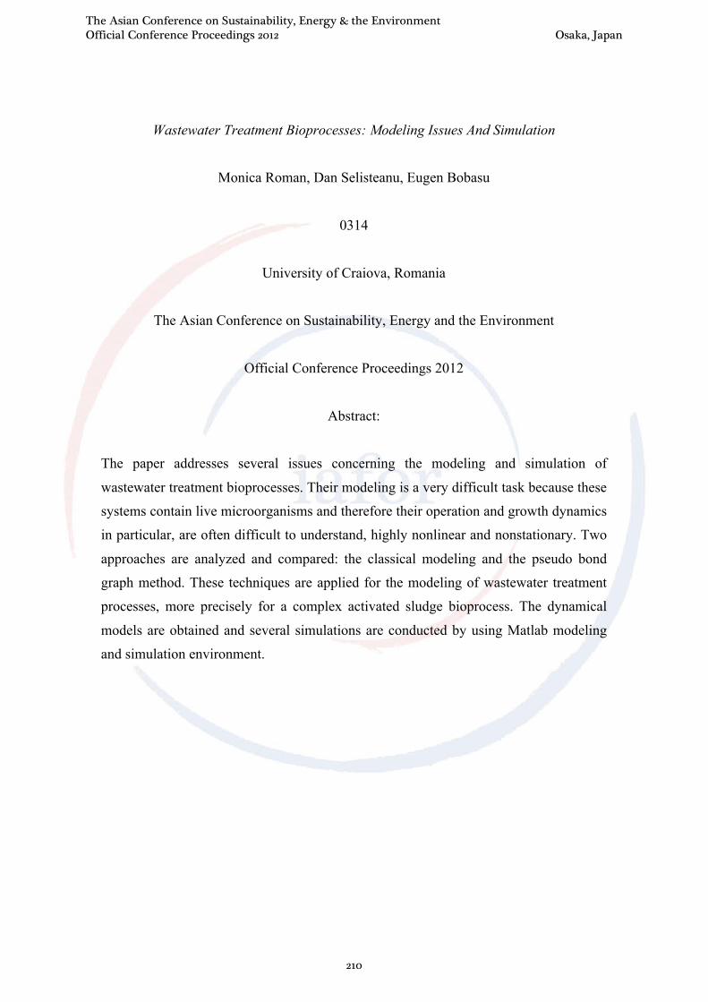
Wastewater Treatment Bioprocesses: Modeling Issues And Simulation

Monica Roman, Dan Selisteanu, Eugen Bobasu

0314

University of Craiova, Romania

The Asian Conference on Sustainability, Energy and the Environment

Official Conference Proceedings 2012

Abstract:

The paper addresses several issues concerning the modeling and simulation of

wastewater treatment bioprocesses. Their modeling is a very difficult task because these

systems contain live microorganisms and therefore their operation and growth dynamics

in particular, are often difficult to understand, highly nonlinear and nonstationary. Two

approaches are analyzed and compared: the classical modeling and the pseudo bond

graph method. These techniques are applied for the modeling of wastewater treatment

processes, more precisely for a complex activated sludge bioprocess. The dynamical

models are obtained and several simulations are conducted by using Matlab modeling

and simulation environment.

The Asian Conference on Sustainability, Energy & the Environment Official Conference Proceedings 2012 Osaka, Japan

210

1. Introduction

Human impact on the environment is beyond pollution, the term being more comprehensive than environmental deterioration. The environmental deterioration means the alteration of physical, chemical and structural components of the natural environment, reducing biological diversity and productivity of natural and anthropogenic ecosystems, ecological balance and impaired quality of life caused mainly by water pollution, air and soil pollution, overexploitation of natural resources, and by poor management and recovery [1]. Any substance (chemical, biological) solid, liquid, gaseous or vapor or any form of energy generated by human activities that alters the equilibrium of its constituents and bodies lives causing damaging property when introduced into the environment, represents a pollutant. Each main sector of polluted environment is not independent, but as it is known among the various compartments of the ecosphere has permanent transfers of matter and energy with other sectors. Despite active measures for waste disposal, the most important substances with direct effect on water pollution are chemicals (chlorides, pesticides, oil, gas, heavy metals, and organic substances) and biological factors (pathogens, parasites, etc.) [2], [3]. For accurate measures of pollution control and environmental remediation, environmental monitoring systems were implemented based on process control. These systems aim to optimize the industrial processes for better efficiency and lower pollutant emissions. Together with surveillance, forecasting, warning and intervention systems that take into account the evaluation of the dynamics of quality characteristics of environmental factors, these measures can offer reliable and improved results for environment preservation [4]. In the context of environmental protection, the implementation of biotechnological processes used for wastewater treatment becomes a necessity. Superior performance regarding the exploitation of such processes can only be obtained by applying modern techniques, both in terms of proper technologies and methods of modeling, identification and control. From a systemic point of view, biotechnological processes and the wastewater treatment ones in particular have a highly nonlinear character. The bioprocesses’ modeling is a very difficult task: these systems contain live microorganisms and therefore their operation and growth dynamics in particular, are often difficult to understand, highly nonlinear and nonstationary. The most common biological wastewater treatment is based on the so-called activated sludge process [5], [6]. The classical modeling method for bioprocesses can be found in several papers and industrial applications [7], [8], [9]. The modeling of wastewater treatment bioprocesses followed this classical line, and a lot of useful examples can be found ([6], [10], [11], [12], [13], etc.). However, due to the diversity of the bioprocesses, there are some problems concerning the development of a unified modeling approach [14]. Also, for control purposes it is necessary to obtain reduced-order models, with some structural properties (linear – nonlinear decoupling, stable – unstable subsystems, the decoupling of uncertain kinetics, etc.). Taking into account these problems, a viable alternative to the classical modeling can be the bond graph method [14]. Bond graph method was introduced by H.M. Paynter, and further developed in several works, such as [15], [16]. The bond graph approach is a powerful tool for modeling, analysis and design of different kind of systems, such as electrical, mechanical, hydraulic, thermal, chemical [17], [18], [19], etc. Among the advantages of bond graph approach we can mention: offers a unified approach for all types of systems; due to causality assignment it gives the possibility of localization of the state


211

variables and achieving the mathematical model in terms of state space equations in an easier way than using classical methods; provides information regarding the structural properties of the system; offers the possibility of building some complex models by using interconnected submodels. The structure of the paper is as follows. Section 2 presents some issues regarding the wastewater treatment plants, including the block scheme and functioning principle. Section 3 addresses the bond graph modeling of a complex bioprocess. Actually, a wastewater treatment bioprocess is considered, and the corresponding bond graph model is derived. More precisely, a multi-reactor activated sludge process is studied and bond graph model of the anoxic reactor is obtained. In Section 4 several simulations are performed by using the obtained dynamical model, and the time profiles of the components’ concentrations are provided. The simulations are conducted in Matlab programming environment (registered trademark of The MathWorks Inc., USA). Finally, Section 5 collects the conclusions.

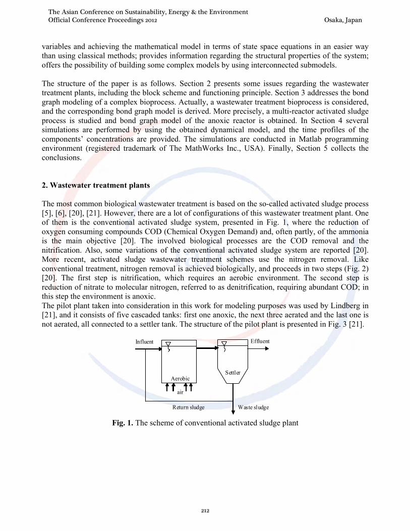
2. Wastewater treatment plants The most common biological wastewater treatment is based on the so-called activated sludge process [5], [6], [20], [21]. However, there are a lot of configurations of this wastewater treatment plant. One of them is the conventional activated sludge system, presented in Fig. 1, where the reduction of oxygen consuming compounds COD (Chemical Oxygen Demand) and, often partly, of the ammonia is the main objective [20]. The involved biological processes are the COD removal and the nitrification. Also, some variations of the conventional activated sludge system are reported [20]. More recent, activated sludge wastewater treatment schemes use the nitrogen removal. Like conventional treatment, nitrogen removal is achieved biologically, and proceeds in two steps (Fig. 2) [20]. The first step is nitrification, which requires an aerobic environment. The second step is reduction of nitrate to molecular nitrogen, referred to as denitrification, requiring abundant COD; in this step the environment is anoxic. The pilot plant taken into consideration in this work for modeling purposes was used by Lindberg in [21], and it consists of five cascaded tanks: first one anoxic, the next three aerated and the last one is not aerated, all connected to a settler tank. The structure of the pilot plant is presented in Fig. 3 [21].

Settler

Waste sludge Return sludge

air

Influent

Aerobic

Effluent

Fig. 1. The scheme of conventional activated sludge plant


212

Settler

Waste sludge

Return sludge

Influent

Anoxic

Effluent

air

Aerobic

Internal recirculation

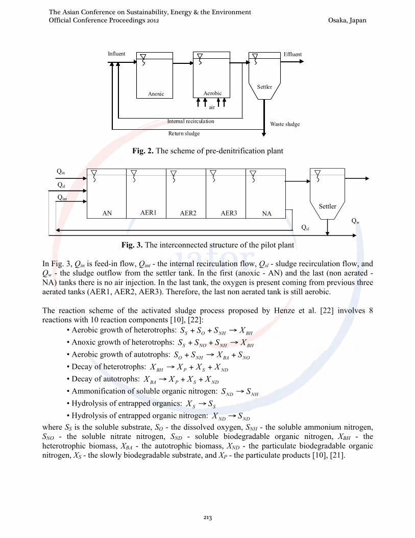
Fig. 2. The scheme of pre-denitrification plant

Settler AN

Qw

Qint

Qsl

AER1

Qin

AER2 AER3 NA

Qsl

Fig. 3. The interconnected structure of the pilot plant In Fig. 3, Qin is feed-in flow, Qint - the internal recirculation flow, Qsl - sludge recirculation flow, and Qw - the sludge outflow from the settler tank. In the first (anoxic - AN) and the last (non aerated - NA) tanks there is no air injection. In the last tank, the oxygen is present coming from previous three aerated tanks (AER1, AER2, AER3). Therefore, the last non aerated tank is still aerobic. The reaction scheme of the activated sludge process proposed by Henze et al. [22] involves 8 reactions with 10 reaction components [10], [22]:

• Aerobic growth of heterotrophs: BHNHOS XSSS →++ • Anoxic growth of heterotrophs: BHNHNOS XSSS →++ • Aerobic growth of autotrophs: NOBANHO SXSS +→+ • Decay of heterotrophs: NDSPBH XXXX ++→ • Decay of autotrophs: NDSPBA XXXX ++→ • Ammonification of soluble organic nitrogen: NHND SS → • Hydrolysis of entrapped organics: SS SX → • Hydrolysis of entrapped organic nitrogen: NDND SX →

where SS is the soluble substrate, SO - the dissolved oxygen, SNH - the soluble ammonium nitrogen, SNO - the soluble nitrate nitrogen, SND - soluble biodegradable organic nitrogen, XBH - the heterotrophic biomass, XBA - the autotrophic biomass, XND - the particulate biodegradable organic nitrogen, XS - the slowly biodegradable substrate, and XP - the particulate products [10], [21].


213

Due to the large number of the components associated to the biochemical process, and also because of the nonlinearity of the transformations within the process, for control purposes it is preferred a reduced order model developed using some simplifying assumptions [6]:

• the dissolved oxygen concentration in not taken into consideration; • the two fractions of organic matter SS, and XS are replaced by a single variable XCOD

considered to be measurable on-line; • also, the particulate products XP are removed in the reduced model; • only two of the four nitrogen fractions are considered in the reduced model, SNH and SNO (the

other two fractions SND and XND describe the formation of SNH, which is considered not to be so important for control purposes).

Taking into consideration these assumptions, the reduced model of the activated sludge bioprocess consists of 5 components, introducing a complete separation between the anoxic and the aerobic zones. One of the most difficult modeling procedures concerns the anoxic reactor. The anoxic tank is described by three reactions representing growth of heterotrophs, decay of heterotrophs and decay of autotrophs. The reaction scheme is as follows:

⎪⎪⎩

⎪⎪⎨

⎧

+⎯→⎯

+⎯→⎯

⎯→⎯++

ϕ

ϕ

ϕ

CODNHBA

CODNHBH

BHCODNHNO

XSX

XSX

XXSS

3

2

1

(1)

The reaction scheme (1) will be used in order to achieve the bond graph and the corresponding dynamical model. In the reaction scheme (1), 321 ,, ϕϕϕ are the reaction rates. 3. Modeling of wastewater treatment bioprocess The classical modeling of a wastewater treatment bioprocess follows the general modeling guidelines valid for a large class of bioprocesses. This approach is widely described in well known monographs such as [7], [10]. In this paper we propose a different technique, based on the bond graph methodology [15], [16], [23]. The result will be a bond graph model, from which a dynamical mathematical model (a set of nonlinear differential equations) will be obtained. This state-space model is equivalent with the model obtained via the classical approach. However, the bond graph model allows us to develop easily some estimation and control strategies, by using the inherent structural properties of a bond graph. Also, the modularity of the bond graph models gives the possibility to reuse the submodels in order to develop large models of interconnected reactors. Bond graph methodology provides a uniform manner to describe the dynamical behavior of all type of systems. In this paper we use an alternative of this method based on pseudo bonds, which is more suitable for chemical systems due to the physical meaning of the effort e and flow f variables involved. Two other types of variables are very important in describing dynamic systems and these are the generalized momentum p as time integral of effort and the generalized displacement q as time integral of flow [15], [16]. One of the advantages of this methodology is that models of various systems belonging to different engineering domains are represented using a small set of elements: inertial elements (I), capacitive elements (C), resistive elements (R), effort sources (Se) and flow sources (Sf), transformer elements (TF) and gyrator elements (GY), effort junctions (J0) and flow junctions (J1). In biochemical domain, the effort and flow variables have the signification of concentration and mass flow, respectively.


214

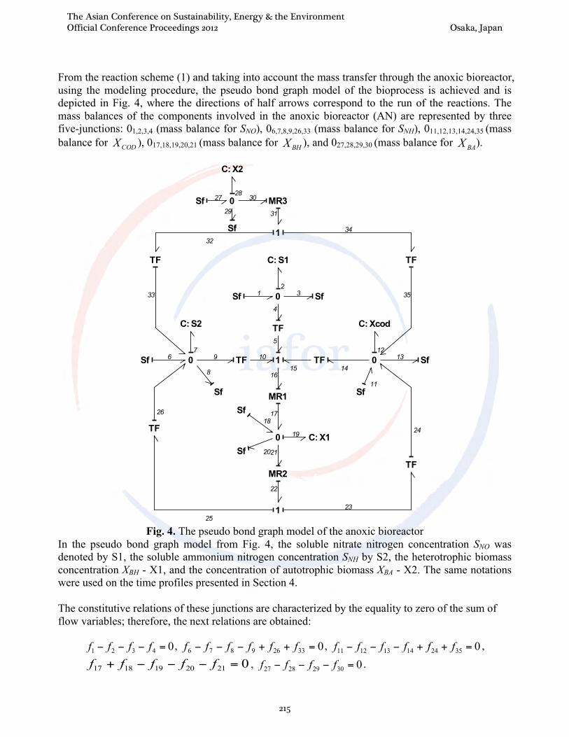
From the reaction scheme (1) and taking into account the mass transfer through the anoxic bioreactor, using the modeling procedure, the pseudo bond graph model of the bioprocess is achieved and is depicted in Fig. 4, where the directions of half arrows correspond to the run of the reactions. The mass balances of the components involved in the anoxic bioreactor (AN) are represented by three five-junctions: 01,2,3,4 (mass balance for SNO), 06,7,8,9,26,33 (mass balance for SNH), 011,12,13,14,24,35 (mass balance for CODX ), 017,18,19,20,21 (mass balance for BHX ), and 027,28,29,30 (mass balance for BAX ).

67

9 1012

141516

5

4

2

19

11

8

13

27

29

18

20

1 3

24

25

26

32

33 35

17

2830

31

34

21

22

23

0 1TF

C: S2

MR1

TF 0

C: S1

TF

0

C: Xcod

0 C: X1

1

1

C: X2

0

Sf

SfSf

Sf

Sf

Sf

Sf

Sf

Sf Sf

TF

TF

TF TF

MR3

MR2

Fig. 4. The pseudo bond graph model of the anoxic bioreactor

In the pseudo bond graph model from Fig. 4, the soluble nitrate nitrogen concentration SNO was denoted by S1, the soluble ammonium nitrogen concentration SNH by S2, the heterotrophic biomass concentration XBH - X1, and the concentration of autotrophic biomass XBA - X2. The same notations were used on the time profiles presented in Section 4. The constitutive relations of these junctions are characterized by the equality to zero of the sum of flow variables; therefore, the next relations are obtained:

04321 =−−− ffff , 033269876 =++−−− ffffff , 0352414131211 =++−−− ffffff , 02120191817 =−−−+ fffff , 030292827 =−−− ffff .


215

Thus, the accumulations of components NOS , NHS , CODX , BHX , and BAX inside the anoxic bioreactor are represented by bonds 2, 7, 12, 19, 28 are modeled using capacitive elements C. The constitutive equations of these elements are as follows:

NOS : ( )dtfffC

qC

et∫ −−== 431

22

22

11 , (2)

NHS : ( )dtfffffC

qC

et∫ ++−−== 3326986

77

77

11 , (3)

CODX : ( )dtfffffC

qC

et∫ ++−−== 3524141311

1212

1212

11 , (4)

BHX : ( )dtffffC

qC

et∫ −−+== 21201817

1919

1919

11 , (5)

BAX : ( )dtfffC

qC

et∫ −−== 302927

2828

2828

11 , (6)

where 2e , 7e , 12e , 19e and 28e are the concentrations of components NOS , NHS , CODX , BHX , and BAX (g/m3). The parameters corresponding to capacitive elements are equal to the anoxic bioreactor volume: 128191272 VCCCCC ===== , with 1V (m3) - the volume of the anoxic reactor. Mass flows of the components entering the bioreactor are modeled using source flow elements Sf1, Sf6, Sf11, Sf18, and Sf27. The output flows of the components are also modeled using Sf elements represented by bonds 3, 8, 13, 20, 29. The constitutive equations of these elements are: 333 eSff = ,

888 eSff = , 131313 eSff = , 202020 eSff = , 292929 eSff = , where 3Sf , 8Sf , 13Sf , 20Sf , 29Sf are the parameters of Sf-elements and they are equal to the output flow of the anoxic bioreactor ZQ ⋅ (m3/h), slin QQQQ ++= int , and Z is the concentration of the corresponding component. The

transformer elements TF were introduced to model the yield coefficients 7,1, =iki , and for the modeling of the reaction kinetics we used three modulated two-port R-elements: MR1, MR2, and MR3. From the constitutive relations of 1-junction elements 15,10,15,16, 122,23,25, and 131,32,34 we obtain:

1615105 ffff === , 252322 fff == , 343231 fff == , where the constitutive relations of MR elements imply that 1116 Vf ϕ= , 1222 Vf ϕ= , 1331 Vf ϕ= , with 1ϕ , 2ϕ , 3ϕ being the reaction rates;

191 eHµ=ϕ , 192 ebH=ϕ , 283 ebA=ϕ , Hµ - the specific growth rate of heterotrophs, bH, bA – the decay rate of heterotrophs and autotrophs. The signification of bond graph elements is as follows: 2e is the soluble nitrate nitrogen concentration SNO (g/m3), 7e - the soluble ammonium nitrogen concentration SNH (g/m3), 12e - the organic matter concentration XCOD (g/m3), 19e is the heterotrophic biomass concentration XBH (g/m3

),

28e is the concentration of autotrophic biomass, XBA (g/m3); the input flows f1, f6, f11, f18, and f27 are equal to the corresponding QinZin + QintZint + QslZsl (g/h), where Z represents the concentration of each component. Using these notations, from (2)-(6) we will obtain the mass balance equations of the bioprocess from the anoxic tank:


216

BHCODHNOslinslNOslNOinNOin

NO XXrkSV

QQQV

SQSQSQS 1

1

int

1

intint −++

−++

= (7)

BAABHH

BHCODHNHslinslNHslNHinNHin

NH

XbkXbk

XXrkSV

QQQV

SQSQSQS

43

21

int

1

intint

++

+−++

−++

= (8)

BAABHH

BHCODHCODslinslCODslCODinCODin

COD

XbXb

XXrkXV

QQQV

XQXQXQX

++

+−++

−++

= 51

int

1

intint (9)

BHH

BHCODHBHslinslBHslBHinBHin

BH

Xb

XXrXV

QQQV

XQXQXQX

−

−+++

−++

=1

int

1

intint (10)

BAABAslinslBAslBAinBAin

BA XbXV

QQQV

XQXQXQX −

++−

++=

1

int

1

intint (11)

where the production coefficients are: H

H

YYk86,21

1−

= , XBikkk === 432 , HY

k 15 = , with HY - the

heterotrophic yield and XBi - mass N/mass COD in biomass. The specific growth rate of heterotrophs is modeled using a double Monod law:

⎟⎟⎠

⎞⎜⎜⎝

⎛

+⎟⎟⎠

⎞⎜⎜⎝

⎛

+=

CODSNONO

NOHH XKSK

Sr 1

µ

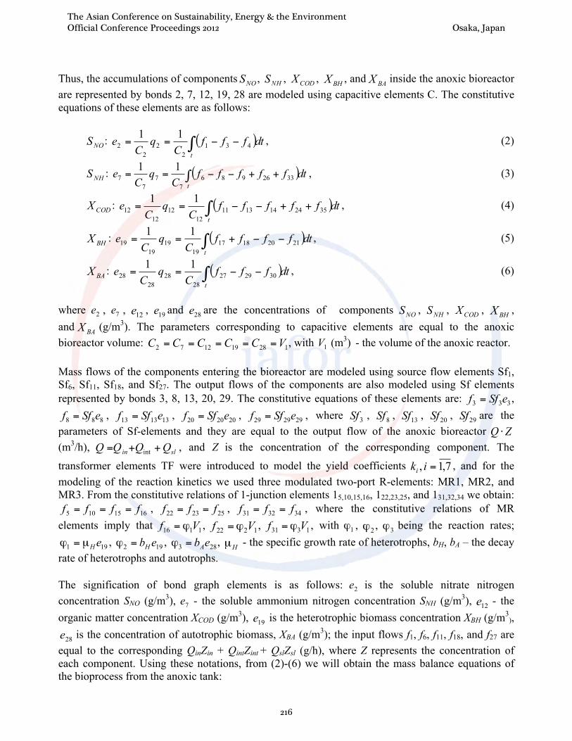
where NOK is the nitrate half-saturation coefficient for denitrifying heterotrophs, and SK is the half-saturation coefficient for heterotrophs. Thus, the model of the anoxic reactor is represented by relations (7)-(11). However, to obtain the full model of interconnected reactors, it is necessary to design the bond graph models of the aerobic reactors and of the non aerated reactor. Then the full dynamical model can be obtained by combining the corresponding submodels. 4. Simulation results The behavior of the obtained bioprocess model was tested using numerical simulations, by using the Matlab programming environment (registered trademark of the MathWorks Inc., USA). The wastewater treatment bioprocess has been simulated for process parameters presented in Table 1 [6]. The values of influent concentrations are given in Table 2, and the initial conditions of state variables, in Table 3 [6].


217

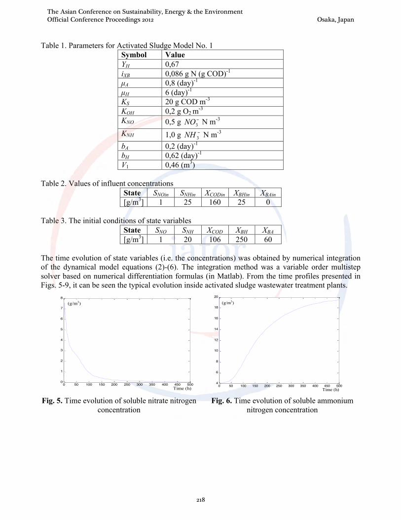
Table 1. Parameters for Activated Sludge Model No. 1 Symbol Value YH 0,67 iXB 0,086 g N (g COD)-1 µA 0,8 (day)-1 µH 6 (day)-1

KS 20 g COD m-3

KOH 0,2 g O2 m-3

KNO 0,5 g −3NO N m-3

KNH 1,0 g −3NH N m-3

bA 0,2 (day)-1 bH 0,62 (day)-1 V1 0,46 (m3)

Table 2. Values of influent concentrations

State SNOin SNHin XCODin XBHin XBAin [g/m3] 1 25 160 25 0

Table 3. The initial conditions of state variables

State SNO SNH XCOD XBH XBA [g/m3] 1 20 106 250 60

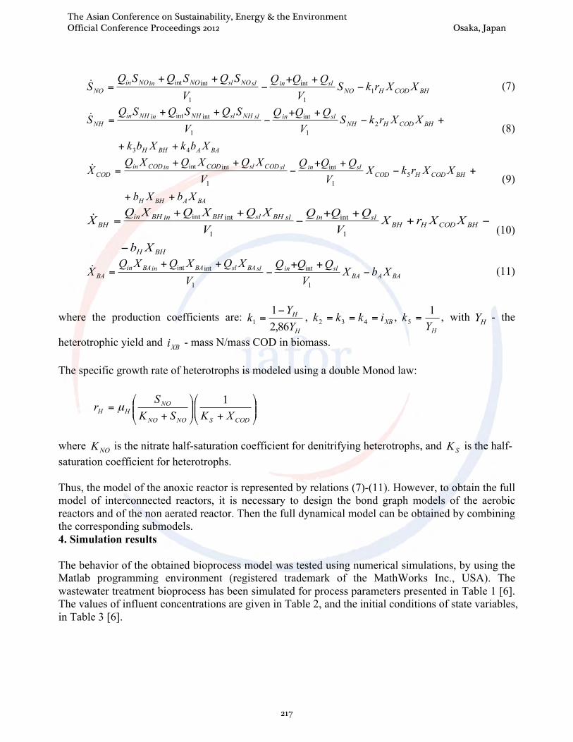
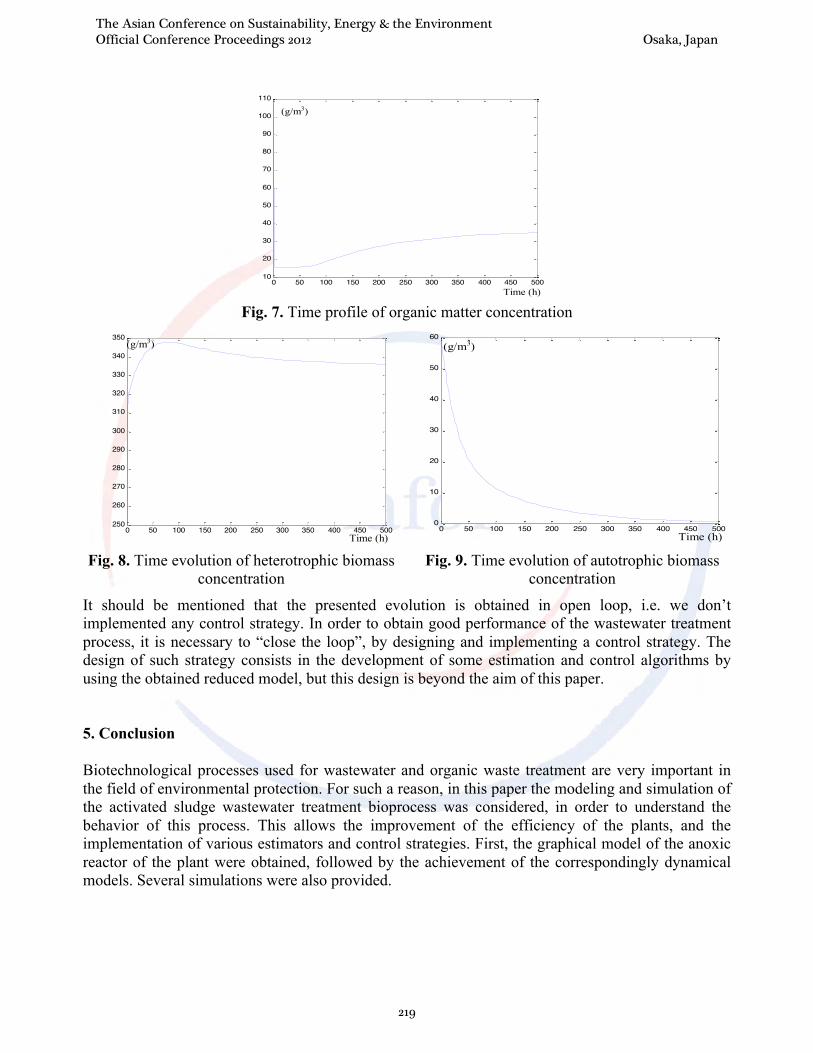
The time evolution of state variables (i.e. the concentrations) was obtained by numerical integration of the dynamical model equations (2)-(6). The integration method was a variable order multistep solver based on numerical differentiation formulas (in Matlab). From the time profiles presented in Figs. 5-9, it can be seen the typical evolution inside activated sludge wastewater treatment plants.

0 50 100 150 200 250 300 350 400 450 5000

1

2

3

4

5

6

7

8

Time (h)

(g/m3)

0 50 100 150 200 250 300 350 400 450 500

4

6

8

10

12

14

16

18

20

Time (h)

(g/m3)

Fig. 5. Time evolution of soluble nitrate nitrogen

concentration Fig. 6. Time evolution of soluble ammonium

nitrogen concentration


218

0 50 100 150 200 250 300 350 400 450 50010

20

30

40

50

60

70

80

90

100

110

Time (h)

(g/m3)

Fig. 7. Time profile of organic matter concentration

0 50 100 150 200 250 300 350 400 450 500250

260

270

280

290

300

310

320

330

340

350

Time (h)

(g/m3)

0 50 100 150 200 250 300 350 400 450 500

0

10

20

30

40

50

60

Time (h)

(g/m3)

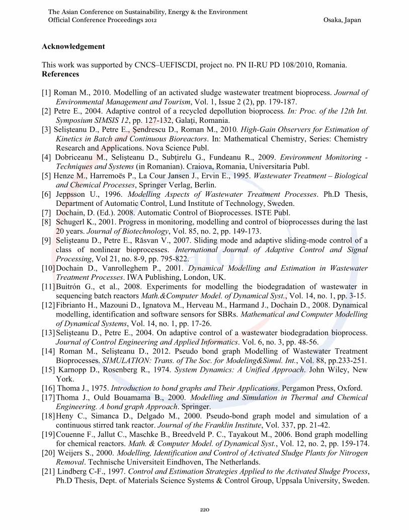
Fig. 8. Time evolution of heterotrophic biomass

concentration Fig. 9. Time evolution of autotrophic biomass

concentration

It should be mentioned that the presented evolution is obtained in open loop, i.e. we don’t implemented any control strategy. In order to obtain good performance of the wastewater treatment process, it is necessary to “close the loop”, by designing and implementing a control strategy. The design of such strategy consists in the development of some estimation and control algorithms by using the obtained reduced model, but this design is beyond the aim of this paper. 5. Conclusion

Biotechnological processes used for wastewater and organic waste treatment are very important in the field of environmental protection. For such a reason, in this paper the modeling and simulation of the activated sludge wastewater treatment bioprocess was considered, in order to understand the behavior of this process. This allows the improvement of the efficiency of the plants, and the implementation of various estimators and control strategies. First, the graphical model of the anoxic reactor of the plant were obtained, followed by the achievement of the correspondingly dynamical models. Several simulations were also provided.


219

Acknowledgement This work was supported by CNCS–UEFISCDI, project no. PN II-RU PD 108/2010, Romania. References [1] Roman M., 2010. Modelling of an activated sludge wastewater treatment bioprocess. Journal of

Environmental Management and Tourism, Vol. 1, Issue 2 (2), pp. 179-187. [2] Petre E., 2004. Adaptive control of a recycled depollution bioprocess. In: Proc. of the 12th Int.

Symposium SIMSIS 12, pp. 127-132, Galaţi, Romania. [3] Selişteanu D., Petre E., Şendrescu D., Roman M., 2010. High-Gain Observers for Estimation of

Kinetics in Batch and Continuous Bioreactors. In: Mathematical Chemistry, Series: Chemistry Research and Applications. Nova Science Publ.

[4] Dobriceanu M., Selişteanu D., Subţirelu G., Fundeanu R., 2009. Environment Monitoring - Techniques and Systems (in Romanian). Craiova, Romania, Universitaria Publ.

[5] Henze M., Harremoës P., La Cour Jansen J., Ervin E., 1995. Wastewater Treatment – Biological and Chemical Processes, Springer Verlag, Berlin.

[6] Jeppsson U., 1996. Modelling Aspects of Wastewater Treatment Processes. Ph.D Thesis, Department of Automatic Control, Lund Institute of Technology, Sweden.

[7] Dochain, D. (Ed.). 2008. Automatic Control of Bioprocesses. ISTE Publ. [8] Schugerl K., 2001. Progress in monitoring, modelling and control of bioprocesses during the last

20 years. Journal of Biotechnology, Vol. 85, no. 2, pp. 149-173. [9] Selişteanu D., Petre E., Răsvan V., 2007. Sliding mode and adaptive sliding-mode control of a

class of nonlinear bioprocesses. International Journal of Adaptive Control and Signal Processing, Vol 21, no. 8-9, pp. 795-822.

[10] Dochain D., Vanrolleghem P., 2001. Dynamical Modelling and Estimation in Wastewater Treatment Processes. IWA Publishing, London, UK.

[11] Buitrón G., et al., 2008. Experiments for modelling the biodegradation of wastewater in sequencing batch reactors Math.&Computer Model. of Dynamical Syst., Vol. 14, no. 1, pp. 3-15.

[12] Fibrianto H., Mazouni D., Ignatova M., Herveau M., Harmand J., Dochain D., 2008. Dynamical modelling, identification and software sensors for SBRs. Mathematical and Computer Modelling of Dynamical Systems, Vol. 14, no. 1, pp. 17-26.

[13] Selişteanu D., Petre E., 2004. On adaptive control of a wastewater biodegradation bioprocess. Journal of Control Engineering and Applied Informatics. Vol. 6, no. 3, pp. 48-56.

[14] Roman M., Selişteanu D., 2012. Pseudo bond graph Modelling of Wastewater Treatment Bioprocesses. SIMULATION: Trans. of The Soc. for Modeling&Simul. Int., Vol. 88, pp.233-251.

[15] Karnopp D., Rosenberg R., 1974. System Dynamics: A Unified Approach. John Wiley, New York.

[16] Thoma J., 1975. Introduction to bond graphs and Their Applications. Pergamon Press, Oxford. [17] Thoma J., Ould Bouamama B., 2000. Modelling and Simulation in Thermal and Chemical

Engineering. A bond graph Approach. Springer. [18] Heny C., Simanca D., Delgado M., 2000. Pseudo-bond graph model and simulation of a

continuous stirred tank reactor. Journal of the Franklin Institute, Vol. 337, pp. 21-42. [19] Couenne F., Jallut C., Maschke B., Breedveld P. C., Tayakout M., 2006. Bond graph modelling

for chemical reactors. Math. & Computer Model. of Dynamical Syst., Vol. 12, no. 2, pp. 159-174. [20] Weijers S., 2000. Modelling, Identification and Control of Activated Sludge Plants for Nitrogen

Removal. Technische Universiteit Eindhoven, The Netherlands. [21] Lindberg C-F., 1997. Control and Estimation Strategies Applied to the Activated Sludge Process,

Ph.D Thesis, Dept. of Materials Science Systems & Control Group, Uppsala University, Sweden.


220

[22] Henze M., Grady Jr. C.P.L., Gujer W., Marais G.v.R., Matsuo T., 1987. Activated Sludge Model No. 1 – IAWQ Scientific and Technical Report No. 1, IAWQ, London, Great Britain.

[23] Dauphin-Tanguy G. (Ed.), 2000. Les bond graphs. Hermes Sci., Paris.


221

Documents

Wastewater Treatment Bioprocesses: Modeling … Treatment Bioprocesses: Modeling Issues And Simulation ... are conducted by using Matlab modeling and simulation ... is a powerful tool