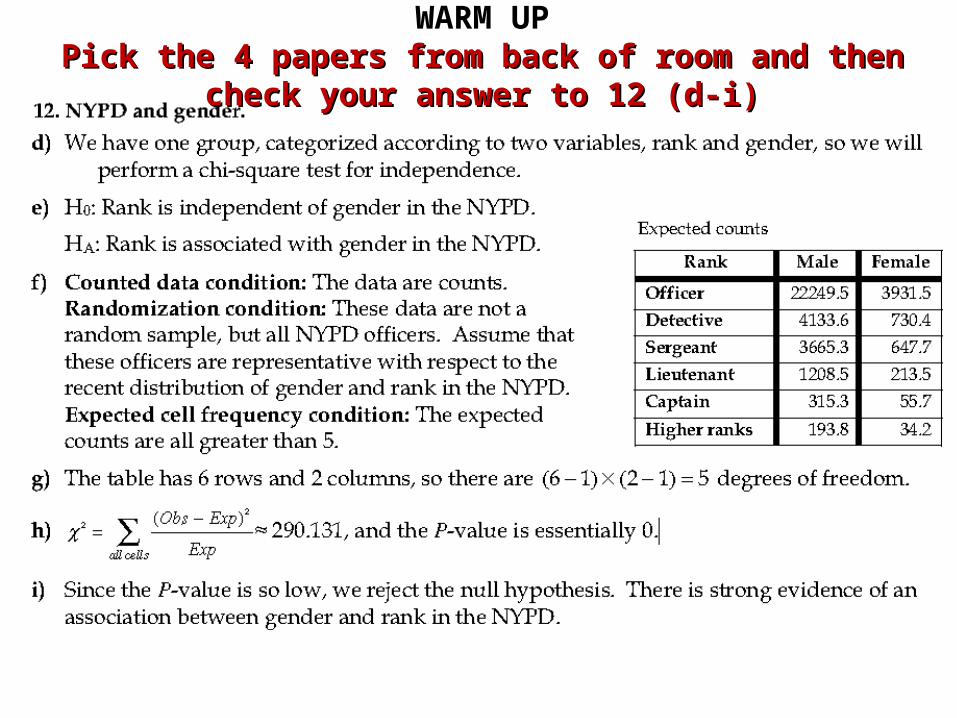
WARM UPPick the 4 papers from back of room and then check your Pick the 4 papers from back of room and then check your

answer to 12 (d-i)answer to 12 (d-i)

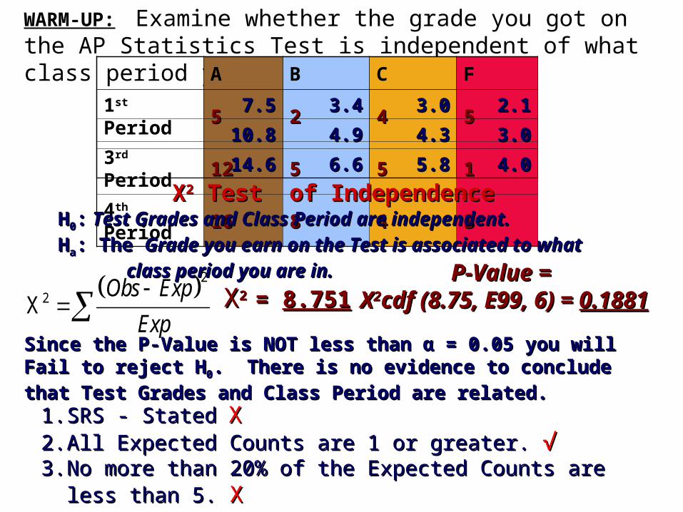
WARM-UP: Examine whether the grade you got on the AP Statistics Test is independent of what class period you are in.

A B C F

1st Period 55 22 44 55

3rd Period 1212 55 55 11

4th Period 1616 88 44 33

22XObs Exp

Exp

XX22 Test of Independence Test of Independence

P-Value = P-Value = XX22cdf cdf (8.75, E99, 6) = (8.75, E99, 6) = 0.18810.1881

HH00:: Test Grades and Class Period are independent. Test Grades and Class Period are independent.

HHaa: The : The Grade you earn on the Test is associated to what Grade you earn on the Test is associated to what

class period you are in.class period you are in.

XX2 2 = = 8.7518.751

7.57.5 3.43.4 3.03.0 2.12.1

10.810.8 4.94.9 4.34.3 3.03.0

14.614.6 6.66.6 5.85.8 4.04.0

Since the P-Value is NOT less than Since the P-Value is NOT less than αα = 0.05 you will Fail to reject H = 0.05 you will Fail to reject H00. .

There is no evidence to conclude that Test Grades and Class Period There is no evidence to conclude that Test Grades and Class Period are related.are related.

1.1. SRS - StatedSRS - Stated XX2.2. All Expected Counts are 1 or greater.All Expected Counts are 1 or greater. √√ 3.3. No more than 20% of the Expected Counts are less than 5. No more than 20% of the Expected Counts are less than 5. XX

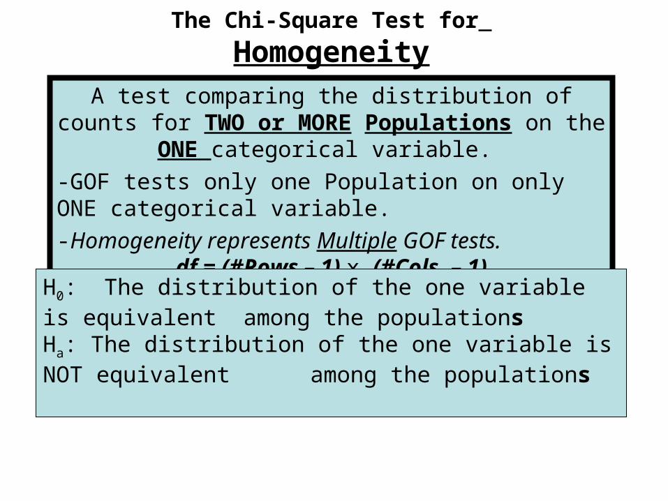
The Chi-Square Test for

Homogeneity

A test comparing the distribution of counts for TWO or MORE Populations on the ONE categorical variable.

-GOF tests only one Population on only ONE categorical variable.

-Homogeneity represents Multiple GOF tests. df = (#Rows – 1) x (#Cols. – 1)

H0: The distribution of the one variable is equivalent among the populationsHa: The distribution of the one variable is NOT equivalent

among the populations

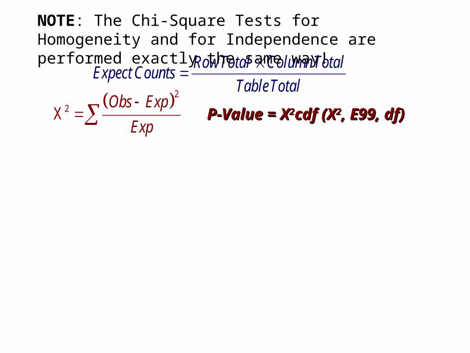
RowTotal ColumnTotalExpect Counts

TableTotal

P-Value = P-Value = XX22cdf cdf (X(X22, E99, df), E99, df) 22XObs Exp

Exp

NOTE: The Chi-Square Tests for Homogeneity and for Independence are performed exactly the same way!

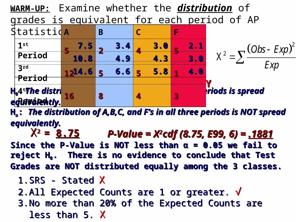
WARM-UP: Examine whether the distribution of grades is equivalent for each period of AP Statistics.

22XObs Exp

Exp

XX22 Test of HOMOGENEITY Test of HOMOGENEITY

P-Value = P-Value = XX22cdf cdf (8.75, E99, 6) = (8.75, E99, 6) = .1881.1881

HH00:: The distribution of A,B,C, and F’s in all three periods is spread The distribution of A,B,C, and F’s in all three periods is spread

equivalently. equivalently. HHaa: : The distribution of A,B,C, and F’s in all three periods is NOT spread The distribution of A,B,C, and F’s in all three periods is NOT spread

equivalently. equivalently. XX2 2 = = 8.758.75

Since the P-Value is NOT less than Since the P-Value is NOT less than αα = 0.05 we fail to reject H = 0.05 we fail to reject H00. There . There

is no evidence to conclude that Test Grades are NOT distributed is no evidence to conclude that Test Grades are NOT distributed equally among the 3 classes.equally among the 3 classes.

1.1. SRS - StatedSRS - Stated XX2.2. All Expected Counts are 1 or greater.All Expected Counts are 1 or greater. √√ 3.3. No more than 20% of the Expected Counts are less than 5. No more than 20% of the Expected Counts are less than 5. XX

A B C F

1st Period 55 22 44 55

3rd Period 1212 55 55 11

4th Period 1616 88 44 33

7.57.5 3.43.4 3.03.0 2.12.1

10.810.8 4.94.9 4.34.3 3.03.0

14.614.6 6.66.6 5.85.8 4.04.0

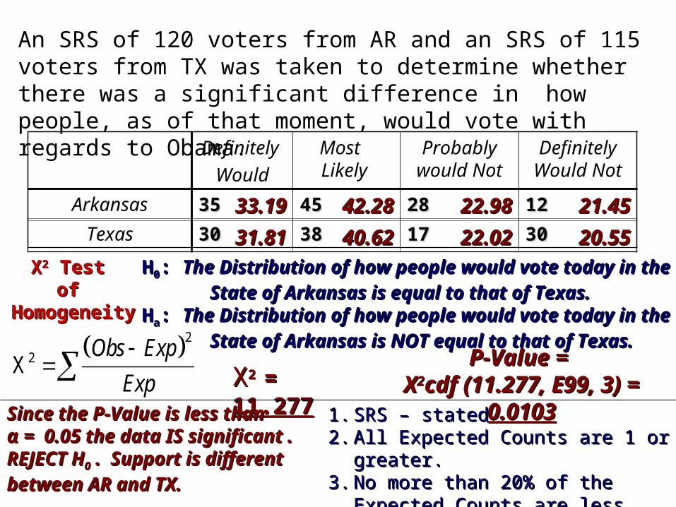
An SRS of 120 voters from AR and an SRS of 115 voters from TX was taken to determine whether there was a significant difference in how people, as of that moment, would vote with regards to Obama.

Definitely

Would

Mostly Likely

Probably would Not

Definitely Would Not

Arkansas 3535 4545 2828 1212

Texas 3030 3838 1717 3030

XX2 2 = = 11.27711.277 22XObs Exp

Exp

XX22 Test Test of of

Homogeneity Homogeneity

P-Value = P-Value = XX22cdf cdf (11.277, E99, 3) = (11.277, E99, 3) =

0.01030.0103

HH00: : The Distribution of how people would vote today in the The Distribution of how people would vote today in the

State of Arkansas is equal to that of Texas.State of Arkansas is equal to that of Texas.HHaa: : The Distribution of how people would vote today in the The Distribution of how people would vote today in the

State of Arkansas is NOT equal to that of Texas.State of Arkansas is NOT equal to that of Texas.

33.1933.19 42.2842.28 22.9822.98 21.4521.45

31.8131.81 40.6240.62 22.0222.02 20.5520.55

Since the P-Value is less than Since the P-Value is less than αα = 0.05 the data IS significant . = 0.05 the data IS significant . REJECT HREJECT H00 . Support is different . Support is different

between AR and TX.between AR and TX.

1.1. SRS – statedSRS – stated2.2. All Expected Counts are 1 or greater.All Expected Counts are 1 or greater.3.3. No more than 20% of the Expected No more than 20% of the Expected

Counts are less than 5.Counts are less than 5.

#18

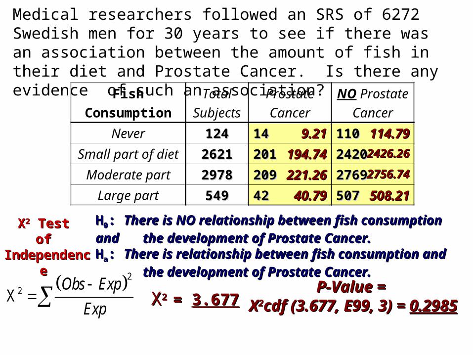
Medical researchers followed an SRS of 6272 Swedish men for 30 years to see if there was an association between the amount of fish in their diet and Prostate Cancer. Is there any evidence of such an association?

Fish

Consumption

Total

Subjects

Prostate

Cancer

Never 124124 1414

Small part of diet 26212621 201201

Moderate part 29782978 209209

Large part 549549 4242

NO Prostate

Cancer

1414 110110

201201 24202420

209209 27692769

4242 507507

9.219.21 114.79114.79

194.74194.74 2426.262426.26

221.26221.26 2756.742756.74

40.7940.79 508.21508.21

22XObs Exp

Exp

XX22 Test Test of of

Independence Independence

P-Value = P-Value = XX22cdf cdf (3.677, E99, 3) = (3.677, E99, 3) =

0.29850.2985

HH00: : There is NO relationship between fish consumption and There is NO relationship between fish consumption and

the development of Prostate Cancer.the development of Prostate Cancer.HHaa: : There is relationship between fish consumption and There is relationship between fish consumption and

the development of Prostate Cancer.the development of Prostate Cancer.

XX2 2 = = 3.6773.677

Fish

Consumption

Total

Subjects

Prostate

Cancer

Never 124124 1414

Small part of diet 26212621 201201

Moderate part 29782978 209209

Large part 549549 4242

NO Prostate

Cancer

1414 110110

201201 24202420

209209 27692769

4242 507507

9.219.21 114.79114.79

194.74194.74 2426.262426.26

221.26221.26 2756.742756.74

40.7940.79 508.21508.21

22XObs Exp

Exp

XX22 Test Test of of

Independence Independence

P-Value = P-Value = XX22cdf cdf (3.677, E99, 3) = (3.677, E99, 3) =

0.29850.2985

HH00: : There is NO relationship between fish consumption and There is NO relationship between fish consumption and

the development of Prostate Cancer.the development of Prostate Cancer.HHaa: : There is relationship between fish consumption and There is relationship between fish consumption and

the development of Prostate Cancer.the development of Prostate Cancer.

XX2 2 = = 3.6773.677

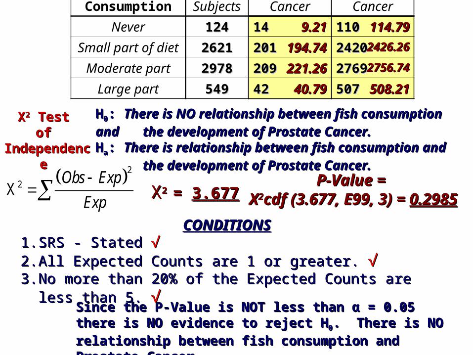
Since the P-Value is NOT less than Since the P-Value is NOT less than αα = 0.05 there is NO = 0.05 there is NO evidence to reject Hevidence to reject H00. There is NO relationship between . There is NO relationship between

fish consumption and Prostate Cancer.fish consumption and Prostate Cancer.

CONDITIONSCONDITIONS1.1. SRS - Stated SRS - Stated √√ 2.2. All Expected Counts are 1 or greater.All Expected Counts are 1 or greater. √√3.3. No more than 20% of the Expected Counts are less than 5. No more than 20% of the Expected Counts are less than 5. √√

WARM – UP

Does ones regional location have an affect on their Political affiliation? To begin to investigate this situation data from 177 voters was analyzed.

Democrat Republican

West 39 27

Northeast 35 15

Southeast 17 44

Political Affiliation

Lo

cati

on

a.)a.) Find the Proportion of Find the Proportion of Democrats in each region.Democrats in each region.

b.)b.) Make a Bar Chart for the Prop. Make a Bar Chart for the Prop.

c.)c.) Find the Expected Values for Find the Expected Values for each cell.each cell.

0.5910.591

0.7000.700

0.2790.279

% o

f D

em.

0

50

100

N NW SERegional Location

32.0732.07

24.2924.29

29.6429.64

33.9333.93

25.7125.71

31.3631.36

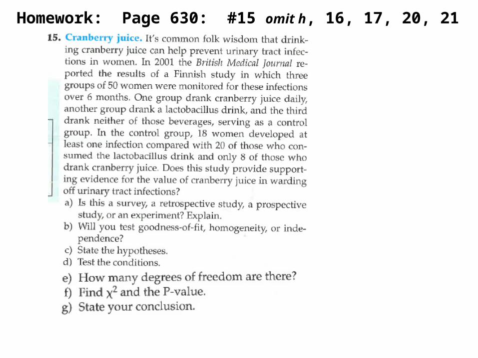
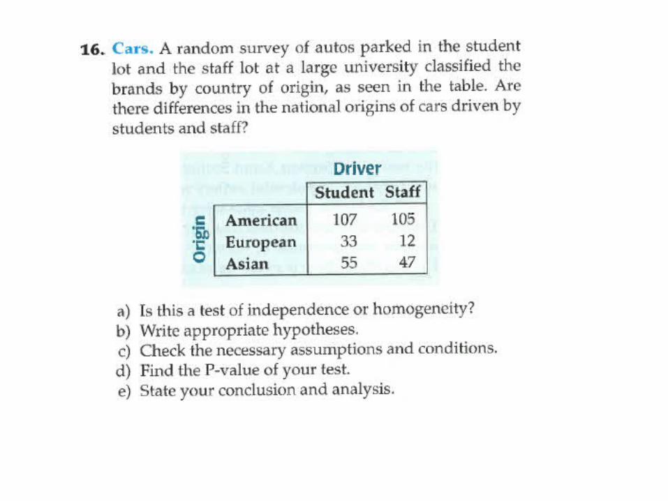
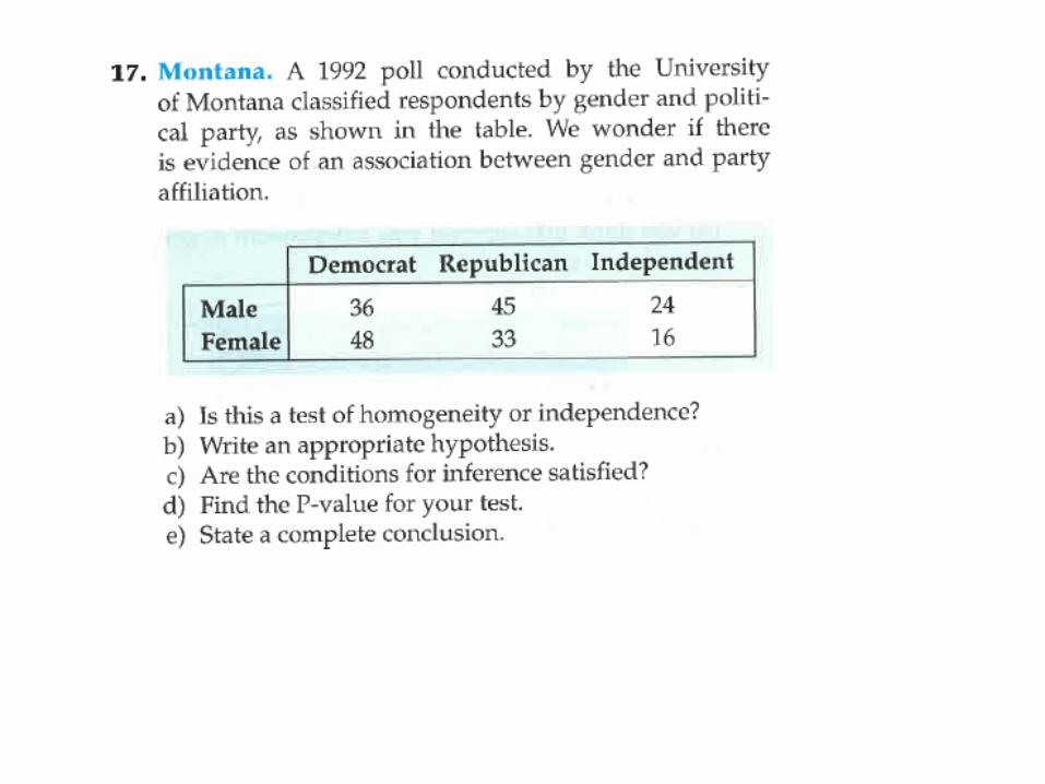
Homework: Page 630: #15 omit h, 16, 17, 20, 21

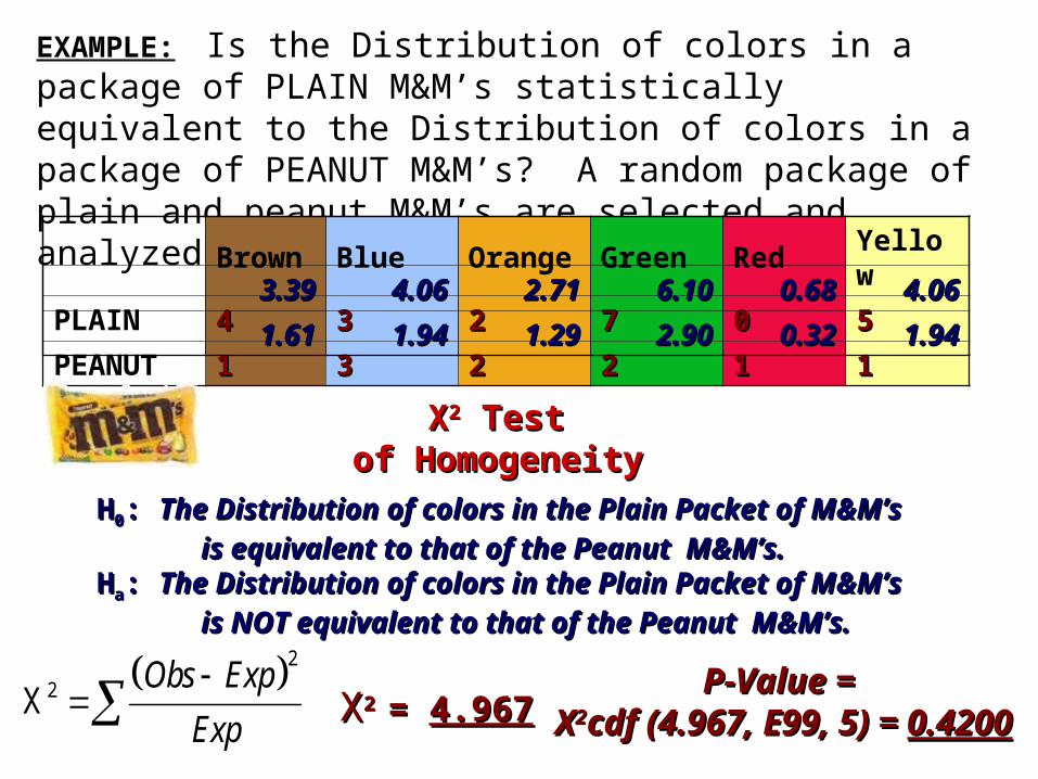
EXAMPLE: Is the Distribution of colors in a package of PLAIN M&M’s statistically equivalent to the Distribution of colors in a package of PEANUT M&M’s? A random package of plain and peanut M&M’s are selected and analyzed.

Brown Blue Orange Green Red Yellow

PLAIN 44 33 22 77 00 55

PEANUT 11 33 22 22 11 11

22XObs Exp

Exp

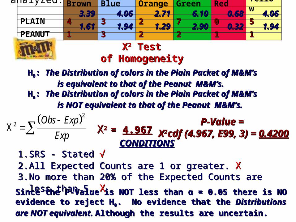
XX22 Test Test of Homogeneityof Homogeneity

P-Value = P-Value = XX22cdf cdf (4.967, E99, 5) = (4.967, E99, 5) =

0.42000.4200

HH00: : The Distribution of colors in the Plain Packet of M&M’s The Distribution of colors in the Plain Packet of M&M’s

is equivalent to that of the Peanut M&M’s.is equivalent to that of the Peanut M&M’s.HHaa: : The Distribution of colors in the Plain Packet of M&M’s The Distribution of colors in the Plain Packet of M&M’s

is NOT equivalent to that of the Peanut M&M’s.is NOT equivalent to that of the Peanut M&M’s.

XX2 2 = = 4.9674.967

3.393.39 4.064.06 2.712.71 6.106.10 0.680.68 4.064.06

1.611.61 1.941.94 1.291.29 2.902.90 0.320.32 1.941.94

Brown Blue Orange Green Red Yellow

PLAIN 44 33 22 77 00 55

PEANUT 11 33 22 22 11 11

22XObs Exp

Exp

XX22 Test Test of Homogeneityof Homogeneity

P-Value = P-Value = XX22cdf cdf (4.967, E99, 3) = (4.967, E99, 3) =

0.42000.4200

HH00: : The Distribution of colors in the Plain Packet of M&M’s The Distribution of colors in the Plain Packet of M&M’s

is equivalent to that of the Peanut M&M’s.is equivalent to that of the Peanut M&M’s.HHaa: : The Distribution of colors in the Plain Packet of M&M’s The Distribution of colors in the Plain Packet of M&M’s

is NOT equivalent to that of the Peanut M&M’s.is NOT equivalent to that of the Peanut M&M’s.

XX2 2 = = 4.9674.967

Since the P-Value is NOT less than Since the P-Value is NOT less than αα = 0.05 there is NO evidence to = 0.05 there is NO evidence to reject Hreject H00. No evidence that the . No evidence that the Distributions are NOT equivalent. Distributions are NOT equivalent.

Although the results are uncertain.Although the results are uncertain.

CONDITIONSCONDITIONS1.1. SRS - Stated SRS - Stated √√ 2.2. All Expected Counts are 1 or greater.All Expected Counts are 1 or greater. XX3.3. No more than 20% of the Expected Counts are less than 5. No more than 20% of the Expected Counts are less than 5. XX

3.393.39 4.064.06 2.712.71 6.106.10 0.680.68 4.064.06

1.611.61 1.941.94 1.291.29 2.902.90 0.320.32 1.941.94