WANs and Long Distance Connectivity

Chapters 12-13

Introduction

• Previous technologies covered "short" distances – Can extend over short distances somewhat with bridges, hubs,

repeaters, etc. but still limited

– We need to cover longer distances - e.g. Anchorage to Seattle

• Will call this technology WAN - Wide Area Network • Two categories:

– Long distance between networks

– "Local loop" - the copper between the Telco’s CO and the subscriber (e.g., home)

Digital Telephony

• Analog used in olden days throughout the telco– Problem of amplifying noise, distortion

• Telco uses digital technology today– Thanks in large part to fiber optics– High initial cost in conversion– Benefit of packet switched technology, reduced problems with

noise

• Voice digitized and sent digitally– Recall PCM : Pulse Code Modulation– 8000 samples per second (twice the bandwidth), each sample

value 0-255– Requires 64Kbps throughput to transmit digitized voice

Synchronous Communications

• Telephone Network uses synchronous communications– Converting back to audio requires data be available

"on time" – Digital telephony systems use clocking for

synchronous data delivery – Samples not delayed as traffic increases – Telephone system carefully designed so the rate of

data on receiver is the same as the rate that it entered• Consider understanding a voice call if these rates were

different!

Digital Circuits and Computer Data

• So, digital telephony can handle synchronous data delivery – Can we use that for data delivery? – Ethernet frame != 8-bit PCM synchronous – Need to convert formats...

• To use digital telephony for data delivery: – Lease point-to-point digital circuit between sites – Convert between local and PCM formats at each end

• Use a Data Service Unit/Channel Service Unit (DSU/CSU) at each end – CSU - manages control functions – DSU - converts data – Telco analogy to a modem

Using a CSU/DSU

Many different CSU/DSU’s out there, supporting different protocols

Telephone Standards• Most common standard is the T-series• European standards start with E• The T standard doesn’t specify the physical media

– Could use satellite, copper, fiber, etc.– Specifies data rates, multiplexing is common

Name Bit Rate Voice Circuits Location

ISDN 0.064Mbps 1

T1 1.544Mbps 24 NA

T2 6.312Mbps 96 NA

T3 44.736Mbps 672 NA

E1 2.048Mbps 30 Europe

E2 8.448Mbps 120 Europe

E3 34.368Mbps 480 Europe

28 T1’s

Terminology and Variations

• T standard technically different than DS standard, although the terms are used interchangeably in practice

• DS = Digital Signal Level Standards– DS1 = digital service that can multiplex 24 calls into a single

circuit– i.e. T1 speeds– Most popular are T1 and T3, or DS1 and DS3

• What if you don’t want an entire T1?– Expensive, generally too much for individuals– Fractional T1 is an option

• Lease capacity in chunks of 64K, e.g. 128Kbps, or 56Kbps too• Phone company uses TDM to subdivide the T1 circuit

Intermediate Capacity

• Price does not go up linearly with speed – $$ for T3 < $$ for 28 * T1

...however, if all you need is 9 Mbps, $$ for T3 > $$ for 6 * T1

• Solution: combine multiple T1 lines with inverse multiplexor

Some CSU/DSU’s are able to support inverse multiplexing

Higher Capacity Circuits• A trunk denotes a high-capacity circuit• STS = Synchronous Transport Signal

– Refers to electrical signals used in the digital circuit interface• OC = Optical Carrier

– Refers to optical signals over fiber– Distinction often lost in the field to STS– C suffix indicates concatenated:

• OC-3 == three OC-1 circuits at 51.84 Mbps • OC-3C == one 155.52 Mbps circuit

Standard name Optical name Bit rate Voice circuits

STS-1 OC-1 51.840 Mbps 810

STS-3 OC-3 155.520 Mbps 2,430

STS-12 OC-12 622.080 Mbps 9,720

STS-24 OC-24 1,244.160 Mbps 19,440

STS-48 OC-48 2,488.320 Mbps 38,880

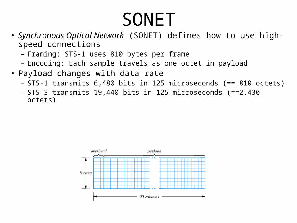
SONET• Synchronous Optical Network (SONET) defines how to use high-

speed connections – Framing: STS-1 uses 810 bytes per frame – Encoding: Each sample travels as one octet in payload

• Payload changes with data rate – STS-1 transmits 6,480 bits in 125 microseconds (== 810 octets) – STS-3 transmits 19,440 bits in 125 microseconds (==2,430 octets)

Getting To Your Home

• Local loop describes connection from telephone office to your home

• Sometimes called POTS (Plain Old Telephone Service) • Legacy infrastructure is copper

– ISDN, DSL

• Other available connections include – Cable TV

– Wireless

– Electric power

ISDN

• Integrated Services Digital Network• Provides digital service (like T-series) on existing local loop

copper • Three separate circuits, or channels

– Two B channels, 64 Kbps each; == 2 voice circuits – One D channel, 16 Kbps; control

• Often written as 2B+D; called Basic Rate Interface (BRI) • Slow to catch on

– Expensive – Charged by time used like POTS– (Almost) equaled by analog modems – Was required for some video conferencing apps

DSL

• DSL (Digital Subscriber Line) is a family of technologies – Sometimes called xDSL

– Provides high-speed digital service over existing local loop

• One common form is ADSL (Asymmetric DSL) – Higher speed into home than out of home

– More bits flow in ("downstream") than out ("upstream")

• ADSL maximum speeds: – 6.144 Mbps downstream

– 640 Kbps upstream

Adaptive Transmission

• Individual local loops have different transmission characteristics – Different maximum frequencies – Different interference frequencies

• ADSL uses FDM – 286 frequencies or channels, each 4Khz bandwidth

• 255 downstream • 31 upstream • 2 control

• Each frequency carries data independently – All frequencies out of audio range – Bit rate adapts to quality in each frequency

Other DSL’s

• SDSL (Symmetric DSL) provides divides frequencies evenly

• HDSL (High-rate DSL) provides DS1 bit rate both directions – Short distances – Four wires

• VDSL(Very high bit rate DSL) provides up to 52 Mbps – Very short distance – Requires Optical Network Unit (ONU) as a relay

Cable Modems• Cable TV already brings high bandwidth coax into your

house • Cable modems encode and decode data from cable TV

coax – One in cable TV center connects to network – One in home connects to computer

• Bandwidth multiplexed among all users over tree-based topology

• Multiple access medium; your neighbor can see your data! • Not all cable TV coax plants are bidirectional, makes

upstream more difficult– Originally only had amplifiers for downstream

Hybrid Fiber Coax

• HFC used to provide efficient two-way communications– Combination of optical fibers and coax, with fiber for central

facilities and coax to the individuals– Requires upgrade to network, replace feeder networks with

fiber to the trunk with fiber– Time division multiplexing– 50-450 Mhz for TV, 6Mhz per TV channel– 450-750 Mhz for downstream data– 5-50 Mhz for upstream data

Proxy/caching

Summary

• WAN links between sites use digital telephony – Based on digitized voice service – Several standard rates – Requires conversion vis DSU/CSU

• Local loop technologies – ISDN – xDSL – Cable modem – Satellite (already discussed previously)– Fiber to the curb (fiber boon seems to be ending now, so not too

likely)

WAN Technologies / Routing

• Here we’ll look at WAN technologies and an overview of how routing works in general

• We’ll see specific details on implementations of routing later

• Recall– LANs to MANs to WANs

– Need different technology to implement WANs then we have for LANs

– WAN must be scalable to long distances and many systems

Packet Switches

• To span long distances or many computers, network must replace shared medium with packet switches – Each switch moves an entire packet from one connection to another – A small computer with network interfaces, memory and program

dedicated to packet switching function – Packets switches may connect to computers and to other packet

switches – Typically high speed connections to other packets switches, lower

speed to computers – Technology details depend on desired speed

Switches as Building Blocks

• Packet switches can be linked together to form WANs

• WANs need not be symmetric or have regular connections

• Each switch may connect to one or more other switches and one or more computers

Store & Forward Switches

• Switches commonly use Store & Forward– Packet switch stores incoming packet

– ... and forwards the packet to another switch or computer

• Packet switch has internal memory – Can hold packet if outgoing connection is busy – Packets for each connection held on queue – This also lets us do things like error detection if we like,

and discard bad packets, unlike cut-through switches which only examine the headers and then forward the rest of the packet on

Physical Addressing in a WAN

• Similar to LAN – Data transmitted in packets (equivalent to frames) – Each packet has format with header – Packet header includes destination and source addresses

• Many WANs use hierarchical addressing for efficiency – One part of address identifies destination switch – Other part of address identifies port on switch

Next Hop Forwarding

• Packet switch must choose outgoing connection for forwarding – If destination is local computer, packet switch delivers

computer port – If destination is attached another switch, this packet

switch forwards to next hop through connection to another switch

• Choice based on destination address in packet

Next Hop Example• Packet switch doesn't keep complete information

about all possible destination – Just keeps next hop – So, for each packet, packet switch looks up

destination in table and forwards through connection to next hop

• Example for Switch 2

Source Independence

• Next hop to destination does not depend on source of packet

• Called source independence • Allows fast, efficient routing • Packet switch need not have complete

information, just next hop – Reduces total information – Increases dynamic robustness - network can continue

to function even if topology changes without notifying entire network

Routing

• Process of forwarding is called routing

• Information is kept in routing table

• Note that many entries have same next hop

• In particular, all destinations on same switch have same next hop

• Thus, routing table can be collapsed:

WAN Routing

• More computers == more traffic • Can add capacity to WAN by adding more links and

packet switches • Packet switches need not have computers attached • Interior switch - no attached computers • Exterior switch - attached computers

• Note: Interior and Exterior will have different meanings when we talk about routing across different networks; (interior == in our network, exterior == connected to outside network)

WAN Routing• Both interior and exterior switches:

– Forward packets – Need routing tables

• Must have: – Universal routing - next hop for each possible destination – Optimal routes - next hop in table must be on shortest path to destination

• Use a graph to model– Nodes model switches – Edges model direct connections between switches – Captures essence of network, ignoring attached computers

Routing Theory

Graph abstraction for routing algorithms:

graph nodes are routers

graph edges are physical links link cost: delay, $

cost, hops, or congestion level

Goal: determine “good” path

(sequence of routers) thru network from source to

dest.

A

ED

CB

F

2

2

13

1

1

2

53

5

• “good” path:– typically means

minimum cost path

– other def’s possible

Least cost path from A to C?

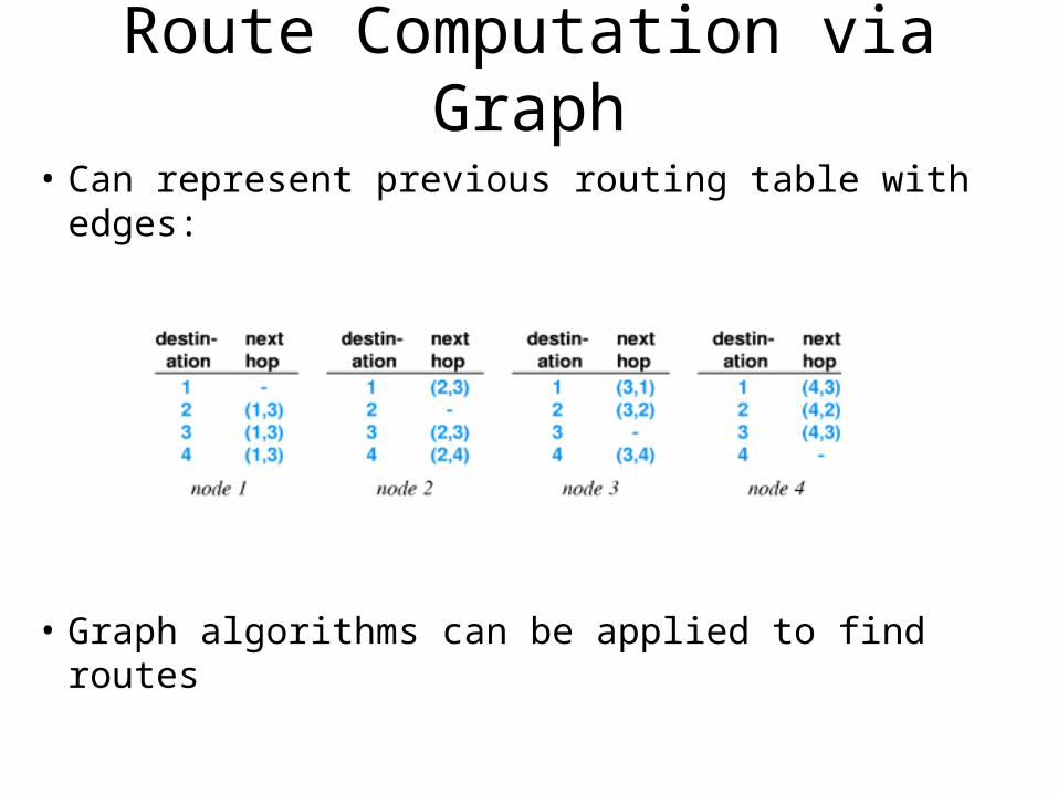
Route Computation via Graph

• Can represent previous routing table with edges:

• Graph algorithms can be applied to find routes

• Notice duplication of information in routing table for node 1:

• Switch 1 has only one outgoing connection; all traffic must traverse that connection

• Can collapse routing table entries with a default route

• If destination does not have an explicit routing table entry, use use the default route, specified by *

Redundant Routing Info

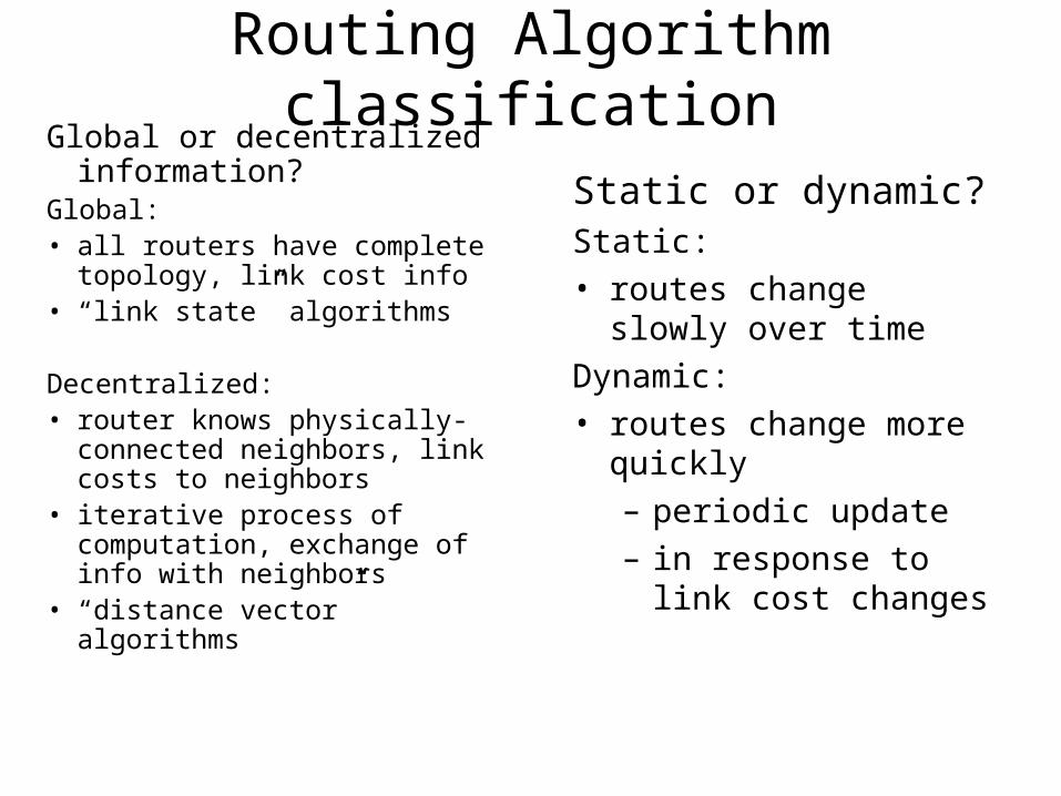
Routing Algorithm classificationGlobal or decentralized

information?Global:• all routers have complete

topology, link cost info• “link state” algorithms

Decentralized: • router knows physically-

connected neighbors, link costs to neighbors

• iterative process of computation, exchange of info with neighbors

• “distance vector” algorithms

Static or dynamic?Static:

• routes change slowly over time

Dynamic:

• routes change more quickly

– periodic update

– in response to link cost changes

A Link-State Routing Algorithm

Dijkstra’s algorithm• net topology, link costs known to all nodes

– accomplished via “link state broadcast” – all nodes have same info

• computes least cost paths from one node (‘source”) to all other nodes– gives routing table for that node

• iterative: after k iterations, know least cost path to k dest.’s

Dijkstra’s Algorithm

Dijkstra(G,w,s) ; Graph G, weights w, source s for each vertex vG, set d[v] and P[v] NIL d[s] 0 S{} QAll Vertices in G with associated d while Q not empty do uExtract-Min(Q) SS{u} for each vertex v Adj[u] do

if d[v]>d[u]+w(u,v) then d[v]d[u]+w(u,v) ; decrement distance

P[v] u ; indicate parent node

Dijkstra Example (0)

6

5

4

2

1

15

14

6

3 8

a

b c d

e f g

h

15 4

Dijkstra Example 1

Extract min, vertex f. S={f}. Update shorter paths.

6

5

4

2

1

15

14

6

3 8

a

b c d

e f g

h

15 4

Initialize nodes to , parent to nil. S={}, Q={(a,) (b,) (c, ) (d, ) (e, ) (f,0) (g, ) (h, )}

INF,NIL

INF,NIL

INF,NIL

INF,NIL

0,NIL

INF,NIL INF,NIL

INF,NIL

Dijkstra Example 2

Extract min, vertex c. S={fc}. Update shorter paths.

6

5

4

2

1

15

14

6

3 8

a

b c d

e f g

h

15 4

15,f

INF,NIL

INF,NIL

0,NIL

2,f 4,f

15,f

Q={(a,) (b,15) (c, 2) (d, 4) (e, ) (g, 15) (h, )} INF,NIL

Dijkstra Example 3

Extract min, vertex d. S={fcd}. Update shorter paths (None)

6

5

4

2

1

15

14

6

3 8

a

b c d

e f g

h

15 4

7,c

INF,NIL

INF,NIL

0,NIL

2,f 3,c

15,f

4,cQ={(a,6) (b,7) (d, 3) (e, ) (g, 15) (h, )}

Dijkstra Example 4

6

5

4

2

1

15

14

6

3 8

a

b c d

e f g

h

15 4

7,c

INF,NIL

INF,NIL

0,NIL

2,f 3,c

15,f

Extract min, vertex a. S={fcda}. Update shorter paths (None)Extract min, vertex b. S={fcdab}. Update shorter paths.

4,c

Dijkstra Example 5

Extract min, vertex h. S={fcdabh}. Update shorter paths

6

5

4

2

1

15

14

6

3 8

a

b c d

e f g

h

15 4

7,c

INF,NIL

13,c

0,NIL

2,f 3,c

15,f

4,c

Q={ (e, ) (g, 15) (h, 13)}

Dijkstra Example 6

Extract min, vertex g and h – nothing to update, done!

6

5

4

2

1

15

14

6

3 8

a

b c d

e f g

h

15 4

7,c

16,h

13,c

0,NIL

2,f 3,c

15,f

4,c

Q={ ( (e, 16) (g, 15) }

Dijkstra Example 7

• Can follow parent “pointers” to get the path

6

5

4

2

1

15

14

6

3 8

a

b c d

e f g

h

15 4

7,c

16,h

13,c

0,NIL

2,f 3,c

15,f

4,c

Dijkstra’s algorithm, discussion

Algorithm complexity: n nodes• each iteration: need to check all nodes• n*(n+1)/2 comparisons: O(n2) - using linear array for Q• more efficient implementations possible: O(nlgn) – using min heap for Q

Oscillations possible for some pathological cases:• e.g., link cost = amount of carried traffic• Possible solutions?

A

D

C

B1 1+e

e0

e

1 1

0 0

A

D

C

B2+e 0

001+e1

A

D

C

B0 2+e

1+e10 0

A

D

C

B2+e 0

e01+e1

Initiallyctr-clockwise

… recomputerouting

clockwise

… recomputectr-clockwise

… recomputeclockwise

Distance Vector Routing Algorithm

iterative:• continues until no nodes

exchange info.• self-terminating: no

“signal” to stop

asynchronous:• nodes need not exchange

info/iterate in lock step!distributed:• each node communicates

only with directly-attached neighbors

Distance Table data structure • each node has its own• row for each possible destination• column for each directly-attached

neighbor to node• example: in node X, for dest. Y via

neighbor Z:

D (Y,Z)X

distance from X toY, via Z as next hop

cost(X,Z) + min {D (Y,w)} Z

w

=

=

Distance Table: example

A

E D

CB7

8

1

2

1

2

D ()

A

B

C

D

A

1

7

6

4

B

14

8

9

11

D

5

5

4

2

Ecost to destination via

dest

inat

ion

D (C,D)E

c(E,D) + min {D (C,w)}D

w== 2+2 = 4

D (A,D)E

c(E,D) + min {D (A,w)}D

w== 2+3 = 5

D (A,B)E

c(E,B) + min {D (A,w)}B

w== 8+6 = 14

loop!

loop!

Distance table gives routing table

D ()

A

B

C

D

A

1

7

6

4

B

14

8

9

11

D

5

5

4

2

Ecost to destination via

dest

inat

ion

A

B

C

D

A,1

D,5

D,4

D,2

Outgoing link to use, cost

dest

inat

ion

Distance table Routing table

Distance Vector Routing: overview

Iterative, asynchronous: each local iteration caused by:

• local link cost change • message from neighbor: its

least cost path change from neighbor

Distributed:• each node notifies neighbors

only when its least cost path to any destination changes– neighbors then notify their

neighbors if necessary

wait for (change in local link cost of msg from neighbor)

recompute distance table

if least cost path to any dest

has changed, notify neighbors

Each node:

Distance Vector Algorithm:

1 Initialization: 2 for all adjacent nodes v: 3 D (*,v) = infty /* the * operator means "for all rows" */ 4 D (v,v) = c(X,v) 5 for all destinations, y 6 send min D (y,w) to each neighbor /* w over all X's neighbors */

XX

Xw

At all nodes, X:

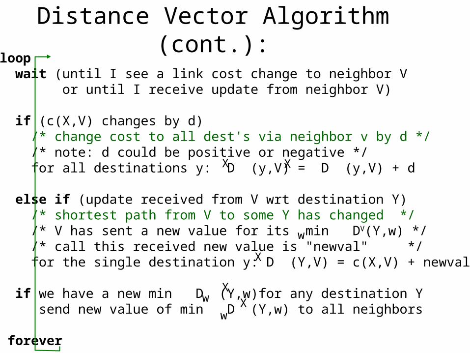
Distance Vector Algorithm (cont.):8 loop 9 wait (until I see a link cost change to neighbor V 10 or until I receive update from neighbor V) 11 12 if (c(X,V) changes by d) 13 /* change cost to all dest's via neighbor v by d */ 14 /* note: d could be positive or negative */ 15 for all destinations y: D (y,V) = D (y,V) + d 16 17 else if (update received from V wrt destination Y) 18 /* shortest path from V to some Y has changed */ 19 /* V has sent a new value for its min DV(Y,w) */ 20 /* call this received new value is "newval" */ 21 for the single destination y: D (Y,V) = c(X,V) + newval 22 23 if we have a new min D (Y,w)for any destination Y 24 send new value of min D (Y,w) to all neighbors 25 26 forever

w

XX

XX

X

w

w

Distance Vector Algorithm: example

X Z12

7

Y

Distance Vector Algorithm: example

X Z12

7

Y

D (Y,Z)X

c(X,Z) + min {D (Y,w)}w=

= 7+1 = 8

Z

D (Z,Y)X

c(X,Y) + min {D (Z,w)}w=

= 2+1 = 3

Y

Distance Vector: link cost changes

Link cost changes:• node detects local link cost change

• updates distance table (line 15)

• if cost change in least cost path, notify neighbors (lines 23,24)

X Z14

50

Y1

algorithmterminates“good

news travelsfast”

How could a link get shorter?

Distance Vector: link cost changes

Link cost changes:• good news travels fast • bad news travels slow - “count

to infinity” problem!X Z

14

50

Y60

algorithmcontinues

on!

44 iter!

Comparison of LS and DV algorithms

Message complexity• LS: with n nodes, E links, O(nE)

msgs sent each • DV: exchange between

neighbors only– convergence time varies

Speed of Convergence• LS: O(n2) algorithm requires

O(nE) msgs– may have oscillations

• DV: convergence time varies– may be routing loops– count-to-infinity problem

Robustness: what happens if router malfunctions?

LS: – node can advertise incorrect

link cost– each node computes only its

own table

DV:– DV node can advertise

incorrect path cost– each node’s table used by

others • error propagate thru network• Could cause a flood

Routing Implementation

• Link State (Dijkstra’s Algorithm)– Used in OSPF

• Distance Vector (Bellman-Ford Algorithm)– Used in Internet BGP, IPX, RIP

Examples of WAN Technology

• ARPANET – Original precursor to the ‘Net

• X.25 – Early standard for connection-oriented networking – From ITU, which was originally CCITT – Predates computer connections, used for terminal/timesharing

connection

• Frame Relay – Telco service for delivering blocks of data – Connection-based service; must contract with telco for circuit

between two endpoints – Typically 56Kbps or 1.5Mbps; can run to 100Mbps

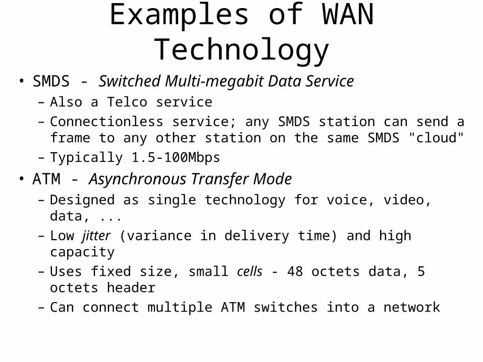
Examples of WAN Technology

• SMDS - Switched Multi-megabit Data Service – Also a Telco service

– Connectionless service; any SMDS station can send a frame to any other station on the same SMDS "cloud"

– Typically 1.5-100Mbps

• ATM - Asynchronous Transfer Mode – Designed as single technology for voice, video, data, ...

– Low jitter (variance in delivery time) and high capacity

– Uses fixed size, small cells - 48 octets data, 5 octets header

– Can connect multiple ATM switches into a network

Summary

• WAN can span arbitrary distances and interconnect arbitrarily many computers

• Uses packet switches and point-to-point connections • Packets switches use store-and-forward and routing

tables to deliver packets to destination • WANs use hierarchical addressing • Graph algorithms can be used to compute routing tables • Many LAN technologies exist