1

Wannier-Stark resonances in optical and

semiconductor superlattices

Markus Glucka, Andrey R. Kolovskyab, and Hans Jurgen Korscha

aFB Physik, Universitat Kaiserslautern, D-67653 Kaiserslautern, Germany

bL. V. Kirensky Institute of Physics, 660036 Krasnoyarsk, Russia

Abstract:In this work, we discuss the resonance states of a quantum particle in a periodic potential plusa static force. Originally this problem was formulated for a crystal electron subject to a staticelectric field and it is nowadays known as the Wannier-Stark problem. We describe a novelapproach to the Wannier-Stark problem developed in recent years. This approach allows tocompute the complex energy spectrum of a Wannier-Stark system as the poles of a rigorouslyconstructed scattering matrix and solves the Wannier-Stark problem without any approximation.The suggested method is very efficient from the numerical point of view and has proven to bea powerful analytic tool for Wannier-Stark resonances appearing in different physical systemssuch as optical lattices or semiconductor superlattices.

PACS: 03.65.-w; 05.45.+b; 32.80.Pj; -73.20.Dx

Contents

1 Introduction 41.1 Wannier-Stark problem . . . . . . . . . . . . . . . . . . . . . . . . . . . . . . . . 41.2 Tight-binding model . . . . . . . . . . . . . . . . . . . . . . . . . . . . . . . . . . 61.3 Landau-Zener tunneling . . . . . . . . . . . . . . . . . . . . . . . . . . . . . . . . 81.4 Experimental realizations . . . . . . . . . . . . . . . . . . . . . . . . . . . . . . . 91.5 This work . . . . . . . . . . . . . . . . . . . . . . . . . . . . . . . . . . . . . . . . 11

2 Scattering theory for Wannier-Stark systems 132.1 S-matrix and Floquet-Bloch operator . . . . . . . . . . . . . . . . . . . . . . . . . 132.2 S-matrix: basic equations . . . . . . . . . . . . . . . . . . . . . . . . . . . . . . . 162.3 Calculating the poles of the S-matrix . . . . . . . . . . . . . . . . . . . . . . . . . 182.4 Resonance eigenfunctions . . . . . . . . . . . . . . . . . . . . . . . . . . . . . . . 20

3 Interaction of Wannier-Stark ladders 243.1 Resonant tunneling . . . . . . . . . . . . . . . . . . . . . . . . . . . . . . . . . . . 243.2 Two interacting Wannier-Stark ladders . . . . . . . . . . . . . . . . . . . . . . . . 273.3 Wannier-Stark ladders in optical lattices . . . . . . . . . . . . . . . . . . . . . . . 283.4 Wannier-Stark ladders in semiconductor superlattices . . . . . . . . . . . . . . . 30

4 Spectroscopy of Wannier-Stark ladders 334.1 Decay spectrum and Fermi’s golden rule . . . . . . . . . . . . . . . . . . . . . . . 334.2 Dipole matrix elements . . . . . . . . . . . . . . . . . . . . . . . . . . . . . . . . . 354.3 Decay spectra for atoms in optical lattices . . . . . . . . . . . . . . . . . . . . . . 384.4 Absorption spectra of semiconductor superlattices . . . . . . . . . . . . . . . . . 42

5 Quasienergy Wannier-Stark states 445.1 Single-band quasienergy spectrum . . . . . . . . . . . . . . . . . . . . . . . . . . 445.2 S-matrix for time-dependent potentials . . . . . . . . . . . . . . . . . . . . . . . . 475.3 Complex quasienergy spectrum . . . . . . . . . . . . . . . . . . . . . . . . . . . . 505.4 Perturbation theory for rational frequencies . . . . . . . . . . . . . . . . . . . . . 525.5 Selective decay . . . . . . . . . . . . . . . . . . . . . . . . . . . . . . . . . . . . . 54

6 Wave packet dynamics 586.1 Expansion over resonance states . . . . . . . . . . . . . . . . . . . . . . . . . . . 58

2

3

6.2 Pulse output from Wannier-Stark systems . . . . . . . . . . . . . . . . . . . . . . 616.3 Atom laser mode-locking . . . . . . . . . . . . . . . . . . . . . . . . . . . . . . . . 63

7 Chaotic scattering 677.1 Classical dynamics . . . . . . . . . . . . . . . . . . . . . . . . . . . . . . . . . . . 687.2 Irregular quasienergy spectrum . . . . . . . . . . . . . . . . . . . . . . . . . . . . 717.3 Random matrix model . . . . . . . . . . . . . . . . . . . . . . . . . . . . . . . . . 757.4 Resonance statistics . . . . . . . . . . . . . . . . . . . . . . . . . . . . . . . . . . 777.5 Fractional stabilization . . . . . . . . . . . . . . . . . . . . . . . . . . . . . . . . . 80

8 Conclusions and outlook 84

Chapter 1

Introduction

The problem of a Bloch particle in the presence of additional external fields is as old as thequantum theory of solids. Nevertheless, the topics introduced in the early studies of the system,Bloch oscillations [ 1], Zener tunneling [ 2] and the Wannier-Stark ladder [ 3], are still thesubject of current research. The literature on the field is vast and manifold, with different,sometimes unconnected lines of evolution. In this introduction we try to give a survey of thefield, summarize the different theoretical approaches and discuss the experimental realizationsof the system. It should be noted from the very beginning that most of the literature deals withone-dimensional single-particle descriptions of the system, which, however, capture the essentialphysics of real systems. Indeed, we will also work in this context.

1.1. Wannier-Stark problem

In the one-dimensional case the Hamiltonian of a Bloch particle in an additional external field,in the following referred to as the Wannier-Stark Hamiltonian, has the form

HW =p2

2m+ V (x) + Fx, V (x+ d) = V (x), (1.1)

where F stands for the static force induced by the external field. Clearly, the external fielddestroys the translational symmetry of the field-free Hamiltonian H0 = p2/2m+ V (x). Instead,from an arbitrary eigenstate with HWΨ = E0Ψ, one can by a translation over l periods dconstruct a whole ladder of eigenstates with energies El = E0 + ldF , the so-called Wannier-Starkladder. Any superposition of these states has an oscillatory evolution with the time period

TB =2π~dF

, (1.2)

known as the Bloch period. There has been a long-standing controversy about the existence ofthe Wannier-Stark ladder and Bloch oscillations [ 4, 5, 6, 7, 8, 9, 10, 11, 12, 13, 14, 15, 16, 17,18, 19], and only recently agreement about the nature of the Wannier-Stark ladder was reached.The history of this discussion is carefully summarized in [ 12, 20, 21, 22].

From today’s point of view the discussion mainly dealt with the effect of the single bandapproximation (effectively a projection on a subspace of the Hilbert space) on the spectralproperties of the Wannier-Stark Hamiltonian. Within the single band approximation, the α’th

4

5

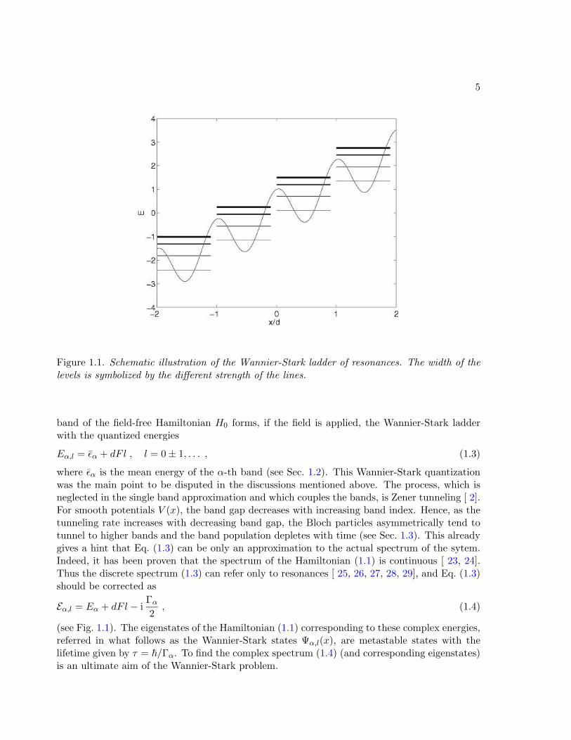
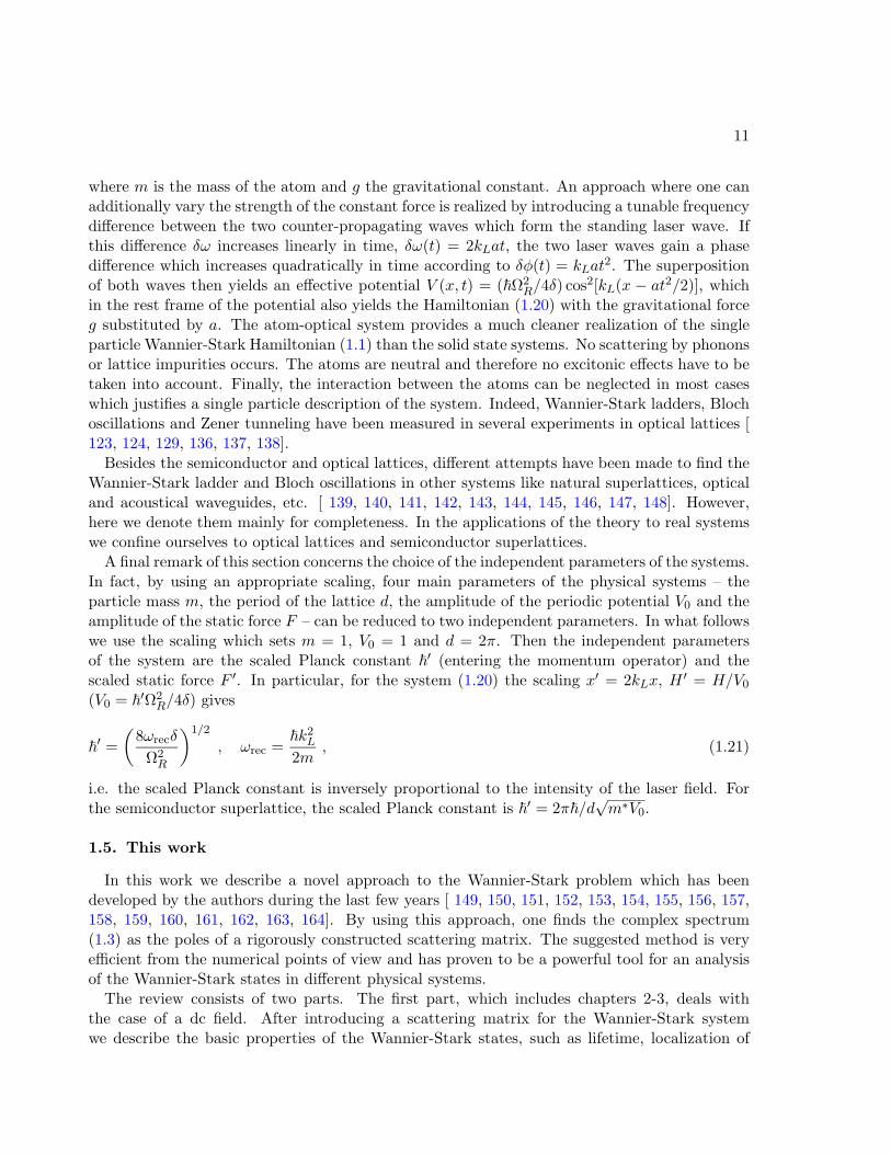
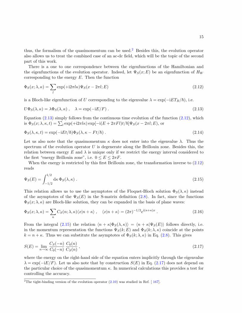
Figure 1.1. Schematic illustration of the Wannier-Stark ladder of resonances. The width of thelevels is symbolized by the different strength of the lines.

band of the field-free Hamiltonian H0 forms, if the field is applied, the Wannier-Stark ladderwith the quantized energies

Eα,l = εα + dF l , l = 0± 1, . . . , (1.3)

where εα is the mean energy of the α-th band (see Sec. 1.2). This Wannier-Stark quantizationwas the main point to be disputed in the discussions mentioned above. The process, which isneglected in the single band approximation and which couples the bands, is Zener tunneling [ 2].For smooth potentials V (x), the band gap decreases with increasing band index. Hence, as thetunneling rate increases with decreasing band gap, the Bloch particles asymmetrically tend totunnel to higher bands and the band population depletes with time (see Sec. 1.3). This alreadygives a hint that Eq. (1.3) can be only an approximation to the actual spectrum of the sytem.Indeed, it has been proven that the spectrum of the Hamiltonian (1.1) is continuous [ 23, 24].Thus the discrete spectrum (1.3) can refer only to resonances [ 25, 26, 27, 28, 29], and Eq. (1.3)should be corrected as

Eα,l = Eα + dF l − iΓα2, (1.4)

(see Fig. 1.1). The eigenstates of the Hamiltonian (1.1) corresponding to these complex energies,referred in what follows as the Wannier-Stark states Ψα,l(x), are metastable states with thelifetime given by τ = ~/Γα. To find the complex spectrum (1.4) (and corresponding eigenstates)is an ultimate aim of the Wannier-Stark problem.

6

Several attempts have been made to calculate the Wannier-Stark ladder of resonances. Someanalytical results have been obtained for nonlocal potentials [ 30, 31] and for potentials with afinite number of gaps [ 32, 33, 34, 35, 36, 37, 38]. (We note, however, that almost all periodicpotentials have an infinite number of gaps.) A common numerical approach is the formalismof a transfer matrix to potentials which consist of piecewise constant or linear parts, eventuallyseparated by delta function barriers [ 39, 40, 41, 42, 43]. Other methods approximate theperiodic system by a finite one [ 44, 45, 46, 47]. Most of the results concerning Wannier-Stark systems, however, have been deduced from single- or finite-band approximations andstrongly related tight-binding models. The main advantage of these models is that they, aswell in the case of static (dc) field [ 48] as in the cases of oscillatory (ac) and dc-ac fields[ 49, 50, 51, 52, 53, 54, 55, 56], allow analytical solutions. Tight-binding models have beenadditionally used to investigate the effect of disorder [ 57, 58, 59, 60, 61, 62], noise [ 63] oralternating site energies [ 64, 65, 66, 67, 68] on the dynamics of Bloch particles in externalfields. In two-band descriptions Zener tunneling has been studied [ 69, 70, 71, 72, 73], whichleads to Rabi oscillations between Bloch bands [ 74]. Because of the importance of tight-bindingand single-band models for understanding the properties of Wannier-Stark resonances we shalldiscuss them in some more detail.

1.2. Tight-binding model

In a simple way, the tight-binding model can be introduced by using the so-called Wannierstates (not to be confused with Wannier-Stark states), which are defined as follows. In theabsence of a static field, the eigenstates of the field-free Hamiltonian,

H0 =p2

2m+ V (x) , (1.5)

are known to be the Bloch waves

φα,κ(x) = exp(iκx)χα,κ(x) , χα,κ(x+ d) = χα,κ(x) , (1.6)

with the quasimomentum κ defined in the first Brillouin zone −π/d ≤ κ < π/d. The functions(1.6) solve the eigenvalue equation

H0φα,κ(x) = εα(κ)φα,κ(x) , εα(κ+ 2π/d) = εα(κ) , (1.7)

where εα(κ) are the Bloch bands. Without affecting the energy spectrum, the free phase of theBloch function φα,κ(x) can be chosen such that it is an analytic and periodic function of thequasimomentum κ [ 75]. Then we can expand it in a Fourier series in κ, where the expansioncoefficients

ψα,l(x) =∫ π/d

−π/ddκ exp(−iκld)φα,κ(x) (1.8)

are the Wannier functions.Let us briefly recall the main properties of the Wannier and Bloch states. Both form orthogonal

sets with respect to both indices. The Bloch functions are, in general, complex while the Wannierfunctions can be chosen to be real. While the Bloch states are extended over the whole coordinate

7

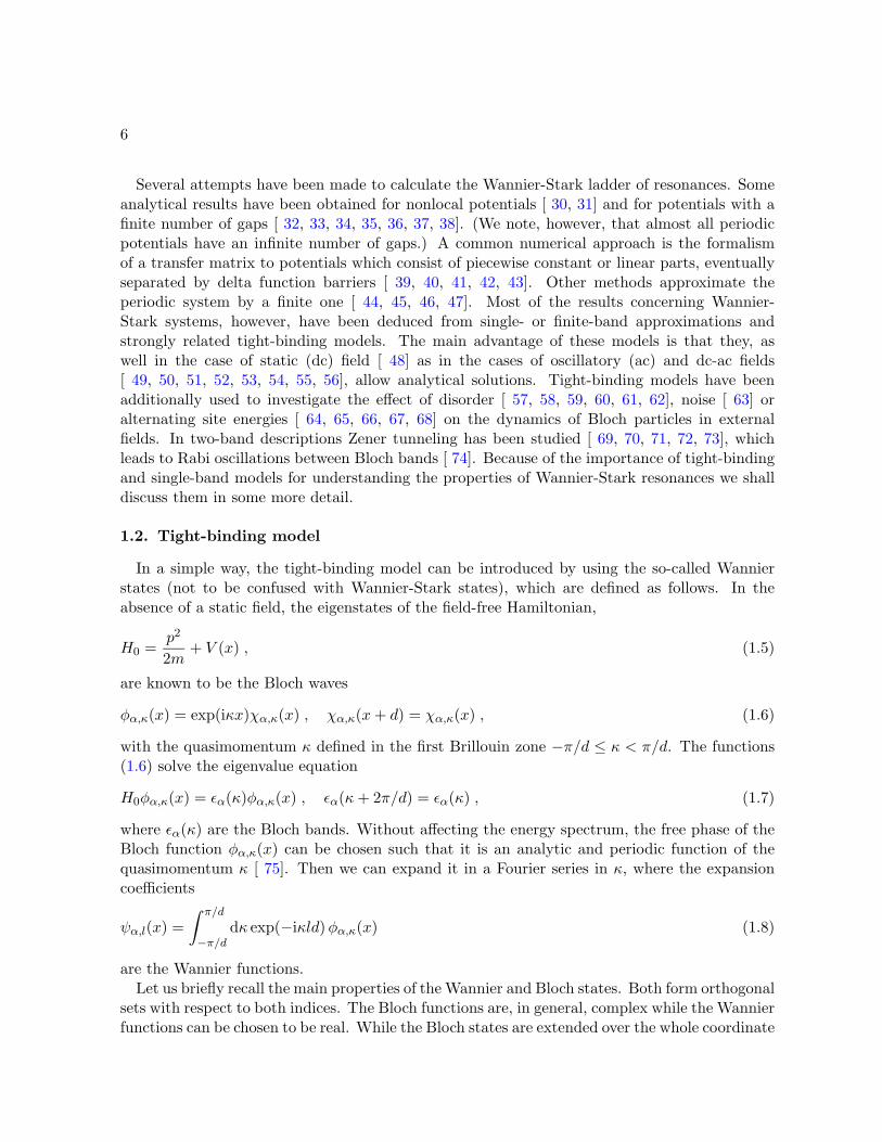
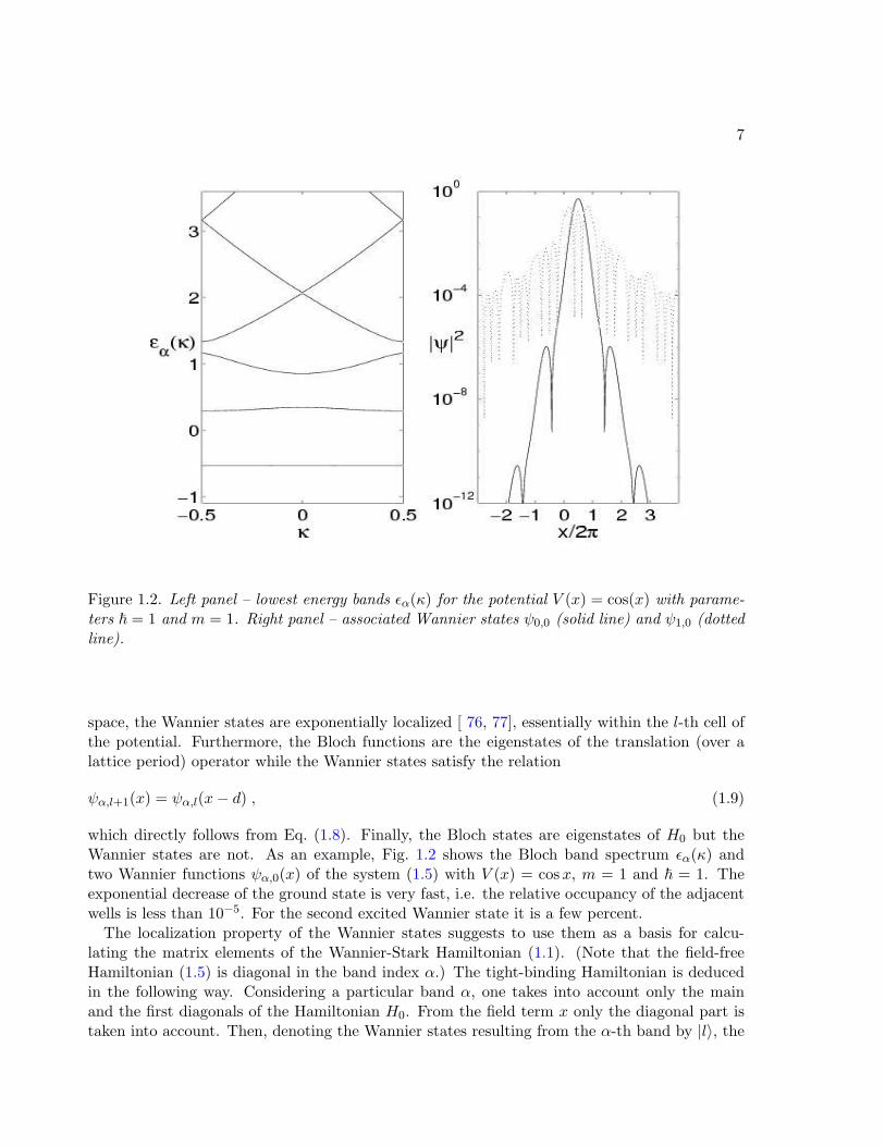
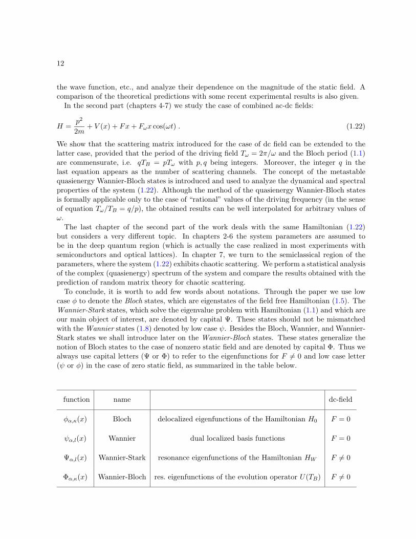
Figure 1.2. Left panel – lowest energy bands εα(κ) for the potential V (x) = cos(x) with parame-ters ~ = 1 and m = 1. Right panel – associated Wannier states ψ0,0 (solid line) and ψ1,0 (dottedline).

space, the Wannier states are exponentially localized [ 76, 77], essentially within the l-th cell ofthe potential. Furthermore, the Bloch functions are the eigenstates of the translation (over alattice period) operator while the Wannier states satisfy the relation

ψα,l+1(x) = ψα,l(x− d) , (1.9)

which directly follows from Eq. (1.8). Finally, the Bloch states are eigenstates of H0 but theWannier states are not. As an example, Fig. 1.2 shows the Bloch band spectrum εα(κ) andtwo Wannier functions ψα,0(x) of the system (1.5) with V (x) = cosx, m = 1 and ~ = 1. Theexponential decrease of the ground state is very fast, i.e. the relative occupancy of the adjacentwells is less than 10−5. For the second excited Wannier state it is a few percent.

The localization property of the Wannier states suggests to use them as a basis for calcu-lating the matrix elements of the Wannier-Stark Hamiltonian (1.1). (Note that the field-freeHamiltonian (1.5) is diagonal in the band index α.) The tight-binding Hamiltonian is deducedin the following way. Considering a particular band α, one takes into account only the mainand the first diagonals of the Hamiltonian H0. From the field term x only the diagonal part istaken into account. Then, denoting the Wannier states resulting from the α-th band by |l〉, the

8

tight-binding Hamiltonian reads

HTB =∑l

(εα + dF l) |l〉〈l|+ ∆α

4( |l + 1〉〈l|+ |l〉〈l + 1| ) . (1.10)

The Hamiltonian (1.10) can be easily diagonalized which yields the spectrum Eα,l = εα + dF lwith the eigenstates

|Ψα,l〉 =∑m

Jm−l

( ∆α

2dF

)|m〉 . (1.11)

Thus, all states are localized and the spectrum is the discrete Wannier-Stark ladder (1.3).The obtained result has a transparent physical meaning. When F = 0 the energy levels of

Wannier states |l〉 coincide and the tunneling couples them into Bloch waves |κ〉 =∑

l exp(iκl)|l〉.Correspondingly, the infinite degeneracy of the level εα is removed, producing the Bloch bandεα(κ) = εα + (∆α/2) cos(dκ).1 When F 6= 0 the Wannier levels are misaligned and the tunnelingis suppressed. As a consequence, the Wannier-Stark state involves (effectively) a finite numberof Wannier states, as indicated by Eq. (1.11). It will be demonstrated later on that for thelow-lying bands Eq. (1.3) and Eq. (1.11) approximate quite well the real part of the complexWannier-Stark spectrum and the resonance Wannier-Stark functions Ψα,l(x), respectively. Themain drawback of the model, however, is its inability to predict the imaginary part of thespectrum (i.e. the lifetime of the Wannier-Stark states), which one has to estimate from anindependent calculation. Usually this is done with the help of Landau-Zener theory.

1.3. Landau-Zener tunneling

Let us address the following question: if we take an initial state in the form of a Bloch wavewith quasimomentum κ, what will be the time evolution of this state when the external staticfield is switched on?

The common approach to this problem is to look for the solution as the superposition ofHouston functions [ 78]

ψ(x, t) =∑α

cα(t)ψα(x, t) , (1.12)

ψα(x, t) = exp(− i~

∫ t

0dt′εα(κ′)

)φα,κ′(x) , (1.13)

where φα,κ′(x) is the Bloch function with the quasimomentum κ′ evolving according to theclassical equation of motion p = −F , i.e κ′ = κ − Ft/~. Substituting Eq. (1.12) into thetime-dependent Schrodinger equation with the Hamiltonian (1.1), we obtain

i~ cα = F∑β

Xα,β(κ′) exp(− i~

∫ t

0dt′[εα(κ′)− εβ(κ′)]

)cβ , (1.14)

1Because only the nearest off-diagonal elements are taken into account in Eq. (1.10), the Bloch bands are alwaysapproximated by a cosine dispersion relation.

9

where Xα,β(κ) = i∫

dxχ∗α,κ(x) ∂/∂κXβ,κ(x). Neglecting the interband coupling, i.e. Xα,β = 0for α 6= β, we have

cβ(t) ≈ 0 for α 6= β and i~ cα = F Xα,α(κ′) cα . (1.15)

This solution is the essence of the so-called single-band approximation. We note that within thisapproximation one can use the Houston functions (1.13) to construct the localized Wannier-Starkstates similar to those obtained with the help of the tight-binding model.

The correction to the solution (1.15) is obtained by using the formalism of Landau-Zenertunneling. In fact, when the quasimomentum κ′ explores the Brillouin zone, the adiabatictransition occurs at the points of “avoided” crossings between the adjacent Bloch bands [see,for example, the avoided crossing between the 4-th and 5-th bands in Fig. 1.2(a) at κ = 0].Semiclassically, the probability of this transition is given by

P ≈ exp

(−

π∆2α,β

8~(|ε′α|+ |ε′β|)F

), (1.16)

where ∆α,β is the energy gap between the bands and ε′α, ε′β stand for the slope of the bandsat the point of avoided crossing in the limit ∆α,β → 0 [ 79]. In a first approximation, one canassume that the adiabatic transition occurs once for each Bloch cycle TB = 2π~/dF . Then thepopulation of the α-th band decreases exponentially with the decay time

τ = ~/Γα , Γα = aαF exp(−bα/F ) , (1.17)

where aα and bα are band-dependent constants.In conclusion, within the approach described above one obtains from each Bloch band a set

of localized states with energies given by Eq. (1.3). However, these states have a finite lifetimegiven by Eq. (1.17). It will be shown in Sec. 3.1 that the estimate (1.17) is, in fact, a good “firstorder” approximation for the lifetime of the metastable Wannier-Stark states.

1.4. Experimental realizations

We proceed with experimental realizations of the Wannier-Stark Hamiltonian (1.1). Originally,the problem was formulated for a solid state electron system with an applied external electricfield, and in fact, the first measurements concerning the existence of the Wannier-Stark ladderdealt with photo-absorption in crystals [ 80]. Although this system seems convenient at firstglance, it meets several difficulties because of the intrinsic multi-particle character of the system.Namely, the dynamics of an electron in a solid is additionally influenced by electron-phonon andelectron-electron interactions. In addition, scattering by impurities has to be taken into account.In fact, for all reasonable values of the field, the Bloch time (1.2) is longer than the relaxationtime, and therefore neither Bloch oscillations nor Wannier-Stark ladders have been observed insolids yet.

One possibility to overcome these problems is provided by semiconductor superlattices [ 81],which consists of alternating layers of different semiconductors, as for example, GaAs andAlxGa1−xAs. In the most simple approach, the wave function of a carrier (electron or hole)in the transverse direction of the semiconductor superlattice is approximated by a plane wave

10

for a particle of mass m∗ (the effective mass of the electron in the conductance or valence bands,respectively). In the direction perpendicular to the semiconductor layers (let it be x-axis) thecarrier “sees” a periodic sequence of potential barriers

V (x) =V0 if ∃ l ∈ Z with |x− ld| < a/20 , else

, (1.18)

where the height of the barrier V0 is of the order of 100 meV and the period d ∼ 100 A. Becausethe period of this potential is two orders of magnitude larger than the lattice period in bulksemiconductor, the Bloch time is reduced by this factor and may be smaller than the relaxationtime. Indeed, semiconductor superlattices were the first systems where Wannier-Stark ladderswere observed [ 82, 83, 84] and Bloch oscillations have been measured in four-wave-mixingexperiments [ 85, 86] as proposed in [ 87]. In the following years, many facets of the topics havebeen investigated. Different methods for the observation of Bloch oscillation have been applied[ 88, 89, 90, 91], and nowadays it is possible to detect Bloch oscillations at room temperature [92], to directly measure [ 93] or even control [ 94] their amplitude. Wannier-Stark ladders havebeen found in a variety of superlattice structures [ 95, 96, 97, 98, 99], with different methods [100, 101]. The coupling between different Wannier-Stark ladders [ 102, 103, 104, 105, 106], theinfluence of scattering [ 107, 108, 109], the relation to the Franz-Keldysh effect [ 110, 111, 112],the influence of excitonic interactions [ 113, 114, 115, 116, 117] and the role of Zener tunneling[ 118, 119, 120, 121] have been investigated. Altogether, there is a large variety of interactionswhich affect the dynamics of the electrons in semiconductor superlattices, and it is still quitecomplicated to assign which effect is due to which origin.

A second experimental realization of the Wannier-Stark Hamiltonian is provided by cold atomsin optical lattices. The majority of experiments with optical lattices deals with neutral alkaliatoms such as lithium [ 122], sodium [ 123, 124, 125], rubidium [ 126, 127, 128] or cesium [129, 130, 131], but also optical lattices for argon have been realized [ 132]. The description ofthe atoms in an optical lattice is rather simple. One approximately treats the atom as a two-state system which is exposed to a strongly detuned standing laser wave. Then the light-inducedforce on the atom is described by the potential [ 133, 134]

V (x) =~Ω2

R

4δcos2(kLx) , (1.19)

where ~ΩR is the Rabi frequency (which is proportional to the product of the dipole matrixelements of the optical transition and the amplitude of the electric component of the laser field),kL is the wave number of the laser, and δ is the detuning of the laser frequency from the frequencyof the atomic transition.2

In addition to the optical forces, the gravitational force acts on the atoms. Therefore, a laseraligned in vertical direction yields the Wannier-Stark Hamiltonian

H =p2

2m+~Ω2

R

8δcos(2kLx) +mgx , (1.20)

2 The atoms are additionally exposed to dissipative forces, which may have substantial effects on the dynamics [135]. However, since these forces are proportional to δ−2 while the dipole force (1.19) is proportional to δ−1, forsufficiently large detuning one can reach the limit of non-dissipative optical lattices.

11

where m is the mass of the atom and g the gravitational constant. An approach where one canadditionally vary the strength of the constant force is realized by introducing a tunable frequencydifference between the two counter-propagating waves which form the standing laser wave. Ifthis difference δω increases linearly in time, δω(t) = 2kLat, the two laser waves gain a phasedifference which increases quadratically in time according to δφ(t) = kLat

2. The superpositionof both waves then yields an effective potential V (x, t) = (~Ω2

R/4δ) cos2[kL(x − at2/2)], whichin the rest frame of the potential also yields the Hamiltonian (1.20) with the gravitational forceg substituted by a. The atom-optical system provides a much cleaner realization of the singleparticle Wannier-Stark Hamiltonian (1.1) than the solid state systems. No scattering by phononsor lattice impurities occurs. The atoms are neutral and therefore no excitonic effects have to betaken into account. Finally, the interaction between the atoms can be neglected in most caseswhich justifies a single particle description of the system. Indeed, Wannier-Stark ladders, Blochoscillations and Zener tunneling have been measured in several experiments in optical lattices [123, 124, 129, 136, 137, 138].

Besides the semiconductor and optical lattices, different attempts have been made to find theWannier-Stark ladder and Bloch oscillations in other systems like natural superlattices, opticaland acoustical waveguides, etc. [ 139, 140, 141, 142, 143, 144, 145, 146, 147, 148]. However,here we denote them mainly for completeness. In the applications of the theory to real systemswe confine ourselves to optical lattices and semiconductor superlattices.

A final remark of this section concerns the choice of the independent parameters of the systems.In fact, by using an appropriate scaling, four main parameters of the physical systems – theparticle mass m, the period of the lattice d, the amplitude of the periodic potential V0 and theamplitude of the static force F – can be reduced to two independent parameters. In what followswe use the scaling which sets m = 1, V0 = 1 and d = 2π. Then the independent parametersof the system are the scaled Planck constant ~′ (entering the momentum operator) and thescaled static force F ′. In particular, for the system (1.20) the scaling x′ = 2kLx, H ′ = H/V0

(V0 = ~′Ω2R/4δ) gives

~′ =

(8ωrecδ

Ω2R

)1/2

, ωrec =~k2

L

2m, (1.21)

i.e. the scaled Planck constant is inversely proportional to the intensity of the laser field. Forthe semiconductor superlattice, the scaled Planck constant is ~′ = 2π~/d

√m∗V0.

1.5. This work

In this work we describe a novel approach to the Wannier-Stark problem which has beendeveloped by the authors during the last few years [ 149, 150, 151, 152, 153, 154, 155, 156, 157,158, 159, 160, 161, 162, 163, 164]. By using this approach, one finds the complex spectrum(1.3) as the poles of a rigorously constructed scattering matrix. The suggested method is veryefficient from the numerical points of view and has proven to be a powerful tool for an analysisof the Wannier-Stark states in different physical systems.

The review consists of two parts. The first part, which includes chapters 2-3, deals withthe case of a dc field. After introducing a scattering matrix for the Wannier-Stark systemwe describe the basic properties of the Wannier-Stark states, such as lifetime, localization of

12

the wave function, etc., and analyze their dependence on the magnitude of the static field. Acomparison of the theoretical predictions with some recent experimental results is also given.

In the second part (chapters 4-7) we study the case of combined ac-dc fields:

H =p2

2m+ V (x) + Fx+ Fωx cos(ωt) . (1.22)

We show that the scattering matrix introduced for the case of dc field can be extended to thelatter case, provided that the period of the driving field Tω = 2π/ω and the Bloch period (1.1)are commensurate, i.e. qTB = pTω with p, q being integers. Moreover, the integer q in thelast equation appears as the number of scattering channels. The concept of the metastablequasienergy Wannier-Bloch states is introduced and used to analyze the dynamical and spectralproperties of the system (1.22). Although the method of the quasienergy Wannier-Bloch statesis formally applicable only to the case of “rational” values of the driving frequency (in the senseof equation Tω/TB = q/p), the obtained results can be well interpolated for arbitrary values ofω.

The last chapter of the second part of the work deals with the same Hamiltonian (1.22)but considers a very different topic. In chapters 2-6 the system parameters are assumed tobe in the deep quantum region (which is actually the case realized in most experiments withsemiconductors and optical lattices). In chapter 7, we turn to the semiclassical region of theparameters, where the system (1.22) exhibits chaotic scattering. We perform a statistical analysisof the complex (quasienergy) spectrum of the system and compare the results obtained with theprediction of random matrix theory for chaotic scattering.

To conclude, it is worth to add few words about notations. Through the paper we use lowcase φ to denote the Bloch states, which are eigenstates of the field free Hamiltonian (1.5). TheWannier-Stark states, which solve the eigenvalue problem with Hamiltonian (1.1) and which areour main object of interest, are denoted by capital Ψ. These states should not be mismatchedwith the Wannier states (1.8) denoted by low case ψ. Besides the Bloch, Wannier, and Wannier-Stark states we shall introduce later on the Wannier-Bloch states. These states generalize thenotion of Bloch states to the case of nonzero static field and are denoted by capital Φ. Thus wealways use capital letters (Ψ or Φ) to refer to the eigenfunctions for F 6= 0 and low case letter(ψ or φ) in the case of zero static field, as summarized in the table below.

function name dc-field

φα,κ(x) Bloch delocalized eigenfunctions of the Hamiltonian H0 F = 0

ψα,l(x) Wannier dual localized basis functions F = 0

Ψα,l(x) Wannier-Stark resonance eigenfunctions of the Hamiltonian HW F 6= 0

Φα,κ(x) Wannier-Bloch res. eigenfunctions of the evolution operator U(TB) F 6= 0

Chapter 2

Scattering theory for Wannier-Starksystems

In this work we reverse the traditional view in treating the two contributions of the potential tothe Wannier-Stark Hamiltonian

HW =p2

2+ V (x) + Fx, V (x+ 2π) = V (x) . (2.1)

Namely, we will now consider the external field Fx as part of the unperturbed Hamiltonianand the periodic potential as a perturbation, i.e. HW = H0 + V (x), where H0 = p2/2 + Fx.The combined potential V (x) + Fx cannot support bound states, because any state can tunnelthrough a finite number of barriers and finally decay in the negative x-direction (F > 0).Therefore we treat this system using scattering theory. We then have two sets of eigenstates,namely the continuous set of scattering states, whose asymptotics define the S-matrix S(E), andthe discrete set of metastable resonance states, whose complex energies E = E − iΓ/2 are givenby the poles of the S-matrix. Due to the periodicity of the potential V (x), the resonances arearranged in Wannier-Stark ladders of resonances. The existence of the Wannier-Stark laddersof resonances in different parameter regimes has been proven, e.g., in [ 25, 26, 27, 28].

2.1. S-matrix and Floquet-Bloch operator

The scattering matrix S(E) is calculated by comparing the asymptotes of the scattering statesΨS(E) with the asymptotes of the “unscattered” states Ψ0(E), which are the eigenstates of the“free” Hamiltonian

H0 =p2

2+ Fx , F > 0. (2.2)

In configuration space, the Ψ0(E) are Airy functions

Ψ0(x;E) ∼ Ai (ξ − ξ0) −→ (−π2ξ)−1/4 sin (ζ + π/4) . (2.3)

where ξ = ax, ξ0 = aE/F , a = (2F/~2)1/3, and ζ = 23 (−ξ)3/2 [ 165]. Asymptotically the

scattering states ΨS(E) behave in the same way, however, they have an additional phase shiftϕ(E), i.e. for x→ −∞ we have

ΨS(x;E) −→ (−π2ξ)−1/4 sin [ ζ + π/4 + ϕ(E)] . (2.4)

13

14

Actually, in the Stark case it is more convenient to compare the momentum space instead of theconfiguration space asymptotes. (Indeed, it can be shown that both approaches are equivalent[ 160, 164].) In momentum space the eigenstates (2.3) are given by

Ψ0(k;E) = exp[i(~

2k3

6F− Ek

F

)]. (2.5)

For F > 0 the direction of decay is the negative x-axis, so the limit k → −∞ of Ψ0(k;E) is theoutgoing part and the limit k →∞ the incoming part of the free solution.

The scattering states ΨS(E) solve the Schrodinger equation

HW ΨS(E) = EΨS(E) (2.6)

with HW = H0 + V (x). (By omitting the second argument of the wave function, we stress thatthe equation holds both in the momentum and coordinate representations.) Asymptotically thepotential V (x) can be neglected and the scattering states are eigenstates of the free Hamiltonian(2.2). In other words, we have

limk→±∞

ΨS(k;E) = exp[i(~

2k3

6F− Ek

F± ϕ(E)

)]. (2.7)

With the help of Eqs. (2.5) and (2.7) we get

S(E) = limk→∞

ΨS(−k;E)Ψ0(−k;E)

Ψ0(k;E)ΨS(k;E)

, (2.8)

which is the definition we use in the following. In terms of the phase shifts ϕ(E) the S-matrixobviously reads S(E) = exp[−i2ϕ(E)] and, thus, it is unitary.

To proceed further, we use a trick inspired by the existence of the space-time translationalsymmetry of the system, the so-called electric translation [ 166]. Namely, instead of analyzingthe spectral problem (2.6) for the Hamiltonian, we shall analyze the spectral properties of theevolution operator over a Bloch period

U = exp(− i~

HWTB

), TB =

~

F. (2.9)

Using the gauge transformation, which moves the static field into the kinetic energy, the operator(2.9) can be presented in the form

U = e−ix U , (2.10)

U = exp(− i~

∫ TB

0

[(p− Ft)2

2+ V (x)

]dt), (2.11)

where the hat over the exponential function denotes time ordering 1. The advantage of theoperator U over the Hamiltonian HW is that it commutes with the translational operator and,1Indeed, substituting into the Schrodinger equation, i~∂ψ/∂t = HWψ, the wave function in the form ψ(x, t) =

exp(−iF tx/~)ψ(x, t), we obtain i~∂ψ/∂t = HW ψ where HW = (p−Ft)2/2 +V (x). Thus ψ(x, TB) = U ψ(x, 0) or

ψ(x, TB) = exp(−ix)Uψ(x, 0).

15

thus, the formalism of the quasimomentum can be used.2 Besides this, the evolution operatoralso allows us to treat the combined case of an ac-dc field, which will be the topic of the secondpart of this work.

There is a one to one correspondence between the eigenfunctions of the Hamiltonian andthe eigenfunctions of the evolution operator. Indeed, let ΨS(x;E) be an eigenfunction of HW

corresponding to the energy E. Then the function

ΦS(x;λ, κ) =∑l

exp(+i2πlκ)ΨS(x− 2πl;E) (2.12)

is a Bloch-like eigenfunction of U corresponding to the eigenvalue λ = exp(−iETB/~), i.e.

UΦS(λ, κ) = λΦS(λ, κ) , λ = exp(−iE/F ) . (2.13)

Equation (2.13) simply follows from the continuous time evolution of the function (2.12), whichis ΦS(x;λ, κ, t) =

∑l exp(+i2πlκ) exp[−i(E + 2πF l)t/~]ΨS(x− 2πl;E), or

ΦS(λ, κ, t) = exp(−iEt/~)ΦS(λ, κ− Ft/~) . (2.14)

Let us also note that the quasimomentum κ does not enter into the eigenvalue λ. Thus thespectrum of the evolution operator U is degenerate along the Brillouin zone. Besides this, therelation between energy E and λ is unique only if we restrict the energy interval considered tothe first “energy Brillouin zone”, i.e. 0 ≤ E ≤ 2πF .

When the energy is restricted by this first Brillouin zone, the transformation inverse to (2.12)reads

ΨS(E) =∫ 1/2

−1/2dκΦS(λ, κ) . (2.15)

This relation allows us to use the asymptotes of the Floquet-Bloch solution ΦS(λ, κ) insteadof the asymptotes of the ΨS(E) in the S-matrix definition (2.8). In fact, since the functionsΦS(x;λ, κ) are Bloch-like solution, they can be expanded in the basis of plane waves:

ΦS(x;λ, κ) =∑n

CS(n;λ, κ)〈x|n+ κ〉 , 〈x|n+ κ〉 = (2π)−1/2ei(n+κ)x . (2.16)

From the integral (2.15) the relation 〈n + κ|ΦS(λ, κ)〉 = 〈n + κ|ΨS(E)〉 follows directly, i.e.in the momentum representation the functions ΨS(k;E) and ΦS(k;λ, κ) coincide at the pointsk = n+ κ. Thus we can substitute the asymptotes of ΦS(k;λ, κ) in Eq. (2.8). This gives

S(E) = limn→∞

CS(−n)C0(−n)

C0(n)CS(n)

, (2.17)

where the energy on the right-hand side of the equation enters implicitly through the eigenvalueλ = exp(−iE/F ). Let us also note that by construction S(E) in Eq. (2.17) does not depend onthe particular choice of the quasimomentum κ. In numerical calculations this provides a test forcontrolling the accuracy.2The tight-binding version of the evolution operator (2.10) was studied in Ref. [ 167].

16

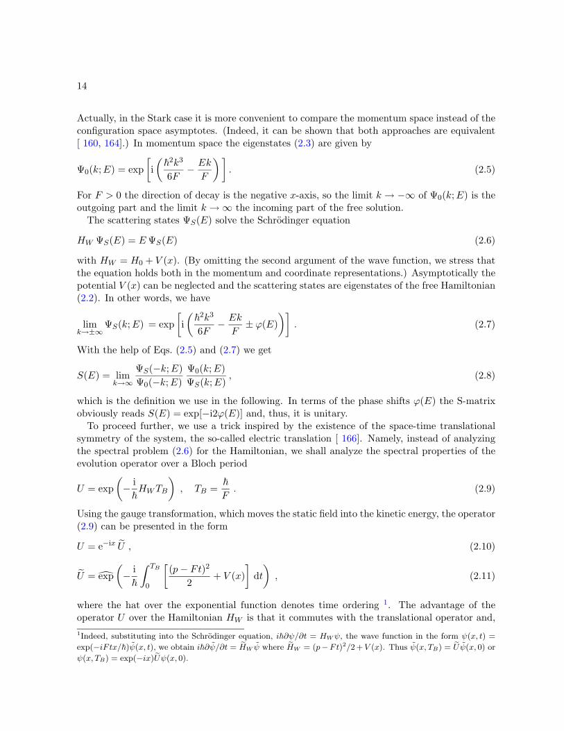
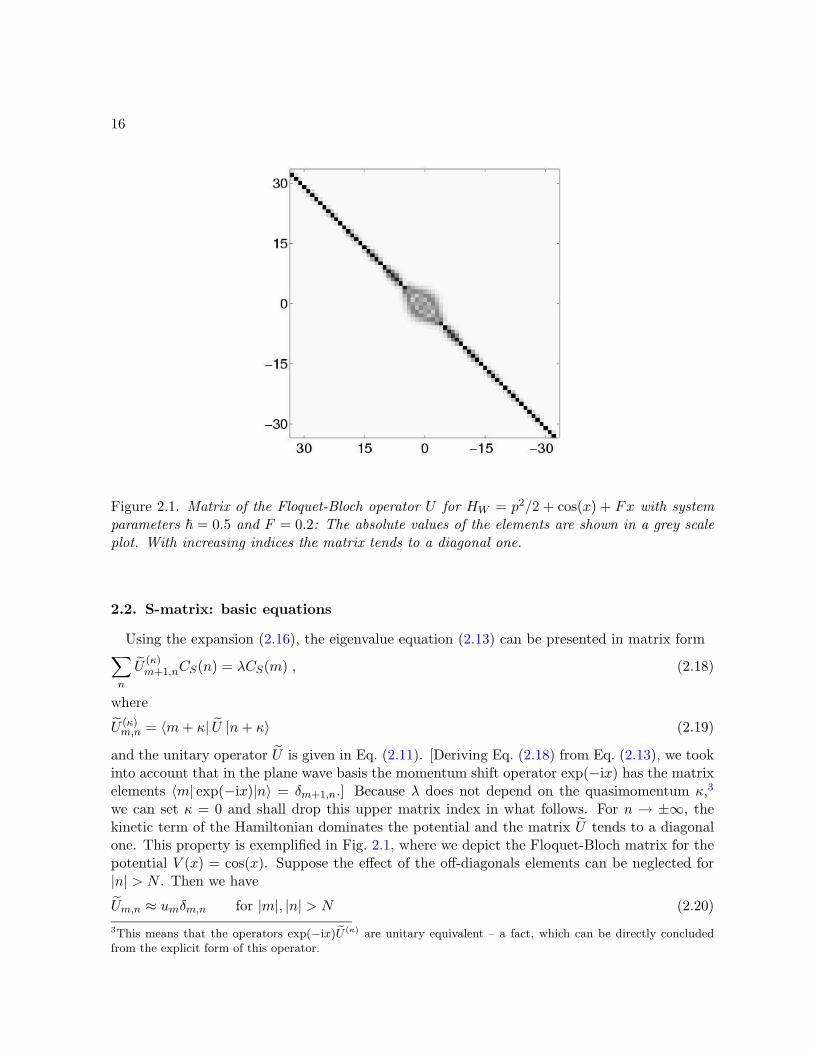
Figure 2.1. Matrix of the Floquet-Bloch operator U for HW = p2/2 + cos(x) + Fx with systemparameters ~ = 0.5 and F = 0.2: The absolute values of the elements are shown in a grey scaleplot. With increasing indices the matrix tends to a diagonal one.

2.2. S-matrix: basic equations

Using the expansion (2.16), the eigenvalue equation (2.13) can be presented in matrix form∑n

U(κ)m+1,nCS(n) = λCS(m) , (2.18)

where

U (κ)m,n = 〈m+ κ| U |n+ κ〉 (2.19)

and the unitary operator U is given in Eq. (2.11). [Deriving Eq. (2.18) from Eq. (2.13), we tookinto account that in the plane wave basis the momentum shift operator exp(−ix) has the matrixelements 〈m| exp(−ix)|n〉 = δm+1,n.] Because λ does not depend on the quasimomentum κ,3

we can set κ = 0 and shall drop this upper matrix index in what follows. For n → ±∞, thekinetic term of the Hamiltonian dominates the potential and the matrix U tends to a diagonalone. This property is exemplified in Fig. 2.1, where we depict the Floquet-Bloch matrix for thepotential V (x) = cos(x). Suppose the effect of the off-diagonals elements can be neglected for|n| > N . Then we have

Um,n ≈ umδm,n for |m|, |n| > N (2.20)3This means that the operators exp(−ix)U (κ) are unitary equivalent – a fact, which can be directly concludedfrom the explicit form of this operator.

17

with

um = exp(− i

2~

∫ TB

0(~m− Ft)2 dt

)= exp

(i~2

6F[(m− 1)3 −m3

]). (2.21)

For the unscattered states Φ0(λ) the formulas (2.20) hold exactly for any m and, given a energyE or λ = exp(−iE/F ), the eigenvalue equation can be solved to yield the discrete version of theAiry function in the momentum representation: C0(m) = exp(i~2m3/6F − iEm/F ). With thehelp of the last equation we have

C0(n)C0(−n)

= exp[i~

2n3

3F− i

2EnF

], (2.22)

which can be now substituted into the S-matrix definition (2.17).We proceed with the scattering states ΦS(λ). Suppose we order the CS with indices increasing

from bottom to top. Then we can decompose the vector CS into three parts,

CS =

C

(+)S

C(0)S

C(−)S

, (2.23)

where C(+)S contains the coefficients for n > N , C(−)

S contains the coefficients for n < −N−1and C(0)

S contains all other coefficients for −N−1 ≤ n ≤ N . The coefficients of C(+)S recursively

depend on the coefficient CS(N), via

CS(m+ 1) = (λ/um+1)CS(m) for m ≥ N . (2.24)

Analogously, the coefficients of C(−)S recursively depend on CS(−N − 1), via

CS(m) = (um+1/λ)CS(m+ 1) for m < −N − 1 . (2.25)

Let us define the matrix W as the matrix U , truncated to the size (2N + 1) × (2N + 1).Furthermore, let BN be the matrix W accomplished by zero column and row vectors:

BN =(~0t 0W ~0

). (2.26)

Then the resulting equation for C(0)S can be written as

(BN − λ11)C(0)S = −uN+1CS(N + 1) e1 , (2.27)

where e1 is a vector of the same length as C(0)S , with the first element equal to one and all others

equal to zero. For a given λ, Eq. (2.27) matches the asymptotes C(+)S and C(−)

S by linking C(+)S ,

via CS(N + 1) and Eq. (2.24), to C(0)S and, via CS(−N − 1) and Eq. (2.25), to C(−)

S . Let us nowintroduce the row vector e1 with all elements equal to zero except the last one, which equals one.Multiplying e1 with C

(0)S yields the last element of the latter one, i.e. CS(−N − 1). Assuming

18

that λ is not an eigenvalue of the matrix BN (this case is treated in the next section) we canmultiply Eq. (2.27) with the inverse of (BN − λ11), which yields

CS(−N − 1)CS(N + 1)

= −uN+1 e1

[BN − e−iE/F 11

]−1e1 . (2.28)

Finally, substituting Eq. (2.22) and Eq. (2.28) into Eq. (2.17), we obtain

S(E) = limN→∞

A(N + 1) e1

[BN − e−iE/F 11

]−1e1 , (2.29)

with a phase factor A(N) = −uNC0(N)/C0(−N), which ensures the convergence of the limitN →∞. The derived Eq. (2.29) defines the scattering matrix of the Wannier-Stark system andis one of our basic equations.

To conclude this section, we note that Eq. (2.29) also provides a direct method to calculatethe so-called Wigner delay time

τ(E) = −i ~∂ lnS(E)

∂E= −2~

∂ϕ(E)∂E

. (2.30)

As shown in Ref. [ 153],

τ(E) = limN→∞

~

F

[ (C

(0)S , C

(0)S

)− 2(N + 1)

]. (2.31)

Thus, one can calculate the delay time from the norm of the C(0)S , which is preferable to (2.30)

from the numerical point of view, because it eliminates an estimation of the derivative. In thesubsequent sections, we shall use the Wigner delay time to analyze the complex spectrum of theWannier-Stark system.

2.3. Calculating the poles of the S-matrix

Let us recall the S-matrix definitions for the Stark system,

S(E) = limk→∞

ΨS(−k;E)ΨS(k;E)

Ψ0(k;E)Ψ0(−k;E)

= limn→∞

CS(−n)CS(n)

C0(n)C0(−n)

. (2.32)

The S-Matrix is an analytic function of the (complex) energy, and we call its isolated poleslocated in the lower half of the complex plane, i.e. those which have an imaginary part less thanzero, resonances. In terms of the asymptotes of the scattering states, resonances correspond toscattering states with purely outgoing asymptotes, i.e. with no incoming wave. (These are theso-called Siegert boundary conditions [ 168].) As one can see directly from (2.22), poles cannotarise from the contributions of the free solutions. In fact, C0(n)/C0(−n) decreases exponentiallyas a function of n for complex energies E = E − iΓ/2. Therefore, poles can arise only from thescattering states CS .

Actually, we already noted the condition for poles in the previous section. In the step fromequation (2.27) to the S-matrix formula (2.29) we needed to invert the matrix (BN − λ11). Wetherefore excluded the case when λ is an eigenvalue of BN . Let us treat it now. If λ is aneigenvalue of BN , the equation defining C(0)

S then reads

(BN − λ11)C(0)S = 0 . (2.33)

19

hbar=1; f=0.07; kappa=0;NN=5; N=2*NN+1; jmax=16; dt=hbar/f/jmax; v=ones(N−1,1);V=0.5*(diag(v,−1)+diag(v,1));p=−hbar*([−NN:NN]’+kappa); U=eye(N);for j=1:jmax,time=dt*(j−0.5);H=diag(0.5*(p−f*time).^2,0)+V;U=expm(−i*dt*H/hbar)*U;end z=zeros(N,1);B=[z’ 0; U z]; d=eig(B);polar(angle(d),abs(d),’*’)

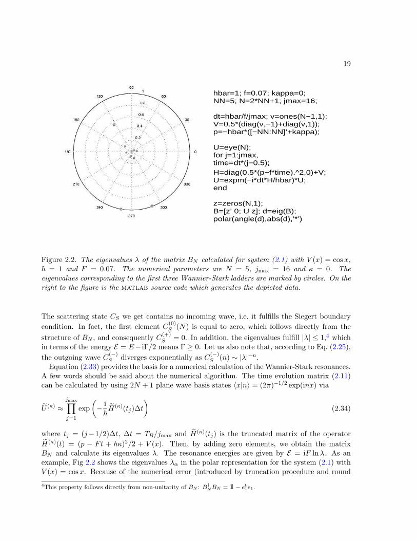
Figure 2.2. The eigenvalues λ of the matrix BN calculated for system (2.1) with V (x) = cosx,~ = 1 and F = 0.07. The numerical parameters are N = 5, jmax = 16 and κ = 0. Theeigenvalues corresponding to the first three Wannier-Stark ladders are marked by circles. On theright to the figure is the matlab source code which generates the depicted data.

The scattering state CS we get contains no incoming wave, i.e. it fulfills the Siegert boundarycondition. In fact, the first element C(0)

S (N) is equal to zero, which follows directly from thestructure of BN , and consequently C(+)

S = 0. In addition, the eigenvalues fulfill |λ| ≤ 1,4 whichin terms of the energy E = E− iΓ/2 means Γ ≥ 0. Let us also note that, according to Eq. (2.25),the outgoing wave C(−)

S diverges exponentially as C(−)S (n) ∼ |λ|−n.

Equation (2.33) provides the basis for a numerical calculation of the Wannier-Stark resonances.A few words should be said about the numerical algorithm. The time evolution matrix (2.11)can be calculated by using 2N + 1 plane wave basis states 〈x|n〉 = (2π)−1/2 exp(inx) via

U (κ) ≈jmax∏j=1

exp(− i~

H(κ)(tj)∆t)

(2.34)

where tj = (j−1/2)∆t, ∆t = TB/jmax and H(κ)(tj) is the truncated matrix of the operatorH(κ)(t) = (p − Ft + ~κ)2/2 + V (x). Then, by adding zero elements, we obtain the matrixBN and calculate its eigenvalues λ. The resonance energies are given by E = iF lnλ. As anexample, Fig 2.2 shows the eigenvalues λα in the polar representation for the system (2.1) withV (x) = cosx. Because of the numerical error (introduced by truncation procedure and round

4This property follows directly from non-unitarity of BN : B†NBN = 11− et1e1.

20

error) not all eigenvalues correspond to the S-matrix poles. The “true” λ can be distinguishedfrom the “false” λ by varying the numerical parameters N , jmax and the quasimomentum κ (werecall that in the case of dc field λ is independent of κ). The true λ are stable against variationof the parameters, but the false λ are not. In Fig 2.2, the stable λ are marked by circles and canbe shown (see next section) to correspond to Wannier-Stark ladders originating from the firstthree Bloch bands. By increasing the accuracy, more true λ (corresponding to higher bands)can be detected.

2.4. Resonance eigenfunctions

According to the results of preceding section, the resonance Bloch-like functions Φα,κ, referredto in what follows as the Wannier-Bloch functions, are given (in the momentum representation)by

Φα,κ(k) =∑n

Cα(n) δ(n+ κ− k) . (2.35)

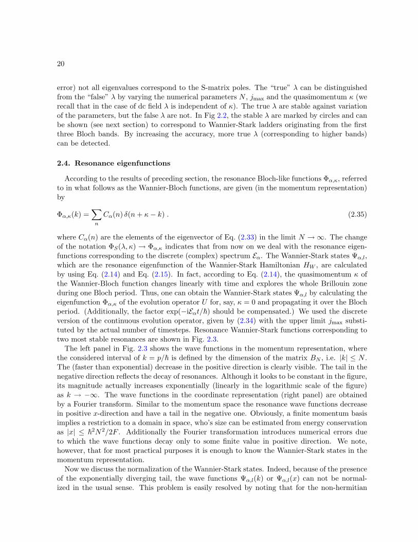
where Cα(n) are the elements of the eigenvector of Eq. (2.33) in the limit N →∞. The changeof the notation ΦS(λ, κ) → Φα,κ indicates that from now on we deal with the resonance eigen-functions corresponding to the discrete (complex) spectrum Eα. The Wannier-Stark states Ψα,l,which are the resonance eigenfunction of the Wannier-Stark Hamiltonian HW , are calculatedby using Eq. (2.14) and Eq. (2.15). In fact, according to Eq. (2.14), the quasimomentum κ ofthe Wannier-Bloch function changes linearly with time and explores the whole Brillouin zoneduring one Bloch period. Thus, one can obtain the Wannier-Stark states Ψα,l by calculating theeigenfunction Φα,κ of the evolution operator U for, say, κ = 0 and propagating it over the Blochperiod. (Additionally, the factor exp(−iEαt/~) should be compensated.) We used the discreteversion of the continuous evolution operator, given by (2.34) with the upper limit jmax substi-tuted by the actual number of timesteps. Resonance Wannier-Stark functions corresponding totwo most stable resonances are shown in Fig. 2.3.

The left panel in Fig. 2.3 shows the wave functions in the momentum representation, wherethe considered interval of k = p/~ is defined by the dimension of the matrix BN , i.e. |k| ≤ N .The (faster than exponential) decrease in the positive direction is clearly visible. The tail in thenegative direction reflects the decay of resonances. Although it looks to be constant in the figure,its magnitude actually increases exponentially (linearly in the logarithmic scale of the figure)as k → −∞. The wave functions in the coordinate representation (right panel) are obtainedby a Fourier transform. Similar to the momentum space the resonance wave functions decreasein positive x-direction and have a tail in the negative one. Obviously, a finite momentum basisimplies a restriction to a domain in space, who’s size can be estimated from energy conservationas |x| ≤ ~

2N2/2F . Additionally the Fourier transformation introduces numerical errors dueto which the wave functions decay only to some finite value in positive direction. We note,however, that for most practical purposes it is enough to know the Wannier-Stark states in themomentum representation.

Now we discuss the normalization of the Wannier-Stark states. Indeed, because of the presenceof the exponentially diverging tail, the wave functions Ψα,l(k) or Ψα,l(x) can not be normal-ized in the usual sense. This problem is easily resolved by noting that for the non-hermitian

21

Figure 2.3. Resonance wave functions of the two most stable resonances of system (2.1) withparameters ~ = 1 and F = 0.07 in momentum and in configuration space. The ground state isplotted as a dashed, the first excited state as a solid line. In the second figure the first excitedstate is shifted by one space period to enhance the visibility.

eigenfunctions (i.e. in the case considered here) the notion of scalar product is modified as∫dxΨ∗α,l(x)Ψα,l(x)→

∫dxΨL

α,l(x)ΨRα,l(x) , (2.36)

where ΨLα,l(x) and ΨR

α,l(x) are the left and right eigenfunctions, respectively. In Fig. 2.3 theright eigenfunctions are depicted. The left eigenfunctions can be calculated in the way describedabove, with the exception that one begins with the left eigenvalue equation C(0)

S (BN − λ11) = 0for the row vector C(0)

S . In the momentum representation, the left function ΨLα,l(k) coincides

with the right one, mirrored relative to k = 0. (Note that in coordinate space, the absolutevalues of both states are identical.) In other words, it corresponds to a scattering state withzero amplitude of the outgoing wave. Since for the right wave function a decay in the positivek-direction is faster than the increase of the left eigenfunction (being inverted, the same is validin the negative k-direction), the scalar product of the left and right eigenfunctions is finite. Inour numerical calculation we typically calculate both functions in the momentum representationand then normalize them according to∫

dkΨLα,l(k)ΨR

β,n(k) = 〈Ψα,l|Ψβ,n〉 = δl,nα,β . (2.37)

(Here and below we use the Dirac notation for the left and right wave functions.) Let us alsorecall the relations

Ψα,l(x) = Ψα,0(x− 2πl) (2.38)

22

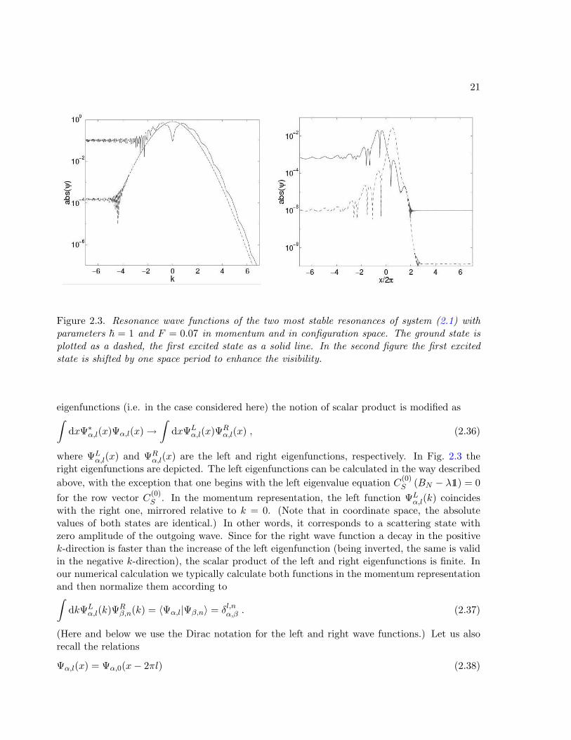
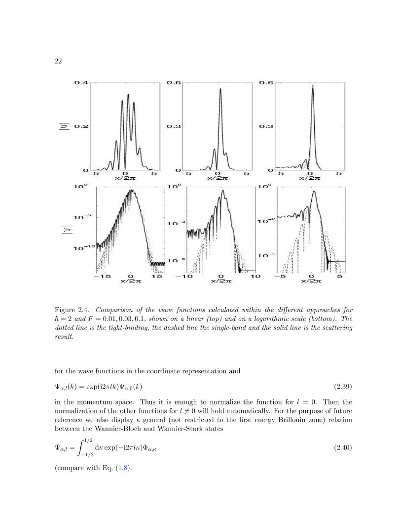
Figure 2.4. Comparison of the wave functions calculated within the different approaches for~ = 2 and F = 0.01, 0.03, 0.1, shown on a linear (top) and on a logarithmic scale (bottom). Thedotted line is the tight-binding, the dashed line the single-band and the solid line is the scatteringresult.

for the wave functions in the coordinate representation and

Ψα,l(k) = exp(i2πlk)Ψα,0(k) (2.39)

in the momentum space. Thus it is enough to normalize the function for l = 0. Then thenormalization of the other functions for l 6= 0 will hold automatically. For the purpose of futurereference we also display a general (not restricted to the first energy Brillouin zone) relationbetween the Wannier-Bloch and Wannier-Stark states

Ψα,l =∫ 1/2

−1/2dκ exp(−i2πlκ)Φα,κ (2.40)

(compare with Eq. (1.8).

23

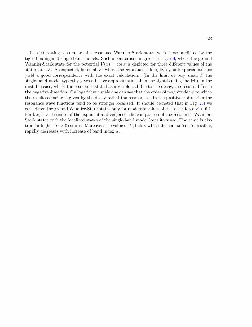
It is interesting to compare the resonance Wannier-Stark states with those predicted by thetight-binding and single-band models. Such a comparison is given in Fig. 2.4, where the groundWannier-Stark state for the potential V (x) = cosx is depicted for three different values of thestatic force F . As expected, for small F , where the resonance is long-lived, both approximationsyield a good correspondence with the exact calculation. (In the limit of very small F thesingle-band model typically gives a better approximation than the tight-binding model.) In theunstable case, where the resonance state has a visible tail due to the decay, the results differ inthe negative direction. On logarithmic scale one can see that the order of magnitude up to whichthe results coincide is given by the decay tail of the resonances. In the positive x-direction theresonance wave functions tend to be stronger localized. It should be noted that in Fig. 2.4 weconsidered the ground Wannier-Stark states only for moderate values of the static force F < 0.1.For larger F , because of the exponential divergence, the comparison of the resonance Wannier-Stark states with the localized states of the single-band model loses its sense. The same is alsotrue for higher (α > 0) states. Moreover, the value of F , below which the comparison is possible,rapidly decreases with increase of band index α.

Chapter 3

Interaction of Wannier-Stark ladders

In this chapter we give a complete description of the dependence of the width Γ of the Wannier-Stark resonances on the parameters of the Wannier-Stark Hamiltonian. In scaled units, theHamiltonian has two independent parameters, the scaled Planck constant ~ and the field strengthF . In our analysis we fix the value of ~ and investigate the width as a function of the fieldstrength. The calculated lifetimes τ = ~/Γ are compared with the experimentally measuredlifetimes of the Wannier-Stark states.

3.1. Resonant tunneling

To get a first glimpse on the subject, we calculate the resonances for the Hamiltonian (2.1)with V (x) = cosx for ~ = 1. For the chosen periodic potential the field-free Hamiltonian hastwo bands with energies well below the potential barrier. For the third band, the energy ε2(κ)can be larger than the potential height. Therefore, with the field switched on, one expects twolong-lived resonance states in each potential well, which are related to the first two bands.

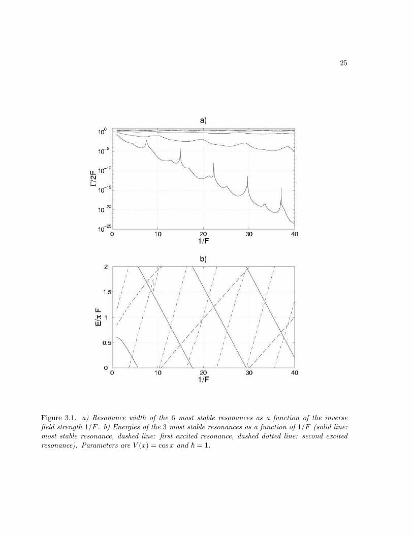
Figure 3.1(a) shows the calculated widths of the six most stable resonances as a functionof the inverse field strength 1/F . The two most stable resonances are clearly separated fromthe other ones. The second excited resonance can still be distinguished from the others, thelifetime of which is similar. Looking at the lifetime of the most stable state, the most strikingphenomenon is the existence of very sharp resonance-like structures, where within a small rangeof F the lifetime can decrease up to six orders of magnitude. In Fig. 3.1(b), we additionallydepict the energies of the three most stable resonances as a function of the inverse field strength.As the Wannier-Stark resonances are arranged in a ladder with spacing ∆E = 2πF , we showonly the first energy Brillouin zone 0 < E/F < 2π. Let us note that the mean slope of thelines in Fig. 3.1(b) defines the absolute position E∗α of the Wannier-Stark resonances in the limitF → 0. As follows from the single band model, these absolute positions can be approximatedby the mean energies εα of the Bloch bands. Depending on the value of E∗α, we can identify aparticular Wannier-Stark resonance either as under- or above-barrier resonance.1

Comparing Fig. 3.1(b) with Fig. 3.1(a), we observe that the decrease in lifetime coincideswith crossings of the energies of the Wannier-Stark resonances. All three possible crossings1This classification holds only in the limit F → 0. In the opposite limit all resonances are obviously above-barrierresonances.

24

25

Figure 3.1. a) Resonance width of the 6 most stable resonances as a function of the inversefield strength 1/F . b) Energies of the 3 most stable resonances as a function of 1/F (solid line:most stable resonance, dashed line: first excited resonance, dashed dotted line: second excitedresonance). Parameters are V (x) = cosx and ~ = 1.

26

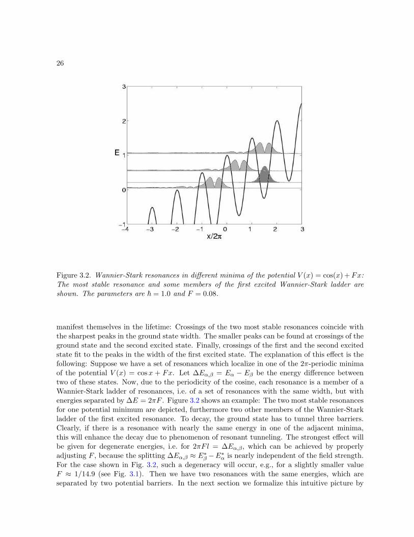
Figure 3.2. Wannier-Stark resonances in different minima of the potential V (x) = cos(x) +Fx:The most stable resonance and some members of the first excited Wannier-Stark ladder areshown. The parameters are ~ = 1.0 and F = 0.08.

manifest themselves in the lifetime: Crossings of the two most stable resonances coincide withthe sharpest peaks in the ground state width. The smaller peaks can be found at crossings of theground state and the second excited state. Finally, crossings of the first and the second excitedstate fit to the peaks in the width of the first excited state. The explanation of this effect is thefollowing: Suppose we have a set of resonances which localize in one of the 2π-periodic minimaof the potential V (x) = cosx + Fx. Let ∆Eα,β = Eα − Eβ be the energy difference betweentwo of these states. Now, due to the periodicity of the cosine, each resonance is a member of aWannier-Stark ladder of resonances, i.e. of a set of resonances with the same width, but withenergies separated by ∆E = 2πF . Figure 3.2 shows an example: The two most stable resonancesfor one potential minimum are depicted, furthermore two other members of the Wannier-Starkladder of the first excited resonance. To decay, the ground state has to tunnel three barriers.Clearly, if there is a resonance with nearly the same energy in one of the adjacent minima,this will enhance the decay due to phenomenon of resonant tunneling. The strongest effect willbe given for degenerate energies, i.e. for 2πF l = ∆Eα,β , which can be achieved by properlyadjusting F , because the splitting ∆Eα,β ≈ E∗β −E∗α is nearly independent of the field strength.For the case shown in Fig. 3.2, such a degeneracy will occur, e.g., for a slightly smaller valueF ≈ 1/14.9 (see Fig. 3.1). Then we have two resonances with the same energies, which areseparated by two potential barriers. In the next section we formalize this intuitive picture by

27

introducing a simple two-ladder model.

3.2. Two interacting Wannier-Stark ladders

It is well known that the interaction between two resonances can be well modeled by a two-state system [ 34, 169, 170, 171]. In this approach the problem reduces to the diagonalization ofa 2×2 matrix, where the diagonal matrix elements correspond to the non-interacting resonances.In our case, however, we have ladders of resonances. This fact can be properly taken into accountby introducing the diagonal matrix in the form [ 155, 160]

U0 = exp(−i

H0

F

), H0 =

(E0 − iΓ0/2 0

0 E1 − iΓ1/2

). (3.1)

It is easy to see that the eigenvalues λ0,1(F ) = exp[−i(E0,1 − iΓ0,1/2]/F ) of U0 correspond tothe relative energies of the Wannier-Stark levels and, thus, the matrix U0 models two crossingladders of resonances.2 Multiplying the matrix U0 by the matrix

Uint = exp[iε(

0 11 0

)]=(

cos ε i sin εi sin ε cos ε

), (3.2)

we introduce an interaction between the ladders. The matrix U0Uint can be diagonalized ana-lytically, which yields

λ± =λ0 + λ1

2cos ε±

[(λ0 + λ1

2

)2

cos2 ε− λ0λ1

]1/2

, λ± = exp(−i

E± − iΓ±/2F

). (3.3)

Based on Eq. (3.3) we distinguish the cases of weak, moderate or strong ladder interaction.The value ε = 0 obviously corresponds to non-interacting ladders. By choosing ε 6= 0 but

ε π/2 we model the case of weakly interacting ladders. In this case the ladders show truecrossing of the real parts and “anticrossing” of the imaginary parts. Thus the interaction affectsonly the stability of the ladders. Indeed, for ε π/2 Eq. (3.3) takes the form

λ± = λ0,1

(1± ε2

2λ0 + λ1

λ1 − λ0

). (3.4)

It follows from the last equation that at the points of crossing (where the phases of λ0 and λ1

coincide) the more stable ladder (let it be the ladder with index 0, i.e. Γ0 < Γ1 or |λ0| > |λ1|)is destabilized (|λ+| < |λ0|) and, vice versa, the less stable ladder becomes more stable (|λ−| >|λ1|). The case of weakly interacting ladders is illustrated by the left column in Fig. 3.3.

By increasing ε above εcr,

sin2 εcr =(|λ0| − |λ1||λ0|+ |λ1|

)2

, (3.5)

the case of moderate interaction, where the true crossing of the real parts E± is substitutedby an anticrossing, is met. As a consequence, the interacting Wannier-Stark ladders exchange2 The resonance energies in Eq. (3.1) actually depend on F but, considering a narrow interval of F , this dependencecan be neglected.

28

Figure 3.3. Illustration to the two-ladder model. Parameters are E0 = 0.3 − i1.1 · 10−2, E1 =0.8− i0.9 · 10−1, and ε = 0.2 (left column), ε = 0.4 (center), and ε = π/2− 0.1 (right column).Upper panels show the energies E±, lower panels the widths Γ±.

their stability index at the point of the avoided crossing (see center column in Fig. 3.3). Themaximally possible interaction is achieved by choosing ε = π/2. Then the eigenvalues of thematrix U0Uint are λ± = ±i(λ0λ1)1/2 which corresponds to the “locked” ladders

E± = (E0 + E1)/2± πF/2 , Γ± = (Γ0 + Γ1)/2 . (3.6)

In other words, the energy levels of one Wannier-Stark ladder are located exactly in the middlebetween the levels of the other ladder (right column in Fig. 3.3).

3.3. Wannier-Stark ladders in optical lattices

In the following two sections we give a comparative analysis of the ladder interaction in opticaland semiconductor superlattices. It will be shown that the character of the interaction can bequalitatively deduced from the Bloch spectrum of the system.

We begin with the optical lattice, which realizes the case of a cosine potential (see Sec. 1.4).A characteristic feature of the cosine potential is an exponential decrease of the band gaps asE → ∞ [see Fig. 1.2(a), for example]. In order to get a satisfactory description of the ladderinteraction for F 6= 0, it is sufficient to consider only the under-barrier resonances and one or

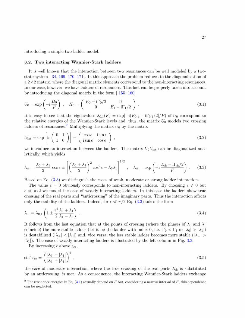
29

Figure 3.4. Widths of the 6 most stable resonances as a function of the inverse field F for~ = 1.0 (solid lines) compared with the fit data (dashed lines).

two above-barrier resonances. In particular, for the parameters of Fig. 3.1 it is enough to “keeptrack” of the resonances belonging to the first three Wannier-Stark ladders. It is also seen inFig. 3.1 that the case of true crossings of the resonances is realized almost exclusively, i.e. theladders are weakly interacting (which is another characteristic property of the cosine potential).The behavior of the resonance widths Γα(F ) at the vicinity of a particular crossing is capturedby Eq. (3.4). Moreover, extending the two-ladder model of the previous section to the threeladder case and assuming the coupling constants in the form

εα = aα exp(−bα/F ) , (3.7)

(which is suggested by the semiclassical arguments of Sec. 1.3) the overall behavior of theresonance width can be perfectly reproduced (see Fig. 3.4). The procedure of adjustment of themodel parameters aα and bα is carefully described in Ref. [ 160].

The lifetime of the Wannier-Stark states (given by τ = ~/Γα) as the function of static forcewas measured in an experiment with cold sodium atoms in a laser field [ 124]. The setting of theexperiment [ 124] yields the accelerated cosine potential (the inertial force takes the role of thestatic field) and an effective Planck constant ~ = 1.671. For this value of the Planck constantone has only one under-barrier resonance, and the two-ladder model of Sec. 3.2 is already agood approximation of the real situation. Figure 3.5 compares the experimental results for thelifetime of the ground Wannier-Stark states with the theoretical results. The axes are adjustedto the experimental parameters. Namely, the field strength in our description is related to the

30

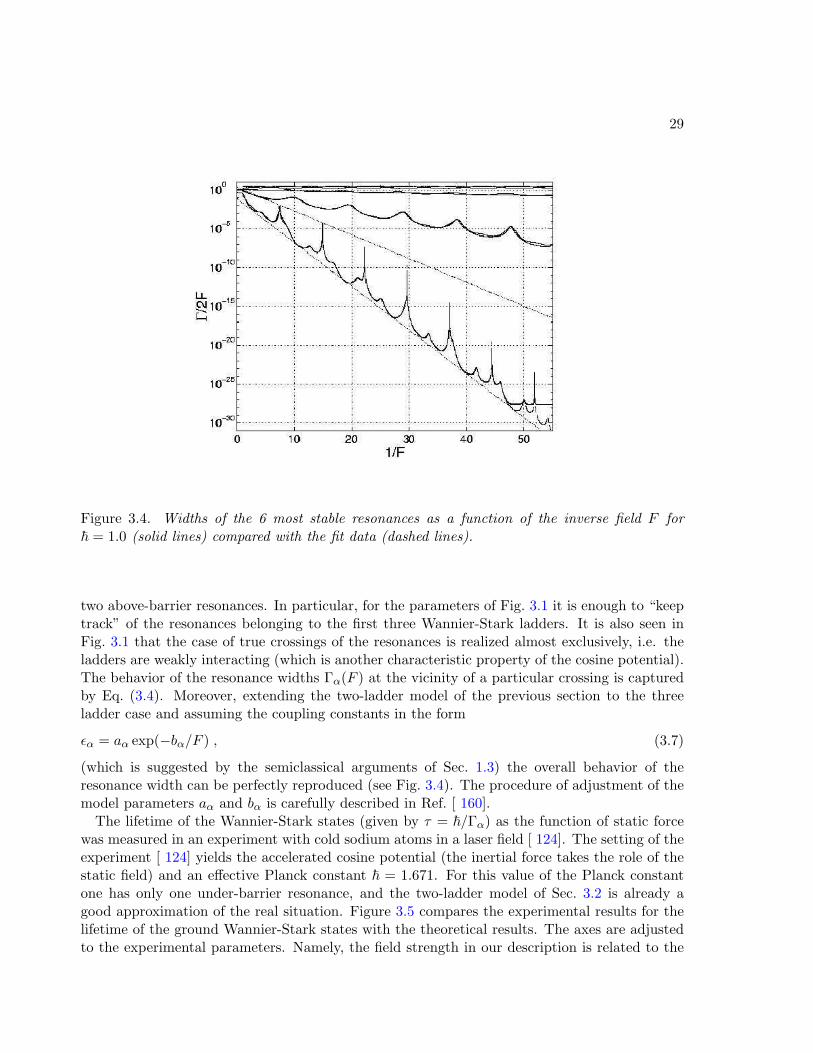
Figure 3.5. Lifetime of the ground Wannier state as a function of the external field. The solidline is the theoretical prediction, the circles are the experimental data of Ref. [ 124]. The insertblows up the interval 4000m/s2 < a < 10000m/s2 considered in the cited experiment.

acceleration in the experiment by the formula F ≈ 0.0383a, where a is measured in km/s2,and the unit of time in our description is approximately 1.34µs. The experimental data followclosely the theoretical curve. (Explicitly, the analytical form of the displayed dependence isgiven by Eq. (3.4) with ε = a exp(−b/F ), a = 1.0, b = 0.254.) In particular we note that thetheory predicts a local minimum of the lifetime at a = 5000m/s2, which corresponds to thecrossing of the ground and the first excited Wannier levels in neighboring wells. Unfortunately,the experimental data do not extend to smaller accelerations, where the theory predicts muchstronger oscillations of the lifetime.

3.4. Wannier-Stark ladders in semiconductor superlattices

We proceed with the semiconductor superlattices. As mentioned in Sec. 1.4, the semiconductorsuperlattices are often modeled by the square-box potential (1.18), where a and b = d − a arethe thickness of the alternating semiconductor layers. For the square-box potential (1.18) thewidth of the band gaps decreases only inversely proportional to the gap’s number. Because ofthis, one is forced to deal with infinite number of interacting Wannier-Stark ladders. However,as was argued in Ref. [ 163], this is actually an over-complication of the real situation. Indeed,the potential (1.18) is only a first approximation for the superlattice potential, which should bea smooth function of x. This fact can be taken into account by smoothing the rectangular step

31

in (1.18) as

V (x) = tanhσ(x+ aπ/2d)− tanhσ(x− aπ/2d)− 1 (3.8)

for example. (Here we use scaled variables, where the potential is 2π-periodic and |V (x)| ≤ 1.)The parameter σ−1 defines the size of the transition region between the semiconductor layersand, in natural units, it cannot be smaller than the atomic distance. The smoothing introducesa cut-off in the energy, above which the gaps between the Bloch bands decrease exponentially.Thus, instead of an infinite number of ladders associated with the above-barrier resonances, wemay consider a finite number of them. The interaction of a large number of ladders originatingfrom the high-energy Bloch bands was studied in some details in Ref. [ 163]. It was found thatthey typically form pairs of locked [in the sense of Eq. (3.6)] ladders which show anticrossingswith each other.

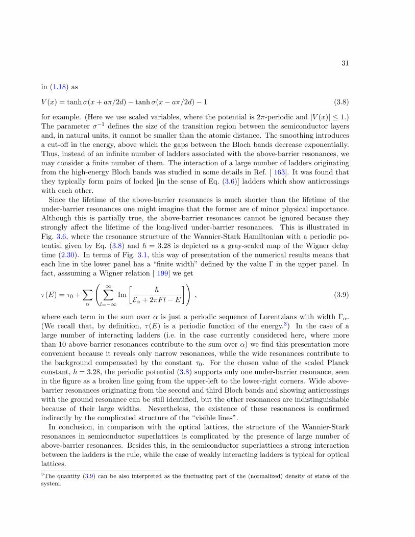
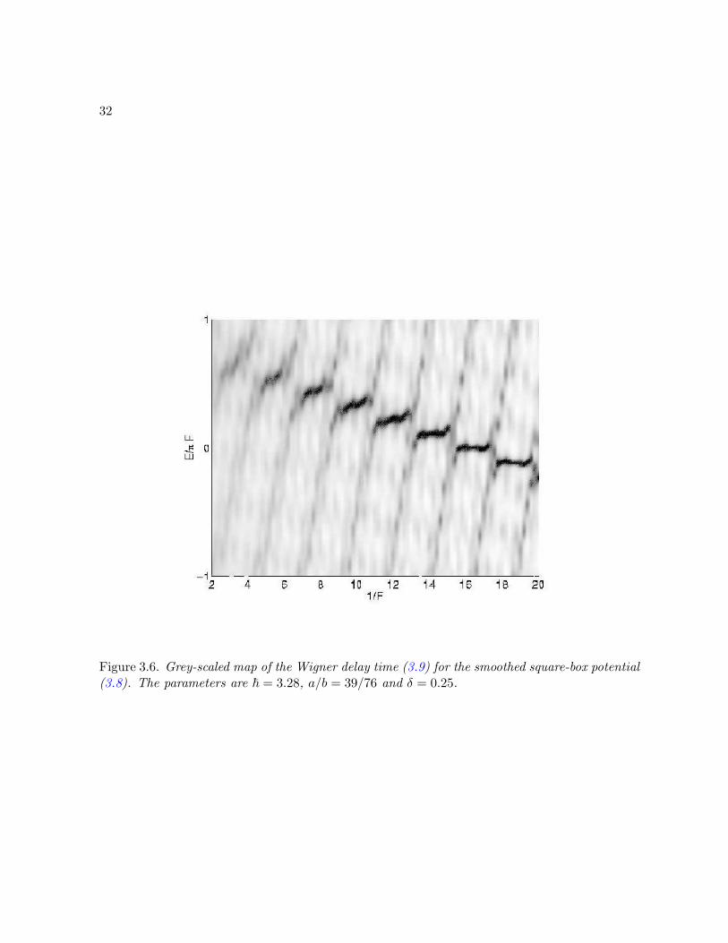
Since the lifetime of the above-barrier resonances is much shorter than the lifetime of theunder-barrier resonances one might imagine that the former are of minor physical importance.Although this is partially true, the above-barrier resonances cannot be ignored because theystrongly affect the lifetime of the long-lived under-barrier resonances. This is illustrated inFig. 3.6, where the resonance structure of the Wannier-Stark Hamiltonian with a periodic po-tential given by Eq. (3.8) and ~ = 3.28 is depicted as a gray-scaled map of the Wigner delaytime (2.30). In terms of Fig. 3.1, this way of presentation of the numerical results means thateach line in the lower panel has a “finite width” defined by the value Γ in the upper panel. Infact, asssuming a Wigner relation [ 199] we get

τ(E) = τ0 +∑α

( ∞∑l=−∞

Im[

~

Eα + 2πF l − E

]), (3.9)

where each term in the sum over α is just a periodic sequence of Lorentzians with width Γα.(We recall that, by definition, τ(E) is a periodic function of the energy.3) In the case of alarge number of interacting ladders (i.e. in the case currently considered here, where morethan 10 above-barrier resonances contribute to the sum over α) we find this presentation moreconvenient because it reveals only narrow resonances, while the wide resonances contribute tothe background compensated by the constant τ0. For the chosen value of the scaled Planckconstant, ~ = 3.28, the periodic potential (3.8) supports only one under-barrier resonance, seenin the figure as a broken line going from the upper-left to the lower-right corners. Wide above-barrier resonances originating from the second and third Bloch bands and showing anticrossingswith the ground resonance can be still identified, but the other resonances are indistinguishablebecause of their large widths. Nevertheless, the existence of these resonances is confirmedindirectly by the complicated structure of the “visible lines”.

In conclusion, in comparison with the optical lattices, the structure of the Wannier-Starkresonances in semiconductor superlattices is complicated by the presence of large number ofabove-barrier resonances. Besides this, in the semiconductor superlattices a strong interactionbetween the ladders is the rule, while the case of weakly interacting ladders is typical for opticallattices.3The quantity (3.9) can be also interpreted as the fluctuating part of the (normalized) density of states of thesystem.

32

Figure 3.6. Grey-scaled map of the Wigner delay time (3.9) for the smoothed square-box potential(3.8). The parameters are ~ = 3.28, a/b = 39/76 and δ = 0.25.

Chapter 4

Spectroscopy of Wannier-Starkladders

In this chapter we discuss the spectroscopy of Wannier-Stark ladders in optical and semiconduc-tor superlattices. We show how the different spectroscopic quantities (measured in a laboratoryexperiment) can be directly calculated by using the formalism of the resonance Wannier-Starkstates.

4.1. Decay spectrum and Fermi’s golden rule

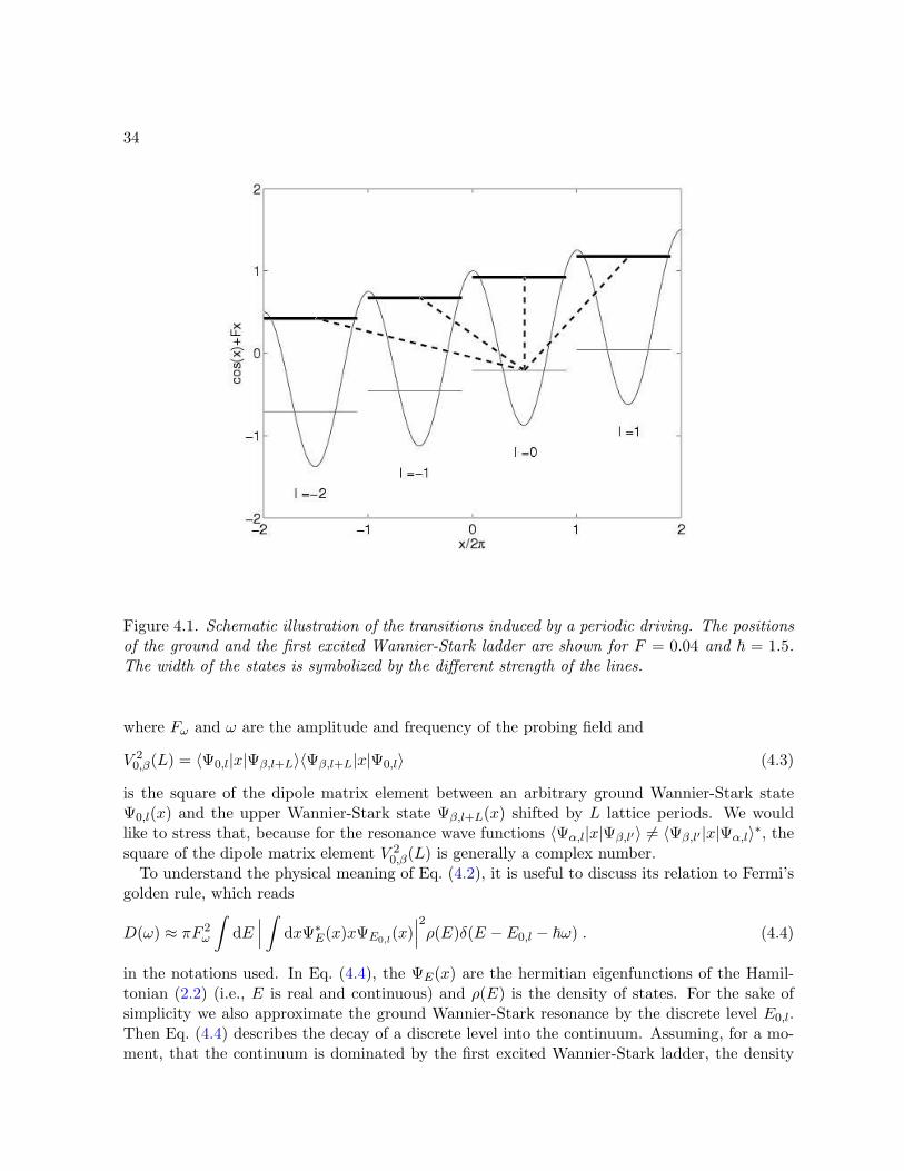
The spectroscopy approach assumes that one probes a quantum system by a weak ac fieldFωx cos(ωt) with tunable frequency ω. In our case, the system consists of different Wannier-Stark ladders of resonances, the two most stable of which are schematically depicted in Fig. 4.1.The driving induces transitions between the ground and the excited states1. Scanning thefrequency ω sequentially activates the different transition paths and the different Wannier statesof the excited ladder are populated. Because the excited states are typically short-lived, theydecay before the driving can transfer the population back to the ground state, i.e. before a Rabioscillation is performed. Then the decay rate of the ground state is determined by the transitionrate D(ω) to the excited Wannier-Stark ladder. The width is written as

Γ0(ω) = Γ0 +D(ω) , (4.1)

where Γ0 takes into account the decay in the absence of driving. In what follows we shall referto the quantity Γ0(ω) as the induced decay rate or the decay spectrum. In Sec. 5 we calculatethe induced decay rate rigorously by using the formalism of quasienergy Wannier-Stark states.It will be shown that the decay spectrum is given by

Γ0(ω) = Γ0 +F 2ω

2

∑β>0

∑L

Im

[V 2

0,β(L)(Eβ,l + 2πFL− E0,l − ~ω)− iΓβ/2

], (4.2)

1Actually, transitions within the same ladder are also induced, but their effect is important only for ω ∼ ωB =2πF/~. Here we shall mainly consider the case ω ωB , where the transitions within the same ladder can beignored.

33

34

Figure 4.1. Schematic illustration of the transitions induced by a periodic driving. The positionsof the ground and the first excited Wannier-Stark ladder are shown for F = 0.04 and ~ = 1.5.The width of the states is symbolized by the different strength of the lines.

where Fω and ω are the amplitude and frequency of the probing field and

V 20,β(L) = 〈Ψ0,l|x|Ψβ,l+L〉〈Ψβ,l+L|x|Ψ0,l〉 (4.3)

is the square of the dipole matrix element between an arbitrary ground Wannier-Stark stateΨ0,l(x) and the upper Wannier-Stark state Ψβ,l+L(x) shifted by L lattice periods. We wouldlike to stress that, because for the resonance wave functions 〈Ψα,l|x|Ψβ,l′〉 6= 〈Ψβ,l′ |x|Ψα,l〉∗, thesquare of the dipole matrix element V 2

0,β(L) is generally a complex number.To understand the physical meaning of Eq. (4.2), it is useful to discuss its relation to Fermi’s

golden rule, which reads

D(ω) ≈ πF 2ω

∫dE∣∣∣ ∫ dxΨ∗E(x)xΨE0,l

(x)∣∣∣2ρ(E)δ(E − E0,l − ~ω) . (4.4)

in the notations used. In Eq. (4.4), the ΨE(x) are the hermitian eigenfunctions of the Hamil-tonian (2.2) (i.e., E is real and continuous) and ρ(E) is the density of states. For the sake ofsimplicity we also approximate the ground Wannier-Stark resonance by the discrete level E0,l.Then Eq. (4.4) describes the decay of a discrete level into the continuum. Assuming, for a mo-ment, that the continuum is dominated by the first excited Wannier-Stark ladder, the density

35

of states ρ(E) is given by a periodic sequence of Lorentzians with width Γ1, i.e.

ρ(E) ≈ 12π

∑L

Γ1

(E − E1,l+L)2 + Γ21/4

. (4.5)

Substituting the last equation into Eq. (4.4) and integrating over E we have

D(ω) ≈ F 2ω

2

∣∣∣ ∫ dxΨ∗E0,l+~ω(x)xΨE0,l

(x)∣∣∣2∑

L

Γ1

(E1,l+L − E0,l − ~ω)2 + Γ21/4

. (4.6)

In the case Γ1 2πF the Lorentzians in the right-hand side of Eq. (4.6) are δ-like functions ofthe argument ~ω = E1,l+ 2πFL−E0,l. Thus the transition matrix element can be moved underthe summation sign, which gives

D(ω) ≈ F 2ω

2

∑β>0

∑L

|V0,β |2(L)Γβ

(Eβ,l + 2πFL− E0,l − ~ω)2 + Γ2β/4

, (4.7)

where

|V0,β |2(L) =∣∣∣ ∫ dxΨ∗Eβ,l+L(x)xΨE0,l

(x)∣∣∣2 (4.8)

(here we again included the possibility of transitions to the higher Wannier ladders, which isindicated by the sum over β). It is seen that that the obtained result coincides with Eq. (4.2) ifthe coefficients |V0,β |2(L) are identified with the squared dipole matrix elements (4.3). Obviously,this holds in the limit F → 0, when the resonance wave functions can be approximated by thelocalized states. For a strong field, however, Eq. (4.7) is a rather poor approximation of thedecay spectrum. In particular, it is unable to predict the non-Lorentzian shape of the lines,which is observed in the laboratory and numerical experiments and which is correctly capturedin Eq. (4.2) by the complex phase of the squared dipole matrix elements V 2

0,β(L).To proceed further, we have to calculate the squared matrix elements (4.3). A rough esti-

mate for V 20,β(L) can be obtained on the basis of Eq. (1.11), which approximates the resonance

Wannier-Stark state by the sum of the localized Wannier states: Ψα,l =∑

m Jm−l(∆α/4πF )ψα,m.The typical experimental settings (see Sec. 4.3) correspond to ∆0/4πF 1 and ∆β/4πF > 1.Then the values of the matrix elements are approximately

V 20,β(L) ≈ |V0,β |2(L) ≈ |〈ψ0,l|x|ψβ,l〉|2J2

L

(∆β

4πF

), (4.9)

which contribute mainly in the region L < ∆β/4πF , the localization length of the excitedWannier-Stark states. The degree of validity of this result is discussed in the next subsection.

4.2. Dipole matrix elements

In this subsection we calculate the dipole matrix elements

Vα,β(l − l′) = 〈Ψα,l|x|Ψβ,l′〉 (4.10)

36

beyond the tight-binding approximation. We shall use Eq. (2.40)

Ψα,l(x) =∫

dκ e−i2πlκΦα,κ(x) , Φα,κ(x) = eiκxχα,κ(x) , χα,κ(x) = χα,κ(x+ 2π) , (4.11)

which relates the Wannier-Stark states Ψα,l(x) to the Wannier-Bloch states Φα,κ(x). As followsfrom the results of Sec. 2, the function χα,κ(x) can be generated from χα,0(x) by propagating itin time

|χα,κ〉 = exp(

iEαt~

)U(t)|χα,0〉 , (4.12)

where U(t) is the continuous version of the operator U defined in Eq. (2.11) and the quasi-momentum κ is related to time t by κ = −Ft/~. Substituting Eq. (4.11) and Eq. (4.12) intoEq. (4.10) we obtain the dipole matrix elements as the Fourier image

Vα,β(l − l′) = 2πl δl,l′

α,β +∫

dκ ei2π(l−l′)κXα,β(κ) (4.13)

of the periodic function

Xα,β(κ) = i 〈χα,κ|∂

∂κχβ,κ〉 =

1F〈χα,κ|

(p+ ~κ)2

2+ V (x) |χβ,κ〉 −

EαFδα,β . (4.14)

The last two equations provide the basis for numerical calculation of the transition matrixelements. We also recall that one actually needs the square of the matrix elements (4.3) butnot the matrix elements themselves (which are defined up to an arbitrary phase). Thus we firstcalculate Vα,β(L) and Vβ,α(L) for L = 0,±1, . . . and then multiply them term by term.

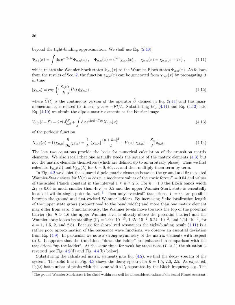
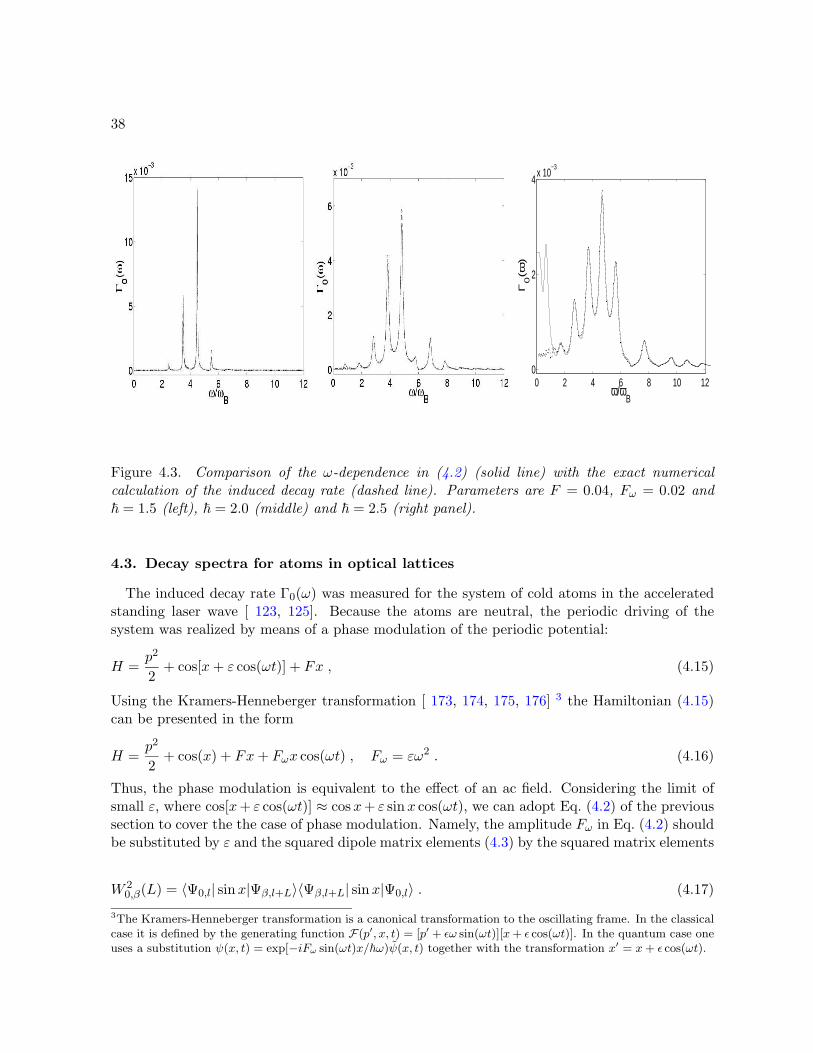
In Fig. 4.2 we depict the squared dipole matrix elements between the ground and first excitedWannier-Stark states for V (x) = cosx, a moderate values of the static force F = 0.04 and valuesof the scaled Planck constant in the interval 1 ≤ ~ ≤ 2.5. For ~ = 1.0 the Bloch bands width∆1 ≈ 0.05 is much smaller than 4πF ≈ 0.5 and the upper Wannier-Stark state is essentiallylocalized within single potential well.2 Then only “vertical” transitions, L = 0, are possiblebetween the ground and first excited Wannier ladders. By increasing ~ the localization lengthof the upper state grows (proportional to the band width) and more than one matrix elementmay differ from zero. Simultaneously, the Wannier levels move towards the top of the potentialbarrier (for ~ > 1.6 the upper Wannier level is already above the potential barrier) and theWannier state looses its stability (Γ1 = 1.90 · 10−15, 1.35 · 10−2, 5.24 · 10−2, and 1.14 · 10−1, for~ = 1, 1.5, 2, and 2.5). Because for short-lived resonances the tight-binding result (1.11) is arather poor approximation of the resonance wave functions, we observe an essential deviationfrom Eq. (4.9). In particular we note a strong asymmetry of the matrix elements with respectto L. It appears that the transitions “down the ladder” are enhanced in comparison with thetransitions “up the ladder”. At the same time, for weak far transitions (L 1) the situation isreversed [see Fig. 4.2(d) and Fig. 4.4(b) below].

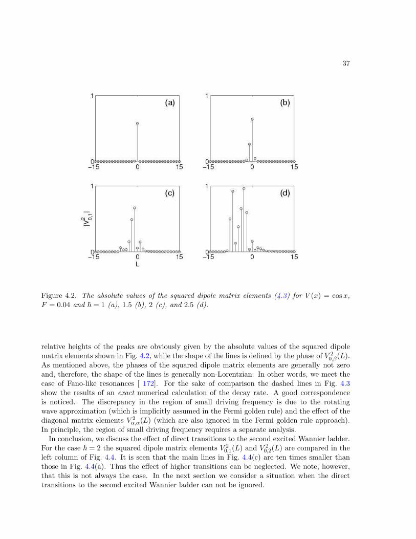
Substituting the calculated matrix elements into Eq. (4.2), we find the decay spectra of thesystem. The solid line in Fig. 4.3 shows the decay spectra for ~ = 1.5, 2.0, 2.5. As expected,Γ0(ω) has number of peaks with the same width Γ1 separated by the Bloch frequency ωB. The2The ground Wannier-Stark state is localized within one well for all considered values of the scaled Planck constant.

37

Figure 4.2. The absolute values of the squared dipole matrix elements (4.3) for V (x) = cosx,F = 0.04 and ~ = 1 (a), 1.5 (b), 2 (c), and 2.5 (d).

relative heights of the peaks are obviously given by the absolute values of the squared dipolematrix elements shown in Fig. 4.2, while the shape of the lines is defined by the phase of V 2

0,β(L).As mentioned above, the phases of the squared dipole matrix elements are generally not zeroand, therefore, the shape of the lines is generally non-Lorentzian. In other words, we meet thecase of Fano-like resonances [ 172]. For the sake of comparison the dashed lines in Fig. 4.3show the results of an exact numerical calculation of the decay rate. A good correspondenceis noticed. The discrepancy in the region of small driving frequency is due to the rotatingwave approximation (which is implicitly assumed in the Fermi golden rule) and the effect of thediagonal matrix elements V 2

α,α(L) (which are also ignored in the Fermi golden rule approach).In principle, the region of small driving frequency requires a separate analysis.

In conclusion, we discuss the effect of direct transitions to the second excited Wannier ladder.For the case ~ = 2 the squared dipole matrix elements V 2

0,1(L) and V 20,2(L) are compared in the

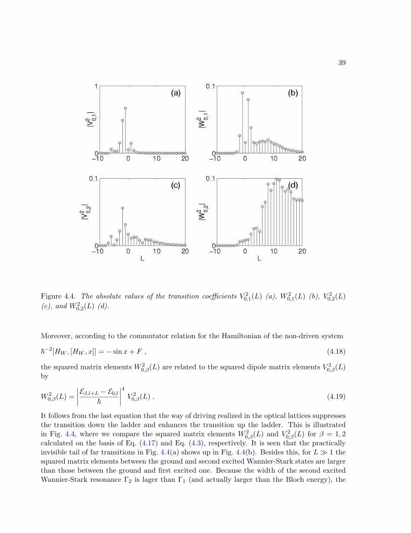
left column of Fig. 4.4. It is seen that the main lines in Fig. 4.4(c) are ten times smaller thanthose in Fig. 4.4(a). Thus the effect of higher transitions can be neglected. We note, however,that this is not always the case. In the next section we consider a situation when the directtransitions to the second excited Wannier ladder can not be ignored.

38

0 2 4 6 8 10 120

2

4x 10

−3

ω/ωB

Γ0(ω

)

Figure 4.3. Comparison of the ω-dependence in (4.2) (solid line) with the exact numericalcalculation of the induced decay rate (dashed line). Parameters are F = 0.04, Fω = 0.02 and~ = 1.5 (left), ~ = 2.0 (middle) and ~ = 2.5 (right panel).

4.3. Decay spectra for atoms in optical lattices

The induced decay rate Γ0(ω) was measured for the system of cold atoms in the acceleratedstanding laser wave [ 123, 125]. Because the atoms are neutral, the periodic driving of thesystem was realized by means of a phase modulation of the periodic potential:

H =p2

2+ cos[x+ ε cos(ωt)] + Fx , (4.15)

Using the Kramers-Henneberger transformation [ 173, 174, 175, 176] 3 the Hamiltonian (4.15)can be presented in the form

H =p2

2+ cos(x) + Fx+ Fωx cos(ωt) , Fω = εω2 . (4.16)

Thus, the phase modulation is equivalent to the effect of an ac field. Considering the limit ofsmall ε, where cos[x+ ε cos(ωt)] ≈ cosx+ ε sinx cos(ωt), we can adopt Eq. (4.2) of the previoussection to cover the the case of phase modulation. Namely, the amplitude Fω in Eq. (4.2) shouldbe substituted by ε and the squared dipole matrix elements (4.3) by the squared matrix elements

W 20,β(L) = 〈Ψ0,l| sinx|Ψβ,l+L〉〈Ψβ,l+L| sinx|Ψ0,l〉 . (4.17)

3The Kramers-Henneberger transformation is a canonical transformation to the oscillating frame. In the classicalcase it is defined by the generating function F(p′, x, t) = [p′ + εω sin(ωt)][x+ ε cos(ωt)]. In the quantum case oneuses a substitution ψ(x, t) = exp[−iFω sin(ωt)x/~ω)ψ(x, t) together with the transformation x′ = x+ ε cos(ωt).

39

Figure 4.4. The absolute values of the transition coefficients V 20,1(L) (a), W 2

0,1(L) (b), V 20,2(L)

(c), and W 20,2(L) (d).

Moreover, according to the commutator relation for the Hamiltonian of the non-driven system

~−2[HW , [HW , x]] = − sinx+ F , (4.18)

the squared matrix elements W 20,β(L) are related to the squared dipole matrix elements V 2

0,β(L)by

W 20,β(L) =

∣∣∣∣Eβ,l+L − E0,l

~

∣∣∣∣4 V 20,β(L) . (4.19)

It follows from the last equation that the way of driving realized in the optical lattices suppressesthe transition down the ladder and enhances the transition up the ladder. This is illustratedin Fig. 4.4, where we compare the squared matrix elements W 2

0,β(L) and V 20,β(L) for β = 1, 2

calculated on the basis of Eq. (4.17) and Eq. (4.3), respectively. It is seen that the practicallyinvisible tail of far transitions in Fig. 4.4(a) shows up in Fig. 4.4(b). Besides this, for L 1 thesquared matrix elements between the ground and second excited Wannier-Stark states are largerthan those between the ground and first excited one. Because the width of the second excitedWannier-Stark resonance Γ2 is lager than Γ1 (and actually larger than the Bloch energy), the

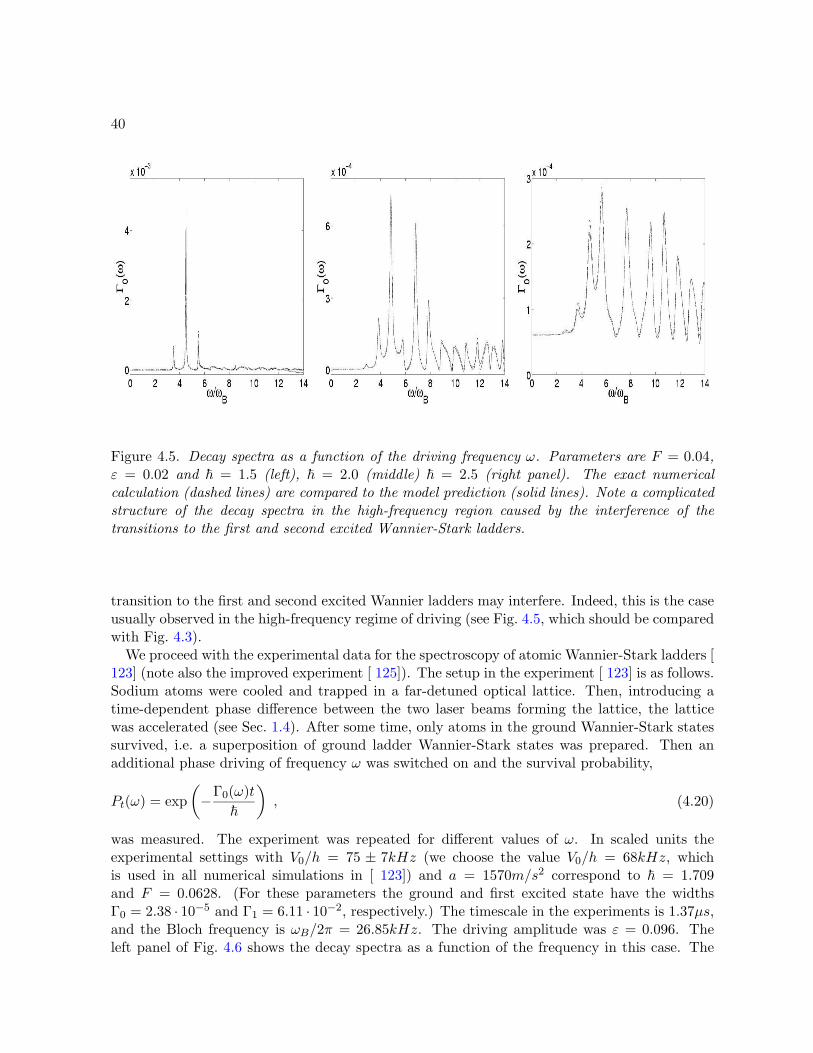
40

Figure 4.5. Decay spectra as a function of the driving frequency ω. Parameters are F = 0.04,ε = 0.02 and ~ = 1.5 (left), ~ = 2.0 (middle) ~ = 2.5 (right panel). The exact numericalcalculation (dashed lines) are compared to the model prediction (solid lines). Note a complicatedstructure of the decay spectra in the high-frequency region caused by the interference of thetransitions to the first and second excited Wannier-Stark ladders.

transition to the first and second excited Wannier ladders may interfere. Indeed, this is the caseusually observed in the high-frequency regime of driving (see Fig. 4.5, which should be comparedwith Fig. 4.3).

We proceed with the experimental data for the spectroscopy of atomic Wannier-Stark ladders [123] (note also the improved experiment [ 125]). The setup in the experiment [ 123] is as follows.Sodium atoms were cooled and trapped in a far-detuned optical lattice. Then, introducing atime-dependent phase difference between the two laser beams forming the lattice, the latticewas accelerated (see Sec. 1.4). After some time, only atoms in the ground Wannier-Stark statessurvived, i.e. a superposition of ground ladder Wannier-Stark states was prepared. Then anadditional phase driving of frequency ω was switched on and the survival probability,

Pt(ω) = exp(−Γ0(ω)t

~

), (4.20)

was measured. The experiment was repeated for different values of ω. In scaled units theexperimental settings with V0/h = 75 ± 7kHz (we choose the value V0/h = 68kHz, whichis used in all numerical simulations in [ 123]) and a = 1570m/s2 correspond to ~ = 1.709and F = 0.0628. (For these parameters the ground and first excited state have the widthsΓ0 = 2.38 · 10−5 and Γ1 = 6.11 · 10−2, respectively.) The timescale in the experiments is 1.37µs,and the Bloch frequency is ωB/2π = 26.85kHz. The driving amplitude was ε = 0.096. Theleft panel of Fig. 4.6 shows the decay spectra as a function of the frequency in this case. The

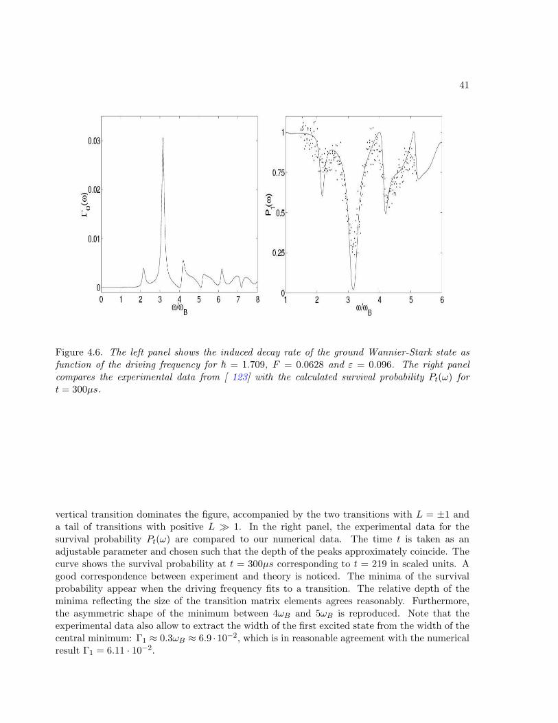
41

Figure 4.6. The left panel shows the induced decay rate of the ground Wannier-Stark state asfunction of the driving frequency for ~ = 1.709, F = 0.0628 and ε = 0.096. The right panelcompares the experimental data from [ 123] with the calculated survival probability Pt(ω) fort = 300µs.

vertical transition dominates the figure, accompanied by the two transitions with L = ±1 anda tail of transitions with positive L 1. In the right panel, the experimental data for thesurvival probability Pt(ω) are compared to our numerical data. The time t is taken as anadjustable parameter and chosen such that the depth of the peaks approximately coincide. Thecurve shows the survival probability at t = 300µs corresponding to t = 219 in scaled units. Agood correspondence between experiment and theory is noticed. The minima of the survivalprobability appear when the driving frequency fits to a transition. The relative depth of theminima reflecting the size of the transition matrix elements agrees reasonably. Furthermore,the asymmetric shape of the minimum between 4ωB and 5ωB is reproduced. Note that theexperimental data also allow to extract the width of the first excited state from the width of thecentral minimum: Γ1 ≈ 0.3ωB ≈ 6.9 ·10−2, which is in reasonable agreement with the numericalresult Γ1 = 6.11 · 10−2.

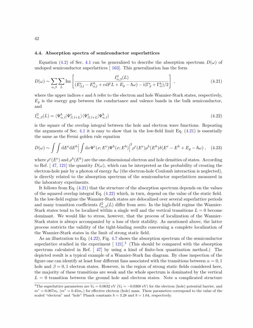
42

4.4. Absorption spectra of semiconductor superlattices

Equation (4.2) of Sec. 4.1 can be generalized to describe the absorption spectrum D(ω) ofundoped semiconductor superlattices [ 163]. This generalization has the form

D(ω) ∼∑α,β

∑L

Im

[I2α,β(L)

(Eeβ,l − Ehα,l + edFL+ Eg − ~ω)− i(Γeβ + Γhα)/2

], (4.21)

where the upper indices e and h refer to the electron and hole Wannier-Stark states, respectively,Eg is the energy gap between the conductance and valence bands in the bulk semiconductor,and

I2α, β(L) = 〈Ψh

α, l|Ψeβ, l+L〉〈Ψe

β, l+L|Ψhα, l〉 (4.22)

is the square of the overlap integral between the hole and electron wave functions. Repeatingthe arguments of Sec. 4.1 it is easy to show that in the low-field limit Eq. (4.21) is essentiallythe same as the Fermi golden rule equation

D(ω) ∼∫ ∫

dEedEh∣∣∣ ∫ dxΨe(x;Ee)Ψh(x;Eh)

∣∣∣2ρe(Ee)ρh(Eh)δ(Ee − Eh + Eg − ~ω) , (4.23)

where ρe(Ee) and ρh(Eh) are the one-dimensional electron and hole densities of states. Accordingto Ref. [ 47, 121] the quantity D(ω), which can be interpreted as the probability of creating theelectron-hole pair by a photon of energy ~ω (the electron-hole Coulomb interaction is neglected),is directly related to the absorption spectrum of the semiconductor superlattices measured inthe laboratory experiments.

It follows from Eq. (4.21) that the structure of the absorption spectrum depends on the valuesof the squared overlap integral Eq. (4.22) which, in turn, depend on the value of the static field.In the low-field regime the Wannier-Stark states are delocalized over several superlattice periodsand many transition coefficients I2

α, β(L) differ from zero. In the high-field regime the Wannier-Stark states tend to be localized within a single well and the vertical transitions L = 0 becomedominant. We would like to stress, however, that the process of localization of the Wannier-Stark states is always accompanied by a loss of their stability. As mentioned above, the latterprocess restricts the validity of the tight-binding results concerning a complete localization ofthe Wannier-Stark states in the limit of strong static field.

As an illustration to Eq. (4.22), Fig. 4.7 shows the absorption spectrum of the semiconductorsuperlattice studied in the experiment [ 121].4 (This should be compared with the absorptionspectrum calculated in Ref. [ 47] by using a kind of finite-box quantization method.) Thedepicted result is a typical example of a Wannier-Stark fan diagram. By close inspection of thefigure one can identify at least four different fans associated with the transitions between α = 0, 1hole and β = 0, 1 electron states. However, in the region of strong static fields considered here,the majority of these transitions are weak and the whole spectrum is dominated by the verticalL = 0 transition between the ground hole and electron states. Note a complicated structure4The superlattice parameters are V0 = 0.0632 eV (V0 = −0.0368 eV) for the electron (hole) potential barrier, andm∗ = 0.067me (m∗ = 0.45me) for effective electron (hole) mass. These parameters correspond to the value of thescaled “electron” and “hole” Planck constants ~ = 3.28 and ~ = 1.64, respectively.

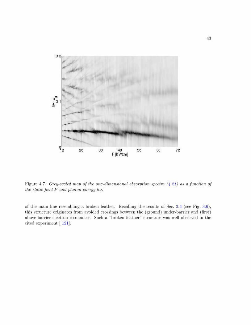
43

Figure 4.7. Grey-scaled map of the one-dimensional absorption spectra (4.21) as a function ofthe static field F and photon energy hν.

of the main line resembling a broken feather. Recalling the results of Sec. 3.4 (see Fig. 3.6),this structure originates from avoided crossings between the (ground) under-barrier and (first)above-barrier electron resonances. Such a “broken feather” structure was well observed in thecited experiment [ 121].

Chapter 5

Quasienergy Wannier-Stark states

In the following chapters we investigate Wannier-Stark ladders in combined ac and dc fields.Then the Hamiltonian of the system is

H =p2

2+ V (x) + Fx+ Fωx cos(ωt) , (5.1)

or, as described in Sec. 4.3, equivalently given by

H =p2

2+ V [x+ ε cos(ωt)] + Fx , ε = Fω/ω

2 . (5.2)

Depending on the particular analytical approach we shall use either of these two forms. Let usalso note that the Hamiltonian (5.2) can be generalized to include the case of arbitrary space-and time-periodic potential V (x, t) = V (x+ 2π, t) = V (x, t+ Tω).

5.1. Single-band quasienergy spectrum

For time-dependent potentials the period of the potential sets an additional time scale. Inorder to define a Floquet-Bloch operator with properties similar to the time-independent case, wehave the restriction that the period Tω of the potential and the Bloch time TB are commensurate,i.e.

pTω = qTB ≡ T . (5.3)

In this case the Floquet operator U(T ) over the common period T can be presented as

U(T ) = e−iqx U(T ) , U(T ) = exp(− i~

∫ T

0dt[

(p− Ft)2

2+ V (x, t)

]), (5.4)

(compare with Eqs. (2.10)–(2.11)). Consequently the eigenstates of U(T ),

U(T ) Φ(x;λ, κ) = λΦ(x;λ, κ) , λ = exp(−iET/~) , (5.5)

can be chosen to be the Bloch-like states [ 177, 178], i.e. Φ(x+ 2π;λ, κ) = ei2πκΦ(x;λ, κ). Dueto the time-periodicity of the potential, V (x, t+ Tω) = V (x, t), we have the relation

U(T ) = U(Tω)p =[exp(−ix q/p) U(Tω)

]p. (5.6)

44

45

As a direct consequence of this relation, the states Φ(x;λ, κ) with the quasimomentum κ− r/p(r = 0, 1, . . . , p − 1) are Floquet states with the same quasienergy. In terms of the operatorU (κ)(T ) = exp(−iκx)U(T ) exp(iκx) this means that the operators U (κ)(T ) are unitarily equiv-alent for these values of the quasimomentum.1 Therefore, the Brillouin zone of the Floquetoperator U(T ) is p-fold degenerate. In the next section we introduce the resonance Wannier-Bloch functions Φα,κ(x) which satisfy the eigenvalue equation (5.5) with the Siegert (i.e. purelyoutgoing wave) boundary condition and correspond to the complex energy Eα(κ). Then the p-fold degeneracy of the Brillouin zone just means that the dispersion relation Eα(κ) is a periodicfunction of the quasimomentum with period given by p.

It should be noted that the Wannier-Bloch functions Φ(x;λ, κ) (hermitian boundary condition)or Φα,κ(x) (Siegert boundary condition) are not the quasienergy functions of the system becausethe latter, by definition, are the eigenfunctions of the evolution operator U(Tω) over the periodof the driving force. However, the quasienergy functions can be expressed in terms of theWannier-Bloch functions as

Ψ(n)α,κ(x) =

1p

p−1∑r=0

exp[−i

2πnpr

]Φα,κ+r/p(x) . (5.7)

Equation (5.7) is the discrete analogue of the relation (2.40) between the Wannier-Bloch andWannier-Stark states in the case of pure dc field. Since the evolution operator U(Tω) commuteswith the translational operator over p lattice periods, the quasienergy states Ψ(n)

α,κ(x) are theeigenfunctions of this shift operator. In particular, as easily deduced from Eq. (5.7), in the limitε → 0 the function Ψ(n)

α,κ(x) is a linear combination of every p-th state of the Wannier-Starkladder (and altogether there are p different subladders). Thus, as well as the Wannier-Blochstates Φα,κ(x), the eigenstates of U(Tω) are extended states. Note that the Brillouin zone isreduced now by a factor p, i.e the quasimomentum is restricted to −1/2p ≤ κ ≤ 1/2p. Onthe other hand, as Tω = T/p, the energy Brillouin zone is enlarged by this factor, i.e. thequasienergies take values in the interval 0 ≤ Re E ≤ ~ω. Thus, if Eα(κ) is the complex band ofthe Floquet operator (5.4), the complex quasienergies corresponding to the quasienergy states(5.7) are

E(n)α (κ) = Eα(κ) + ~ω

n

p, ~ω = 2πF

p

q. (5.8)

In the remainder of this section we discuss the dispersion relation Eα(κ) for the quasienergybands on the basis of the single-band model. It is understood, however, that the single-bandapproach can describe at its best only the real part E = ReE of the spectrum.

In the single band analysis [ 54], it is convenient to work in the representation (5.1). Assumingthat the two timescales are commensurate, the Houston functions (1.13) can be generalized tothe Wannier-Bloch functions, which yields the following result for the quasienergy spectrum

Eα(κ) =1T

∫ T

0εα(κ(t) ) dt , κ(t) = κ− Ft

~

− Fω~ω

sin(ωt) , (5.9)

In this equation, as before, εα(κ) is the Bloch spectrum of the field-free Hamiltonian H0 =p2/2 + V (x) and κ(t) is the solution of the classical equation of motion for the quasimomentum1We recall that in the case of pure dc field the operators U (κ)(TB) are unitarily equivalent for arbitrary κ.

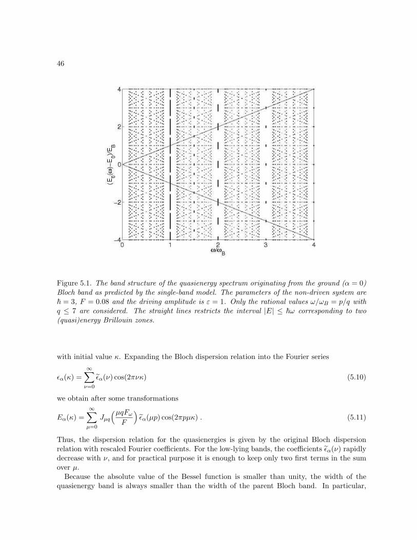
46

Figure 5.1. The band structure of the quasienergy spectrum originating from the ground (α = 0)Bloch band as predicted by the single-band model. The parameters of the non-driven system are~ = 3, F = 0.08 and the driving amplitude is ε = 1. Only the rational values ω/ωB = p/q withq ≤ 7 are considered. The straight lines restricts the interval |E| ≤ ~ω corresponding to two(quasi)energy Brillouin zones.

with initial value κ. Expanding the Bloch dispersion relation into the Fourier series

εα(κ) =∞∑ν=0

εα(ν) cos(2πνκ) (5.10)

we obtain after some transformations

Eα(κ) =∞∑µ=0

Jµq

(µqFωF

)εα(µp) cos(2πpµκ) . (5.11)

Thus, the dispersion relation for the quasienergies is given by the original Bloch dispersionrelation with rescaled Fourier coefficients. For the low-lying bands, the coefficients εα(ν) rapidlydecrease with ν, and for practical purpose it is enough to keep only two first terms in the sumover µ.

Because the absolute value of the Bessel function is smaller than unity, the width of thequasienergy band is always smaller than the width of the parent Bloch band. In particular,

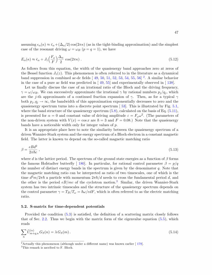
47

assuming εα(κ) ≈ εα+(∆α/2) cos(2πκ) (as in the tight-binding approximation) and the simplestcase of the resonant driving ω = ωB (p = q = 1), we have

Eα(κ) ≈ εα + J1

(FωF

)∆α

2cos(2πκ) . (5.12)

As follows from this equation, the width of the quasienergy band approaches zero at zeros ofthe Bessel function J1(z). This phenomenon is often referred to in the literature as a dynamicalband suppression in combined ac-dc fields [ 49, 50, 51, 52, 53, 54, 55, 56] 2. A similar behaviorin the case of a pure ac field was predicted in [ 49, 55] and experimentally observed in [ 138].

Let us finally discuss the case of an irrational ratio of the Bloch and the driving frequency,γ = ω/ωB. We can successively approximate the irrational γ by rational numbers pj/qj , whichare the j-th approximants of a continued fraction expansion of γ. Then, as for a typical γboth pj , qj →∞, the bandwidth of this approximation exponentially decreases to zero and thequasienergy spectrum turns into a discrete point spectrum [ 53]. This is illustrated by Fig. 5.1,where the band structure of the quasienergy spectrum (5.8), calculated on the basis of Eq. (5.11),is presented for α = 0 and constant value of driving amplitude ε = Fωω

2. (The parameters ofthe non-driven system with V (x) = cosx are ~ = 3 and F = 0.08.) Note that the quasienergybands have a noticeable width only for integer values of p.

It is an appropriate place here to note the similarity between the quasienergy spectrum of adriven Wannier-Stark system and the energy spectrum of a Bloch electron in a constant magneticfield. The latter is known to depend on the so-called magnetic matching ratio

β =eBd2

2π~c, (5.13)

where d is the lattice period. The spectrum of the ground state energies as a function of β formsthe famous Hofstadter butterfly [ 180]. In particular, for rational control parameter β = p/qthe number of distinct energy bands in the spectrum is given by the denominator q. Note thatthe magnetic matching ratio can be interpreted as ratio of two timescales, one of which is thetime d2m/2π~ a particle with momentum 2π~/d needs to cross the fundamental period d, andthe other is the period eB/mc of the cyclotron motion.3 Similar, the driven Wannier-Starksystem has two intrinsic timescales and the structure of the quasienergy spectrum depends onthe control parameter γ = TB/Tω = ~ω/edF , which is often referred to as the electric matchingratio.

5.2. S-matrix for time-dependent potentials

Provided the condition (5.3) is satisfied, the definition of a scattering matrix closely followsthat of Sec. 2.2. Thus we begin with the matrix form of the eigenvalue equation (5.5), whichreads∑n

U(κ)m+q,nGS(n) = λGS(m) . (5.14)

2Actually this phenomenon (although under a different name) was known earlier [ 179].3This remark is ascribed to F. Bloch.

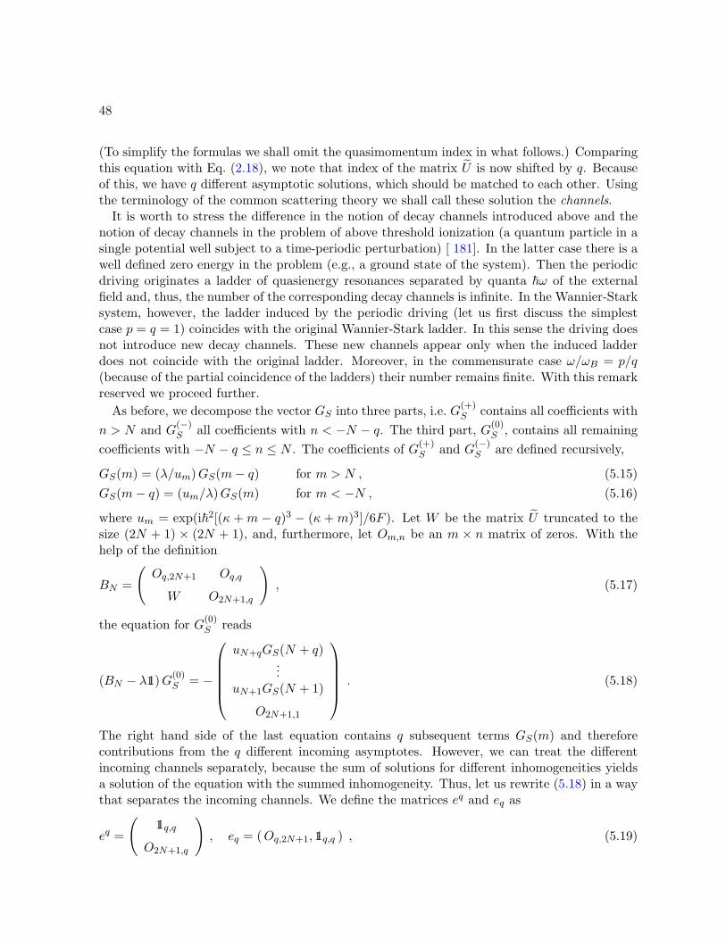
48

(To simplify the formulas we shall omit the quasimomentum index in what follows.) Comparingthis equation with Eq. (2.18), we note that index of the matrix U is now shifted by q. Becauseof this, we have q different asymptotic solutions, which should be matched to each other. Usingthe terminology of the common scattering theory we shall call these solution the channels.

It is worth to stress the difference in the notion of decay channels introduced above and thenotion of decay channels in the problem of above threshold ionization (a quantum particle in asingle potential well subject to a time-periodic perturbation) [ 181]. In the latter case there is awell defined zero energy in the problem (e.g., a ground state of the system). Then the periodicdriving originates a ladder of quasienergy resonances separated by quanta ~ω of the externalfield and, thus, the number of the corresponding decay channels is infinite. In the Wannier-Starksystem, however, the ladder induced by the periodic driving (let us first discuss the simplestcase p = q = 1) coincides with the original Wannier-Stark ladder. In this sense the driving doesnot introduce new decay channels. These new channels appear only when the induced ladderdoes not coincide with the original ladder. Moreover, in the commensurate case ω/ωB = p/q(because of the partial coincidence of the ladders) their number remains finite. With this remarkreserved we proceed further.

As before, we decompose the vector GS into three parts, i.e. G(+)S contains all coefficients with

n > N and G(−)S all coefficients with n < −N − q. The third part, G(0)

S , contains all remainingcoefficients with −N − q ≤ n ≤ N . The coefficients of G(+)

S and G(−)S are defined recursively,

GS(m) = (λ/um)GS(m− q) for m > N , (5.15)GS(m− q) = (um/λ)GS(m) for m < −N , (5.16)

where um = exp(i~2[(κ + m − q)3 − (κ + m)3]/6F ). Let W be the matrix U truncated to thesize (2N + 1) × (2N + 1), and, furthermore, let Om,n be an m × n matrix of zeros. With thehelp of the definition

BN =

(Oq,2N+1 Oq,q

W O2N+1,q

), (5.17)

the equation for G(0)S reads

(BN − λ11)G(0)S = −

uN+qGS(N + q)

...uN+1GS(N + 1)

O2N+1,1

. (5.18)

The right hand side of the last equation contains q subsequent terms GS(m) and thereforecontributions from the q different incoming asymptotes. However, we can treat the differentincoming channels separately, because the sum of solutions for different inhomogeneities yieldsa solution of the equation with the summed inhomogeneity. Thus, let us rewrite (5.18) in a waythat separates the incoming channels. We define the matrices eq and eq as

eq =

(11q,q

O2N+1,q

), eq = (Oq,2N+1, 11q,q ) , (5.19)

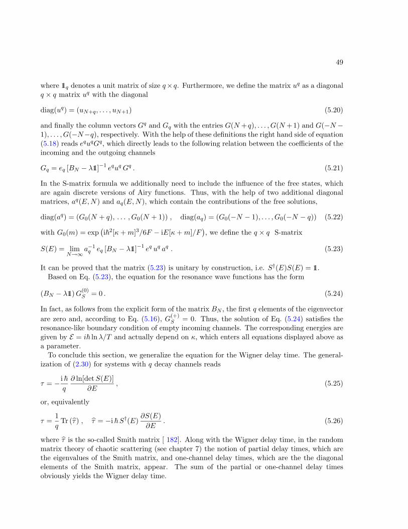
49

where 11q denotes a unit matrix of size q×q. Furthermore, we define the matrix uq as a diagonalq × q matrix uq with the diagonal

diag(uq) = (uN+q, . . . , uN+1) (5.20)

and finally the column vectors Gq and Gq with the entries G(N + q), . . . , G(N +1) and G(−N −1), . . . , G(−N−q), respectively. With the help of these definitions the right hand side of equation(5.18) reads equqGq, which directly leads to the following relation between the coefficients of theincoming and the outgoing channels

Gq = eq [BN − λ11]−1 equq Gq . (5.21)

In the S-matrix formula we additionally need to include the influence of the free states, whichare again discrete versions of Airy functions. Thus, with the help of two additional diagonalmatrices, aq(E,N) and aq(E,N), which contain the contributions of the free solutions,

diag(aq) = (G0(N + q), . . . , G0(N + 1)) , diag(aq) = (G0(−N − 1), . . . , G0(−N − q)) (5.22)

with G0(m) = exp(i~2[κ+m]3/6F − iE[κ+m]/F

), we define the q × q S-matrix

S(E) = limN→∞

a−1q eq [BN − λ11]−1 eq uq aq . (5.23)

It can be proved that the matrix (5.23) is unitary by construction, i.e. S†(E)S(E) = 11.Based on Eq. (5.23), the equation for the resonance wave functions has the form

(BN − λ11)G(0)S = 0 . (5.24)

In fact, as follows from the explicit form of the matrix BN , the first q elements of the eigenvectorare zero and, according to Eq. (5.16), G(+)

S = 0. Thus, the solution of Eq. (5.24) satisfies theresonance-like boundary condition of empty incoming channels. The corresponding energies aregiven by E = i~ lnλ/T and actually depend on κ, which enters all equations displayed above asa parameter.

To conclude this section, we generalize the equation for the Wigner delay time. The general-ization of (2.30) for systems with q decay channels reads

τ = − i ~q

∂ ln[detS(E)]∂E

, (5.25)

or, equivalently

τ =1q

Tr (τ) , τ = −i ~S†(E)∂S(E)∂E

. (5.26)

where τ is the so-called Smith matrix [ 182]. Along with the Wigner delay time, in the randommatrix theory of chaotic scattering (see chapter 7) the notion of partial delay times, which arethe eigenvalues of the Smith matrix, and one-channel delay times, which are the the diagonalelements of the Smith matrix, appear. The sum of the partial or one-channel delay timesobviously yields the Wigner delay time.

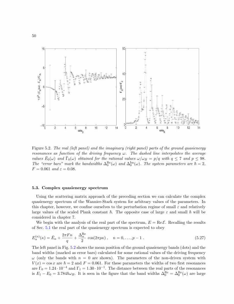
50

Figure 5.2. The real (left panel) and the imaginary (right panel) parts of the ground quasienergyresonances as function of the driving frequency ω. The dashed line interpolates the averagevalues E0(ω) and Γ0(ω) obtained for the rational values ω/ωB = p/q with q ≤ 7 and p ≤ 98.The “error bars” mark the bandwidths ∆Re

0 (ω) and ∆Im0 (ω). The system parameters are ~ = 2,

F = 0.061 and ε = 0.08.

5.3. Complex quasienergy spectrum

Using the scattering matrix approach of the preceding section we can calculate the complexquasienergy spectrum of the Wannier-Stark system for arbitrary values of the parameters. Inthis chapter, however, we confine ourselves to the perturbation regime of small ε and relativelylarge values of the scaled Plank constant ~. The opposite case of large ε and small ~ will beconsidered in chapter 7.

We begin with the analysis of the real part of the spectrum, E = Re E . Recalling the resultsof Sec. 5.1 the real part of the quasienergy spectrum is expected to obey

E(n)α (κ) = Eα +

2πFnq

+∆Reα

2cos(2πpκ) , n = 0, . . . , p− 1 . (5.27)

The left panel in Fig. 5.2 shows the mean position of the ground quasienergy bands (dots) and theband widths (marked as error bars) calculated for some rational values of the driving frequencyω (only the bands with n = 0 are shown). The parameters of the non-driven system withV (x) = cosx are ~ = 2 and F = 0.061. For these parameters the widths of two first resonancesare Γ0 = 1.24 · 10−4 and Γ1 = 1.30 · 10−1. The distance between the real parts of the resonancesis E1 − E0 = 3.784~ωB. It is seen in the figure that the band widths ∆Re

0 = ∆Re0 (ω) are large

51

only for ω = pωB, in qualitative agreement with the estimate (5.11). We would like to stress,however, that estimate (5.11) is obtained within the single-band approximation and, becauseof this, the actual bandwidths deviate from this dependence. (We shall discuss the conditionsof validity of Eq. (5.11) later on in Sec. 5.4.) The second deviation from the predictions ofsingle-band model is the dependence of the mean quasienergy band position E0 on ω. As shownbelow, this dependence reflects the presence of the other quasienergy states, originating fromthe higher (α > 0) Bloch bands. Let us also note that the mean position Eα = Eα(ω) is, unlikethe band width ∆Re

α = ∆Reα (ω), a continuous function of the frequency.

The right panel in Fig. 5.2 shows the imaginary part Γ = −2Im E of the quasienergy spectrum.In the perturbation regime ε→ 0 a behavior similar to (5.27),

Γα(κ) ≈ Γα +∆Imα

2cos(2πκ) , (5.28)

is observed. It should be noted that the smooth function Γ0 = Γ0(ω) approximating the meanvalues of the bands is nothing else as the induced decay rate discussed in Sec. 4.1. In fact, anarbitrary initial state of the system (which was assumed to be the ground Wannier-Stark stateΨ0,l(x) in Sec. 4.1) can be expanded in the basis of the quasienergy states Ψ(n)

α (x) as

Ψ(t = 0) =∑α,n

cα,nΨ(n)α , cα(n) = 〈Ψ(n)

α |Ψ(t = 0)〉 . (5.29)

(Here we assume that ω/ωB is an irrational number and, therefore, the quasienergy functionsare localized function with discrete spectrum.) During the time evolution the coefficients cα,n(t)decay as exp(−Γαt/2~). Since Γα > Γ0 (α > 0), the projection of the wave function back to theinitial state decays (after a short transient) exponentially with an increment given by Γ0(ω)/2.This is the underlying argument of our numerical method of calculating the decay spectrum ofthe system. Namely, to obtain the decay spectrum discussed in chapter 4 we calculated the meanimaginary values of the quasienergy bands for a number of rational ω/ωB and then interpolatethem for an arbitrary ω.

Let us now discuss the ω-dependence of the smooth functions E0(ω), Γ0(ω). Because we ana-lyze the case of weak driving, these functions can be obtained by using perturbation theory. Infact, assuming again an irrational value of ω/ωB, the zero order approximation of the most sta-ble quasienergy function is the ground Wannier-Stark state Ψ0,n(x). According to the commonperturbation theory, the first order correction is

Ψ(n)0 = Ψ0,n + Fω

∑α,l

∑±

〈Ψ0,n|x|Ψα,l〉Eα,l − E0,n ± ~ω

Ψα,l . (5.30)

Correspondingly, the second oder correction to the energy is

E(n)0 = E0,n +

F 2ω

2

∑α,l

∑±

V 20,α(l − n)

Eα − E0 + (l − n)~ωB ± ~ω. (5.31)

In Eq. (5.31) we used the notation (4.3) for the squared dipole matrix elements and took intoaccount that the energies of the Wannier-Stark states form the ladder Eα,l = Eα+l~ωB. Equation(5.31) is illustrated in Fig. 5.3, where the real (left panel) and imaginary (right panel) parts of the

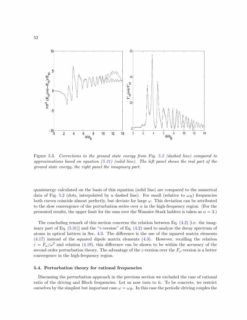
52

Figure 5.3. Corrections to the ground state energy from Fig. 5.2 (dashed line) compared toapproximations based on equation (5.31) (solid line). The left panel shows the real part of theground state energy, the right panel the imaginary part.

quasienergy calculated on the basis of this equation (solid line) are compared to the numericaldata of Fig. 5.2 (dots, interpolated by a dashed line). For small (relative to ωB) frequenciesboth curves coincide almost perfectly, but deviate for large ω. This deviation can be attributedto the slow convergence of the perturbation series over α in the high-frequency region. (For thepresented results, the upper limit for the sum over the Wannier-Stark ladders is taken as α = 3.)

The concluding remark of this section concerns the relation between Eq. (4.2) [i.e. the imag-inary part of Eq. (5.31)] and the “ε-version” of Eq. (4.2) used to analyze the decay spectrum ofatoms in optical lattices in Sec. 4.3. The difference is the use of the squared matrix elements(4.17) instead of the squared dipole matrix elements (4.3). However, recalling the relationε = Fω/ω

2 and relation (4.19), this difference can be shown to be within the accuracy of thesecond order perturbation theory. The advantage of the ε-version over the Fω-version is a betterconvergence in the high-frequency region.

5.4. Perturbation theory for rational frequencies

Discussing the perturbation approach in the previous section we excluded the case of rationalratio of the driving and Bloch frequencies. Let us now turn to it. To be concrete, we restrictourselves by the simplest but important case ω = ωB. In this case the periodic driving couples the

53

Wannier-Stark states belonging to the same Wannier-Stark ladder and, therefore, the extendedWannier-Bloch function Φα,κ is an appropriate zero order approximation to the quasienergyfunction.

As described in the beginning of this chapter, the complex quasienergies of the system arefound by solving the eigenvalue equation

U(Tω)Φα,κ = exp[−iEα(κ)Tω/~] Φα,κ . (5.32)

Let us approximate the Hamiltonian (5.2) by the first order of the Taylor expansion in ε, H ≈HW − ε sin(x) cos(ωt) (here HW is the Wannier-Stark Hamiltonian (2.2) and V (x) = cosx isassumed for simplicity). Then we can calculate the effect of the periodic driving in the interactionrepresentation of the Schrodinger equation. Explicitly, we get

U(Tω) ≈ Uε(Tω)UW (Tω) (5.33)

where the operator Uε(Tω) reads

Uε(Tω) = exp(

iε~

∫ Tω

0dt cos(ωt)U †W (t) sin(x)UW (t)

), (5.34)

and the operator UW (t) is the evolution operator for the unperturbed system. According tocommon perturbation theory, the first order correction is given by the diagonal elements of theoperator Uε(Tω),

exp[−i∆Eα(κ)Tω/~] = 〈Φα,κ|Uε(Tω) |Φα,κ〉 . (5.35)

Let us approximate this formula further. Expanding the operator exponent in a series in ε andkeeping only the first term, the correction to the quasienergy reads

∆Eα(κ) = − ε

Tω

∫ Tω

0dt cos(ωt) 〈Φα,κ|U †W (t) sin(x)UW (t) |Φα,κ〉 . (5.36)

Using the solution UW (t)Φα,κ = exp(−iEαt/~) Φα,κ−Ft/~ and substituting dt/Tω = −dκ,Eq. (5.36) takes the form

∆Eα(κ) = −ε∫ 1

0dκ′ cos(2πκ′) 〈Φα,κ+κ′ | sin(x)|Φα,κ+κ′〉 . (5.37)

Finally, using the symmetry property of the Wannier-Bloch function, the integral (5.37) can bepresented in the form

∆Eα(κ) =(

∆Reα + i∆Im

α

2

)cos(2πκ) , (5.38)

where

∆Reα + i∆Im

α = −2ε∫ 1

0dκ cos(2πκ) 〈Φα,κ| sin(x)|Φα,κ〉 . (5.39)

(The special notation for the band width stresses that the integral on the right hand side ofEq. (5.39) is a complex number.) Thus, a weak periodic driving removes the degeneracy of the

54

Wannier-Bloch bands which then gain a finite width. Moreover, there are corrections both tothe real and imaginary part of the quasienergy.

In conclusion, let us briefly discuss the relation between the formulas (5.38), (5.39) and thetight-binding result (5.12). As was stated many times, the single-band model neglects theinterband tunneling, which is justified in the limit F → 0. In this limit the quasienergy bandwidth can be estimated as

∆Reα = ε

4π2F∆α

~2

= ∆αFωF

, (5.40)

where ∆α is the width of the Bloch band. Indeed, using Eq. (4.18), the band width in Eq. (5.39)can be expressed in terms of the dipole matrix elements as

∆Reα + i∆Im

α = ε(2πF )2

~2

(〈Ψα,1|x|Ψα,0〉+ 〈Ψα,0|x|Ψα,1〉

). (5.41)

Then, using the tight-binding approximation (1.11) for the resonance Wannier-Stark statesΨα,1(x), we obtain the estimate (5.40). (Alternatively, we can approximate χα,κ(x) in Eq. (4.14)by the periodic part of the Bloch function.) It is seen, that the estimate (5.40) coincides withEq. (5.12) in the limit Fω/F → 0. We would like to stress, however, that the actual perturbationparameter of the problem is ε ∼ Fω/F

2 and not Fω/F , as it could be naively expected on thebasis of the tight-binding model.

5.5. Selective decay

This section serves as an illustration to the perturbation theory of Sec. 5.4 and discusses someimportant limitations of the perturbation approach. In order to reduce the number of relevantresonance states, we choose the parameters of the unperturbed system as ~ = 2, F = 0.08. In thiscase we have to take into account mainly two resonances with energies E0 = 9.42·10−2−i5.60·10−4

and E1 = 4.18 · 10−2 − i8.81 · 10−2. All other resonances are very unstable and approximatelydo not influence the results. The frequency of the time-periodic perturbation is given by ω =2πF/~ ≈ 0.251.

Figure 5.4 shows the real parts of the quasienergies of the two most stable Wannier-Blochresonances for different amplitudes ε. In panel (a) we have the unperturbed case with flat bands.When the ac driving is added, the dispersion relation of the ground band is well described by thetheoretical cosine dependence. The first excited band follows this relation only up to ε = 0.2.If the amplitude is increased further, deviations from the cosine appear, and for ε = 1 othereffects strongly influence the band (note that in this case Fω/F ≈ 0.79, thus we are still far awayfrom the parameter range where the tight-binding model predicts dynamical band suppression).Furthermore, for ε > 0.2 the bands cross, and then we cannot neglect their interaction.

Next we investigate the bandwidth, i.e. the difference between the extrema of the real partsof the quasienergies, ∆E = E(κ = 1/2) − E(κ = 0). Figure 5.5 shows the width of the twomost stable bands as a function of the amplitude ε for three different field strengths F = 0.02,F = 0.04 and F = 0.08. It is seen that in all cases the bandwidth grows approximately linearly.Again, the agreement is much better for the ground band; for the first excited band one observesan oscillation around the linear growth. Note that the slope is proportional to F as expectedon the basis of the perturbation theory [see Eq. (5.40)].

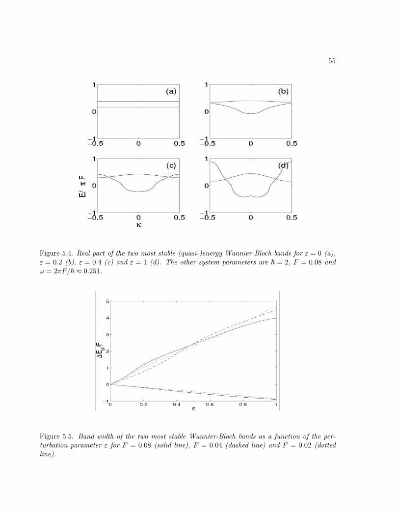
55

Figure 5.4. Real part of the two most stable (quasi-)energy Wannier-Bloch bands for ε = 0 (a),ε = 0.2 (b), ε = 0.4 (c) and ε = 1 (d). The other system parameters are ~ = 2, F = 0.08 andω = 2πF/~ ≈ 0.251.

Figure 5.5. Band width of the two most stable Wannier-Bloch bands as a function of the per-turbation parameter ε for F = 0.08 (solid line), F = 0.04 (dashed line) and F = 0.02 (dottedline).

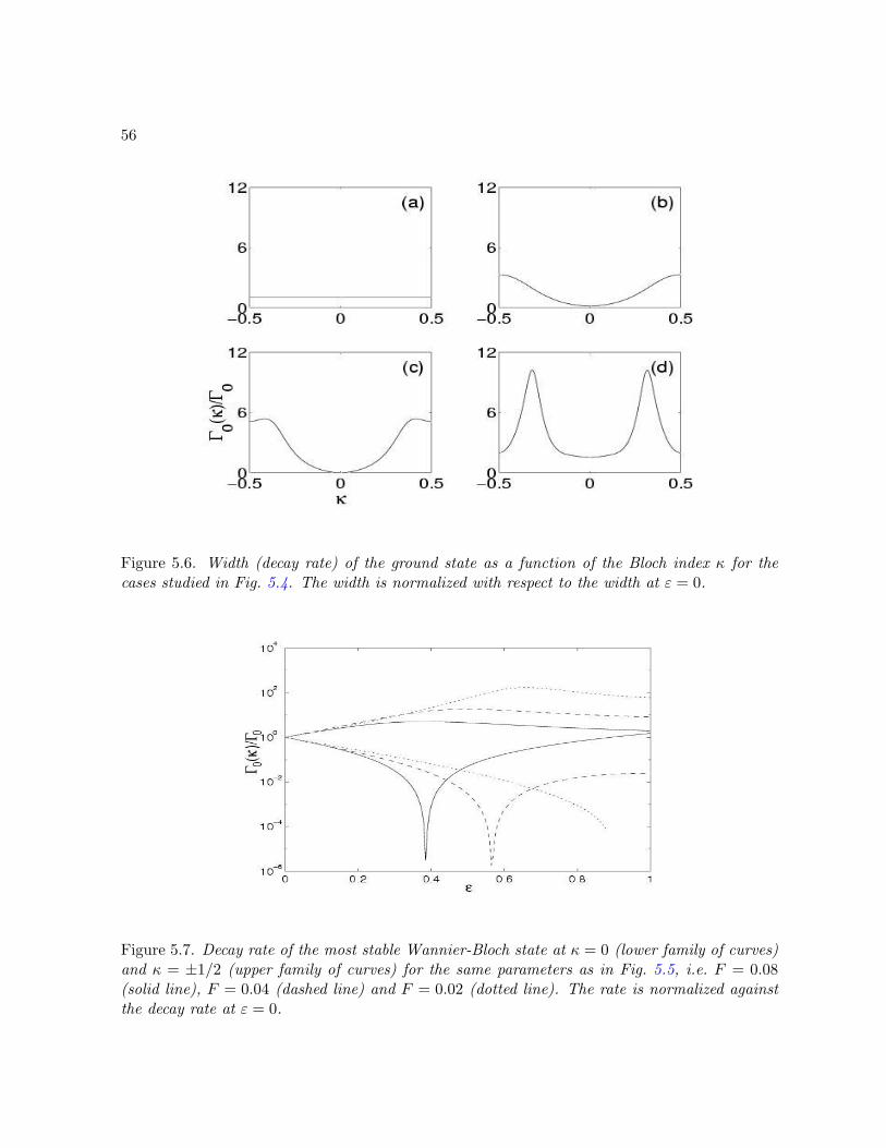
56

Figure 5.6. Width (decay rate) of the ground state as a function of the Bloch index κ for thecases studied in Fig. 5.4. The width is normalized with respect to the width at ε = 0.

Figure 5.7. Decay rate of the most stable Wannier-Bloch state at κ = 0 (lower family of curves)and κ = ±1/2 (upper family of curves) for the same parameters as in Fig. 5.5, i.e. F = 0.08(solid line), F = 0.04 (dashed line) and F = 0.02 (dotted line). The rate is normalized againstthe decay rate at ε = 0.

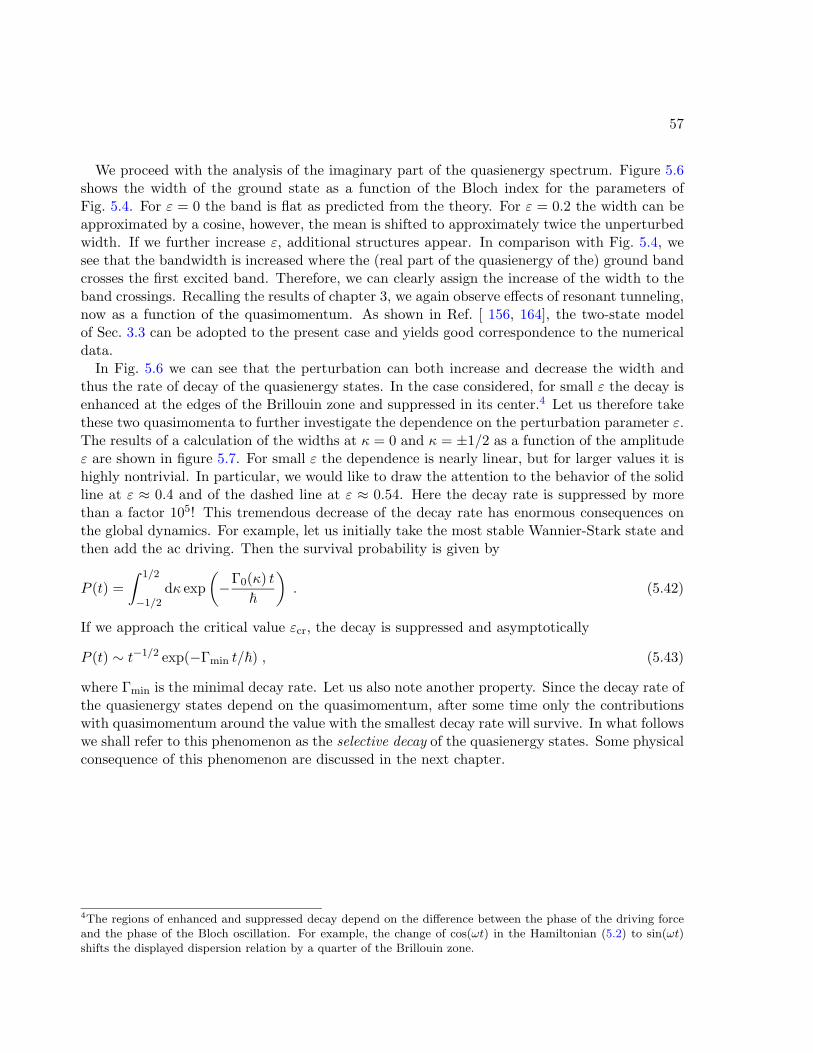
57

We proceed with the analysis of the imaginary part of the quasienergy spectrum. Figure 5.6shows the width of the ground state as a function of the Bloch index for the parameters ofFig. 5.4. For ε = 0 the band is flat as predicted from the theory. For ε = 0.2 the width can beapproximated by a cosine, however, the mean is shifted to approximately twice the unperturbedwidth. If we further increase ε, additional structures appear. In comparison with Fig. 5.4, wesee that the bandwidth is increased where the (real part of the quasienergy of the) ground bandcrosses the first excited band. Therefore, we can clearly assign the increase of the width to theband crossings. Recalling the results of chapter 3, we again observe effects of resonant tunneling,now as a function of the quasimomentum. As shown in Ref. [ 156, 164], the two-state modelof Sec. 3.3 can be adopted to the present case and yields good correspondence to the numericaldata.

In Fig. 5.6 we can see that the perturbation can both increase and decrease the width andthus the rate of decay of the quasienergy states. In the case considered, for small ε the decay isenhanced at the edges of the Brillouin zone and suppressed in its center.4 Let us therefore takethese two quasimomenta to further investigate the dependence on the perturbation parameter ε.The results of a calculation of the widths at κ = 0 and κ = ±1/2 as a function of the amplitudeε are shown in figure 5.7. For small ε the dependence is nearly linear, but for larger values it ishighly nontrivial. In particular, we would like to draw the attention to the behavior of the solidline at ε ≈ 0.4 and of the dashed line at ε ≈ 0.54. Here the decay rate is suppressed by morethan a factor 105! This tremendous decrease of the decay rate has enormous consequences onthe global dynamics. For example, let us initially take the most stable Wannier-Stark state andthen add the ac driving. Then the survival probability is given by

P (t) =∫ 1/2

−1/2dκ exp

(−Γ0(κ) t

~

). (5.42)

If we approach the critical value εcr, the decay is suppressed and asymptotically

P (t) ∼ t−1/2 exp(−Γmin t/~) , (5.43)

where Γmin is the minimal decay rate. Let us also note another property. Since the decay rate ofthe quasienergy states depend on the quasimomentum, after some time only the contributionswith quasimomentum around the value with the smallest decay rate will survive. In what followswe shall refer to this phenomenon as the selective decay of the quasienergy states. Some physicalconsequence of this phenomenon are discussed in the next chapter.

4The regions of enhanced and suppressed decay depend on the difference between the phase of the driving forceand the phase of the Bloch oscillation. For example, the change of cos(ωt) in the Hamiltonian (5.2) to sin(ωt)shifts the displayed dispersion relation by a quarter of the Brillouin zone.

Chapter 6

Wave packet dynamics

In this section we address the question of the time evolution of an initially localized wave packet.Usually this problem is analyzed by simulating the wave packet dynamics on the basis of thetime-dependent Schrodinger equation. However, this numerical approach is very time consumingand has an upper limit for the times considered. In what follows we describe the evolution of thewave packet in terms of the resonance states. Besides tremendous decrease of the computationalefforts, the latter approach also gives additional insight into the decay process of the Wannier-Stark states.

6.1. Expansion over resonance states

A direct expansion of a localized state in terms of resonances yields inappropriate resultsbecause in the negative x-direction the resonance states extend to infinity. Therefore the de-scription needs to be modified to take into account the finite extension of the initial state.Recently this problem was analyzed for decaying quantum systems with a finite range potential[ 183, 184].1

Let us adopt the approach of [ 184] to describe the evolution of the wave packet in momen-tum space. In this approach, the wave function ψ(k, t) is expressed in terms of the stationaryscattering states ΨS(k;E):

ψ(k, t) =∫ ∞−∞

dE f(E) ΨS(k;E) exp(−i

Et

~

), (6.1)

where f(E) = 〈ΨS(k;E)|ψ(k, 0)〉. [We recall that the states ΨS(k;E) are normalized to δ-function: 〈ΨS(k;E′)|ΨS(k;E)〉 = δ(E − E′).] We are mainly interested in the properties ofthe decay tail at k → −∞. In this region the scattering states can be approximated by theirasymptotic form [see Eq. (2.7)]

limk→±∞

Ψ±(k;E) = g±(E) exp(

i~

2k3

6F− i

Ek

F

), g±(E) = e±iϕ(E) . (6.2)

1However, this problem was already addressed in textbooks as, e.g., [ 185].

58

59

Substituting this asymptotic form into Eq. (6.1) we have

ψ(k, t) = exp(

i~

2k3

6F

)G−

(k +

Ft

~

), k 0 , (6.3)

where

G−(k) =∫ ∞−∞

dEf(E)g+(E)

exp(−i

Ek

F

). (6.4)

If the initial wave function ψ(k, 0) has a finite support, f(E) is an entire function in the complexplane. Then the function f(E)/g+(E) has simple poles at zeros of g+(E), i.e at the poles ofthe scattering matrix S(E) = g−(E)/g+(E). This property suggests to evaluate the integral(6.4) with the help of the residuum theorem. Without knowing the explicit form of the functionf(E)/g+(E) we have to make some assumptions on its asymptotic behavior in order to proceedfurther. In particular, if we assume that the function f(E)/g+(E) does not influence the be-havior of the integrand at infinity, the integral yields a sum over the residua located within theappropriate contour. Explicitly, for k > 0 the contour should be closed in the lower half of thecomplex plane, for k < 0 it contains the upper half. Since all poles of the scattering matrix arelocated in the lower half of the complex plane, we get

G−(k) = 2πi Θ (k)∑ν

bν exp(−iEνkF

), (6.5)

where Θ(k) is the Heaviside function, the bν are the residua of f(E)/g+(E) at the poles, andν = α, l. Inserting this result in (6.3) yields

ψ(k, t) = Θ (~k + Ft)∑ν

cν exp[i(~

2k3

6F− Eνk

F− Eνt~

)], (6.6)

with cν = 2πibν . The terms of the sum are actually proportional to the asymptotic form of theresonance wave functions Ψν(k, t). Thus, we can equivalently present the wave function as

ψ(k, t) = Θ (~k + Ft)∑ν

cν exp(−iEνt~

)Ψν(k) . (6.7)

Therefore, in the Stark case we can describe the evolution of an initial state by a superposi-tion of resonances, where we take into account the space-time decay process in the prefactorΘ (~k + Ft). This factor truncates the wave function at the momentum ~k = −Ft, i.e. onlymomenta with ~k > −Ft contribute. With increasing time, the wave function extends to smallermomenta, where the edge moves according to the classical equation of motion.

It should be noted that the location of the edge reflects the assumption on the behaviorat infinity we made in order to explicitly evaluate the integral. For example, the functionf(E)/g+(E) may contain an additional exponential factor exp(iαE) (see the example in [ 184]).Though this factor does not influence the poles, it nevertheless influences the argument of theHeaviside function. In fact, in a realistic situation the edge will be shifted, because the truncationedge at t = 0 has to reflect the extension of the initial state in momentum space. We take thisinto account by replacing ~k in the argument of the Heaviside function by ~(k + k0), where

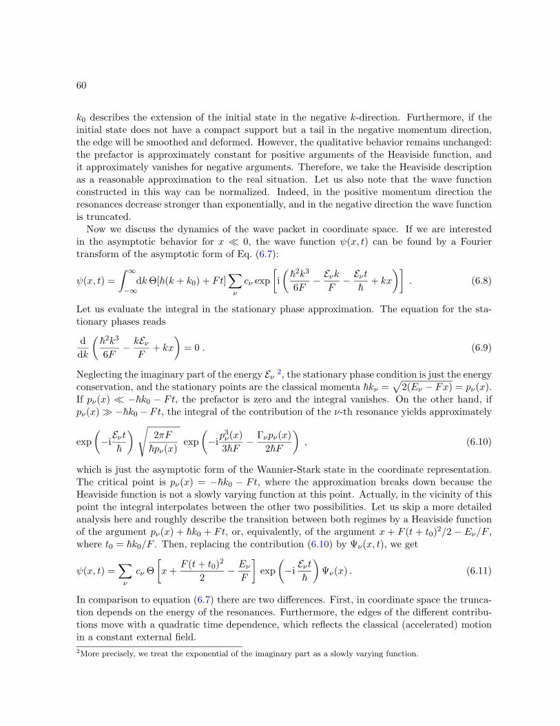
60

k0 describes the extension of the initial state in the negative k-direction. Furthermore, if theinitial state does not have a compact support but a tail in the negative momentum direction,the edge will be smoothed and deformed. However, the qualitative behavior remains unchanged:the prefactor is approximately constant for positive arguments of the Heaviside function, andit approximately vanishes for negative arguments. Therefore, we take the Heaviside descriptionas a reasonable approximation to the real situation. Let us also note that the wave functionconstructed in this way can be normalized. Indeed, in the positive momentum direction theresonances decrease stronger than exponentially, and in the negative direction the wave functionis truncated.

Now we discuss the dynamics of the wave packet in coordinate space. If we are interestedin the asymptotic behavior for x 0, the wave function ψ(x, t) can be found by a Fouriertransform of the asymptotic form of Eq. (6.7):

ψ(x, t) =∫ ∞−∞

dkΘ[~(k + k0) + Ft]∑ν

cν exp[i(~

2k3

6F− Eνk

F− Eνt~

+ kx

)]. (6.8)

Let us evaluate the integral in the stationary phase approximation. The equation for the sta-tionary phases reads

ddk

(~

2k3

6F− kEν

F+ kx

)= 0 . (6.9)

Neglecting the imaginary part of the energy Eν 2, the stationary phase condition is just the energyconservation, and the stationary points are the classical momenta ~kν =

√2(Eν − Fx) = pν(x).

If pν(x) −~k0 − Ft, the prefactor is zero and the integral vanishes. On the other hand, ifpν(x) −~k0 − Ft, the integral of the contribution of the ν-th resonance yields approximately

exp(−iEνt~

) √2πF~pν(x)

exp(−ip3ν(x)3~F

− Γνpν(x)2~F

), (6.10)

which is just the asymptotic form of the Wannier-Stark state in the coordinate representation.The critical point is pν(x) = −~k0 − Ft, where the approximation breaks down because theHeaviside function is not a slowly varying function at this point. Actually, in the vicinity of thispoint the integral interpolates between the other two possibilities. Let us skip a more detailedanalysis here and roughly describe the transition between both regimes by a Heaviside functionof the argument pν(x) + ~k0 + Ft, or, equivalently, of the argument x + F (t + t0)2/2 − Eν/F ,where t0 = ~k0/F . Then, replacing the contribution (6.10) by Ψν(x, t), we get

ψ(x, t) =∑ν

cν Θ[x+

F (t+ t0)2

2− Eν

F

]exp

(−iEνt~

)Ψν(x) . (6.11)

In comparison to equation (6.7) there are two differences. First, in coordinate space the trunca-tion depends on the energy of the resonances. Furthermore, the edges of the different contribu-tions move with a quadratic time dependence, which reflects the classical (accelerated) motionin a constant external field.2More precisely, we treat the exponential of the imaginary part as a slowly varying function.

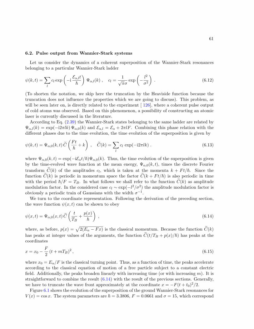
61

6.2. Pulse output from Wannier-Stark systems

Let us consider the dynamics of a coherent superposition of the Wannier-Stark resonancesbelonging to a particular Wannier-Stark ladder

ψ(k, t) =∑l

cl exp(−iEα,lt~

)Ψα,l(k) , cl =

1√πσ

exp(− l

2

σ2

). (6.12)

(To shorten the notation, we skip here the truncation by the Heaviside function because thetruncation does not influence the properties which we are going to discuss). This problem, aswill be seen later on, is directly related to the experiment [ 126], where a coherent pulse outputof cold atoms was observed. Based on this phenomenon, a possibility of constructing an atomiclaser is currently discussed in the literature.

According to Eq. (2.39) the Wannier-Stark states belonging to the same ladder are related byΨα,l(k) = exp(−i2πlk) Ψα,0(k) and Eα,l = Eα + 2πlF . Combining this phase relation with thedifferent phases due to the time evolution, the time evolution of the superposition is given by

ψ(k, t) = Ψα,0(k, t) C(Ft

~

+ k

), C(k) =

∑l

cl exp(−i2πlk) . (6.13)

where Ψα,0(k, t) = exp(−iEαt/~)Ψα,0(k). Thus, the time evolution of the superposition is givenby the time-evolved wave function at the mean energy, Ψα,0(k, t), times the discrete Fouriertransform C(k) of the amplitudes cl, which is taken at the momenta k + Ft/~. Since thefunction C(k) is periodic in momentum space the factor C(k + Ft/~) is also periodic in timewith the period ~/F = TB. In what follows we shall refer to the function C(k) as amplitudemodulation factor. In the considered case cl ∼ exp(−l2/σ2) the amplitude modulation factor isobviously a periodic train of Gaussians with the width σ−1.

We turn to the coordinate representation. Following the derivation of the preceding section,the wave function ψ(x, t) can be shown to obey

ψ(x, t) = Ψα,0(x, t) C(t

TB+p(x)~

), (6.14)

where, as before, p(x) =√

2(Eα − Fx) is the classical momentum. Because the function C(k)has peaks at integer values of the arguments, the function C(t/TB + p(x)/~) has peaks at thecoordinates

x = x0 −F

2(t+mTB)2 , (6.15)

where x0 = Eα/F is the classical turning point. Thus, as a function of time, the peaks accelerateaccording to the classical equation of motion of a free particle subject to a constant electricfield. Additionally, the peaks broaden linearly with increasing time (or with increasing m). It isstraightforward to combine the result (6.14) with the result of the previous sections. Generally,we have to truncate the wave front approximately at the coordinate x = −F (t+ t0)2/2.

Figure 6.1 shows the evolution of the superposition of the ground Wannier-Stark resonances forV (x) = cosx. The system parameters are ~ = 3.3806, F = 0.0661 and σ = 15, which correspond

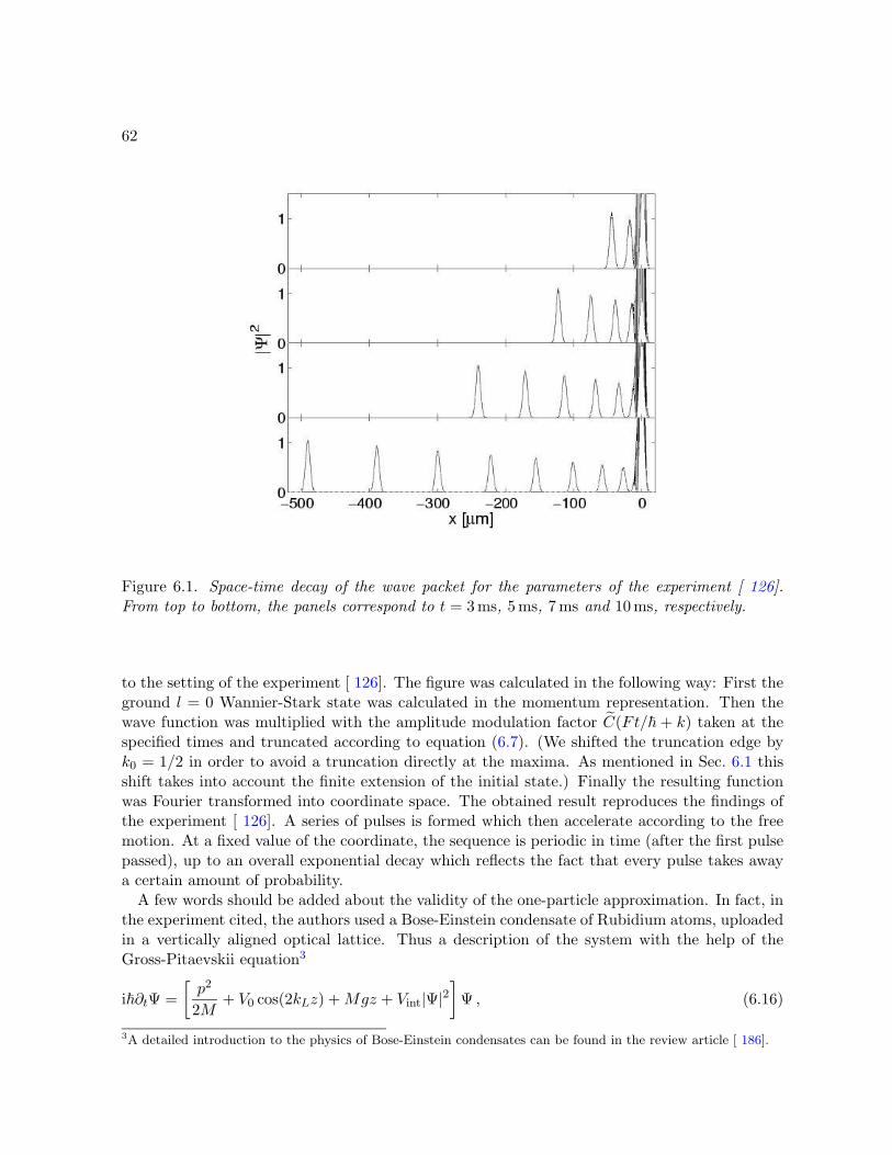
62

Figure 6.1. Space-time decay of the wave packet for the parameters of the experiment [ 126].From top to bottom, the panels correspond to t = 3 ms, 5 ms, 7 ms and 10 ms, respectively.

to the setting of the experiment [ 126]. The figure was calculated in the following way: First theground l = 0 Wannier-Stark state was calculated in the momentum representation. Then thewave function was multiplied with the amplitude modulation factor C(Ft/~ + k) taken at thespecified times and truncated according to equation (6.7). (We shifted the truncation edge byk0 = 1/2 in order to avoid a truncation directly at the maxima. As mentioned in Sec. 6.1 thisshift takes into account the finite extension of the initial state.) Finally the resulting functionwas Fourier transformed into coordinate space. The obtained result reproduces the findings ofthe experiment [ 126]. A series of pulses is formed which then accelerate according to the freemotion. At a fixed value of the coordinate, the sequence is periodic in time (after the first pulsepassed), up to an overall exponential decay which reflects the fact that every pulse takes awaya certain amount of probability.

A few words should be added about the validity of the one-particle approximation. In fact, inthe experiment cited, the authors used a Bose-Einstein condensate of Rubidium atoms, uploadedin a vertically aligned optical lattice. Thus a description of the system with the help of theGross-Pitaevskii equation3

i~∂tΨ =[p2

2M+ V0 cos(2kLz) +Mgz + Vint|Ψ|2

]Ψ , (6.16)

3A detailed introduction to the physics of Bose-Einstein condensates can be found in the review article [ 186].

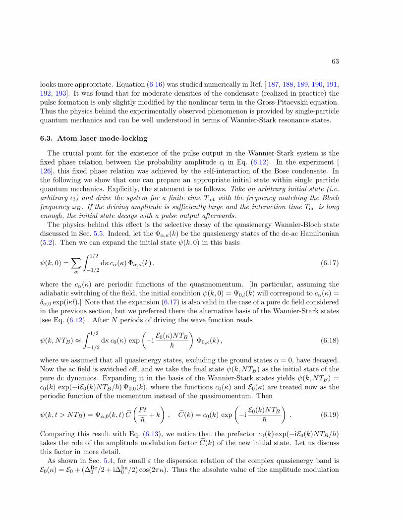
63

looks more appropriate. Equation (6.16) was studied numerically in Ref. [ 187, 188, 189, 190, 191,192, 193]. It was found that for moderate densities of the condensate (realized in practice) thepulse formation is only slightly modified by the nonlinear term in the Gross-Pitaevskii equation.Thus the physics behind the experimentally observed phenomenon is provided by single-particlequantum mechanics and can be well understood in terms of Wannier-Stark resonance states.

6.3. Atom laser mode-locking

The crucial point for the existence of the pulse output in the Wannier-Stark system is thefixed phase relation between the probability amplitude cl in Eq. (6.12). In the experiment [126], this fixed phase relation was achieved by the self-interaction of the Bose condensate. Inthe following we show that one can prepare an appropriate initial state within single particlequantum mechanics. Explicitly, the statement is as follows. Take an arbitrary initial state (i.e.arbitrary cl) and drive the system for a finite time Tint with the frequency matching the Blochfrequency ωB. If the driving amplitude is sufficiently large and the interaction time Tint is longenough, the initial state decays with a pulse output afterwards.

The physics behind this effect is the selective decay of the quasienergy Wannier-Bloch statediscussed in Sec. 5.5. Indeed, let the Φα,κ(k) be the quasienergy states of the dc-ac Hamiltonian(5.2). Then we can expand the initial state ψ(k, 0) in this basis

ψ(k, 0) =∑α

∫ 1/2

−1/2dκ cα(κ) Φα,κ(k) , (6.17)

where the cα(κ) are periodic functions of the quasimomentum. [In particular, assuming theadiabatic switching of the field, the initial condition ψ(k, 0) = Ψ0,l(k) will correspond to cα(κ) =δα,0 exp(iκl).] Note that the expansion (6.17) is also valid in the case of a pure dc field consideredin the previous section, but we preferred there the alternative basis of the Wannier-Stark states[see Eq. (6.12)]. After N periods of driving the wave function reads

ψ(k,NTB) ≈∫ 1/2

−1/2dκ c0(κ) exp

(−iE0(κ)NTB

~

)Φ0,κ(k) , (6.18)

where we assumed that all quasienergy states, excluding the ground states α = 0, have decayed.Now the ac field is switched off, and we take the final state ψ(k,NTB) as the initial state of thepure dc dynamics. Expanding it in the basis of the Wannier-Stark states yields ψ(k,NTB) =c0(k) exp(−iE0(k)NTB/~) Ψ0,0(k), where the functions c0(κ) and E0(κ) are treated now as theperiodic function of the momentum instead of the quasimomentum. Then

ψ(k, t > NTB) = Ψα,0(k, t) C(Ft

~

+ k

), C(k) = c0(k) exp

(−iE0(k)NTB

~

). (6.19)

Comparing this result with Eq. (6.13), we notice that the prefactor c0(k) exp(−iE0(k)NTB/~)takes the role of the amplitude modulation factor C(k) of the new initial state. Let us discussthis factor in more detail.

As shown in Sec. 5.4, for small ε the dispersion relation of the complex quasienergy band isE0(κ) = E0 + (∆Re

0 /2 + i∆Im0 /2) cos(2πκ). Thus the absolute value of the amplitude modulation

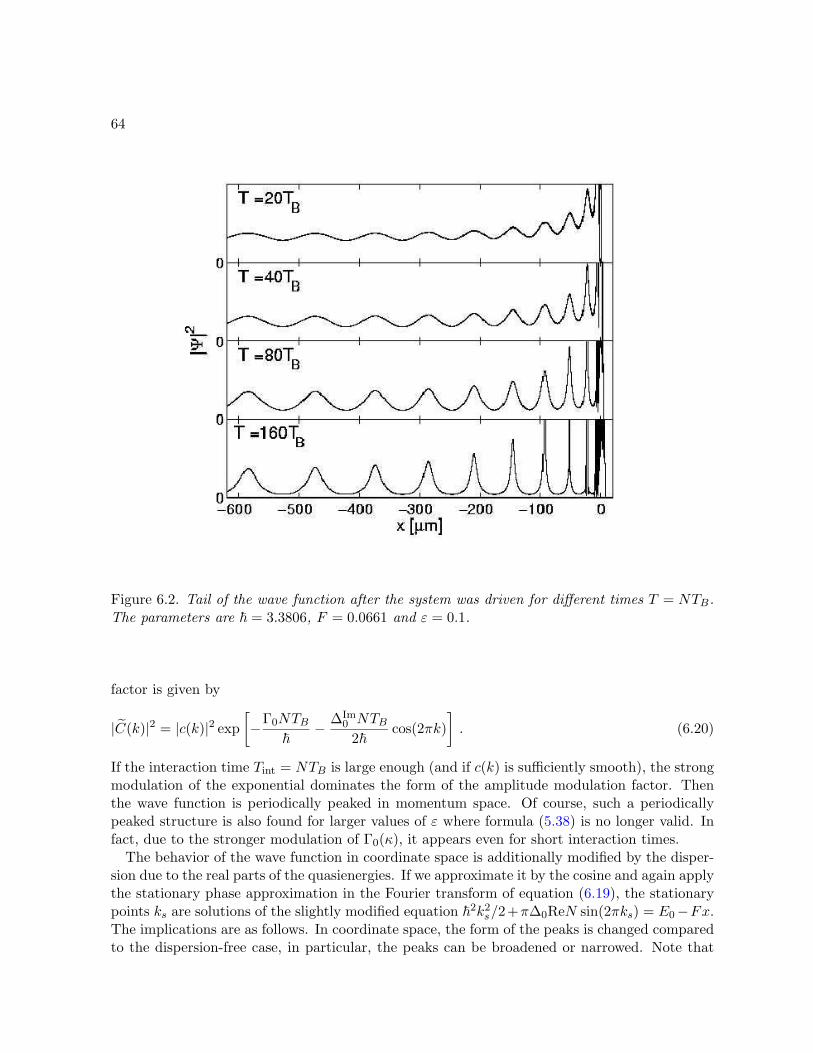
64

Figure 6.2. Tail of the wave function after the system was driven for different times T = NTB.The parameters are ~ = 3.3806, F = 0.0661 and ε = 0.1.

factor is given by

|C(k)|2 = |c(k)|2 exp[−Γ0NTB

~

− ∆Im0 NTB

2~cos(2πk)

]. (6.20)

If the interaction time Tint = NTB is large enough (and if c(k) is sufficiently smooth), the strongmodulation of the exponential dominates the form of the amplitude modulation factor. Thenthe wave function is periodically peaked in momentum space. Of course, such a periodicallypeaked structure is also found for larger values of ε where formula (5.38) is no longer valid. Infact, due to the stronger modulation of Γ0(κ), it appears even for short interaction times.

The behavior of the wave function in coordinate space is additionally modified by the disper-sion due to the real parts of the quasienergies. If we approximate it by the cosine and again applythe stationary phase approximation in the Fourier transform of equation (6.19), the stationarypoints ks are solutions of the slightly modified equation ~2k2

s/2+π∆0ReN sin(2πks) = E0−Fx.The implications are as follows. In coordinate space, the form of the peaks is changed comparedto the dispersion-free case, in particular, the peaks can be broadened or narrowed. Note that

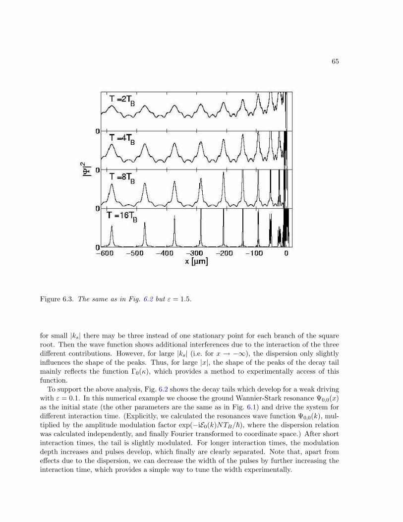
65

Figure 6.3. The same as in Fig. 6.2 but ε = 1.5.

for small |ks| there may be three instead of one stationary point for each branch of the squareroot. Then the wave function shows additional interferences due to the interaction of the threedifferent contributions. However, for large |ks| (i.e. for x → −∞), the dispersion only slightlyinfluences the shape of the peaks. Thus, for large |x|, the shape of the peaks of the decay tailmainly reflects the function Γ0(κ), which provides a method to experimentally access of thisfunction.

To support the above analysis, Fig. 6.2 shows the decay tails which develop for a weak drivingwith ε = 0.1. In this numerical example we choose the ground Wannier-Stark resonance Ψ0,0(x)as the initial state (the other parameters are the same as in Fig. 6.1) and drive the system fordifferent interaction time. (Explicitly, we calculated the resonances wave function Ψ0,0(k), mul-tiplied by the amplitude modulation factor exp(−iE0(k)NTB/~), where the dispersion relationwas calculated independently, and finally Fourier transformed to coordinate space.) After shortinteraction times, the tail is slightly modulated. For longer interaction times, the modulationdepth increases and pulses develop, which finally are clearly separated. Note that, apart fromeffects due to the dispersion, we can decrease the width of the pulses by further increasing theinteraction time, which provides a simple way to tune the width experimentally.

66

A crucial point of the weak driving regime is the long interaction time which is needed togenerate well separated pulses. The relevant timescale is set by the most long-lived state fromthe ground band. For the case ε = 0.1, the minimum width is Γmin = 7.214 · 10−3, whichcorresponds to a lifetime approximately 10TB. Thus, the interaction time is much longer thanthe lifetime of the most stable state. Consequently, a predominant part of the initial wave packethas already decayed before pulses are being formed. One can, however, surmount this problemby increasing the amplitude of the resonant driving. Figure 6.3 shows the decay tail for ε = 1.5.Now the pulses develop after much shorter interaction times. For ε = 1.5, the function Γ0(κ)has four minima, which are due to two crossings with higher excited Wannier-Stark ladders (seeSec. 5.4). Note that one can directly read off this property from the substructure of the pulseson the decay tail. In the lower panels of the figure one can also see the narrowing caused bythe dispersion. In particular, the first peaks (counted from the right) strongly oscillate, whichreflects the existence of three stationary points in this region. However, the last peaks haveapproximately the same shape, i.e. here the narrowing effect can be neglected.

Chapter 7

Chaotic scattering

This chapter continues the analysis of Wannier-Stark system affected by an ac field. In chapters5-6 we have considered the case of a relatively large scaled Planck constant ~ (see Sec. 1.4) andrelatively small values of driving amplitude ε, where the perturbation approach can be applied toanalyze the spectral and dynamical properties of the system. Now we turn to the region of small~ → 0. In this region even a weak driving violates the condition of perturbation theory whichroughly reads ε/~ < 1. On the other hand, a small ~ corresponds to the semiclassical region,where the classical mechanics can guide the quantum-mechanical analysis. It turns out (see nextsection) that the classical dynamics of the system (5.2) is typically chaotic. Then the questionwe address sounds as “What are the quantum manifestations of this chaotic dynamics?”. Thisquestion belongs to the list of problems considered by the modern branch of quantum mechanicsknown as Quantum Chaos (and actually can be considered as the definition of the field) [ 194].

A powerful tool of the theory of quantum chaos is the random matrix theory (RMT) [194, 195, 196, 197]. Its application is based on the conjecture that the spectral propertiesof a classically chaotic system are similar to those of a random matrix of the same (as theHamiltonian) symmetry class. Recently a considerable progress has been made in nonhermitianrandom matrix theory, which aims at describing the properties of chaotic scattering systems [198, 199, 200, 201, 202]. In what follows we study the system (5.2) from the point of view ofnonhermitian random matrix theory. In particular, we numerically calculate the distributionof the width of the quasienergy Wannier-Stark resonances and distribution of the Wigner de-lay time and compare them with the prediction of RMT. We would like to note that presentlythere are just a few physical models which allow a detailed comparison with analytical resultsof RMT.1 In this context, the driven Wannier-Stark system (5.2),

H =p2

2+ cos[x+ ε cos(ωt)] + Fx , ε =

Fωω2

, (7.1)

(to be concrete, we choose V (x) = cosx) serves an excellent example for testing an abstractRMT.

1Among the physical models, two-dimensional billiards with attached leads [ 203, 204, 205], simplified models ofatomic and molecular systems [ 206, 207, 208], the kicked rotor with absorbing boundary condition [ 209, 210, 211],and scattering on graphs [ 212, 213] could be mentioned.

67

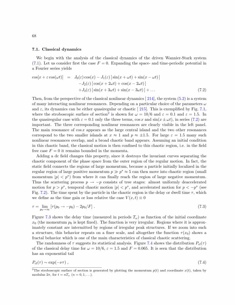
68

7.1. Classical dynamics

We begin with the analysis of the classical dynamics of the driven Wannier-Stark system(7.1). Let us consider first the case F = 0. Expanding the space- and time-periodic potential ina Fourier series yields

cos[x+ ε cos(ωt)] = J0(ε) cos(x)− J1(ε) [ sin(x+ ωt) + sin(x− ωt) ]−J2(ε) [ cos(x+ 2ωt) + cos(x− 2ωt) ]+J3(ε) [ sin(x+ 3ωt) + sin(x− 3ωt) ] + . . . (7.2)

Then, from the perspective of the classical nonlinear dynamics [ 214], the system (5.2) is a systemof many interacting nonlinear resonances. Depending on a particular choice of the parameters ωand ε, its dynamics can be either quasiregular or chaotic [ 215]. This is exemplified by Fig. 7.1,where the stroboscopic surface of section2 is shown for ω = 10/6 and ε = 0.1 and ε = 1.5. Inthe quasiregular case with ε = 0.1 only the three terms, cosx and sin(x±ωt), in series (7.2) areimportant. The three corresponding nonlinear resonances are clearly visible in the left panel.The main resonance of cosx appears as the large central island and the two other resonancescorrespond to the two smaller islands at x ≈ 1 and p ≈ ±1.5. For large ε = 1.5 many suchnonlinear resonances overlap, and a broad chaotic band appears. Assuming an initial conditionin this chaotic band, the classical motion is then confined to this chaotic region, i.e. in the fieldfree case F = 0 it remains bounded in the momenta.

Adding a dc field changes this property, since it destroys the invariant curves separating thechaotic component of the phase space from the outer region of the regular motion. In fact, thestatic field connects the regions of large momentum, because a particle initially localized in theregular region of large positive momentum p p∗ ≈ 5 can then move into chaotic region (smallmomentum |p| < p∗) from where it can finally reach the region of large negative momentum.Thus the scattering process p → −p consists of tree stages: almost uniformly deacceleratedmotion for p > p∗, temporal chaotic motion |p| < p∗, and accelerated motion for p < −p∗ (seeFig. 7.2). The time spent by the particle in the chaotic region is the delay or dwell time τ , whichwe define as the time gain or loss relative the case V (x, t) ≡ 0

τ = limp0→∞

[τ(p0 → −p0)− 2p0/F ] . (7.3)

Figure 7.3 shows the delay time (measured in periods Tω) as function of the initial coordinatex0 (the momentum p0 is kept fixed). The function is very irregular. Regions where it is approx-imately constant are intermitted by regions of irregular peak structures. If we zoom into sucha structure, this behavior repeats on a finer scale, and altogether the function τ(x0) shows afractal behavior which is one of the main characteristics of classical chaotic scattering.

The randomness of τ suggests its statistical analysis. Figure 7.4 shows the distribution Pcl(τ)of the classical delay time for ω = 10/6, ε = 1.5 and F = 0.065. It is seen that the distributionhas an exponential tail

Pcl(τ) ∼ exp(−ντ) , (7.4)

2The stroboscopic surface of section is generated by plotting the momentum p(t) and coordinate x(t), taken bymodulus 2π, for t = nTω (n = 0, 1, . . .).

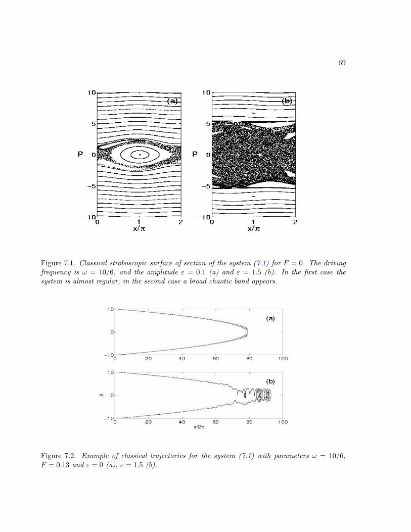
69

Figure 7.1. Classical stroboscopic surface of section of the system (7.1) for F = 0. The drivingfrequency is ω = 10/6, and the amplitude ε = 0.1 (a) and ε = 1.5 (b). In the first case thesystem is almost regular, in the second case a broad chaotic band appears.

Figure 7.2. Example of classical trajectories for the system (7.1) with parameters ω = 10/6,F = 0.13 and ε = 0 (a), ε = 1.5 (b).

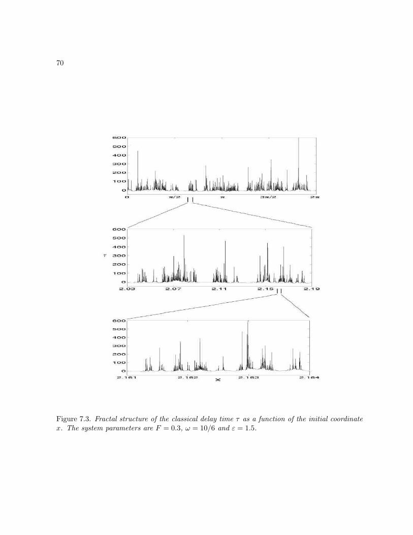
70

Figure 7.3. Fractal structure of the classical delay time τ as a function of the initial coordinatex. The system parameters are F = 0.3, ω = 10/6 and ε = 1.5.

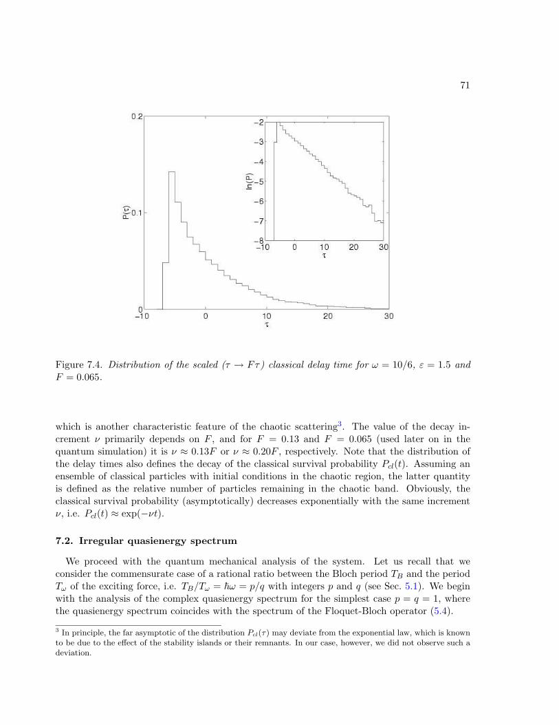
71

Figure 7.4. Distribution of the scaled (τ → Fτ) classical delay time for ω = 10/6, ε = 1.5 andF = 0.065.

which is another characteristic feature of the chaotic scattering3. The value of the decay in-crement ν primarily depends on F , and for F = 0.13 and F = 0.065 (used later on in thequantum simulation) it is ν ≈ 0.13F or ν ≈ 0.20F , respectively. Note that the distribution ofthe delay times also defines the decay of the classical survival probability Pcl(t). Assuming anensemble of classical particles with initial conditions in the chaotic region, the latter quantityis defined as the relative number of particles remaining in the chaotic band. Obviously, theclassical survival probability (asymptotically) decreases exponentially with the same incrementν, i.e. Pcl(t) ≈ exp(−νt).

7.2. Irregular quasienergy spectrum

We proceed with the quantum mechanical analysis of the system. Let us recall that weconsider the commensurate case of a rational ratio between the Bloch period TB and the periodTω of the exciting force, i.e. TB/Tω = ~ω = p/q with integers p and q (see Sec. 5.1). We beginwith the analysis of the complex quasienergy spectrum for the simplest case p = q = 1, wherethe quasienergy spectrum coincides with the spectrum of the Floquet-Bloch operator (5.4).

3 In principle, the far asymptotic of the distribution Pcl(τ) may deviate from the exponential law, which is knownto be due to the effect of the stability islands or their remnants. In our case, however, we did not observe such adeviation.

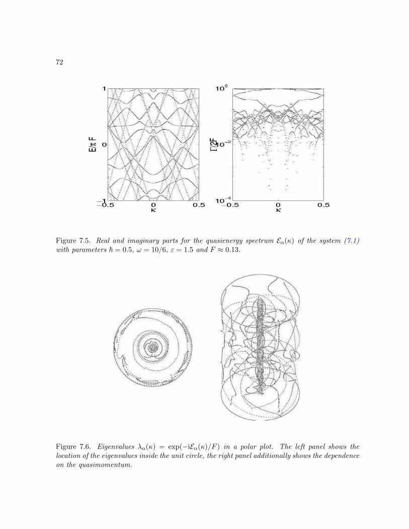
72

Figure 7.5. Real and imaginary parts for the quasienergy spectrum Eα(κ) of the system (7.1)with parameters ~ = 0.5, ω = 10/6, ε = 1.5 and F ≈ 0.13.

Figure 7.6. Eigenvalues λα(κ) = exp(−iEα(κ)/F ) in a polar plot. The left panel shows thelocation of the eigenvalues inside the unit circle, the right panel additionally shows the dependenceon the quasimomentum.

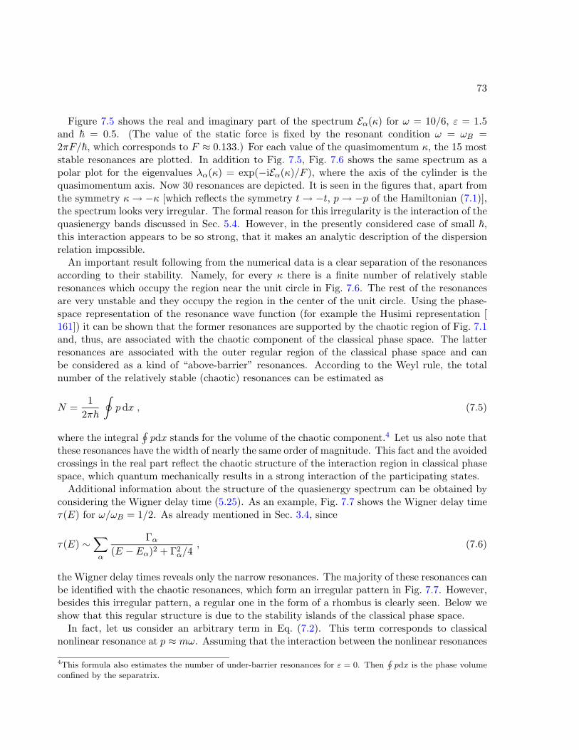
73

Figure 7.5 shows the real and imaginary part of the spectrum Eα(κ) for ω = 10/6, ε = 1.5and ~ = 0.5. (The value of the static force is fixed by the resonant condition ω = ωB =2πF/~, which corresponds to F ≈ 0.133.) For each value of the quasimomentum κ, the 15 moststable resonances are plotted. In addition to Fig. 7.5, Fig. 7.6 shows the same spectrum as apolar plot for the eigenvalues λα(κ) = exp(−iEα(κ)/F ), where the axis of the cylinder is thequasimomentum axis. Now 30 resonances are depicted. It is seen in the figures that, apart fromthe symmetry κ→ −κ [which reflects the symmetry t→ −t, p→ −p of the Hamiltonian (7.1)],the spectrum looks very irregular. The formal reason for this irregularity is the interaction of thequasienergy bands discussed in Sec. 5.4. However, in the presently considered case of small ~,this interaction appears to be so strong, that it makes an analytic description of the dispersionrelation impossible.

An important result following from the numerical data is a clear separation of the resonancesaccording to their stability. Namely, for every κ there is a finite number of relatively stableresonances which occupy the region near the unit circle in Fig. 7.6. The rest of the resonancesare very unstable and they occupy the region in the center of the unit circle. Using the phase-space representation of the resonance wave function (for example the Husimi representation [161]) it can be shown that the former resonances are supported by the chaotic region of Fig. 7.1and, thus, are associated with the chaotic component of the classical phase space. The latterresonances are associated with the outer regular region of the classical phase space and canbe considered as a kind of “above-barrier” resonances. According to the Weyl rule, the totalnumber of the relatively stable (chaotic) resonances can be estimated as

N =1

2π~

∮p dx , (7.5)

where the integral∮pdx stands for the volume of the chaotic component.4 Let us also note that

these resonances have the width of nearly the same order of magnitude. This fact and the avoidedcrossings in the real part reflect the chaotic structure of the interaction region in classical phasespace, which quantum mechanically results in a strong interaction of the participating states.

Additional information about the structure of the quasienergy spectrum can be obtained byconsidering the Wigner delay time (5.25). As an example, Fig. 7.7 shows the Wigner delay timeτ(E) for ω/ωB = 1/2. As already mentioned in Sec. 3.4, since

τ(E) ∼∑α

Γα(E − Eα)2 + Γ2

α/4, (7.6)

the Wigner delay times reveals only the narrow resonances. The majority of these resonances canbe identified with the chaotic resonances, which form an irregular pattern in Fig. 7.7. However,besides this irregular pattern, a regular one in the form of a rhombus is clearly seen. Below weshow that this regular structure is due to the stability islands of the classical phase space.

In fact, let us consider an arbitrary term in Eq. (7.2). This term corresponds to classicalnonlinear resonance at p ≈ mω. Assuming that the interaction between the nonlinear resonances

4This formula also estimates the number of under-barrier resonances for ε = 0. Then∮pdx is the phase volume

confined by the separatrix.

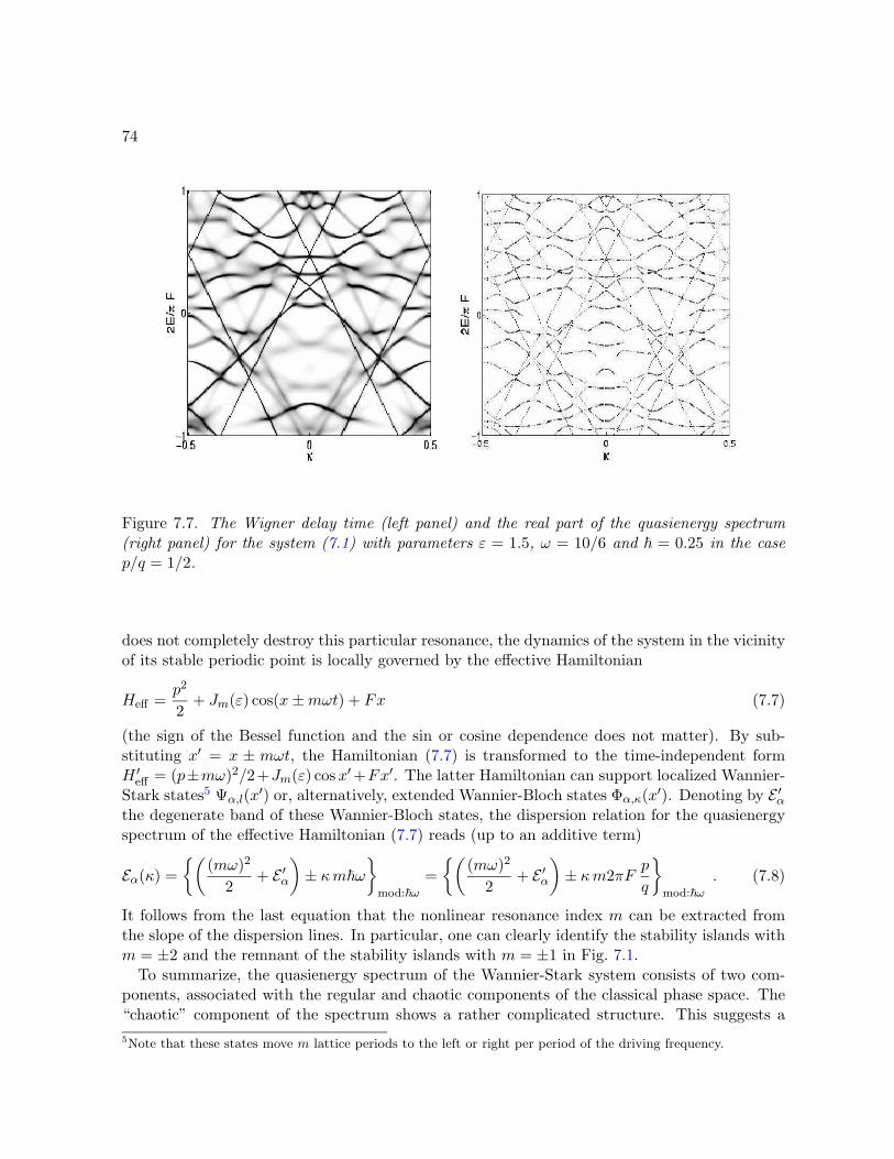
74

Figure 7.7. The Wigner delay time (left panel) and the real part of the quasienergy spectrum(right panel) for the system (7.1) with parameters ε = 1.5, ω = 10/6 and ~ = 0.25 in the casep/q = 1/2.

does not completely destroy this particular resonance, the dynamics of the system in the vicinityof its stable periodic point is locally governed by the effective Hamiltonian

Heff =p2

2+ Jm(ε) cos(x±mωt) + Fx (7.7)

(the sign of the Bessel function and the sin or cosine dependence does not matter). By sub-stituting x′ = x ± mωt, the Hamiltonian (7.7) is transformed to the time-independent formH ′eff = (p±mω)2/2+Jm(ε) cosx′+Fx′. The latter Hamiltonian can support localized Wannier-Stark states5 Ψα,l(x′) or, alternatively, extended Wannier-Bloch states Φα,κ(x′). Denoting by E ′αthe degenerate band of these Wannier-Bloch states, the dispersion relation for the quasienergyspectrum of the effective Hamiltonian (7.7) reads (up to an additive term)

Eα(κ) =(

(mω)2

2+ E ′α

)± κm~ω

mod:~ω

=(

(mω)2

2+ E ′α

)± κm2πF

p

q

mod:~ω

. (7.8)

It follows from the last equation that the nonlinear resonance index m can be extracted fromthe slope of the dispersion lines. In particular, one can clearly identify the stability islands withm = ±2 and the remnant of the stability islands with m = ±1 in Fig. 7.1.

To summarize, the quasienergy spectrum of the Wannier-Stark system consists of two com-ponents, associated with the regular and chaotic components of the classical phase space. The“chaotic” component of the spectrum shows a rather complicated structure. This suggests a5Note that these states move m lattice periods to the left or right per period of the driving frequency.

75

statistical analysis of the spectrum, which will be done in Sec. 7.4. Before doing this, however,we shall briefly discuss some results of random matrix theory.

7.3. Random matrix model

As was mentioned in the introductory part of this chapter, the main conjecture of randommatrix theory of quantum chaos is that the spectral statistics of a classically chaotic systemcoincides with those of an appropriate ensemble of the random matrix. Let us first discusswhich ensemble is “appropriate” to model the spectral statistics of the system of our interest.

According to the results of Sec. 5.2, the quasienergy resonances of the Wannier-Stark systemare given by the eigenvalues of the nonunitary matrix (5.17), which enters in the definition ofthe scattering matrix (5.23). In the random matrix approach it is reasonable to keep the samestructure of the matrix. In other words, we model the case of rational ω/ωB = p/q by therandom scattering matrix

S(E) = eM [B − e−iE11]−1eM , eM =(ON,M 11M,M

), eM =

(11M,M

ON,M

), (7.9)

where nonunitary matrix B is given by

B =

(OM,N OM,M

WN,N ON,M

), (7.10)

and WN,N is a random unitary matrix of size N ×N . In Eq. (7.9) and Eq. (7.10), the parameterM is identical with the denominator q in the condition of comensurability.6 Moreover, we chooseWN,N to be a member of Circular Unitary Ensemble (CUE). The reason for this is that matrixWN,N should model the unitary matrix U (κ),

U (κ) = exp(− i~

∫ T

0dt[

(p+ ~κ− Ft)2

2+ V (x, t)

])(7.11)

which, excluding the cases κ = 0 and κ = ±1/2, has no time-reversal symmetry.Now we discuss the statistics of the resonance widths. The histograms in the left panel of

Fig. 7.8 show the distribution of the scaled resonance widths for the random matrix model (7.9),(7.10) for M = 1, 2, 3. These histograms are obtained in the following way. First, we generatea random 40 × 40 GOE (Gaussian Orthogonal Ensemble) matrix, i.e., a symmetric matrixwith Gaussian-distributed random elements. Then, multiplying the eigenvectors of this matrix(arranged column-wise in a square matrix) by a random-phase factor, we obtain a member ofCUE [ 216]. This CUE matrix is enlarged to a nonunitary matrix B and diagonalized. Afterdiagonalization, we have (N −M) non-zero eigenvalues λ = exp[−i(E − iΓ/2)]. To ensure theconvergence in the limit N → ∞, the resonance widths Γ are scaled based on the mean levelspacing ∆ = 2π/(N −M) as Γs = NΓ/2 ≈ πΓ/∆. Finally, the distribution of the scaled widthsis calculated for an ensemble of 1000 random matrices.6 In this section, we use the standard notation of RMT, i.e. N for the matrix size and M for the number ofscattering channels.

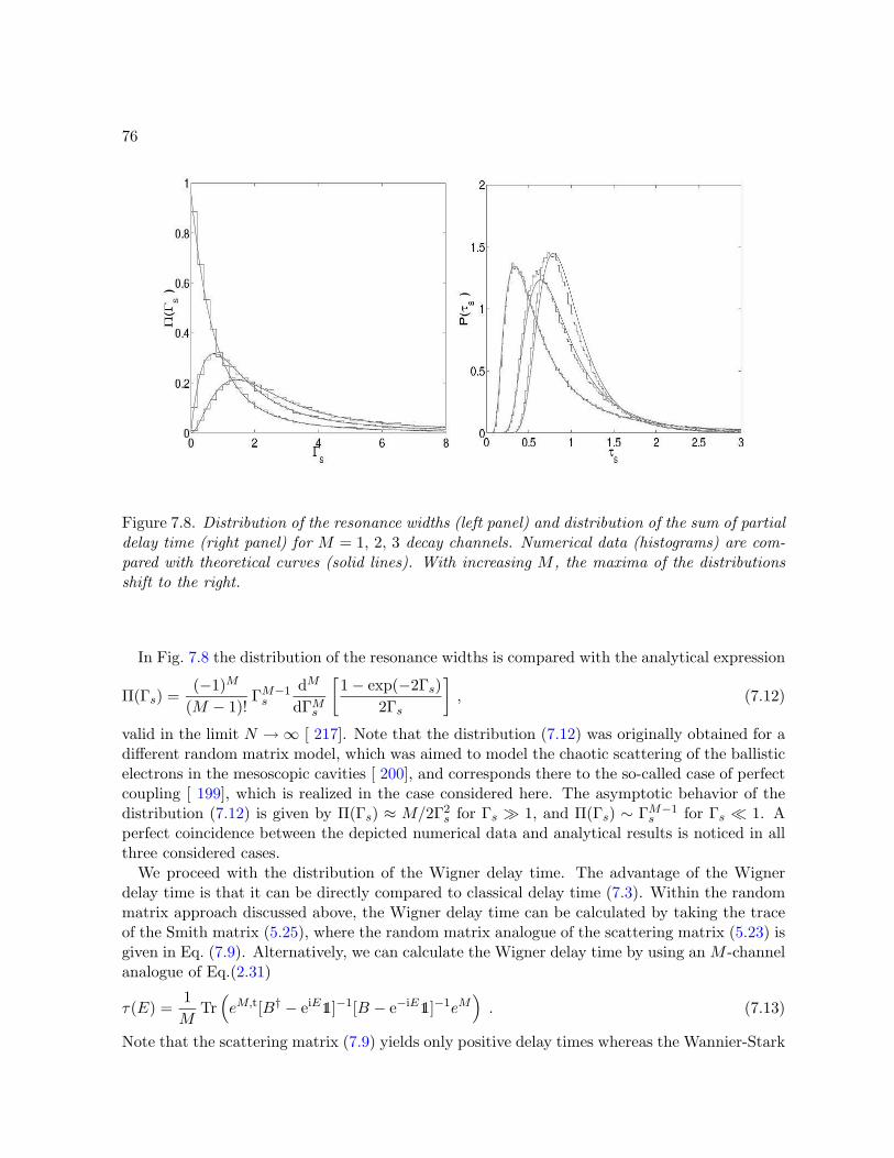
76

Figure 7.8. Distribution of the resonance widths (left panel) and distribution of the sum of partialdelay time (right panel) for M = 1, 2, 3 decay channels. Numerical data (histograms) are com-pared with theoretical curves (solid lines). With increasing M , the maxima of the distributionsshift to the right.

In Fig. 7.8 the distribution of the resonance widths is compared with the analytical expression

Π(Γs) =(−1)M

(M − 1)!ΓM−1s

dM

dΓMs

[1− exp(−2Γs)

2Γs

], (7.12)

valid in the limit N →∞ [ 217]. Note that the distribution (7.12) was originally obtained for adifferent random matrix model, which was aimed to model the chaotic scattering of the ballisticelectrons in the mesoscopic cavities [ 200], and corresponds there to the so-called case of perfectcoupling [ 199], which is realized in the case considered here. The asymptotic behavior of thedistribution (7.12) is given by Π(Γs) ≈ M/2Γ2

s for Γs 1, and Π(Γs) ∼ ΓM−1s for Γs 1. A

perfect coincidence between the depicted numerical data and analytical results is noticed in allthree considered cases.

We proceed with the distribution of the Wigner delay time. The advantage of the Wignerdelay time is that it can be directly compared to classical delay time (7.3). Within the randommatrix approach discussed above, the Wigner delay time can be calculated by taking the traceof the Smith matrix (5.25), where the random matrix analogue of the scattering matrix (5.23) isgiven in Eq. (7.9). Alternatively, we can calculate the Wigner delay time by using an M -channelanalogue of Eq.(2.31)

τ(E) =1M

Tr(eM,t[B† − eiE11]−1[B − e−iE11]−1eM

). (7.13)

Note that the scattering matrix (7.9) yields only positive delay times whereas the Wannier-Stark

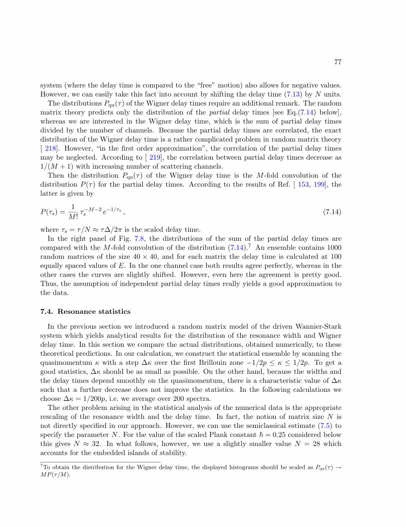
77

system (where the delay time is compared to the “free” motion) also allows for negative values.However, we can easily take this fact into account by shifting the delay time (7.13) by N units.

The distributions Pqu(τ) of the Wigner delay times require an additional remark. The randommatrix theory predicts only the distribution of the partial delay times [see Eq.(7.14) below],whereas we are interested in the Wigner delay time, which is the sum of partial delay timesdivided by the number of channels. Because the partial delay times are correlated, the exactdistribution of the Wigner delay time is a rather complicated problem in random matrix theory[ 218]. However, “in the first order approximation”, the correlation of the partial delay timesmay be neglected. According to [ 219], the correlation between partial delay times decrease as1/(M + 1) with increasing number of scattering channels.

Then the distribution Pqu(τ) of the Wigner delay time is the M -fold convolution of thedistribution P (τ) for the partial delay times. According to the results of Ref. [ 153, 199], thelatter is given by

P (τs) =1M !

τ−M−2s e−1/τs , (7.14)

where τs = τ/N ≈ τ∆/2π is the scaled delay time.In the right panel of Fig. 7.8, the distributions of the sum of the partial delay times are

compared with the M -fold convolution of the distribution (7.14).7 An ensemble contains 1000random matrices of the size 40 × 40, and for each matrix the delay time is calculated at 100equally spaced values of E. In the one channel case both results agree perfectly, whereas in theother cases the curves are slightly shifted. However, even here the agreement is pretty good.Thus, the assumption of independent partial delay times really yields a good approximation tothe data.

7.4. Resonance statistics

In the previous section we introduced a random matrix model of the driven Wannier-Starksystem which yields analytical results for the distribution of the resonance width and Wignerdelay time. In this section we compare the actual distributions, obtained numerically, to thesetheoretical predictions. In our calculation, we construct the statistical ensemble by scanning thequasimomentum κ with a step ∆κ over the first Brillouin zone −1/2p ≤ κ ≤ 1/2p. To get agood statistics, ∆κ should be as small as possible. On the other hand, because the widths andthe delay times depend smoothly on the quasimomentum, there is a characteristic value of ∆κsuch that a further decrease does not improve the statistics. In the following calculations wechoose ∆κ = 1/200p, i.e. we average over 200 spectra.

The other problem arising in the statistical analysis of the numerical data is the appropriaterescaling of the resonance width and the delay time. In fact, the notion of matrix size N isnot directly specified in our approach. However, we can use the semiclassical estimate (7.5) tospecify the parameter N . For the value of the scaled Plank constant ~ = 0.25 considered belowthis gives N ≈ 32. In what follows, however, we use a slightly smaller value N = 28 whichaccounts for the embedded islands of stability.

7To obtain the distribution for the Wigner delay time, the displayed histograms should be scaled as Pqu(τ) →MP (τ/M).

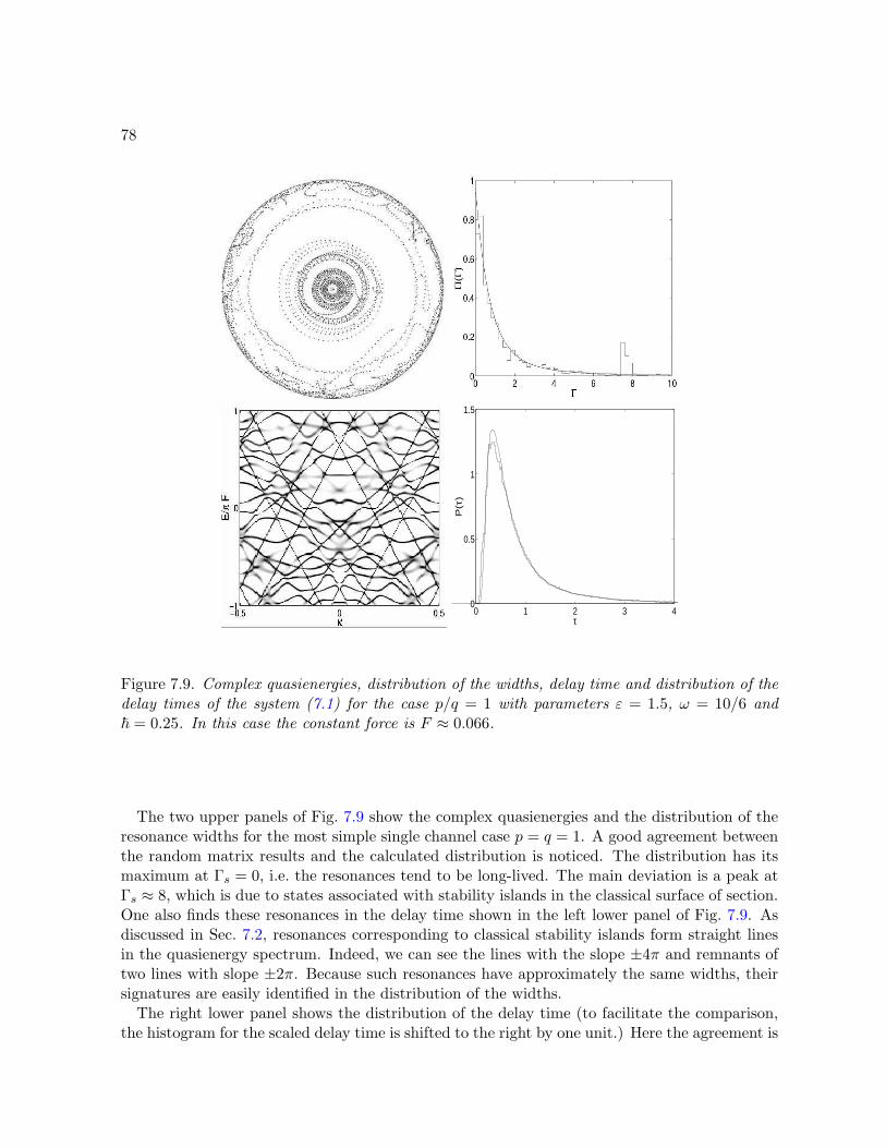
78

0 1 2 3 40

0.5

1

1.5

τ

P(τ

)

Figure 7.9. Complex quasienergies, distribution of the widths, delay time and distribution of thedelay times of the system (7.1) for the case p/q = 1 with parameters ε = 1.5, ω = 10/6 and~ = 0.25. In this case the constant force is F ≈ 0.066.

The two upper panels of Fig. 7.9 show the complex quasienergies and the distribution of theresonance widths for the most simple single channel case p = q = 1. A good agreement betweenthe random matrix results and the calculated distribution is noticed. The distribution has itsmaximum at Γs = 0, i.e. the resonances tend to be long-lived. The main deviation is a peak atΓs ≈ 8, which is due to states associated with stability islands in the classical surface of section.One also finds these resonances in the delay time shown in the left lower panel of Fig. 7.9. Asdiscussed in Sec. 7.2, resonances corresponding to classical stability islands form straight linesin the quasienergy spectrum. Indeed, we can see the lines with the slope ±4π and remnants oftwo lines with slope ±2π. Because such resonances have approximately the same widths, theirsignatures are easily identified in the distribution of the widths.

The right lower panel shows the distribution of the delay time (to facilitate the comparison,the histogram for the scaled delay time is shifted to the right by one unit.) Here the agreement is

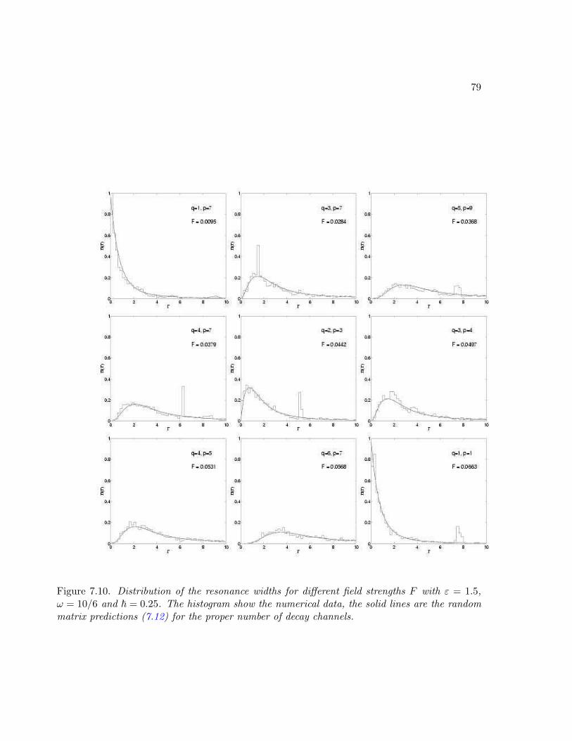
79

Figure 7.10. Distribution of the resonance widths for different field strengths F with ε = 1.5,ω = 10/6 and ~ = 0.25. The histogram show the numerical data, the solid lines are the randommatrix predictions (7.12) for the proper number of decay channels.

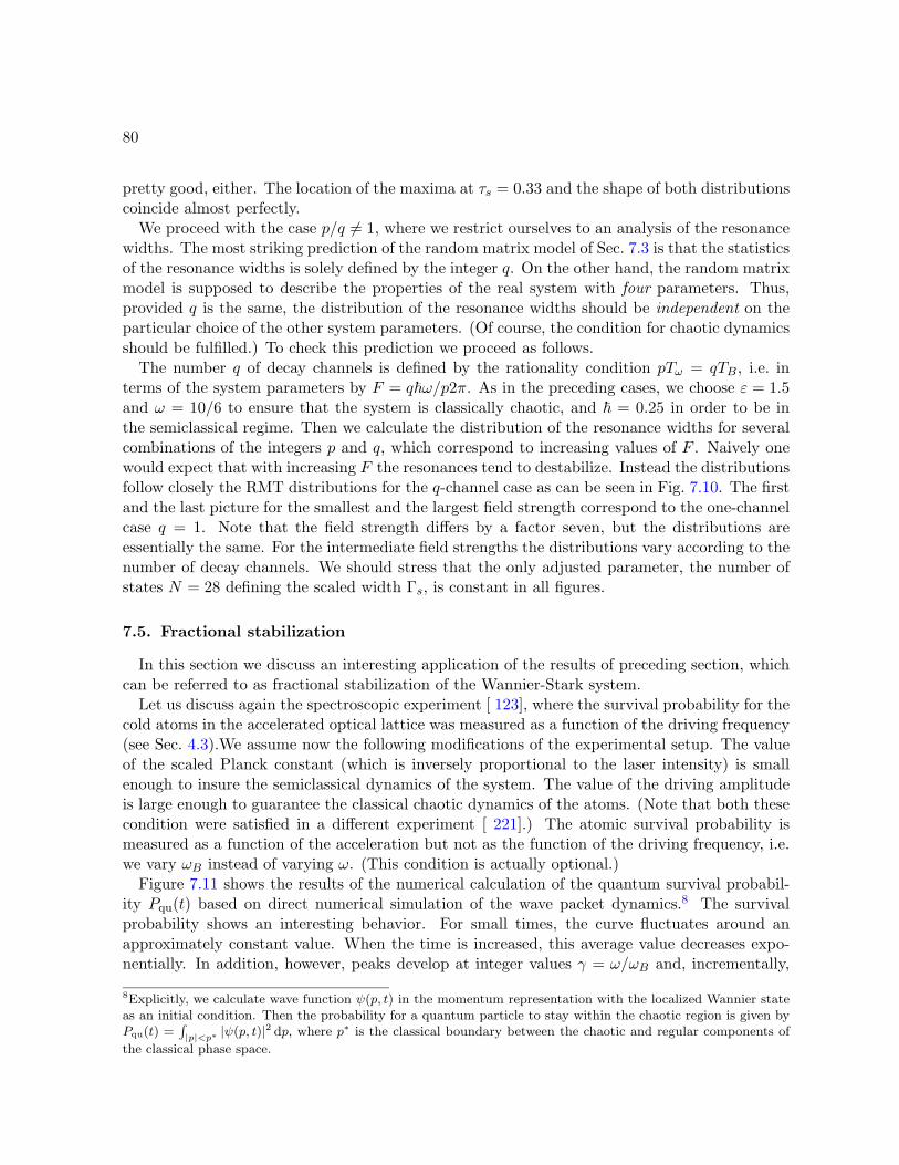
80

pretty good, either. The location of the maxima at τs = 0.33 and the shape of both distributionscoincide almost perfectly.

We proceed with the case p/q 6= 1, where we restrict ourselves to an analysis of the resonancewidths. The most striking prediction of the random matrix model of Sec. 7.3 is that the statisticsof the resonance widths is solely defined by the integer q. On the other hand, the random matrixmodel is supposed to describe the properties of the real system with four parameters. Thus,provided q is the same, the distribution of the resonance widths should be independent on theparticular choice of the other system parameters. (Of course, the condition for chaotic dynamicsshould be fulfilled.) To check this prediction we proceed as follows.

The number q of decay channels is defined by the rationality condition pTω = qTB, i.e. interms of the system parameters by F = q~ω/p2π. As in the preceding cases, we choose ε = 1.5and ω = 10/6 to ensure that the system is classically chaotic, and ~ = 0.25 in order to be inthe semiclassical regime. Then we calculate the distribution of the resonance widths for severalcombinations of the integers p and q, which correspond to increasing values of F . Naively onewould expect that with increasing F the resonances tend to destabilize. Instead the distributionsfollow closely the RMT distributions for the q-channel case as can be seen in Fig. 7.10. The firstand the last picture for the smallest and the largest field strength correspond to the one-channelcase q = 1. Note that the field strength differs by a factor seven, but the distributions areessentially the same. For the intermediate field strengths the distributions vary according to thenumber of decay channels. We should stress that the only adjusted parameter, the number ofstates N = 28 defining the scaled width Γs, is constant in all figures.

7.5. Fractional stabilization

In this section we discuss an interesting application of the results of preceding section, whichcan be referred to as fractional stabilization of the Wannier-Stark system.

Let us discuss again the spectroscopic experiment [ 123], where the survival probability for thecold atoms in the accelerated optical lattice was measured as a function of the driving frequency(see Sec. 4.3).We assume now the following modifications of the experimental setup. The valueof the scaled Planck constant (which is inversely proportional to the laser intensity) is smallenough to insure the semiclassical dynamics of the system. The value of the driving amplitudeis large enough to guarantee the classical chaotic dynamics of the atoms. (Note that both thesecondition were satisfied in a different experiment [ 221].) The atomic survival probability ismeasured as a function of the acceleration but not as the function of the driving frequency, i.e.we vary ωB instead of varying ω. (This condition is actually optional.)

Figure 7.11 shows the results of the numerical calculation of the quantum survival probabil-ity Pqu(t) based on direct numerical simulation of the wave packet dynamics.8 The survivalprobability shows an interesting behavior. For small times, the curve fluctuates around anapproximately constant value. When the time is increased, this average value decreases expo-nentially. In addition, however, peaks develop at integer values γ = ω/ωB and, incrementally,

8Explicitly, we calculate wave function ψ(p, t) in the momentum representation with the localized Wannier stateas an initial condition. Then the probability for a quantum particle to stay within the chaotic region is given byPqu(t) =

∫|p|<p∗ |ψ(p, t)|2 dp, where p∗ is the classical boundary between the chaotic and regular components of

the classical phase space.

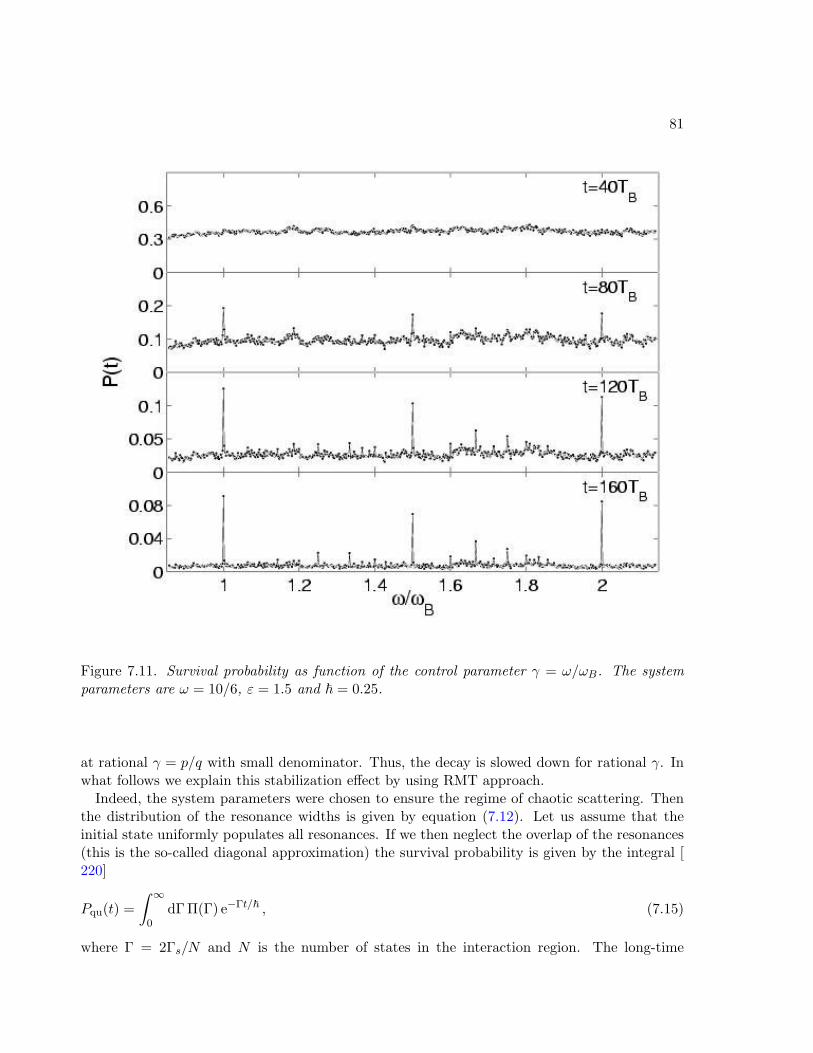
81

Figure 7.11. Survival probability as function of the control parameter γ = ω/ωB. The systemparameters are ω = 10/6, ε = 1.5 and ~ = 0.25.

at rational γ = p/q with small denominator. Thus, the decay is slowed down for rational γ. Inwhat follows we explain this stabilization effect by using RMT approach.

Indeed, the system parameters were chosen to ensure the regime of chaotic scattering. Thenthe distribution of the resonance widths is given by equation (7.12). Let us assume that theinitial state uniformly populates all resonances. If we then neglect the overlap of the resonances(this is the so-called diagonal approximation) the survival probability is given by the integral [220]

Pqu(t) =∫ ∞

0dΓ Π(Γ) e−Γt/~ , (7.15)

where Γ = 2Γs/N and N is the number of states in the interaction region. The long-time

82

Figure 7.12. Survival probability at t = 200TB. The left part shows the numerical data, the rightpart the theoretical curve based on equation (7.16). To stress the discontinuous character of thelatter function, we slightly changed its graphical representation.

asymptotics of this integral is defined by the behavior of Π(Γ) at small Γ, where it increases asthe power law Π(Γ) ∼ Γq−1. Consequently, the survival probability asymptotically follows theinverse power law Pqu(t) ∼ t−q. Thus, the asymptotics depend on the number of decay channelsand therefore on the denominator of the control parameter γ = ω/ωB = p/q.

With the help of supersymmetric techniques, Pqu(t) can be calculated beyond the diagonalapproximation. This gives more elaborated result [ 220]

Pqu(t) ≈(

1 +ΓW t~q

)−q. (7.16)

where ΓW is the so-called Weisskopf width (which is a free parameter in the abstract ran-dom matrix theory). For rational γ and large times the decay of the survival probability isalgebraic, Pqu(t) ∼ t−q, as found in the diagonal approximation. The case of irrational γcan be approximated by the limit q → ∞. Then the system shows the exponential decay,Pqu(t) = exp(−ΓW t/~) and its natural to identify the parameter ΓW /~ with the classical decaycoefficient ν.

The right panel in Fig. 7.12 shows the values of the function (7.16) for t = 200TB and somerational values of γ = ω/ωB. Here we use a slightly different graphic presentation of Pqu(t) tostress that the function (7.16) is a discontinuous function of γ for any t. In contrast, the atomicsurvival probability shown in the left panel is a continuous function of γ where its discontinuousstructure develops gradually as t → ∞. In fact, the survival probabilities calculated for two

83

close rational numbers γ1 and γ2 follow each other during a finite “correspondence” time. (Forinstance, for γ1 = 1 and γ2 = 999/1000 the correspondence time is found to be about 50TB.)Thus it takes some time to distinguish two close rationals, although they may have very differentdenominators and, therefore, very different asymptotics. With this remark reserved, a nicestructural (and even semiquantitative) correspondence is noticed.

The described numerical experiment suggest a simple laboratory experiment with cold atomsin optical lattice, where one can test the statistics of the resonance width indirectly, by measuringthe survival probability for atoms.

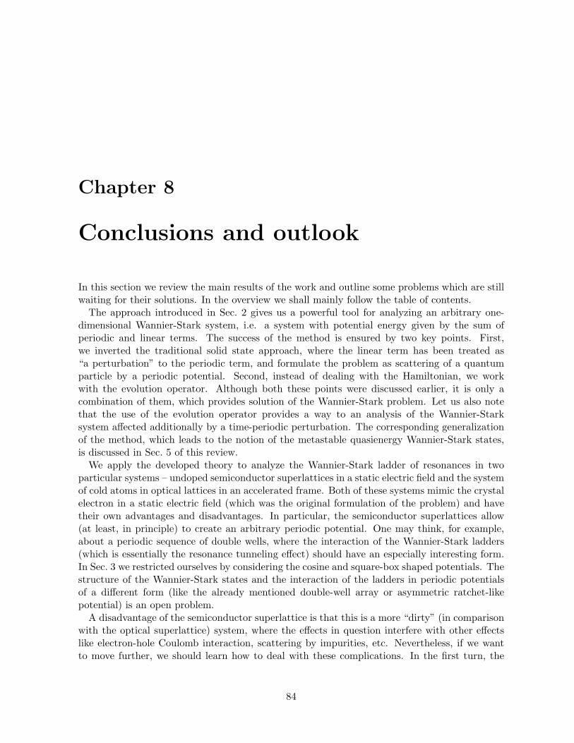
Chapter 8

Conclusions and outlook

In this section we review the main results of the work and outline some problems which are stillwaiting for their solutions. In the overview we shall mainly follow the table of contents.

The approach introduced in Sec. 2 gives us a powerful tool for analyzing an arbitrary one-dimensional Wannier-Stark system, i.e. a system with potential energy given by the sum ofperiodic and linear terms. The success of the method is ensured by two key points. First,we inverted the traditional solid state approach, where the linear term has been treated as“a perturbation” to the periodic term, and formulate the problem as scattering of a quantumparticle by a periodic potential. Second, instead of dealing with the Hamiltonian, we workwith the evolution operator. Although both these points were discussed earlier, it is only acombination of them, which provides solution of the Wannier-Stark problem. Let us also notethat the use of the evolution operator provides a way to an analysis of the Wannier-Starksystem affected additionally by a time-periodic perturbation. The corresponding generalizationof the method, which leads to the notion of the metastable quasienergy Wannier-Stark states,is discussed in Sec. 5 of this review.

We apply the developed theory to analyze the Wannier-Stark ladder of resonances in twoparticular systems – undoped semiconductor superlattices in a static electric field and the systemof cold atoms in optical lattices in an accelerated frame. Both of these systems mimic the crystalelectron in a static electric field (which was the original formulation of the problem) and havetheir own advantages and disadvantages. In particular, the semiconductor superlattices allow(at least, in principle) to create an arbitrary periodic potential. One may think, for example,about a periodic sequence of double wells, where the interaction of the Wannier-Stark ladders(which is essentially the resonance tunneling effect) should have an especially interesting form.In Sec. 3 we restricted ourselves by considering the cosine and square-box shaped potentials. Thestructure of the Wannier-Stark states and the interaction of the ladders in periodic potentialsof a different form (like the already mentioned double-well array or asymmetric ratchet-likepotential) is an open problem.

A disadvantage of the semiconductor superlattice is that this is a more “dirty” (in comparisonwith the optical superlattice) system, where the effects in question interfere with other effectslike electron-hole Coulomb interaction, scattering by impurities, etc. Nevertheless, if we wantto move further, we should learn how to deal with these complications. In the first turn, the

84

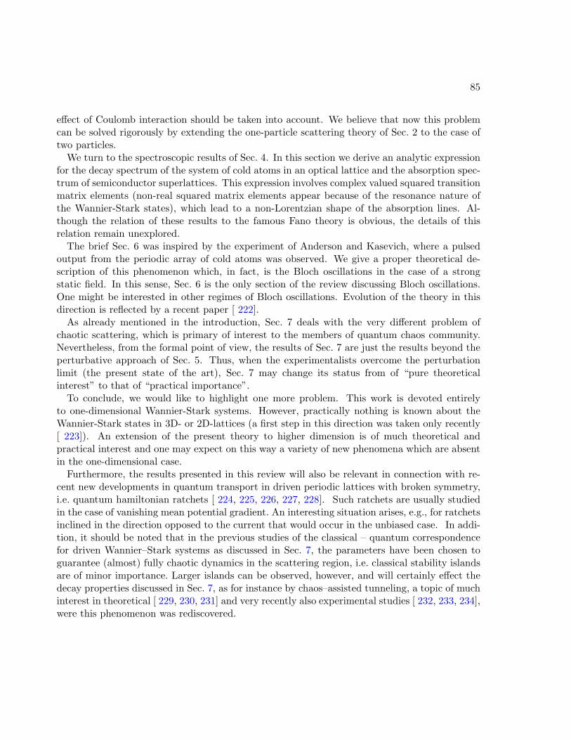
85

effect of Coulomb interaction should be taken into account. We believe that now this problemcan be solved rigorously by extending the one-particle scattering theory of Sec. 2 to the case oftwo particles.

We turn to the spectroscopic results of Sec. 4. In this section we derive an analytic expressionfor the decay spectrum of the system of cold atoms in an optical lattice and the absorption spec-trum of semiconductor superlattices. This expression involves complex valued squared transitionmatrix elements (non-real squared matrix elements appear because of the resonance nature ofthe Wannier-Stark states), which lead to a non-Lorentzian shape of the absorption lines. Al-though the relation of these results to the famous Fano theory is obvious, the details of thisrelation remain unexplored.

The brief Sec. 6 was inspired by the experiment of Anderson and Kasevich, where a pulsedoutput from the periodic array of cold atoms was observed. We give a proper theoretical de-scription of this phenomenon which, in fact, is the Bloch oscillations in the case of a strongstatic field. In this sense, Sec. 6 is the only section of the review discussing Bloch oscillations.One might be interested in other regimes of Bloch oscillations. Evolution of the theory in thisdirection is reflected by a recent paper [ 222].

As already mentioned in the introduction, Sec. 7 deals with the very different problem ofchaotic scattering, which is primary of interest to the members of quantum chaos community.Nevertheless, from the formal point of view, the results of Sec. 7 are just the results beyond theperturbative approach of Sec. 5. Thus, when the experimentalists overcome the perturbationlimit (the present state of the art), Sec. 7 may change its status from of “pure theoreticalinterest” to that of “practical importance”.

To conclude, we would like to highlight one more problem. This work is devoted entirelyto one-dimensional Wannier-Stark systems. However, practically nothing is known about theWannier-Stark states in 3D- or 2D-lattices (a first step in this direction was taken only recently[ 223]). An extension of the present theory to higher dimension is of much theoretical andpractical interest and one may expect on this way a variety of new phenomena which are absentin the one-dimensional case.

Furthermore, the results presented in this review will also be relevant in connection with re-cent new developments in quantum transport in driven periodic lattices with broken symmetry,i.e. quantum hamiltonian ratchets [ 224, 225, 226, 227, 228]. Such ratchets are usually studiedin the case of vanishing mean potential gradient. An interesting situation arises, e.g., for ratchetsinclined in the direction opposed to the current that would occur in the unbiased case. In addi-tion, it should be noted that in the previous studies of the classical – quantum correspondencefor driven Wannier–Stark systems as discussed in Sec. 7, the parameters have been chosen toguarantee (almost) fully chaotic dynamics in the scattering region, i.e. classical stability islandsare of minor importance. Larger islands can be observed, however, and will certainly effect thedecay properties discussed in Sec. 7, as for instance by chaos–assisted tunneling, a topic of muchinterest in theoretical [ 229, 230, 231] and very recently also experimental studies [ 232, 233, 234],were this phenomenon was rediscovered.

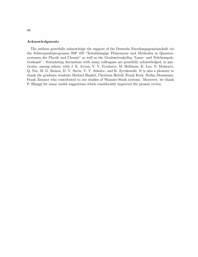
86

Acknowledgments

The authors gratefully acknowledge the support of the Deutsche Forschungsgemeinschaft viathe Schwerpunktprogramm SSP 470 “Zeitabhangige Phanomene und Methoden in Quanten-systemen der Physik und Chemie” as well as the Graduiertenkolleg “Laser- und Teilchenspek-troskopie”. Stimulating discussions with many colleagues are gratefully acknowledged, in par-ticular, among others, with J. E. Avron, Y. V. Fyodorov, M. Holthaus, K. Leo, N. Moiseyev,Q. Niu, M. G. Raizen, D. V. Savin, V. V. Sokolov, and K. Zyczkowski. It is also a pleasure tothank the graduate students Michael Hankel, Christian Hebell, Frank Keck, Stefan Mossmann,Frank Zimmer who contributed to our studies of Wannier-Stark systems. Moreover, we thankP. Hanggi for many useful suggestions which considerably improved the present review.

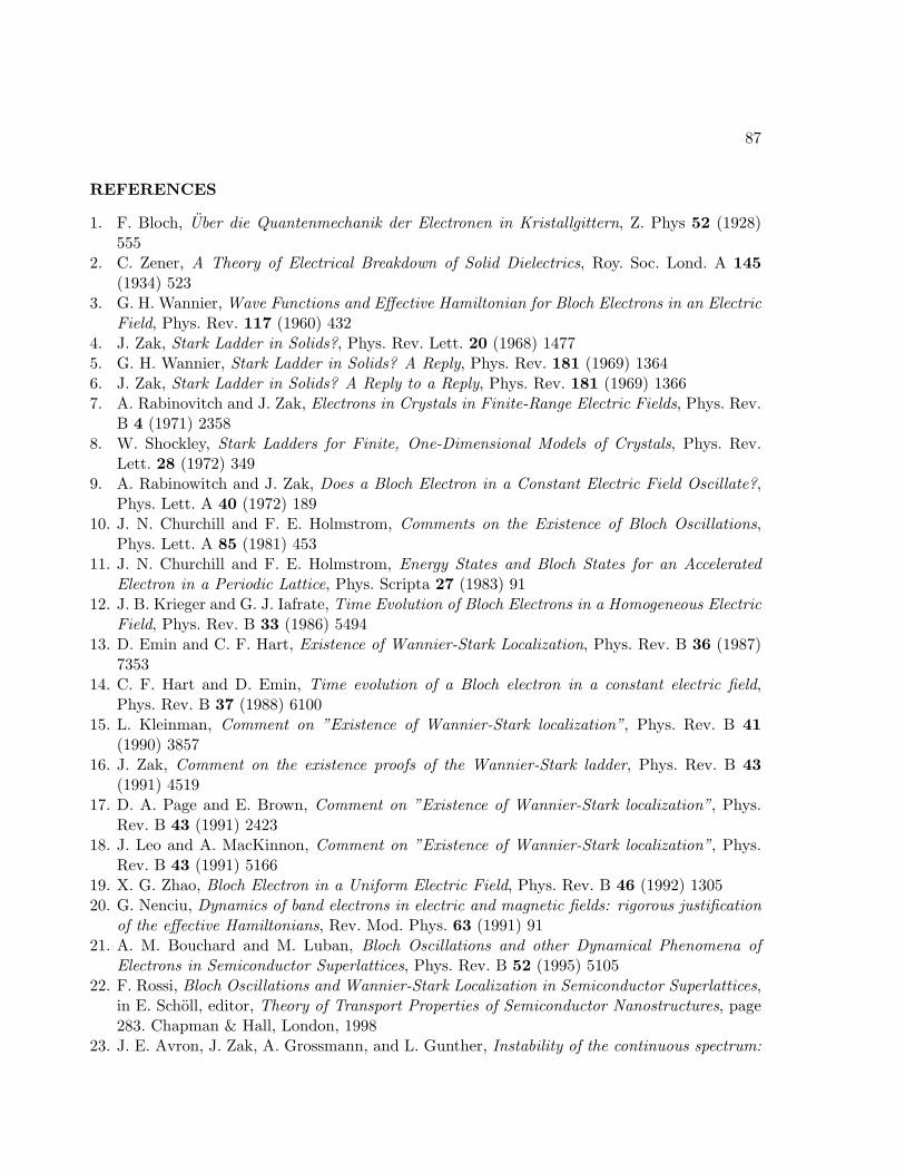
87

REFERENCES

1. F. Bloch, Uber die Quantenmechanik der Electronen in Kristallgittern, Z. Phys 52 (1928)555

2. C. Zener, A Theory of Electrical Breakdown of Solid Dielectrics, Roy. Soc. Lond. A 145(1934) 523

3. G. H. Wannier, Wave Functions and Effective Hamiltonian for Bloch Electrons in an ElectricField, Phys. Rev. 117 (1960) 432

4. J. Zak, Stark Ladder in Solids?, Phys. Rev. Lett. 20 (1968) 14775. G. H. Wannier, Stark Ladder in Solids? A Reply, Phys. Rev. 181 (1969) 13646. J. Zak, Stark Ladder in Solids? A Reply to a Reply, Phys. Rev. 181 (1969) 13667. A. Rabinovitch and J. Zak, Electrons in Crystals in Finite-Range Electric Fields, Phys. Rev.

B 4 (1971) 23588. W. Shockley, Stark Ladders for Finite, One-Dimensional Models of Crystals, Phys. Rev.

Lett. 28 (1972) 3499. A. Rabinowitch and J. Zak, Does a Bloch Electron in a Constant Electric Field Oscillate?,

Phys. Lett. A 40 (1972) 18910. J. N. Churchill and F. E. Holmstrom, Comments on the Existence of Bloch Oscillations,

Phys. Lett. A 85 (1981) 45311. J. N. Churchill and F. E. Holmstrom, Energy States and Bloch States for an Accelerated

Electron in a Periodic Lattice, Phys. Scripta 27 (1983) 9112. J. B. Krieger and G. J. Iafrate, Time Evolution of Bloch Electrons in a Homogeneous Electric

Field, Phys. Rev. B 33 (1986) 549413. D. Emin and C. F. Hart, Existence of Wannier-Stark Localization, Phys. Rev. B 36 (1987)

735314. C. F. Hart and D. Emin, Time evolution of a Bloch electron in a constant electric field,

Phys. Rev. B 37 (1988) 610015. L. Kleinman, Comment on ”Existence of Wannier-Stark localization”, Phys. Rev. B 41

(1990) 385716. J. Zak, Comment on the existence proofs of the Wannier-Stark ladder, Phys. Rev. B 43

(1991) 451917. D. A. Page and E. Brown, Comment on ”Existence of Wannier-Stark localization”, Phys.

Rev. B 43 (1991) 242318. J. Leo and A. MacKinnon, Comment on ”Existence of Wannier-Stark localization”, Phys.

Rev. B 43 (1991) 516619. X. G. Zhao, Bloch Electron in a Uniform Electric Field, Phys. Rev. B 46 (1992) 130520. G. Nenciu, Dynamics of band electrons in electric and magnetic fields: rigorous justification

of the effective Hamiltonians, Rev. Mod. Phys. 63 (1991) 9121. A. M. Bouchard and M. Luban, Bloch Oscillations and other Dynamical Phenomena of

Electrons in Semiconductor Superlattices, Phys. Rev. B 52 (1995) 510522. F. Rossi, Bloch Oscillations and Wannier-Stark Localization in Semiconductor Superlattices,

in E. Scholl, editor, Theory of Transport Properties of Semiconductor Nanostructures, page283. Chapman & Hall, London, 1998

23. J. E. Avron, J. Zak, A. Grossmann, and L. Gunther, Instability of the continuous spectrum:

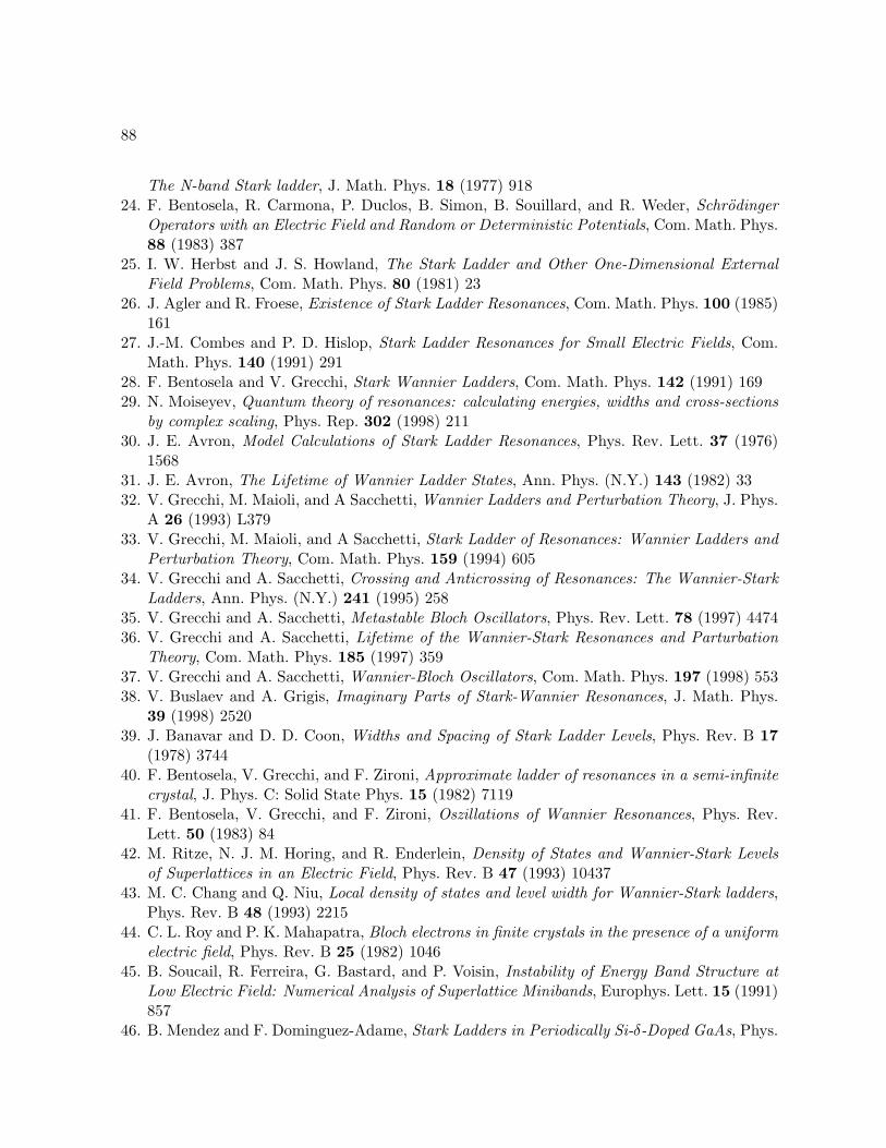
88

The N-band Stark ladder, J. Math. Phys. 18 (1977) 91824. F. Bentosela, R. Carmona, P. Duclos, B. Simon, B. Souillard, and R. Weder, Schrodinger

Operators with an Electric Field and Random or Deterministic Potentials, Com. Math. Phys.88 (1983) 387

25. I. W. Herbst and J. S. Howland, The Stark Ladder and Other One-Dimensional ExternalField Problems, Com. Math. Phys. 80 (1981) 23

26. J. Agler and R. Froese, Existence of Stark Ladder Resonances, Com. Math. Phys. 100 (1985)161

27. J.-M. Combes and P. D. Hislop, Stark Ladder Resonances for Small Electric Fields, Com.Math. Phys. 140 (1991) 291

28. F. Bentosela and V. Grecchi, Stark Wannier Ladders, Com. Math. Phys. 142 (1991) 16929. N. Moiseyev, Quantum theory of resonances: calculating energies, widths and cross-sections

by complex scaling, Phys. Rep. 302 (1998) 21130. J. E. Avron, Model Calculations of Stark Ladder Resonances, Phys. Rev. Lett. 37 (1976)

156831. J. E. Avron, The Lifetime of Wannier Ladder States, Ann. Phys. (N.Y.) 143 (1982) 3332. V. Grecchi, M. Maioli, and A Sacchetti, Wannier Ladders and Perturbation Theory, J. Phys.

A 26 (1993) L37933. V. Grecchi, M. Maioli, and A Sacchetti, Stark Ladder of Resonances: Wannier Ladders and

Perturbation Theory, Com. Math. Phys. 159 (1994) 60534. V. Grecchi and A. Sacchetti, Crossing and Anticrossing of Resonances: The Wannier-Stark

Ladders, Ann. Phys. (N.Y.) 241 (1995) 25835. V. Grecchi and A. Sacchetti, Metastable Bloch Oscillators, Phys. Rev. Lett. 78 (1997) 447436. V. Grecchi and A. Sacchetti, Lifetime of the Wannier-Stark Resonances and Parturbation

Theory, Com. Math. Phys. 185 (1997) 35937. V. Grecchi and A. Sacchetti, Wannier-Bloch Oscillators, Com. Math. Phys. 197 (1998) 55338. V. Buslaev and A. Grigis, Imaginary Parts of Stark-Wannier Resonances, J. Math. Phys.

39 (1998) 252039. J. Banavar and D. D. Coon, Widths and Spacing of Stark Ladder Levels, Phys. Rev. B 17

(1978) 374440. F. Bentosela, V. Grecchi, and F. Zironi, Approximate ladder of resonances in a semi-infinite

crystal, J. Phys. C: Solid State Phys. 15 (1982) 711941. F. Bentosela, V. Grecchi, and F. Zironi, Oszillations of Wannier Resonances, Phys. Rev.

Lett. 50 (1983) 8442. M. Ritze, N. J. M. Horing, and R. Enderlein, Density of States and Wannier-Stark Levels

of Superlattices in an Electric Field, Phys. Rev. B 47 (1993) 1043743. M. C. Chang and Q. Niu, Local density of states and level width for Wannier-Stark ladders,

Phys. Rev. B 48 (1993) 221544. C. L. Roy and P. K. Mahapatra, Bloch electrons in finite crystals in the presence of a uniform

electric field, Phys. Rev. B 25 (1982) 104645. B. Soucail, R. Ferreira, G. Bastard, and P. Voisin, Instability of Energy Band Structure at

Low Electric Field: Numerical Analysis of Superlattice Minibands, Europhys. Lett. 15 (1991)857

46. B. Mendez and F. Dominguez-Adame, Stark Ladders in Periodically Si-δ-Doped GaAs, Phys.

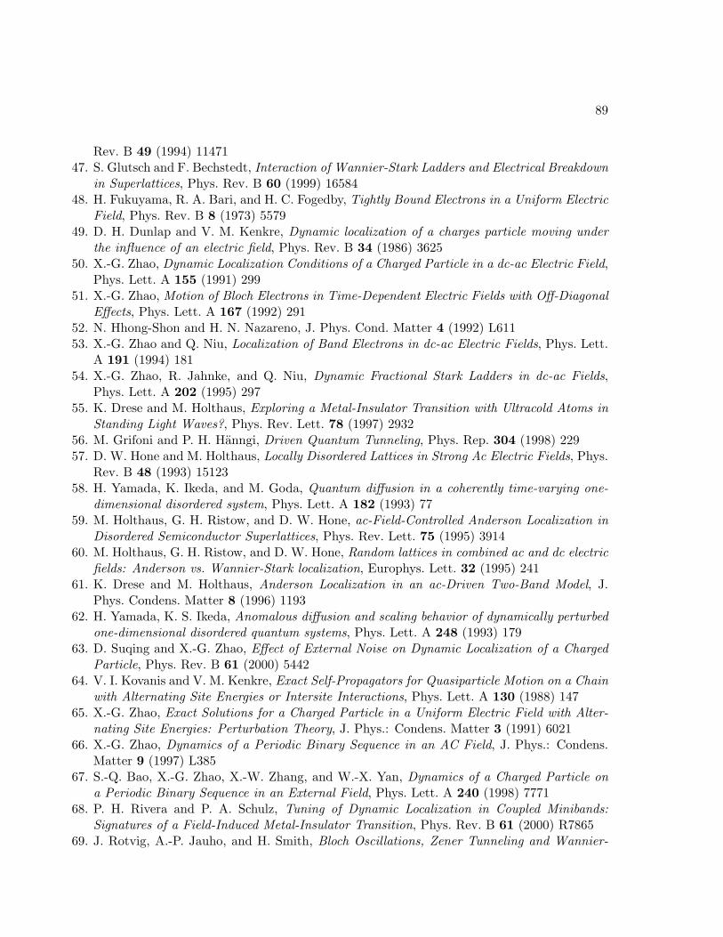
89

Rev. B 49 (1994) 1147147. S. Glutsch and F. Bechstedt, Interaction of Wannier-Stark Ladders and Electrical Breakdown

in Superlattices, Phys. Rev. B 60 (1999) 1658448. H. Fukuyama, R. A. Bari, and H. C. Fogedby, Tightly Bound Electrons in a Uniform Electric

Field, Phys. Rev. B 8 (1973) 557949. D. H. Dunlap and V. M. Kenkre, Dynamic localization of a charges particle moving under

the influence of an electric field, Phys. Rev. B 34 (1986) 362550. X.-G. Zhao, Dynamic Localization Conditions of a Charged Particle in a dc-ac Electric Field,

Phys. Lett. A 155 (1991) 29951. X.-G. Zhao, Motion of Bloch Electrons in Time-Dependent Electric Fields with Off-Diagonal

Effects, Phys. Lett. A 167 (1992) 29152. N. Hhong-Shon and H. N. Nazareno, J. Phys. Cond. Matter 4 (1992) L61153. X.-G. Zhao and Q. Niu, Localization of Band Electrons in dc-ac Electric Fields, Phys. Lett.

A 191 (1994) 18154. X.-G. Zhao, R. Jahnke, and Q. Niu, Dynamic Fractional Stark Ladders in dc-ac Fields,

Phys. Lett. A 202 (1995) 29755. K. Drese and M. Holthaus, Exploring a Metal-Insulator Transition with Ultracold Atoms in

Standing Light Waves?, Phys. Rev. Lett. 78 (1997) 293256. M. Grifoni and P. H. Hanngi, Driven Quantum Tunneling, Phys. Rep. 304 (1998) 22957. D. W. Hone and M. Holthaus, Locally Disordered Lattices in Strong Ac Electric Fields, Phys.

Rev. B 48 (1993) 1512358. H. Yamada, K. Ikeda, and M. Goda, Quantum diffusion in a coherently time-varying one-

dimensional disordered system, Phys. Lett. A 182 (1993) 7759. M. Holthaus, G. H. Ristow, and D. W. Hone, ac-Field-Controlled Anderson Localization in

Disordered Semiconductor Superlattices, Phys. Rev. Lett. 75 (1995) 391460. M. Holthaus, G. H. Ristow, and D. W. Hone, Random lattices in combined ac and dc electric

fields: Anderson vs. Wannier-Stark localization, Europhys. Lett. 32 (1995) 24161. K. Drese and M. Holthaus, Anderson Localization in an ac-Driven Two-Band Model, J.

Phys. Condens. Matter 8 (1996) 119362. H. Yamada, K. S. Ikeda, Anomalous diffusion and scaling behavior of dynamically perturbed

one-dimensional disordered quantum systems, Phys. Lett. A 248 (1993) 17963. D. Suqing and X.-G. Zhao, Effect of External Noise on Dynamic Localization of a Charged

Particle, Phys. Rev. B 61 (2000) 544264. V. I. Kovanis and V. M. Kenkre, Exact Self-Propagators for Quasiparticle Motion on a Chain

with Alternating Site Energies or Intersite Interactions, Phys. Lett. A 130 (1988) 14765. X.-G. Zhao, Exact Solutions for a Charged Particle in a Uniform Electric Field with Alter-

nating Site Energies: Perturbation Theory, J. Phys.: Condens. Matter 3 (1991) 602166. X.-G. Zhao, Dynamics of a Periodic Binary Sequence in an AC Field, J. Phys.: Condens.

Matter 9 (1997) L38567. S.-Q. Bao, X.-G. Zhao, X.-W. Zhang, and W.-X. Yan, Dynamics of a Charged Particle on

a Periodic Binary Sequence in an External Field, Phys. Lett. A 240 (1998) 777168. P. H. Rivera and P. A. Schulz, Tuning of Dynamic Localization in Coupled Minibands:

Signatures of a Field-Induced Metal-Insulator Transition, Phys. Rev. B 61 (2000) R786569. J. Rotvig, A.-P. Jauho, and H. Smith, Bloch Oscillations, Zener Tunneling and Wannier-

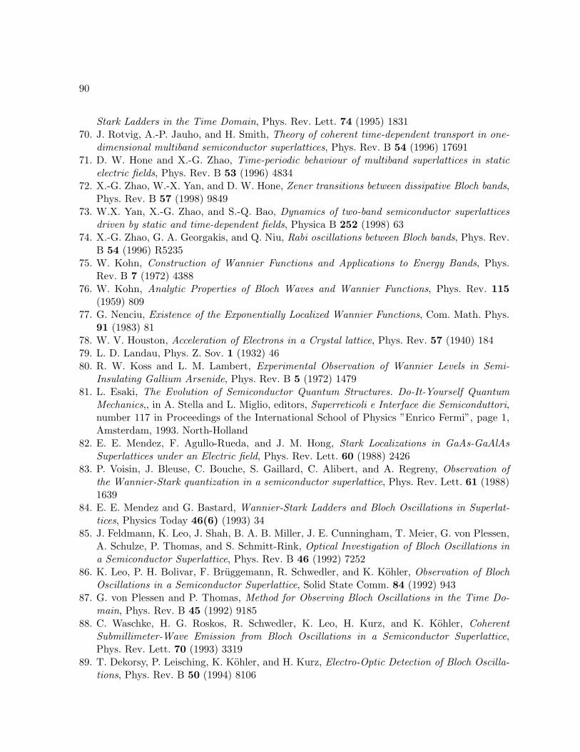
90

Stark Ladders in the Time Domain, Phys. Rev. Lett. 74 (1995) 183170. J. Rotvig, A.-P. Jauho, and H. Smith, Theory of coherent time-dependent transport in one-

dimensional multiband semiconductor superlattices, Phys. Rev. B 54 (1996) 1769171. D. W. Hone and X.-G. Zhao, Time-periodic behaviour of multiband superlattices in static

electric fields, Phys. Rev. B 53 (1996) 483472. X.-G. Zhao, W.-X. Yan, and D. W. Hone, Zener transitions between dissipative Bloch bands,

Phys. Rev. B 57 (1998) 984973. W.X. Yan, X.-G. Zhao, and S.-Q. Bao, Dynamics of two-band semiconductor superlattices

driven by static and time-dependent fields, Physica B 252 (1998) 6374. X.-G. Zhao, G. A. Georgakis, and Q. Niu, Rabi oscillations between Bloch bands, Phys. Rev.

B 54 (1996) R523575. W. Kohn, Construction of Wannier Functions and Applications to Energy Bands, Phys.

Rev. B 7 (1972) 438876. W. Kohn, Analytic Properties of Bloch Waves and Wannier Functions, Phys. Rev. 115

(1959) 80977. G. Nenciu, Existence of the Exponentially Localized Wannier Functions, Com. Math. Phys.

91 (1983) 8178. W. V. Houston, Acceleration of Electrons in a Crystal lattice, Phys. Rev. 57 (1940) 18479. L. D. Landau, Phys. Z. Sov. 1 (1932) 4680. R. W. Koss and L. M. Lambert, Experimental Observation of Wannier Levels in Semi-

Insulating Gallium Arsenide, Phys. Rev. B 5 (1972) 147981. L. Esaki, The Evolution of Semiconductor Quantum Structures. Do-It-Yourself Quantum

Mechanics,, in A. Stella and L. Miglio, editors, Superreticoli e Interface die Semiconduttori,number 117 in Proceedings of the International School of Physics ”Enrico Fermi”, page 1,Amsterdam, 1993. North-Holland

82. E. E. Mendez, F. Agullo-Rueda, and J. M. Hong, Stark Localizations in GaAs-GaAlAsSuperlattices under an Electric field, Phys. Rev. Lett. 60 (1988) 2426

83. P. Voisin, J. Bleuse, C. Bouche, S. Gaillard, C. Alibert, and A. Regreny, Observation ofthe Wannier-Stark quantization in a semiconductor superlattice, Phys. Rev. Lett. 61 (1988)1639

84. E. E. Mendez and G. Bastard, Wannier-Stark Ladders and Bloch Oscillations in Superlat-tices, Physics Today 46(6) (1993) 34

85. J. Feldmann, K. Leo, J. Shah, B. A. B. Miller, J. E. Cunningham, T. Meier, G. von Plessen,A. Schulze, P. Thomas, and S. Schmitt-Rink, Optical Investigation of Bloch Oscillations ina Semiconductor Superlattice, Phys. Rev. B 46 (1992) 7252

86. K. Leo, P. H. Bolivar, F. Bruggemann, R. Schwedler, and K. Kohler, Observation of BlochOscillations in a Semiconductor Superlattice, Solid State Comm. 84 (1992) 943

87. G. von Plessen and P. Thomas, Method for Observing Bloch Oscillations in the Time Do-main, Phys. Rev. B 45 (1992) 9185

88. C. Waschke, H. G. Roskos, R. Schwedler, K. Leo, H. Kurz, and K. Kohler, CoherentSubmillimeter-Wave Emission from Bloch Oscillations in a Semiconductor Superlattice,Phys. Rev. Lett. 70 (1993) 3319

89. T. Dekorsy, P. Leisching, K. Kohler, and H. Kurz, Electro-Optic Detection of Bloch Oscilla-tions, Phys. Rev. B 50 (1994) 8106

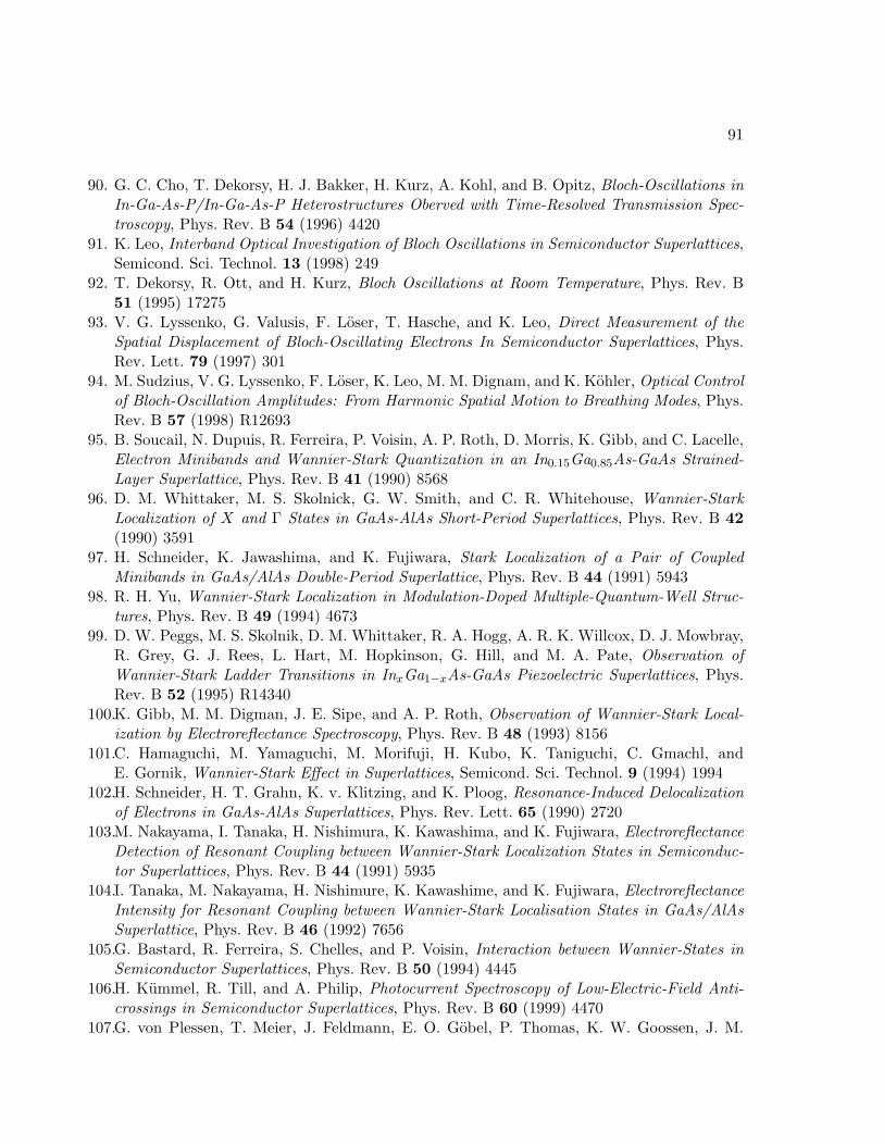
91

90. G. C. Cho, T. Dekorsy, H. J. Bakker, H. Kurz, A. Kohl, and B. Opitz, Bloch-Oscillations inIn-Ga-As-P/In-Ga-As-P Heterostructures Oberved with Time-Resolved Transmission Spec-troscopy, Phys. Rev. B 54 (1996) 4420

91. K. Leo, Interband Optical Investigation of Bloch Oscillations in Semiconductor Superlattices,Semicond. Sci. Technol. 13 (1998) 249

92. T. Dekorsy, R. Ott, and H. Kurz, Bloch Oscillations at Room Temperature, Phys. Rev. B51 (1995) 17275

93. V. G. Lyssenko, G. Valusis, F. Loser, T. Hasche, and K. Leo, Direct Measurement of theSpatial Displacement of Bloch-Oscillating Electrons In Semiconductor Superlattices, Phys.Rev. Lett. 79 (1997) 301

94. M. Sudzius, V. G. Lyssenko, F. Loser, K. Leo, M. M. Dignam, and K. Kohler, Optical Controlof Bloch-Oscillation Amplitudes: From Harmonic Spatial Motion to Breathing Modes, Phys.Rev. B 57 (1998) R12693

95. B. Soucail, N. Dupuis, R. Ferreira, P. Voisin, A. P. Roth, D. Morris, K. Gibb, and C. Lacelle,Electron Minibands and Wannier-Stark Quantization in an In0.15Ga0.85As-GaAs Strained-Layer Superlattice, Phys. Rev. B 41 (1990) 8568

96. D. M. Whittaker, M. S. Skolnick, G. W. Smith, and C. R. Whitehouse, Wannier-StarkLocalization of X and Γ States in GaAs-AlAs Short-Period Superlattices, Phys. Rev. B 42(1990) 3591

97. H. Schneider, K. Jawashima, and K. Fujiwara, Stark Localization of a Pair of CoupledMinibands in GaAs/AlAs Double-Period Superlattice, Phys. Rev. B 44 (1991) 5943

98. R. H. Yu, Wannier-Stark Localization in Modulation-Doped Multiple-Quantum-Well Struc-tures, Phys. Rev. B 49 (1994) 4673

99. D. W. Peggs, M. S. Skolnik, D. M. Whittaker, R. A. Hogg, A. R. K. Willcox, D. J. Mowbray,R. Grey, G. J. Rees, L. Hart, M. Hopkinson, G. Hill, and M. A. Pate, Observation ofWannier-Stark Ladder Transitions in InxGa1−xAs-GaAs Piezoelectric Superlattices, Phys.Rev. B 52 (1995) R14340

100.K. Gibb, M. M. Digman, J. E. Sipe, and A. P. Roth, Observation of Wannier-Stark Local-ization by Electroreflectance Spectroscopy, Phys. Rev. B 48 (1993) 8156

101.C. Hamaguchi, M. Yamaguchi, M. Morifuji, H. Kubo, K. Taniguchi, C. Gmachl, andE. Gornik, Wannier-Stark Effect in Superlattices, Semicond. Sci. Technol. 9 (1994) 1994

102.H. Schneider, H. T. Grahn, K. v. Klitzing, and K. Ploog, Resonance-Induced Delocalizationof Electrons in GaAs-AlAs Superlattices, Phys. Rev. Lett. 65 (1990) 2720

103.M. Nakayama, I. Tanaka, H. Nishimura, K. Kawashima, and K. Fujiwara, ElectroreflectanceDetection of Resonant Coupling between Wannier-Stark Localization States in Semiconduc-tor Superlattices, Phys. Rev. B 44 (1991) 5935

104.I. Tanaka, M. Nakayama, H. Nishimure, K. Kawashime, and K. Fujiwara, ElectroreflectanceIntensity for Resonant Coupling between Wannier-Stark Localisation States in GaAs/AlAsSuperlattice, Phys. Rev. B 46 (1992) 7656

105.G. Bastard, R. Ferreira, S. Chelles, and P. Voisin, Interaction between Wannier-States inSemiconductor Superlattices, Phys. Rev. B 50 (1994) 4445

106.H. Kummel, R. Till, and A. Philip, Photocurrent Spectroscopy of Low-Electric-Field Anti-crossings in Semiconductor Superlattices, Phys. Rev. B 60 (1999) 4470

107.G. von Plessen, T. Meier, J. Feldmann, E. O. Gobel, P. Thomas, K. W. Goossen, J. M.

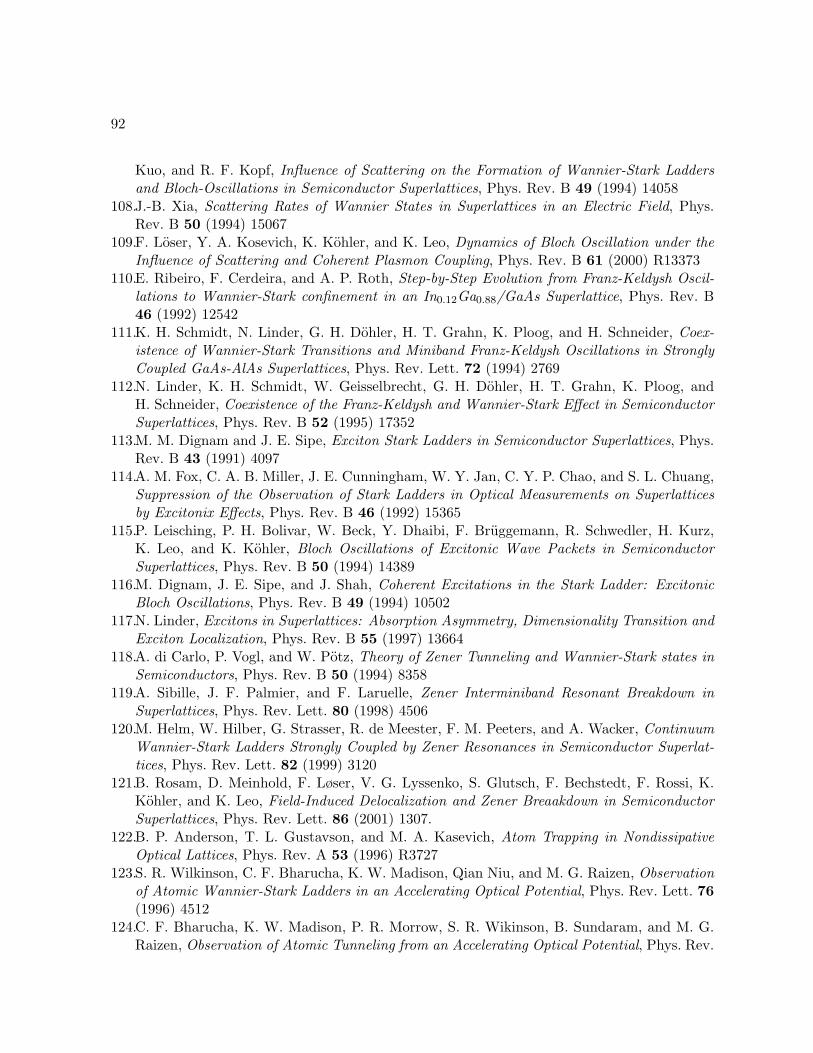
92

Kuo, and R. F. Kopf, Influence of Scattering on the Formation of Wannier-Stark Laddersand Bloch-Oscillations in Semiconductor Superlattices, Phys. Rev. B 49 (1994) 14058

108.J.-B. Xia, Scattering Rates of Wannier States in Superlattices in an Electric Field, Phys.Rev. B 50 (1994) 15067

109.F. Loser, Y. A. Kosevich, K. Kohler, and K. Leo, Dynamics of Bloch Oscillation under theInfluence of Scattering and Coherent Plasmon Coupling, Phys. Rev. B 61 (2000) R13373

110.E. Ribeiro, F. Cerdeira, and A. P. Roth, Step-by-Step Evolution from Franz-Keldysh Oscil-lations to Wannier-Stark confinement in an In0.12Ga0.88/GaAs Superlattice, Phys. Rev. B46 (1992) 12542

111.K. H. Schmidt, N. Linder, G. H. Dohler, H. T. Grahn, K. Ploog, and H. Schneider, Coex-istence of Wannier-Stark Transitions and Miniband Franz-Keldysh Oscillations in StronglyCoupled GaAs-AlAs Superlattices, Phys. Rev. Lett. 72 (1994) 2769

112.N. Linder, K. H. Schmidt, W. Geisselbrecht, G. H. Dohler, H. T. Grahn, K. Ploog, andH. Schneider, Coexistence of the Franz-Keldysh and Wannier-Stark Effect in SemiconductorSuperlattices, Phys. Rev. B 52 (1995) 17352

113.M. M. Dignam and J. E. Sipe, Exciton Stark Ladders in Semiconductor Superlattices, Phys.Rev. B 43 (1991) 4097

114.A. M. Fox, C. A. B. Miller, J. E. Cunningham, W. Y. Jan, C. Y. P. Chao, and S. L. Chuang,Suppression of the Observation of Stark Ladders in Optical Measurements on Superlatticesby Excitonix Effects, Phys. Rev. B 46 (1992) 15365

115.P. Leisching, P. H. Bolivar, W. Beck, Y. Dhaibi, F. Bruggemann, R. Schwedler, H. Kurz,K. Leo, and K. Kohler, Bloch Oscillations of Excitonic Wave Packets in SemiconductorSuperlattices, Phys. Rev. B 50 (1994) 14389

116.M. Dignam, J. E. Sipe, and J. Shah, Coherent Excitations in the Stark Ladder: ExcitonicBloch Oscillations, Phys. Rev. B 49 (1994) 10502

117.N. Linder, Excitons in Superlattices: Absorption Asymmetry, Dimensionality Transition andExciton Localization, Phys. Rev. B 55 (1997) 13664

118.A. di Carlo, P. Vogl, and W. Potz, Theory of Zener Tunneling and Wannier-Stark states inSemiconductors, Phys. Rev. B 50 (1994) 8358

119.A. Sibille, J. F. Palmier, and F. Laruelle, Zener Interminiband Resonant Breakdown inSuperlattices, Phys. Rev. Lett. 80 (1998) 4506

120.M. Helm, W. Hilber, G. Strasser, R. de Meester, F. M. Peeters, and A. Wacker, ContinuumWannier-Stark Ladders Strongly Coupled by Zener Resonances in Semiconductor Superlat-tices, Phys. Rev. Lett. 82 (1999) 3120

121.B. Rosam, D. Meinhold, F. Løser, V. G. Lyssenko, S. Glutsch, F. Bechstedt, F. Rossi, K.Kohler, and K. Leo, Field-Induced Delocalization and Zener Breaakdown in SemiconductorSuperlattices, Phys. Rev. Lett. 86 (2001) 1307.

122.B. P. Anderson, T. L. Gustavson, and M. A. Kasevich, Atom Trapping in NondissipativeOptical Lattices, Phys. Rev. A 53 (1996) R3727

123.S. R. Wilkinson, C. F. Bharucha, K. W. Madison, Qian Niu, and M. G. Raizen, Observationof Atomic Wannier-Stark Ladders in an Accelerating Optical Potential, Phys. Rev. Lett. 76(1996) 4512

124.C. F. Bharucha, K. W. Madison, P. R. Morrow, S. R. Wikinson, B. Sundaram, and M. G.Raizen, Observation of Atomic Tunneling from an Accelerating Optical Potential, Phys. Rev.

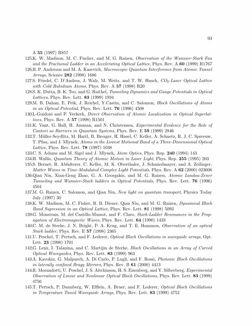
93

A 55 (1997) R857125.K. W. Madison, M. C. Fischer, and M. G. Raizen, Observation of the Wannier-Stark Fan

and the Fractional Ladder in an Accelerating Optical Lattice, Phys. Rev. A 60 (1999) R1767126.B. P. Anderson and M. A. Kasevich, Macroscopic Quantum Interference from Atomic Tunnel

Arrays, Science 282 (1998) 1686127.S. Friedel, C. D’Andrea, J. Walz, M. Weitz, and T. W. Hnsch, CO2-Laser Optical Lattice

with Cold Rubidium Atoms, Phys. Rev. A 57 (1998) R20128.S. K. Dutta, B. K. Teo, and G. Raithel, Tunneling Dynamics and Gauge Potentials in Optical

Lattices, Phys. Rev. Lett. 83 (1999) 1934129.M. B. Dahan, E. Peik, J. Reichel, Y.Castin, and C. Salomon, Bloch Oscillations of Atoms

in an Optical Potential, Phys. Rev. Lett. 76 (1996) 4508130.L-Guidoni and P. Verkerk, Direct Observation of Atomic Localization in Optical Superlat-

tices, Phys. Rev. A 57 (1998) R1501131.K. Vant, G. Ball, H. Amman, and N. Christensen, Experimental Evidence for the Role of

Cantori as Barriers in Quantum Systems, Phys. Rev. E 59 (1999) 2846132.T. Muller-Seydlitz, M. Hartl, B. Brezger, H. Hnsel, C. Keller, A. Schnetz, R. J. C. Spreeuw,

T. Pfau, and J. Mlynek, Atoms in the Lowest Motional Band of a Three-Dimensional OpticalLattice, Phys. Rev. Lett. 78 (1997) 1038

133.C. S. Adams and M. Sigel and J. Mlynek, Atom Optics, Phys. Rep. 240 (1994) 143134.H. Wallis, Quantum Theory of Atomic Motion in Laser Light, Phys. Rep. 255 (1995) 203135.S. Bernet, R. Abfalterer, C. Keller, M. K. Oberthaler, J. Schmiedmayer, and A. Zeilinger,

Matter Waves in Time-Modulated Complex Light Potentials, Phys. Rev. A 62 (2000) 023606136.Qian Niu, Xian-Geng Zhao, G. A. Georgakis, and M. G. Raizen, Atomic Landau-Zener

Tunneling and Wannier-Stark ladders in Optical Potentials, Phys. Rev. Lett. 76 (1996)4504

137.M. G. Raizen, C. Salomon, and Qian Niu, New light on quantum transport, Physics TodayJuly (1997) 30

138.K. W. Madison, M. C. Fisher, R. B. Diener, Qian Niu, and M. G. Raizen, Dynamical BlochBand Supression in an Optical Lattice, Phys. Rev. Lett. 81 (1998) 5093

139.G. Monsivais, M. del Castillo-Mussot, and F. Claro, Stark-Ladder Resonances in the Prop-agation of Electromagnetic Waves, Phys. Rev. Lett. 64 (1990) 1433

140.C. M. de Sterke, J. N. Bright, P. A. Krug, and T. E. Hammon, Observation of an opticalStark ladder, Phys. Rev. E 57 (1998) 2365

141.U. Peschel, T. Pertsch, and F. Lederer, Optical Bloch Oscillations in waveguide arrays, Opt.Lett. 23 (1998) 1701

142.G. Lenz, I. Talanina, and C. Martijin de Sterke, Bloch Oscillations in an Array of CurvedOptical Waveguides, Phys. Rev. Lett. 83 (1999) 963

143.A. Kavokin, G. Malpuech, A. Di Carlo, P. Lugli, and F. Rossi, Photonic Bloch Oscillationsin laterally confined Bragg Mirrors, Phys. Rev. B 61 (2000) 4413

144.R. Morandotti, U. Peschel, J. S. Aitchinson, H. S. Eisenberg, and Y. Silberberg, ExperimentalObservation of Linear and Nonlinear Optical Bloch Oscillations, Phys. Rev. Lett. 83 (1999)4756

145.T. Pertsch, P. Dannberg, W. Elflein, A. Bruer, and F. Lederer, Optical Bloch Oscillationsin Temperature Tuned Waveguide Arrays, Phys. Rev. Lett. 83 (1999) 4752

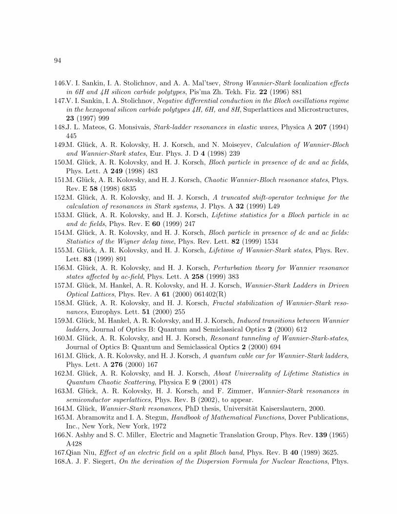
94

146.V. I. Sankin, I. A. Stolichnov, and A. A. Mal’tsev, Strong Wannier-Stark localization effectsin 6H and 4H silicon carbide polytypes, Pis’ma Zh. Tekh. Fiz. 22 (1996) 881

147.V. I. Sankin, I. A. Stolichnov, Negative differential conduction in the Bloch oscillations regimein the hexagonal silicon carbide polytypes 4H, 6H, and 8H, Superlattices and Microstructures,23 (1997) 999

148.J. L. Mateos, G. Monsivais, Stark-ladder resonances in elastic waves, Physica A 207 (1994)445

149.M. Gluck, A. R. Kolovsky, H. J. Korsch, and N. Moiseyev, Calculation of Wannier-Blochand Wannier-Stark states, Eur. Phys. J. D 4 (1998) 239

150.M. Gluck, A. R. Kolovsky, and H. J. Korsch, Bloch particle in presence of dc and ac fields,Phys. Lett. A 249 (1998) 483

151.M. Gluck, A. R. Kolovsky, and H. J. Korsch, Chaotic Wannier-Bloch resonance states, Phys.Rev. E 58 (1998) 6835

152.M. Gluck, A. R. Kolovsky, and H. J. Korsch, A truncated shift-operator technique for thecalculation of resonances in Stark systems, J. Phys. A 32 (1999) L49

153.M. Gluck, A. R. Kolovsky, and H. J. Korsch, Lifetime statistics for a Bloch particle in acand dc fields, Phys. Rev. E 60 (1999) 247

154.M. Gluck, A. R. Kolovsky, and H. J. Korsch, Bloch particle in presence of dc and ac fields:Statistics of the Wigner delay time, Phys. Rev. Lett. 82 (1999) 1534

155.M. Gluck, A. R. Kolovsky, and H. J. Korsch, Lifetime of Wannier-Stark states, Phys. Rev.Lett. 83 (1999) 891

156.M. Gluck, A. R. Kolovsky, and H. J. Korsch, Perturbation theory for Wannier resonancestates affected by ac-field, Phys. Lett. A 258 (1999) 383

157.M. Gluck, M. Hankel, A. R. Kolovsky, and H. J. Korsch, Wannier-Stark Ladders in DrivenOptical Lattices, Phys. Rev. A 61 (2000) 061402(R)

158.M. Gluck, A. R. Kolovsky, and H. J. Korsch, Fractal stabilization of Wannier-Stark reso-nances, Europhys. Lett. 51 (2000) 255

159.M. Gluck, M. Hankel, A. R. Kolovsky, and H. J. Korsch, Induced transitions between Wannierladders, Journal of Optics B: Quantum and Semiclassical Optics 2 (2000) 612

160.M. Gluck, A. R. Kolovsky, and H. J. Korsch, Resonant tunneling of Wannier-Stark-states,Journal of Optics B: Quantum and Semiclassical Optics 2 (2000) 694

161.M. Gluck, A. R. Kolovsky, and H. J. Korsch, A quantum cable car for Wannier-Stark ladders,Phys. Lett. A 276 (2000) 167

162.M. Gluck, A. R. Kolovsky, and H. J. Korsch, About Universality of Lifetime Statistics inQuantum Chaotic Scattering, Physica E 9 (2001) 478

163.M. Gluck, A. R. Kolovsky, H. J. Korsch, and F. Zimmer, Wannier-Stark resonances insemiconductor superlattices, Phys. Rev. B (2002), to appear.

164.M. Gluck, Wannier-Stark resonances, PhD thesis, Universitat Kaiserslautern, 2000.165.M. Abramowitz and I. A. Stegun, Handbook of Mathematical Functions, Dover Publications,

Inc., New York, New York, 1972166.N. Ashby and S. C. Miller, Electric and Magnetic Translation Group, Phys. Rev. 139 (1965)

A428167.Qian Niu, Effect of an electric field on a split Bloch band, Phys. Rev. B 40 (1989) 3625.168.A. J. F. Siegert, On the derivation of the Dispersion Formula for Nuclear Reactions, Phys.

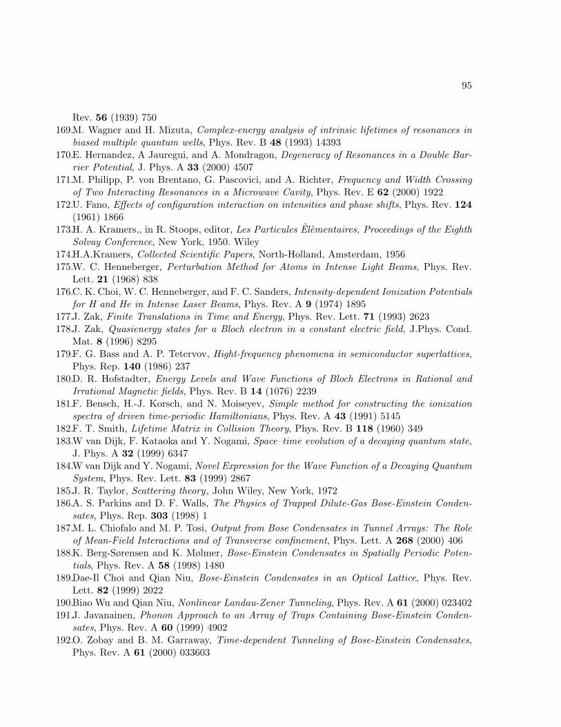
95

Rev. 56 (1939) 750169.M. Wagner and H. Mizuta, Complex-energy analysis of intrinsic lifetimes of resonances in

biased multiple quantum wells, Phys. Rev. B 48 (1993) 14393170.E. Hernandez, A Jauregui, and A. Mondragon, Degeneracy of Resonances in a Double Bar-

rier Potential, J. Phys. A 33 (2000) 4507171.M. Philipp, P. von Brentano, G. Pascovici, and A. Richter, Frequency and Width Crossing

of Two Interacting Resonances in a Microwave Cavity, Phys. Rev. E 62 (2000) 1922172.U. Fano, Effects of configuration interaction on intensities and phase shifts, Phys. Rev. 124

(1961) 1866173.H. A. Kramers,, in R. Stoops, editor, Les Particules Elementaires, Proceedings of the Eighth

Solvay Conference, New York, 1950. Wiley174.H.A.Kramers, Collected Scientific Papers, North-Holland, Amsterdam, 1956175.W. C. Henneberger, Perturbation Method for Atoms in Intense Light Beams, Phys. Rev.

Lett. 21 (1968) 838176.C. K. Choi, W. C. Henneberger, and F. C. Sanders, Intensity-dependent Ionization Potentials

for H and He in Intense Laser Beams, Phys. Rev. A 9 (1974) 1895177.J. Zak, Finite Translations in Time and Energy, Phys. Rev. Lett. 71 (1993) 2623178.J. Zak, Quasienergy states for a Bloch electron in a constant electric field, J.Phys. Cond.

Mat. 8 (1996) 8295179.F. G. Bass and A. P. Tetervov, Hight-frequency phenomena in semiconductor superlattices,

Phys. Rep. 140 (1986) 237180.D. R. Hofstadter, Energy Levels and Wave Functions of Bloch Electrons in Rational and

Irrational Magnetic fields, Phys. Rev. B 14 (1076) 2239181.F. Bensch, H.-J. Korsch, and N. Moiseyev, Simple method for constructing the ionization

spectra of driven time-periodic Hamiltonians, Phys. Rev. A 43 (1991) 5145182.F. T. Smith, Lifetime Matrix in Collision Theory, Phys. Rev. B 118 (1960) 349183.W van Dijk, F. Kataoka and Y. Nogami, Space–time evolution of a decaying quantum state,

J. Phys. A 32 (1999) 6347184.W van Dijk and Y. Nogami, Novel Expression for the Wave Function of a Decaying Quantum

System, Phys. Rev. Lett. 83 (1999) 2867185.J. R. Taylor, Scattering theory , John Wiley, New York, 1972186.A. S. Parkins and D. F. Walls, The Physics of Trapped Dilute-Gas Bose-Einstein Conden-

sates, Phys. Rep. 303 (1998) 1187.M. L. Chiofalo and M. P. Tosi, Output from Bose Condensates in Tunnel Arrays: The Role

of Mean-Field Interactions and of Transverse confinement, Phys. Lett. A 268 (2000) 406188.K. Berg-Sørensen and K. Mølmer, Bose-Einstein Condensates in Spatially Periodic Poten-

tials, Phys. Rev. A 58 (1998) 1480189.Dae-Il Choi and Qian Niu, Bose-Einstein Condensates in an Optical Lattice, Phys. Rev.

Lett. 82 (1999) 2022190.Biao Wu and Qian Niu, Nonlinear Landau-Zener Tunneling, Phys. Rev. A 61 (2000) 023402191.J. Javanainen, Phonon Approach to an Array of Traps Containing Bose-Einstein Conden-

sates, Phys. Rev. A 60 (1999) 4902192.O. Zobay and B. M. Garraway, Time-dependent Tunneling of Bose-Einstein Condensates,

Phys. Rev. A 61 (2000) 033603

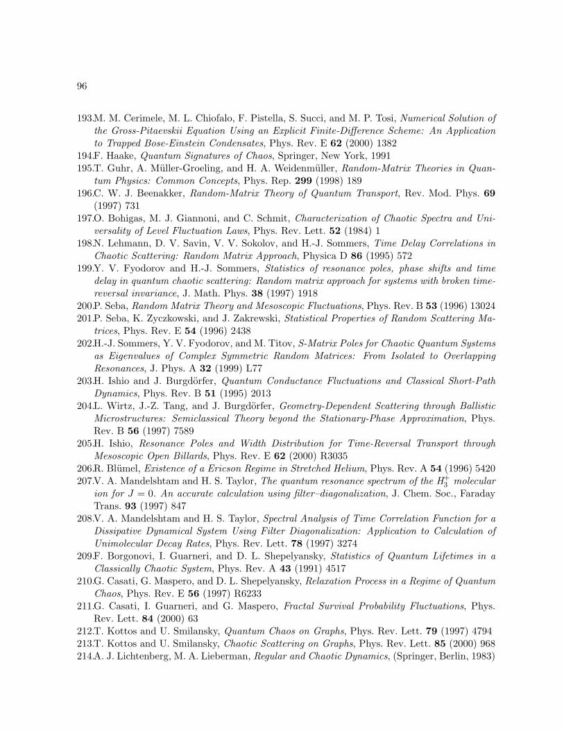
96

193.M. M. Cerimele, M. L. Chiofalo, F. Pistella, S. Succi, and M. P. Tosi, Numerical Solution ofthe Gross-Pitaevskii Equation Using an Explicit Finite-Difference Scheme: An Applicationto Trapped Bose-Einstein Condensates, Phys. Rev. E 62 (2000) 1382

194.F. Haake, Quantum Signatures of Chaos, Springer, New York, 1991195.T. Guhr, A. Muller-Groeling, and H. A. Weidenmuller, Random-Matrix Theories in Quan-

tum Physics: Common Concepts, Phys. Rep. 299 (1998) 189196.C. W. J. Beenakker, Random-Matrix Theory of Quantum Transport, Rev. Mod. Phys. 69

(1997) 731197.O. Bohigas, M. J. Giannoni, and C. Schmit, Characterization of Chaotic Spectra and Uni-

versality of Level Fluctuation Laws, Phys. Rev. Lett. 52 (1984) 1198.N. Lehmann, D. V. Savin, V. V. Sokolov, and H.-J. Sommers, Time Delay Correlations in

Chaotic Scattering: Random Matrix Approach, Physica D 86 (1995) 572199.Y. V. Fyodorov and H.-J. Sommers, Statistics of resonance poles, phase shifts and time

delay in quantum chaotic scattering: Random matrix approach for systems with broken time-reversal invariance, J. Math. Phys. 38 (1997) 1918

200.P. Seba, Random Matrix Theory and Mesoscopic Fluctuations, Phys. Rev. B 53 (1996) 13024201.P. Seba, K. Zyczkowski, and J. Zakrewski, Statistical Properties of Random Scattering Ma-

trices, Phys. Rev. E 54 (1996) 2438202.H.-J. Sommers, Y. V. Fyodorov, and M. Titov, S-Matrix Poles for Chaotic Quantum Systems

as Eigenvalues of Complex Symmetric Random Matrices: From Isolated to OverlappingResonances, J. Phys. A 32 (1999) L77

203.H. Ishio and J. Burgdorfer, Quantum Conductance Fluctuations and Classical Short-PathDynamics, Phys. Rev. B 51 (1995) 2013

204.L. Wirtz, J.-Z. Tang, and J. Burgdorfer, Geometry-Dependent Scattering through BallisticMicrostructures: Semiclassical Theory beyond the Stationary-Phase Approximation, Phys.Rev. B 56 (1997) 7589

205.H. Ishio, Resonance Poles and Width Distribution for Time-Reversal Transport throughMesoscopic Open Billards, Phys. Rev. E 62 (2000) R3035

206.R. Blumel, Existence of a Ericson Regime in Stretched Helium, Phys. Rev. A 54 (1996) 5420207.V. A. Mandelshtam and H. S. Taylor, The quantum resonance spectrum of the H+

3 molecularion for J = 0. An accurate calculation using filter–diagonalization, J. Chem. Soc., FaradayTrans. 93 (1997) 847

208.V. A. Mandelshtam and H. S. Taylor, Spectral Analysis of Time Correlation Function for aDissipative Dynamical System Using Filter Diagonalization: Application to Calculation ofUnimolecular Decay Rates, Phys. Rev. Lett. 78 (1997) 3274

209.F. Borgonovi, I. Guarneri, and D. L. Shepelyansky, Statistics of Quantum Lifetimes in aClassically Chaotic System, Phys. Rev. A 43 (1991) 4517

210.G. Casati, G. Maspero, and D. L. Shepelyansky, Relaxation Process in a Regime of QuantumChaos, Phys. Rev. E 56 (1997) R6233

211.G. Casati, I. Guarneri, and G. Maspero, Fractal Survival Probability Fluctuations, Phys.Rev. Lett. 84 (2000) 63

212.T. Kottos and U. Smilansky, Quantum Chaos on Graphs, Phys. Rev. Lett. 79 (1997) 4794213.T. Kottos and U. Smilansky, Chaotic Scattering on Graphs, Phys. Rev. Lett. 85 (2000) 968214.A. J. Lichtenberg, M. A. Lieberman, Regular and Chaotic Dynamics, (Springer, Berlin, 1983)

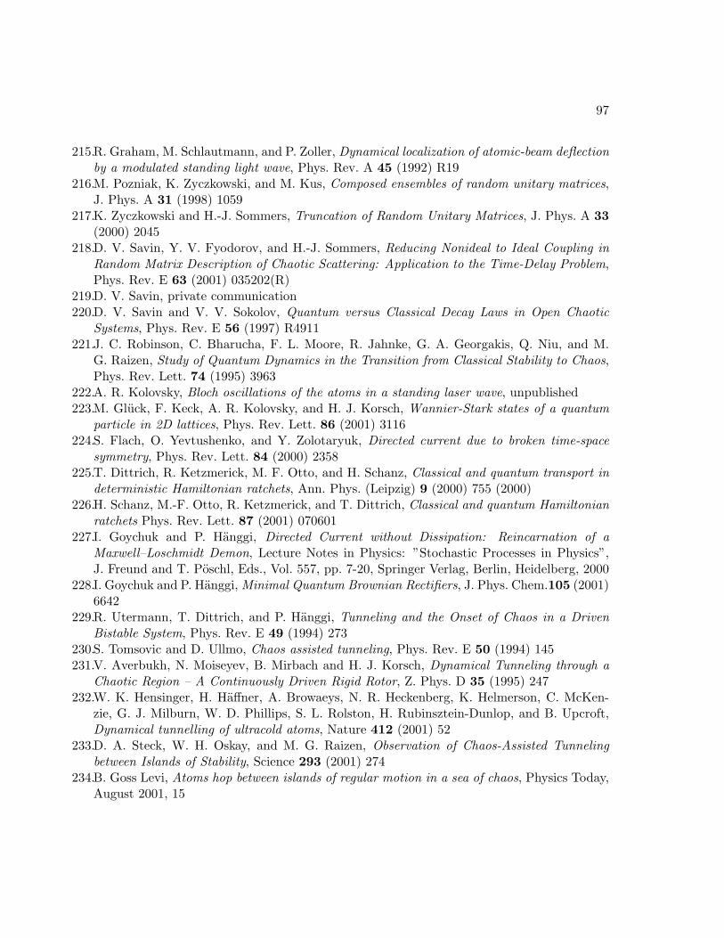
97

215.R. Graham, M. Schlautmann, and P. Zoller, Dynamical localization of atomic-beam deflectionby a modulated standing light wave, Phys. Rev. A 45 (1992) R19

216.M. Pozniak, K. Zyczkowski, and M. Kus, Composed ensembles of random unitary matrices,J. Phys. A 31 (1998) 1059

217.K. Zyczkowski and H.-J. Sommers, Truncation of Random Unitary Matrices, J. Phys. A 33(2000) 2045

218.D. V. Savin, Y. V. Fyodorov, and H.-J. Sommers, Reducing Nonideal to Ideal Coupling inRandom Matrix Description of Chaotic Scattering: Application to the Time-Delay Problem,Phys. Rev. E 63 (2001) 035202(R)

219.D. V. Savin, private communication220.D. V. Savin and V. V. Sokolov, Quantum versus Classical Decay Laws in Open Chaotic

Systems, Phys. Rev. E 56 (1997) R4911221.J. C. Robinson, C. Bharucha, F. L. Moore, R. Jahnke, G. A. Georgakis, Q. Niu, and M.

G. Raizen, Study of Quantum Dynamics in the Transition from Classical Stability to Chaos,Phys. Rev. Lett. 74 (1995) 3963

222.A. R. Kolovsky, Bloch oscillations of the atoms in a standing laser wave, unpublished223.M. Gluck, F. Keck, A. R. Kolovsky, and H. J. Korsch, Wannier-Stark states of a quantum

particle in 2D lattices, Phys. Rev. Lett. 86 (2001) 3116224.S. Flach, O. Yevtushenko, and Y. Zolotaryuk, Directed current due to broken time-space

symmetry, Phys. Rev. Lett. 84 (2000) 2358225.T. Dittrich, R. Ketzmerick, M. F. Otto, and H. Schanz, Classical and quantum transport in

deterministic Hamiltonian ratchets, Ann. Phys. (Leipzig) 9 (2000) 755 (2000)226.H. Schanz, M.-F. Otto, R. Ketzmerick, and T. Dittrich, Classical and quantum Hamiltonian

ratchets Phys. Rev. Lett. 87 (2001) 070601227.I. Goychuk and P. Hanggi, Directed Current without Dissipation: Reincarnation of a

Maxwell–Loschmidt Demon, Lecture Notes in Physics: ”Stochastic Processes in Physics”,J. Freund and T. Poschl, Eds., Vol. 557, pp. 7-20, Springer Verlag, Berlin, Heidelberg, 2000

228.I. Goychuk and P. Hanggi, Minimal Quantum Brownian Rectifiers, J. Phys. Chem.105 (2001)6642

229.R. Utermann, T. Dittrich, and P. Hanggi, Tunneling and the Onset of Chaos in a DrivenBistable System, Phys. Rev. E 49 (1994) 273

230.S. Tomsovic and D. Ullmo, Chaos assisted tunneling, Phys. Rev. E 50 (1994) 145231.V. Averbukh, N. Moiseyev, B. Mirbach and H. J. Korsch, Dynamical Tunneling through a

Chaotic Region – A Continuously Driven Rigid Rotor, Z. Phys. D 35 (1995) 247232.W. K. Hensinger, H. Haffner, A. Browaeys, N. R. Heckenberg, K. Helmerson, C. McKen-

zie, G. J. Milburn, W. D. Phillips, S. L. Rolston, H. Rubinsztein-Dunlop, and B. Upcroft,Dynamical tunnelling of ultracold atoms, Nature 412 (2001) 52

233.D. A. Steck, W. H. Oskay, and M. G. Raizen, Observation of Chaos-Assisted Tunnelingbetween Islands of Stability, Science 293 (2001) 274

234.B. Goss Levi, Atoms hop between islands of regular motion in a sea of chaos, Physics Today,August 2001, 15