Embed Size (px)
Citation preview
Robert Johannes Triebl, BSc
Wannier charge centers and the
calculation of topological
invariants: Application to the
Kane-Mele-Hubbard model
MASTER THESIS
For obtaining the academic degree
Diplom-Ingenieur
Master Programme of
Technical Physics
Graz University of Technology
Supervisor:
Univ.-Prof. Dr.rer.nat. Enrico Arrigoni
Co-Supervisor:
Dr.techn. Markus Aichhorn
Institute of Theoretical and Computational Physics
Graz, March 2015

Acknowledgements
I would like to thank Prof. Arrigoni for the supervision of my work. He wasa great help in understanding concepts of many-body physics and had alwaystime for questions and concerns.
Furthermore, I owe my gratitude to Markus Aichhorn. He was the drivingforce in developing the framework of this thesis and helped a lot with distin-guished advice, always willing to listen to me.
I am thankful to Prof. von der Linden for helpful discussion. I am alsograteful to the other members of the Institute of Theoretical and Computa-tional Physics for the great atmosphere and their willingness to discuss upcom-ing problems. Here I would like to emphasize Manuel Zingl, whose cooperationhelped me to solve many minor problems of daily work.
Last but not least I would like to thank my parents and my whole family,who have always been there for me and helped me in all regards.
3

4
Abstract
Topological insulators are a class of materials different from trivial band insu-lators. The topological order of the insulators, classified by invariants, is thereason for gapless states emerging at the surface. Currently, they are in thespotlight of theoretical as well as experimental physics due to the possible ap-plications of such edge states in quantum computing. Of certain interest is theinfluence of strong electron-electron interaction, which is investigated in thisthesis. The system used here is the Kane-Mele-Hubbard (KMH) model, whichis an interacting two-dimensional tight-binding model on a honeycomb lattice.Unlike trivial models for graphene, a spin-orbit coupling is added that gapsthe system and leads to a nontrivial topology. To test a possible evaluation oftopological invariants using Wannier charge centers (WCC), the noninteractingKane-Mele model is analyzed in detail. The Hubbard term is first introduced inmean-field (MF) approximation in order to keep the determination of invariantsusing WCC possible, which requires the existence of Bloch functions. Usingthis tool, the phase diagram of the KMH model is determined as a functionof interaction strength, spin-orbit coupling, on-site potential and Rashba cou-pling. The resulting topological invariants are compared to the existence of edgestates of the MF-KMH model on a zigzag ribbon, showing perfect agreement.Finally, a two-site dynamical impurity approximation (DIA) which is based onthe self-energy-functional approach is used to obtain results beyond MF. Thetopological invariants of this fully interacting system are determined using a so-called topological Hamiltonian in order to allow a calculation with WCC. TheDIA results show that the direction of a possible magnetic moment is of greatimportance in order to calculate topological properties.
5

6
Kurzfassung
Topologische Isolatoren sind eine Klasse von Materialien, die sich von gewohn-lichen Band-Isolatoren unterscheiden. Die topologische Ordnung der Isolatoren,klassifiziert durch Invarianten, ist der Grund fur die Existenz von Zustandenohne Bandlucke an der Oberflache. Derzeit sind sie wegen moglicher Anwendun-gen dieser Randzustande in der Quanteninformatik im Rampenlicht sowohl inder theoretische, als auch der experimentellen Physik. Von besonderem Interesseist der Einfluss von starker Wechselwirkung der Elektronen, die in dieser Arbeituntersucht wird. Das System, das hier verwendet wird, ist das Kane-Mele-Hubbard-Modell (KMH), welches ein zweidimensionales Tight-Binding-Modellauf einem Bienenwabengitter ist. Im Unterschied zu einfachen Modellen vonGraphen ist eine Spin-Orbit-Kopplung hinzugefugt, die eine Bandlucke und dienichttriviale Topologie verursacht. Um eine mogliche Bestimmung von topolo-gischen Invarianten unter Verwendung von Wannier-Zentren zu testen, wird dasnichtwechselwirkende Kane-Mele-Modell im Detail analysiert. Der Hubbard-Term wird zuerst in einer Mean-Field-Naherung (MF) eingefuhrt, um die Bes-timmung von Invarianten mit Wannier-Zentren zu ermoglichen, welche die Exis-tenz von Bloch-Zustanden voraussetzen. Mit dieser Methode wird das Phasendi-agramm des KMH-Modells in Abhangigkeit von der Wechselwirkungsstarke, derSpin-Orbit-Kopplung, einer Energiedifferenz zwischen den Untergittern, undder Rashba-Kopplung bestimmt. Die topologischen Invarianten werden mitder Existenz von Randzustanden des MF-KMH-Modells verglichen und zeigenperfekte Ubereinstimmung. Zum Abschluss wurde eine dynamische Storstellen-Naherung (DIA) auf zwei Platzen, die auf der Selbstenergie-Funktional-Methodefußt, verwendet, um Resultate zu erzielen, die uber MF hinausgehen. Dietopologischen Invarianten dieses wechselwirkenden Systems wurden mit einemso genannten topologischen Hamilton-Operator bestimmt, um die Berechnungmit Wannier-Zentren zu erlauben. Die DIA Resultate zeigen, dass die Rich-tung eines moglichen magnetischen Momentes von großer Wichtigkeit sind, umtopologische Eigenschaften zu berechnen.
7

8
Contents
1 Topological invariants 11
1.1 Berry phase . . . . . . . . . . . . . . . . . . . . . . . . . . . . . . 11
1.2 Chern invariant . . . . . . . . . . . . . . . . . . . . . . . . . . . . 12
1.3 Integer Quantum Hall effect . . . . . . . . . . . . . . . . . . . . . 13
1.3.1 Quantum Spin Hall insulator . . . . . . . . . . . . . . . . 15
1.4 Time reversal symmetry . . . . . . . . . . . . . . . . . . . . . . . 16
1.5 Theory of charge polarisation - Wannier functions . . . . . . . . 17
1.6 Definition of Z2 invariant by Fu and Kane . . . . . . . . . . . . . 18
1.6.1 Topological systems with inversion symmetry . . . . . . . 21
1.7 Soluyanov-Vanderbilt method . . . . . . . . . . . . . . . . . . . . 21
1.8 Topological invariants for interacting systems . . . . . . . . . . . 25
1.9 Bulk boundary correspondence . . . . . . . . . . . . . . . . . . . 27
2 The Kane-Mele model 31
2.1 Graphene . . . . . . . . . . . . . . . . . . . . . . . . . . . . . . . 31
2.2 Haldane model . . . . . . . . . . . . . . . . . . . . . . . . . . . . 34
2.3 Kane-Mele model . . . . . . . . . . . . . . . . . . . . . . . . . . . 35
2.3.1 Bloch Hamiltonian . . . . . . . . . . . . . . . . . . . . . . 36
2.3.2 Topology in inversion symmetric case . . . . . . . . . . . 38
2.3.3 Topology in general case . . . . . . . . . . . . . . . . . . . 40
2.4 Ribbon . . . . . . . . . . . . . . . . . . . . . . . . . . . . . . . . 44
2.4.1 Geometry . . . . . . . . . . . . . . . . . . . . . . . . . . . 44
2.4.2 Kane-Mele model on a zigzag ribbon . . . . . . . . . . . . 48
3 Kane-Mele-Hubbard model 53
3.1 Magnetisation . . . . . . . . . . . . . . . . . . . . . . . . . . . . . 54
3.2 Topological transitions . . . . . . . . . . . . . . . . . . . . . . . . 56
3.2.1 Generalisation of Z2 invariant definition . . . . . . . . . . 58
3.3 Influence of a sublattice potential . . . . . . . . . . . . . . . . . . 59
3.4 Influence of Rashba coupling . . . . . . . . . . . . . . . . . . . . 63
3.5 KMH model on a zigzag ribbon . . . . . . . . . . . . . . . . . . . 68
3.5.1 Magnetisation . . . . . . . . . . . . . . . . . . . . . . . . . 68
3.5.2 Topology and edge states . . . . . . . . . . . . . . . . . . 69
4 KMH beyond mean-field 73
4.1 Self-energy-functional approach . . . . . . . . . . . . . . . . . . . 73
4.2 Kane-Mele-Hubbard model in 2 site DIA . . . . . . . . . . . . . . 76
9
10 CONTENTS
5 Conclusions and outlook 83
A Kane-Mele Bloch Hamiltonians 85A.1 Bulk . . . . . . . . . . . . . . . . . . . . . . . . . . . . . . . . . . 85A.2 Zigzag ribbon . . . . . . . . . . . . . . . . . . . . . . . . . . . . . 88
Chapter 1
Topological invariants
1.1 Berry phase
In quantum mechanics, wave functions are usually defined up to a phase whichhas no physical meaning since it vanishes in expectation values which are theonly physically relevant quantities. However, Berry has shown in 1984 that ageometric phase which may has observable effects appears if a system is trans-formed adiabatically in a cyclical manner [1–3].
The derivation given here is following the review of Yoichi Ando [2]. Given aHamiltonian H which depends on a set of parameters a which change cyclicallyover time t, the equation for the eigenvectors |n,a(t)〉 reads
H [a(t)] |n,a(t)〉 = En[a(t)] |n,a(t)〉 . (1.1)
Assume the parameters a change adiabatically from certain values a(0) = a0.The associated state evolves in time obeying the time dependent Schrodingerequation
H [a(t)] |n,a0〉 (t) = i~∂
∂t|n,a0〉 (t). (1.2)
The solution can be expressed in terms of the eigenstates of the explicitly timedependent Hamiltonian in equation (1.1)
|n,a0〉 (t) = exp
i
~
∫ t
0
dt′ (i~ a(t′) 〈n,a(t′)| ∇a |n,a(t′)〉 − En[a(t′)])
|n,a(t)〉
(1.3)which can be shown by inserting the solution (1.3) in the Schrodinger equation(1.2).
Thus, if the parameters a change adiabatically, a phase factor consisting oftwo terms appears. The second term gives the expected time dependence of aneigenstate in a system which does not explicitly depend on time, and is calleddynamical phase factor θn:
θn(t) = − 1
~
∫ t
0
dt′ En[a(t′)]. (1.4)
11

12 CHAPTER 1. TOPOLOGICAL INVARIANTS
The first phase in equation (1.3) is nontrivial and is called Berry phase γn, ifthe parameters a describe a closed path C as time evolves from 0 to a periodT :
γn[C] ≡ i
∫ T
0
dt a(t) · 〈n,a(t)|∇a |n,a(t)〉 = i
∮
C
da · 〈n,a|∇a |n,a〉 = (1.5)
= −∮
C
da ·An(a) = −∫
S
d2a · Fn(a),
where we introduced the the Berry connection
An(a) ≡ −i 〈n,a|∇a |n,a〉 (1.6)
and the Berry curvature
Fn(a) ≡ ∇a ×An(a). (1.7)
In the last step of equation (1.5), Stokes’ theorem has been used.
To conclude, the Berry phase is a phase factor additional to the dynamicalone accumulated by following a closed path in parameter space a. It is importantto note that it cannot be removed by a simple gauge transformation
|n,a〉 → |n,a〉′ = eiξn(a) |n,a〉 (1.8)
which is shown for example in [3].
1.2 Chern invariant
In mathematics, Chern numbers are defined for vector bundles on an orientedmanifold of even dimension 2n. Details on the mathematics of Chern classescan be found in several textbooks as for example in [4].
For two-dimensional topological insulators the Chern topological invariantof the mth band, which is a first Chern number, is defined by [5]
Cm ≡ 1
2π
∫
BZ
d2k · Fm(k) =1
2π
∮
∂BZ
dk ·Am(k) =1
2πγm[∂BZ], (1.9)
with Fm(k) = ∇k ×Am(k) and Am(k) = i 〈umk| ∇k |umk〉. Hence, the Cherninvariant is up to a factor of 2π a Berry phase. The set of parameters which arechanged adiabatically in the eigenvalue equation (1.1) is the wave vector k, theclosed path is the boundary of the Brillouin zone.
The Chern invariant is not necessarily uniquely defined, in case of degen-eracies it can depend on gauge. However, the total Chern invariant, which isthe sum of Chern invariants related to occupied bands, is an uniquely definedinteger if the gap between filled and empty bands remains finite [6, 7],
C =∑
m occupied
Cm. (1.10)
1.3. INTEGER QUANTUM HALL EFFECT 13
If the Hamiltonian of a band can be written as Hm(k) = hm(k) ·σ, where σ isthe vector of Pauli matrices, the Chern number reads [8]
Cm =1
4π
∫d2k
[∂hm(k)
∂kx× ∂hm(k)
∂ky
]· hm(k). (1.11)
The hat denotes the normalized vector h = h/ |h|.
1.3 Integer Quantum Hall effect
The first experiment of an effect that is fundamentally based on a nontrivialChern number was the discovery of the quantum Hall effect under high magneticfields at low temperature by von Klitzing et al. in 1980 [9]. The astonishingresult was that the longitudinal conductivity σxx vanishes whereas the Hallconductance σxy is quantised to integer multiples of e2/h:
σxy = ne2
h. (1.12)
The quantisation is due to the topological nontrivial structure of the bands,as Thouless, Kohmoto, Nightingale and den Nijs (TKNN) have shown in 1982[5,10]. Hereafter, a short derivation of the TKNN invariant n is given, followingthe review by Ando [2]. In order to highlight operators, they are denoted by hats.
Since the Hall conductivity is given by
σxy ≡
⟨jx
⟩E
Ey, (1.13)
an expression for the expectation value of the current density given a certainelectric field E has to be found.
Let’s consider a 2D electron system of size L×L with an electric field E in ydirection and a magnetic field in z direction. If the electric field is homogeneous,the potential can be set to V (x) = −eEy. Perturbation theory gives as a firstorder correction of the eigenstates
|n〉E = |n〉+∑
m( 6=n)
〈m| (−eEy) |n〉En − Em
|m〉+O(E2). (1.14)
The current density 〈jx〉 is given by
⟨jx
⟩E=∑
n
f(En)
⟨n
∣∣∣∣E
(evxL2
) ∣∣∣∣n⟩
E
=e
L2
∑
n
f(En) 〈n|E vx |n〉E (1.15)
where f(E) is the Fermi Dirac distribution and vx the velocity in x direction.
14 CHAPTER 1. TOPOLOGICAL INVARIANTS
Up to the first order of the electric field E, the solution is
⟨jx
⟩E≈⟨jx
⟩0+
1
L2
∑
n
f(En)×
×∑
m( 6=n)
〈n| evx |m〉 〈m| (−eEy) |n〉+ 〈n| (−eEy) |m〉 〈m| evx |n〉En − Em
=e2~E
iL2
∑
n
f(En)∑
m( 6=n)
〈n| vx |m〉 〈m| vy |n〉 − 〈n| vy |m〉 〈m| vx |n〉(En − Em)2
. (1.16)
In the last step, the equality
〈m| vi |n〉 =1
i~(En − Em) 〈m| xi |n〉 (1.17)
has been used, which follows from the Heisenberg equation of motion ddt xi =
vi = 1i~ [xi, H ]. If the labels n and m are exchanged in the second term of
the numerator, the Hall conductivity given by equations (1.13) and (1.16) issimplified to
σxy =e2~
iL2
∑
n
∑
m( 6=n)
(f(En)− f(Em))〈n| vx |m〉 〈m| vy |n〉
(En − Em)2. (1.18)
In the limit T → 0, the Fermi functions become Heaviside functions F (E) =Θ(EF − E). Reversing the exchange of n and m, the Nakano-Kubo formula
σxy =e2~
iL2
∑
En<EF
∑
Em>EF
〈n| vx |m〉 〈m| vy |n〉 − 〈n| vy |m〉 〈m| vx |n〉(En − Em)2
(1.19)
is obtained, that is also used by Kohmoto [5]. Further evaluation is possible if theeigenfunctions are written in momentum space as Bloch functions |n〉 = |unk〉,|m〉 = |umk′〉. The matrix elements of the velocity operator are transformedback to matrix elements of the position operator using equation (1.17). Theposition operator is then acting on the Bloch wave as a derivative, i.e. xi → i ∂
∂ki,
as known from basic quantum mechanics [11]. The resulting matrix elementsare thus [2, 5]
〈unk| vi |umk′〉 =1
~(Enk − Emk′ )
⟨unk
∣∣∣∣∂umk′
∂k′i
⟩= (1.20)
=− 1
~(Enk − Emk′)
⟨∂unk∂ki
∣∣∣∣ umk′
⟩.
Using these equations, the Nakano-Kubo formula becomes
σxy =e2
i~L2
∑
kEn<EF
k′Em>EF
(⟨∂unk∂kx
∣∣∣∣ umk′
⟩⟨umk′
∣∣∣∣∂unk∂ky
⟩− (1.21)
−⟨∂unk∂ky
∣∣∣∣ umk′
⟩⟨umk′
∣∣∣∣∂unk∂kx
⟩)
1.3. INTEGER QUANTUM HALL EFFECT 15
The summation over m can be reduced due to the completeness relation
∑
k′Em>EF
|umk′〉 〈umk′ | = 1−∑
k′Em<EF
|umk′〉 〈umk′ | . (1.22)
The term resulting from the second part is identical to the sum in equation(1.21) except that Em < EF instead of Em > EF . Because of this change, theterm is now asymmetric in exchanging the indices nk and mk′, wherefore thesum must vanish. This can be seen by applying all differential operators to thecorresponding bra vectors instead of the ket vectors, which gives a minus signaccording to equation (1.20), i.e.
⟨∂unk∂kx
∣∣∣∣ umk′
⟩⟨umk′
∣∣∣∣∂unk∂ky
⟩−⟨∂unk∂ky
∣∣∣∣ umk′
⟩⟨umk′
∣∣∣∣∂unk∂kx
⟩=
(1.23)
= −⟨∂unk∂kx
∣∣∣∣ umk′
⟩⟨∂umk′
∂k′y
∣∣∣∣ unk⟩+
⟨∂unk∂ky
∣∣∣∣ umk′
⟩⟨∂umk′
∂k′x
∣∣∣∣ unk⟩. (1.24)
The last term is obviously antisymmetric in nk ↔ mk′. As mentioned above,the sum therefore vanishes and the conductivity (1.21) simplifies to
σxy =e2
i~L2
∑
kEn<EF
(⟨∂unk∂kx
∣∣∣∣∂unk∂ky
⟩−⟨∂unk∂ky
∣∣∣∣∂unk∂kx
⟩). (1.25)
The sum over n with the restriction En < EF is equivalent to a sum overoccupied bands if the band structure is gapped, which is assumed from now
on. The summation over k is replaced by an integral∑
k→(
L2π
)2 ∫d2k if the
crystal size tends to infinity, which leads to
σxy =− ie2
h2π
∑
n occupied
∫d2k
(⟨∂unk∂kx
∣∣∣∣∂unk∂ky
⟩−⟨∂unk∂ky
∣∣∣∣∂unk∂kx
⟩)=
=− ie2
h2π
∑
n occupied
∫d2k
(∂
∂kx
⟨unk
∣∣∣∣∂unk∂ky
⟩− ∂
∂ky
⟨unk
∣∣∣∣∂unk∂kx
⟩)=
=− e2
h2π
∑
n occupied
∫d2k (∇k ×An(k))z = − e2
h2π
∑
n occupied
∫d2k (Fn)z =
=− e2
h
∑
n occupied
Cn = −e2
hC. (1.26)
Hence it is proven that the TKNN invariant in equation (1.12) is minus theChern number, i.e. n = −C.
1.3.1 Quantum Spin Hall insulator
It is possible that a system has a Hall conductivity equal to zero σxy = 0, buta nonzero spin Hall conductivity σs
xy ≡ ~/2e(σ↑xy − σ↓
xy), when a finite spincurrent Js ≡ (~/2e)(J↑ − J↓) exists [12, 13]. If the spin is conserved, the spinHall conductivity is also quantized for the same reason as the Hall conductivity
16 CHAPTER 1. TOPOLOGICAL INVARIANTS
and takes only multiples of e/2π. The multiplicative integer is minus the spinChern number [14, 15]:
Cs =∑
σ
σ Cσ = (C↑ − C↓)/2. (1.27)
The topological spin properties are mostly determined by a Z2 invariant [7]
ν = Cs mod 2. (1.28)
If the spin in z direction, Sz, is not conserved, definition (1.27) cannot beused to calculate a spin Chern number and σs
xy is not quantized any more [13],but according to [15] it is possible that a quantum spin Hall phase with aquantized quantity ν persists if spin Chern numbers are defined differently.Further definitions of the Z2 invariant are given in the sections 1.6 and 1.8.
1.4 Time reversal symmetry
Since spin S is an angular momentum it should pick up a minus sign under timereversal transformation T : t 7→ −t ⇒ S 7→ −S. A matrix representation Θ ofthe time reversal transformation T must therefore obey
ΘSΘ−1 = −S. (1.29)
A possible representation of Θ for spin 1/2 particles is [16]
Θ = e−iπSy/~K = e−iπσy/2K = −iσyK, (1.30)
where K denotes the operator of complex conjugation. An important theoremin this context is Kramers’ theorem which states that the energy eigenvaluesof a system with an odd number of fermions are at least two fold degenerateif time reversal symmetry is assured [16]. This is especially important in thecase of band structures, which are the one particle energies as a function of k,as demonstrated in the review of Yoichi Ando [2], which is the guidance for thefollowing lines.
In a periodic system, eigenvectors can be labeled by a band index n and thewave vector k.
H |ψnk〉 = Enk |ψnk〉 (1.31)
Due to Boch’s theorem, the eigenstates can be written as a product of a planewave with a vector that has the same translational symmetry as the lattice,
|ψnk〉 = eik·r |unk〉 . (1.32)
Here, |unk〉 is an eigenvector of the Bloch Hamiltonian H(k) = e−ik·rHeik·r
and obeys therefore the reduced Schrodinger equation
H(k) |unk〉 = Enk |unk〉 . (1.33)
If the system preserves time reversal symmetry, i.e. [H,Θ] = 0, the BlochHamiltonian satisfies
H(−k) = ΘH(k)Θ−1. (1.34)
1.5. THEORY OF CHARGE POLARISATION - WANNIER FUNCTIONS17
kx
ky
1=(0,0) 2=( ,0)
3=(0, ) 4=( , )
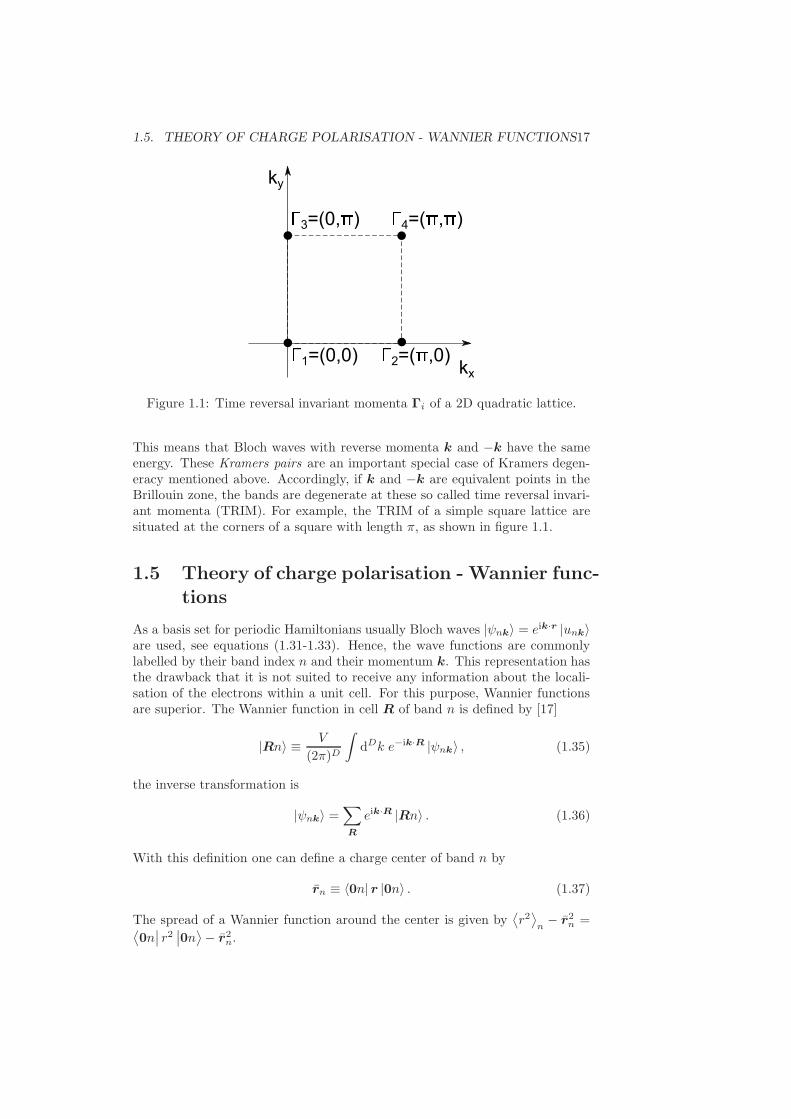
Figure 1.1: Time reversal invariant momenta Γi of a 2D quadratic lattice.
This means that Bloch waves with reverse momenta k and −k have the sameenergy. These Kramers pairs are an important special case of Kramers degen-eracy mentioned above. Accordingly, if k and −k are equivalent points in theBrillouin zone, the bands are degenerate at these so called time reversal invari-ant momenta (TRIM). For example, the TRIM of a simple square lattice aresituated at the corners of a square with length π, as shown in figure 1.1.
1.5 Theory of charge polarisation - Wannier func-
tions
As a basis set for periodic Hamiltonians usually Bloch waves |ψnk〉 = eik·r |unk〉are used, see equations (1.31-1.33). Hence, the wave functions are commonlylabelled by their band index n and their momentum k. This representation hasthe drawback that it is not suited to receive any information about the locali-sation of the electrons within a unit cell. For this purpose, Wannier functionsare superior. The Wannier function in cell R of band n is defined by [17]
|Rn〉 ≡ V
(2π)D
∫dDk e−ik·R |ψnk〉 , (1.35)
the inverse transformation is
|ψnk〉 =∑
R
eik·R |Rn〉 . (1.36)
With this definition one can define a charge center of band n by
rn ≡ 〈0n| r |0n〉 . (1.37)
The spread of a Wannier function around the center is given by⟨r2⟩n− r2
n =⟨0n∣∣ r2
∣∣0n⟩− r2
n.
18 CHAPTER 1. TOPOLOGICAL INVARIANTS
The connection of Wannier functions to topology is due to a relation pre-sented in [18], which links matrix elements of the position operator in the Wan-nier basis to the Berry connection An(k) = −i 〈unk| ∇k |uvk〉:
〈Rn| r |0m〉 = iV
(2π)3
∫d3k eik·R 〈unk| ∇k |umk〉 . (1.38)
With this expression one can easily formulate the charge center as well as thespread in terms of Bloch functions |unk〉 [19]:
rn = iV
(2π)3
∫d3k 〈unk| ∇k |unk〉 (1.39)
⟨r2⟩n=
V
(2π)3
∫d3k |∇k |unk〉|2 (1.40)
However, the definition of all quantities above is not unique since the Blochfunctions associated with the Wannier functions have a gauge freedom. Onecan modify the basis function by a phase
|unk〉 → eiφn(k) |unk〉 (1.41)
and still preserve a valid set of Bloch functions. The Wannier center rn remainsthe same, modulo a lattice vector, whereas the spread changes [19]. In general,one can transform not only a single Bloch function, but also a set of Blochfunctions using a unitary matrix Umn:
|unk〉 →∑
m
Umn(k) |umk〉 . (1.42)
The new set of vectors |unk〉 are not necessarily eigenvectors of H(k) as definedin equation (1.33) any more but span still the whole space. Furthermore, thegeneralized gauge transformation changes also the Wannier charge centers rn,the only quantity preserved (up to a lattice vector) is the total charge center∑
n rn.
1.6 Definition of Z2 invariant by Fu and Kane
In their original work [20] Fu and Kane considered a one dimensional periodicHamiltonian H with a lattice constant a = 1, length L and periodic boundaryconditions. Furthermore, H changes adiabatically with a pumping parameter t.This parameter is periodic with period T
H [t+ T ] = H [t] (1.43)
and odd under time reversal Θ
H [−t] = ΘH [t]Θ−1. (1.44)
The idea is now to use Wannier charge centers (WCCs) to describe thetopological properties of this system, since the expression for charge centers(1.39) is proportional to a Berry phase (1.5). In our 1D case, the expression fora polarisation Pn reads
Pn ≡ 〈0n|x |0n〉 = i
2π
∫ π
−π
dk 〈unk| ∂k |unk〉 = Cn (1.45)
1.6. DEFINITION OF Z2 INVARIANT BY FU AND KANE 19
k0 ππ
α=1
α=2
α=3
II
I
II
II
I
I
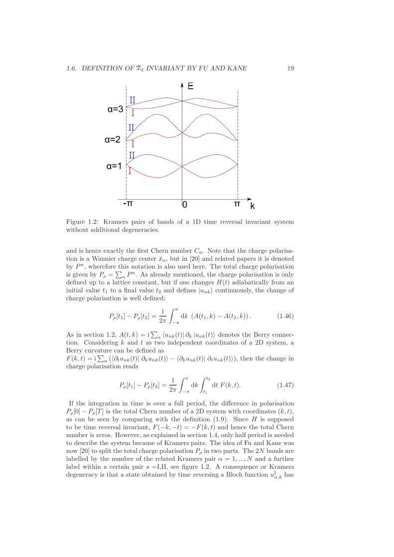
Figure 1.2: Kramers pairs of bands of a 1D time reversal invariant systemwithout additional degeneracies.
and is hence exactly the first Chern number Cn. Note that the charge polarisa-tion is a Wannier charge center xn, but in [20] and related papers it is denotedby Pn, wherefore this notation is also used here. The total charge polarisationis given by Pρ =
∑n P
n. As already mentioned, the charge polarisation is onlydefined up to a lattice constant, but if one changes H(t) adiabatically from aninitial value t1 to a final value t2 and defines |unk〉 continuously, the change ofcharge polarisation is well defined:
Pρ[t1]− Pρ[t2] =1
2π
∫ π
−π
dk (A(t1, k)−A(t2, k)) . (1.46)
As in section 1.2, A(t, k) = i∑
n 〈unk(t)| ∂k |unk(t)〉 denotes the Berry connec-tion. Considering k and t as two independent coordinates of a 2D system, aBerry curvature can be defined asF (k, t) = i
∑n (〈∂tunk(t)| ∂kunk(t)〉 − 〈∂kunk(t)| ∂tunk(t)〉), then the change in
charge polarisation reads
Pρ[t1]− Pρ[t2] =1
2π
∫ π
−π
dk
∫ t2
t1
dt F (k, t). (1.47)
If the integration in time is over a full period, the difference in polarisationPρ[0]−Pρ[T ] is the total Chern number of a 2D system with coordinates (k, t),as can be seen by comparing with the definition (1.9). Since H is supposedto be time reversal invariant, F (−k,−t) = −F (k, t) and hence the total Chernnumber is zeros. However, as explained in section 1.4, only half period is neededto describe the system because of Kramers pairs. The idea of Fu and Kane wasnow [20] to split the total charge polarisation Pρ in two parts. The 2N bands arelabelled by the number of the related Kramers pair α = 1, ..., N and a furtherlabel within a certain pair s =I,II, see figure 1.2. A consequence or Kramersdegeneracy is that a state obtained by time reversing a Bloch function uIα,k has
20 CHAPTER 1. TOPOLOGICAL INVARIANTS
to be, up to a phase χα,k, its Kramers partner uIIα,−k. The Bloch waves withina band are thus related by
∣∣uIα,−k
⟩= −eiχα,kΘ
∣∣uIIα,k⟩
(1.48)∣∣uIIα,−k
⟩= eiχα,−kΘ
∣∣uIα,k⟩. (1.49)
The second equation follows from the first and the properties of the time reversaloperator. The splitting of the Kramers pairs allows the definition of partialpolarisations P I and P II given by
P s =1
2π
∫ π
−π
dk As(k), (1.50)
As(k) = iN∑
α=1
〈usαk|∂k |usαk〉 . (1.51)
Obviously, the total charge polarisation is the sum of the two partial polarisa-tions Pρ = P I +P II. For the definition of the Z2 invariant, the difference of thepartial polarisations, called time reversal polarisation
Pθ ≡ P I − P II (1.52)
is needed. Taking the time reversal invariance into consideration, integratingover half a period is sufficient to determine properties of the system. The Z2
invariant for time reversal invariant systems is thus defined by
ν ≡ Pθ[T/2]− Pθ[0] mod 2. (1.53)
In the same paper [20], Fu and Kane also presented a method to determinethe invariant. The method is not used in this thesis, but it is explained forcompleteness. The most important quantities for that purpose are the overlapmatrices of time reversed Bloch states
wmn(k) = 〈um,−k|Θ |un,k〉 . (1.54)
Because of equation (1.48), w(k) are direct products of 2×2 matrices where theoff-diagonal elements are the complex phases eiχα,k and eiχα,−k . Especially, inthe case of the two time reversal invariant momenta (TRIM) k = 0 and k = π,the matrices w(k) are antisymmetric. Remarkably, it can be shown [20] thatonly the time reversal overlap matrices at k = 0, π and t = 0, T/2 arenecessary to determine the Z2 invariant. These four momentum/time pairs aredenoted Γi and the invariant can be calculated from
(−1)ν =
4∏
i=1
δi with δi =
√det[w(Γi)]
Pf[w(Γi)]. (1.55)
Since the Pfaffian Pf, which is only defined for antisymmetric matrices as it isthe case for w(Γi), is the square root of the determinant, only the branch of thesquare root in equation (1.55) determines the sign of δi. The branch has to bechosen such that the |unk〉 as well as
√det[w(k)] are continuous between k = 0
and k = π. To implement a local gauge satisfying this is the most challenging
1.7. SOLUYANOV-VANDERBILT METHOD 21
part of this method.
The motivation here was given for a 1D system depending on an adiabaticpumping parameter t. For two-dimensional systems the Z2 invariant can bedefined and calculated similarly, one just has to identify the momentum in thesecond direction ky as the pumping parameter, thus all quantities depend on(kx, ky) instead of (k, t). Equation (1.55) is still valid, Γi are the TRIM (0, 0),
(0, π), (π, 0) and (π, π) (see figure 1.1). The continuity of |unk〉 and√det[w(k)]
has to be satisfied along two opposing edges of the square defined by the fourTRIM, so either from (0, 0) to (0, π) and from (π, 0) and (π, π), or from (0, 0)to (π, 0) and from (0, π) to (π, π).
1.6.1 Topological systems with inversion symmetry
As mentioned above, to use equation (1.55) a local gauge has to be used such thatthe eigenstates are continuous between the TRIM. Fortunately, for the specialcase of Hamiltonians with inversion symmetry it is possible to reformulate thisequation so that no knowledge of the eigenstates between the TRIM is necessary.
Inversion symmetry means that mirroring the lattice at an inversion center ileaves the Hamiltonian invariant. Usually, i defines the origin O of the unit cellwhich means inversion is realized by the parity operation P which maps all vec-tors in real space to its negative, i.e. P : x 7→ −x. If a Hamiltonian is inversionsymmetric, the Bloch matrix H(k) commutes with a matrix representation Pof the parity transformation P . Thus, a complete set of common eigenvectorsexists [21]. The Bloch functions |unk〉 are therefore eigenfunctions of the parityoperator P with eigenvalues ξn = ±1.
If the Hamiltonian is furthermore time reversal invariant, the eigenfunctionscan be divided in Kramers pairs (see section 1.4). The parity eigenvalue ofeigenfunctions belonging to the same Kamers pair are equal ξIα = ξIIα = ξα [22].It can be shown that the Z2 invariant is given just by the eigenvalues ξα of theparity operator of the Kramers pair α at the TRIM Γi [22].
(−1)ν =
4∏
i=1
δi with δi =
N∏
α=1
ξα(Γi) (1.56)
The calculation of δi is here much simpler than in the more general equation(1.55) since no continuous gauge between the TRIM has to be found.
1.7 Soluyanov-Vanderbilt method to determine
the Z2 invariant
The method described in this section was first published by Soluyanov andVanderbilt [23] and is based on definition (1.53). Since in this thesis onlytwo-dimensional systems where ky plays the role of the pumping parametert are considered, I use in this section only the notation (kx, ky) rather than theparametrisation (k, t) which is used in section 1.6 and the original papers [20]
22 CHAPTER 1. TOPOLOGICAL INVARIANTS
and [23].
In this 2D parametrisation the Wannier functions of interest are the hybridWannier functions where in contrast to definition (1.35) only one coordinate istransformed from momentum k to spacial coordinates,
|Rxkyn〉 =1
2π
∫ π
−π
dkx e−iRxkx |ψnk〉 . (1.57)
The Wannier charge center (WCC) is thus the expectation value of the x com-ponent of the position operator and depends on ky,
xn(ky) =⟨0kyn
∣∣∣ X∣∣∣0kyn
⟩. (1.58)
From equation (1.39) it follows that the WCC can also be written as
xn(ky) =i
2π
∫ π
−π
dkx 〈unk| ∂kx|unk〉 (1.59)
which is the polarisation in x direction, see equation (1.45). Hence, the Z2
invariant defined by equation (1.55) can also be written as
ν =∑
α
[xIα(π) − xIIα (π)
]−∑
α
[xIα(0)− xIIα (0)
](1.60)
where α labels again the Kramers pair and (I,II) the number within a pair, seefigure 1.2. Because of Kramers degeneracy, xIα = xIIα modulo a lattice constantat ky = 0 and ky = π. Therefore, each of the summands in equation (1.60) isan integer. However, to find the correct integer, the branch of xn(k) must notchange evolving from ky = 0 to ky = π.
The hybrid Wannier functions are not uniquely defined as explained in sec-tion 1.5, since the bands still have the freedom of unitary gauge transformations
|umk〉 =∑
n
Umn(k) |unk〉 . (1.61)
The desired gauge that makes sure that the correct branches are chosen is thegauge that leads to maximally localised Wannier charge centers, as long as theWCCs evolve smoothly [23]. The maximally localised WCC is defined as theWCC with the minimal total spread [19]
Ω =∑
n
[⟨0kyn
∣∣∣ X2∣∣∣0kyn
⟩−⟨0kyn
∣∣∣ X∣∣∣0kyn
⟩2]. (1.62)
This condition defines a local gauge where the unitary transformation matrixU(k) can be calculated using the following recipe for each value of ky [19, 23].
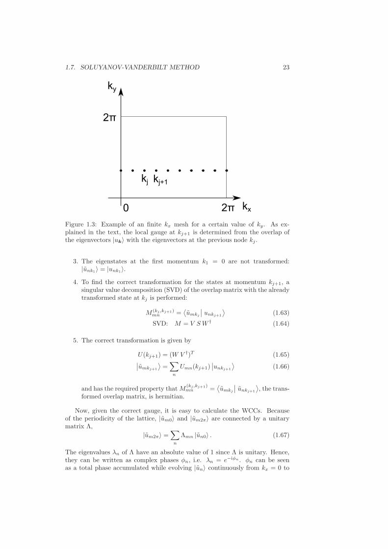
1. Define a discrete mesh of points k1, ..., kN along kx, see figure 1.3. I used,as recommended by Soluyanov and Vanderbilt, 10 nodes.
2. For all of the discrete points, calculate the eigenvectors∣∣unkj
⟩.
1.7. SOLUYANOV-VANDERBILT METHOD 23
kx
ky
0 2π
2π
kj kj+1
Figure 1.3: Example of an finite kx mesh for a certain value of ky. As ex-plained in the text, the local gauge at kj+1 is determined from the overlap ofthe eigenvectors |uk〉 with the eigenvectors at the previous node kj .
3. The eigenstates at the first momentum k1 = 0 are not transformed:|unk1
〉 = |unk1〉.
4. To find the correct transformation for the states at momentum kj+1, asingular value decomposition (SVD) of the overlap matrix with the alreadytransformed state at kj is performed:
M (kj ,kj+1)mn =
⟨umkj
∣∣ unkj+1
⟩(1.63)
SVD: M = V SW † (1.64)
5. The correct transformation is given by
U(kj+1) = (W V †)T (1.65)∣∣umkj+1
⟩=∑
n
Umn(kj+1)∣∣unkj+1
⟩(1.66)
and has the required property thatM(kj,kj+1)mn =
⟨umkj
∣∣ unkj+1
⟩, the trans-
formed overlap matrix, is hermitian.
Now, given the correct gauge, it is easy to calculate the WCCs. Becauseof the periodicity of the lattice, |um0〉 and |um2π〉 are connected by a unitarymatrix Λ,
|um2π〉 =∑
n
Λmn |un0〉 . (1.67)
The eigenvalues λn of Λ have an absolute value of 1 since Λ is unitary. Hence,they can be written as complex phases φn, i.e. λn = e−iφn . φn can be seenas a total phase accumulated while evolving |un〉 continuously from kx = 0 to
24 CHAPTER 1. TOPOLOGICAL INVARIANTS
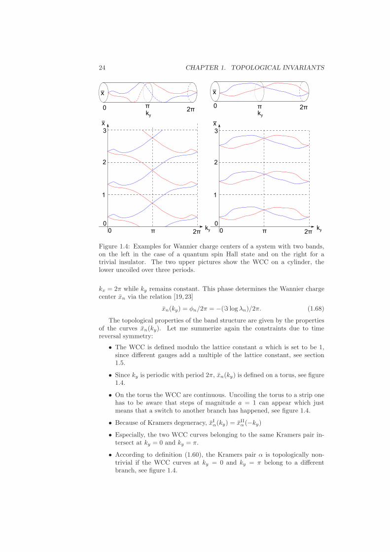
Figure 1.4: Examples for Wannier charge centers of a system with two bands,on the left in the case of a quantum spin Hall state and on the right for atrivial insulator. The two upper pictures show the WCC on a cylinder, thelower uncoiled over three periods.
kx = 2π while ky remains constant. This phase determines the Wannier chargecenter xn via the relation [19, 23]
xn(ky) = φn/2π = −(ℑ logλn)/2π. (1.68)
The topological properties of the band structure are given by the propertiesof the curves xn(ky). Let me summerize again the constraints due to timereversal symmetry:
• The WCC is defined modulo the lattice constant a which is set to be 1,since different gauges add a multiple of the lattice constant, see section1.5.
• Since ky is periodic with period 2π, xn(ky) is defined on a torus, see figure1.4.
• On the torus the WCC are continuous. Uncoiling the torus to a strip onehas to be aware that steps of magnitude a = 1 can appear which justmeans that a switch to another branch has happened, see figure 1.4.
• Because of Kramers degeneracy, xIα(ky) = xIIα (−ky)• Especially, the two WCC curves belonging to the same Kramers pair in-tersect at ky = 0 and ky = π.
• According to definition (1.60), the Kramers pair α is topologically non-trivial if the WCC curves at ky = 0 and ky = π belong to a differentbranch, see figure 1.4.
1.8. TOPOLOGICAL INVARIANTS FOR INTERACTING SYSTEMS 25
0 0.5 1 1.5 2−0.5
0
0.5
1
1.5
x
ky/π0 0.5 1 1.5 2
−0.5
0
0.5
1
1.5
x
ky/π
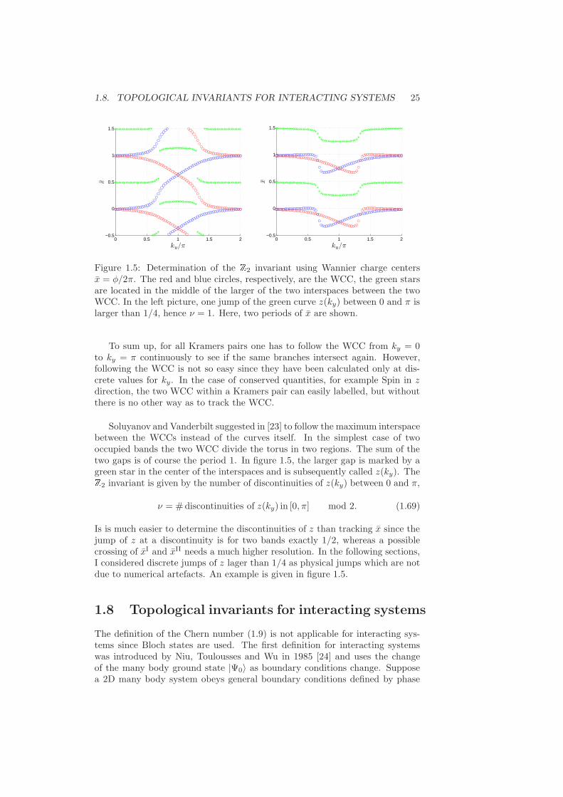
Figure 1.5: Determination of the Z2 invariant using Wannier charge centersx = φ/2π. The red and blue circles, respectively, are the WCC, the green starsare located in the middle of the larger of the two interspaces between the twoWCC. In the left picture, one jump of the green curve z(ky) between 0 and π islarger than 1/4, hence ν = 1. Here, two periods of x are shown.
To sum up, for all Kramers pairs one has to follow the WCC from ky = 0to ky = π continuously to see if the same branches intersect again. However,following the WCC is not so easy since they have been calculated only at dis-crete values for ky. In the case of conserved quantities, for example Spin in zdirection, the two WCC within a Kramers pair can easily labelled, but withoutthere is no other way as to track the WCC.
Soluyanov and Vanderbilt suggested in [23] to follow the maximum interspacebetween the WCCs instead of the curves itself. In the simplest case of twooccupied bands the two WCC divide the torus in two regions. The sum of thetwo gaps is of course the period 1. In figure 1.5, the larger gap is marked by agreen star in the center of the interspaces and is subsequently called z(ky). TheZ2 invariant is given by the number of discontinuities of z(ky) between 0 and π,
ν = #discontinuities of z(ky) in [0, π] mod 2. (1.69)
Is is much easier to determine the discontinuities of z than tracking x since thejump of z at a discontinuity is for two bands exactly 1/2, whereas a possiblecrossing of xI and xII needs a much higher resolution. In the following sections,I considered discrete jumps of z lager than 1/4 as physical jumps which are notdue to numerical artefacts. An example is given in figure 1.5.
1.8 Topological invariants for interacting systems
The definition of the Chern number (1.9) is not applicable for interacting sys-tems since Bloch states are used. The first definition for interacting systemswas introduced by Niu, Toulousses and Wu in 1985 [24] and uses the changeof the many body ground state |Ψ0〉 as boundary conditions change. Supposea 2D many body system obeys general boundary conditions defined by phase
26 CHAPTER 1. TOPOLOGICAL INVARIANTS
shifts φx, φy which impose
Ψ0(. . . , xi + nxLx, yi + nyLy, . . . ) = ei(nxφx+nyφy)Ψ0(. . . , xi, yi, . . . ).
The Chern number of the system is then given by [13, 24]
C =
∫ 2π
0
∫ 2π
0
dφxdφy2πi
(⟨∂Ψ0
∂φy
∣∣∣∣∂Ψ0
∂φx
⟩−⟨∂Ψ0
∂φx
∣∣∣∣∂Ψ0
∂φy
⟩). (1.70)
For a Z2 invariant or a spin Chern number, the phase shift might be different forspin up and spin down variables. Thus, the Chern number for each combinationhas to be calculated via [13, 15]
Cσσ′
=
∫ 2π
0
∫ 2π
0
dφσxdφσ′
y
2πi
(⟨∂Ψ0
∂φσ′
y
∣∣∣∣∂Ψ0
∂φσx
⟩−⟨∂Ψ0
∂φσx
∣∣∣∣∂Ψ0
∂φσ′
y
⟩). (1.71)
The total Chern number is given by C =∑
σσ′ Cσσ′and the spin Chern number
in analogy to (1.27) by C =∑
σσ′ σ Cσσ′[13, 15].
In most cases, this expressions are difficult to evaluate. However, informationabout some quantum mechanical many body system is not only given by themany body ground state, but also by the Green’s function. Fortunately, is ispossible to reformulate equation (1.70) in terms of the single particle Green’sfunction [24–26]
C =ǫµνρ
24π2
∫dk0
∫d2k Tr
[G∂µG
−1G∂νG−1G∂ρG
−1]
(1.72)
where k0 is the real frequency k0 ≡ ω ∈ R and G = G(iω,k) the Green’s func-tion in Matsubara representation. G is a matrix whose indices are the remainingdegrees of freedom after translational invariance has been used to transform tomomentum space k, as for example spin and different sites within a unit cell,and G−1 denotes the matrix inverse of G. Furthermore, ∂µ ≡ ∂
∂kµand Greek
letters are looping from 0 to 3, i.e. µ = 0, 1, 2, 3, where the Einstein conventionof implicit summation is used. This formulation using Green’s functions givesqualitative information about topology, for example, a change of the topologicalinvariant can only happen if a singularity appears in G or G−1 [25,27]. However,the numerical evaluation of (1.72) is demanding since a good knowledge of thederivatives of the Green’s function is necessary to compute the triple integralaccurately.
A huge simplification could be achieved by Zhong Wang et al. developinga new method where the Green’s function is only needed at frequency ω = 0[28–30]. We can introduce an equation of the Green’s function at ω = 0 whichreads
G−1(ω = 0,k) |α(ω = 0,k)〉 = µα(ω = 0,k) |α(ω = 0,k)〉 . (1.73)
It is possible to calculate a quantity
Cα =1
2π
∫
BZ
d2k ·Fα(k) =1
2π
∮
∂BZ
dk ·Aα(k), (1.74)
1.9. BULK BOUNDARY CORRESPONDENCE 27
with Fα(k) = ∇k × Aα(k) and Aα(k) = −i 〈α(0,k)| ∇k |α(0,k)〉, directlyfrom the eigenvectors of G−1. These quantities are Chern numbers and thusinteger valued since they have the same structure as the Chern number definedfor noninteracting systems (1.9). The difference is that another vector bundle isused: Instead of Bloch states |u(k)〉 which define the topology of the band Chernnumbers through Berry connections Am(k) = i 〈umk| ∇k |umk〉, eigenfunctions|α(k)〉 of G−1(ω = 0,k) define the topology of these different Chern numbersthrough Berry connections Aα(k) = −i 〈α(0,k)| ∇k |α(0,k)〉. On the first sight,invariants defined on different bundles may not be connected in any way, butit is the remarkable work of Wang et al. to show that summing over all Cα
belonging to positive eigenvalues µα > 0 (usually called R-space in contrast toL-space witch is the space of vectors with negative eigenvalues) gives exactlythe same total Chern invariant as defined by (1.72),
C =∑
α∈R-space
Cα. (1.75)
If the system obeys inversion symmetry, G−1(ω,k) commutes at the TRIM k =Γi with the parity transformation matrix P (see also section 1.6.1) wherefore|α(ω,Γi)〉 are simultaneous eigenstates of G and P :
P |α(ω = 0,Γi)〉 = ηα |α(ω = 0,Γi)〉 . (1.76)
In [28] it is shown that the topological invariant can be calculated from theseeigenvalues trough
(−1)ν =∑
R zeros
η1/2α (1.77)
and that it reduces to the Fu-Kane formula (1.56) in the noninteracting case.Here, the convention (−1)1/2 = i is used.
To sum up, one can calculate the desired Chern invariant by evaluating Berryphases related to eigenvectors with positive eigenvalues of the inverse Green’sfunction matrix G−1(ω = 0,k). One the other hand, for noninteracting systems,the Chern invariant is calculated using eigenvectors with negative eigenvalues ofa matrix H(k). Hence, the topological properties of an interacting system arethe same as for an artificial noninteracting Bloch Hamiltonian which is minusthe inverse Green’s function at ω = 0. This defines the so called topologicalHamiltonian
Ht(k) = −G−1(ω = 0,k). (1.78)
Thus, all topological properties are encoded in an artificial system. Since thisis interactionless, all methods described in the previous sections can be usedto calculate the Chern invariant. However, it is prudent to mention that onlythe topological properties are encoded in Ht(k), it is not suitable to use it forestimates of any other quantities.
1.9 Bulk boundary correspondence
A fundamental aspect of finite topological systems is the appearance of gaplessstates at the boundary, for example 1D states at the edge of a 2D ribbon. The
28 CHAPTER 1. TOPOLOGICAL INVARIANTS
basic idea behind this correspondence between the topologically nontrivial bulkand the existence of gapless states at the boundary is the stability of topologicalinvariants with respect to minor modifications of the bands. As mentioned insection 1.2, the Chern number can only change if a gap closes and a quantumphase transition happens. A boundary can be seen now as a sharp change ofthe Hamiltonian from a topologically nontrivial system to the vacuum, which istopologically trivial (the bands are the dispersions of free electrons and positronsas conduction band and valence band, respectively). The change of a topolog-ical invariant involves, as mentioned above, a gap closing which has to happenexactly at the boundary.
Such edge states have already be found by Jackiw and Rebbi in 1976 [31] andreappear in the model by Su, Schrieffer and Heeger [32]. The idea from Jackiwand Rebbi of an 1D field theory with edge states is used in the review by Hasanand Kane [7] as an introductory example to bulk boundary correspondence. Themodel is a Hamiltonian of massive Dirac particles living on a honeycomb lattice(Details on that lattice are explained later in section 2.1). For small momentaaround the K points, q ≡ k −K and mass m the Hamiltonian reads
H(q) = ~vF q · σ +mσz (1.79)
and has the energies E(q) = ±√|~vFq|2 +m2 with a gap of 2 |m|. If m has
a different sign at the two K points K and K ′, the system is a topologicalinsulator, otherwise a trivial insulator. Consider now an interface where thesign of m at K ′ is changing as a function of y as m(y) = |m|Θ(y) (Θ is theHeaviside step function), but remains positive at K. The Schrodinger equationhas then the simple solution
ψqx(x, y) ∝ eiqxx−∫
y
0dy′ m(y′)/vF
(1
1
)(1.80)
with the linear dispersion E(qx) = ~vF qx. Hence, there exists a gapless edgestate exponentially localized at the interface.
Analysing the eigenfunctions of a Hamiltonian has been also considered atquantum Hall insulators by Halperin [33] shortly after the experimental discov-ery of the QH effect even before TKNN published their theoretical description.Halperin’s paper is based on the idea of Laughlin, who has shown the quanti-sation of Hall conductivity by using gauge invariance and a mobility gap [34].The geometry used by Laughlin is a metal ring pierced by a magnetic fieldH0. Through the ring flows a variable magnetic flux Φ, see figure 1.6. TheHamiltonian of that system with charge carriers of mass m∗ is
H =~2
2m∗
(P − e
cA)2
+ eE0y. (1.81)
With a Landau gauge for the magnetic field A = H0yx the Landau levels En =(n+ 1
2
)~ωc with the cyclotron frequency ωc = |eB0| /m∗c can be proven. In his
gedankenexperiment, Laughlin changed the vector potential to A → A + A0xwhich physically means turning on a magnetic flux Φ = A0Lx through the loop
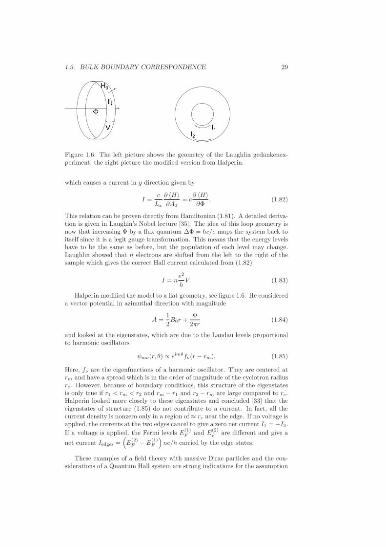
1.9. BULK BOUNDARY CORRESPONDENCE 29
H0
1
2
Figure 1.6: The left picture shows the geometry of the Laughlin gedankenex-periment, the right picture the modified version from Halperin.
which causes a current in y direction given by
I =c
Lx
∂ 〈H〉∂A0
= c∂ 〈H〉∂Φ
. (1.82)
This relation can be proven directly from Hamiltonian (1.81). A detailed deriva-tion is given in Laughin’s Nobel lecture [35]. The idea of this loop geometry isnow that increasing Φ by a flux quantum ∆Φ = hc/e maps the system back toitself since it is a legit gauge transformation. This means that the energy levelshave to be the same as before, but the population of each level may change.Laughlin showed that n electrons are shifted from the left to the right of thesample which gives the correct Hall current calculated from (1.82)
I = ne2
hV. (1.83)
Halperin modified the model to a flat geometry, see figure 1.6. He considereda vector potential in azimuthal direction with magnitude
A =1
2B0r +
Φ
2πr(1.84)
and looked at the eigenstates, which are due to the Landau levels proportionalto harmonic oscillators
ψmν(r, θ) ∝ eimθfν(r − rm). (1.85)
Here, fν are the eigenfunctions of a harmonic oscillator. They are centered atrm and have a spread which is in the order of magnitude of the cyclotron radiusrc. However, because of boundary conditions, this structure of the eigenstatesis only true if r1 < rm < r2 and rm − r1 and r2 − rm are large compared to rc.Halperin looked more closely to these eigenstates and concluded [33] that theeigenstates of structure (1.85) do not contribute to a current. In fact, all thecurrent density is nonzero only in a region of ≈ rc near the edge. If no voltage isapplied, the currents at the two edges cancel to give a zero net current I1 = −I2.If a voltage is applied, the Fermi levels E
(1)F and E
(2)F are different and give a
net current Iedges =(E
(2)F − E
(1)F
)ne/h carried by the edge states.
These examples of a field theory with massive Dirac particles and the con-siderations of a Quantum Hall system are strong indications for the assumption
30 CHAPTER 1. TOPOLOGICAL INVARIANTS
stated at the beginning of this section that a surface or an interface betweentwo materials with different topological properties accompanies edge states. Formany systems, rigorous proofs exist. Essin and Gurarie have shown in [27] thatthe existence of edge states follows from the a nonzero topological invariantgiven in terms of Green’s functions (see equation (1.72)). This approach is verygeneral and valid for all 10 topological classes in all dimensions and uses the factthat a Chern integer defined by (1.72) can only change if the Green’s functionhas a pole or a zero. The proof presumes that no Green’s function zeros appear,which is true if the system is noninteracting. For interacting systems, Green’sfunction zeros can appear and hence it is in principle possible that no edgestates are at an interface between two interacting topological insulators, whichhence can be continuously deformed from one to another without ever closingthe bulk gap [25]. The Chern number in terms of Green’s functions (1.72) is de-signed such that it adiabatically connected to Chern numbers of noninteractingsystems calculated from Bloch functions. It thus has the right properties in thelimit of vanishing interaction, but its meaning for strongly interacting systemsis still not clear [13].
Another interesting proof is from Schulz-Baldes [36] who has shown for 2Dsystems with time-reversal symmetry breaking terms, as for example Rashbaspin-orbit, that the spin edge currents persist provided there is a spectral gapand the spin Chern numbers (1.27) are nontrivial. Graf and Porta [37], on theother hand, give a new definition of the Z2 invariant for both bulk and edgeand show that these are equivalent.
Chapter 2
The Kane-Mele model
2.1 Graphene
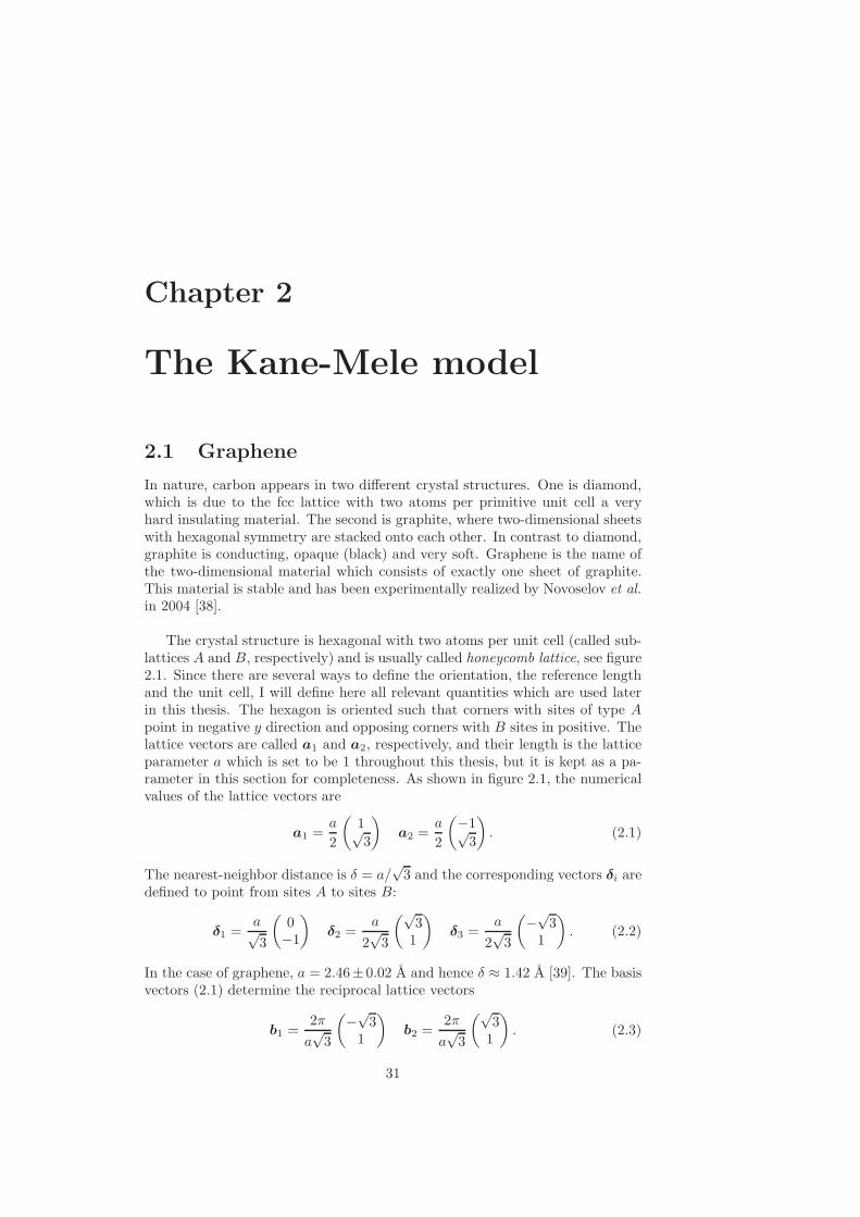
In nature, carbon appears in two different crystal structures. One is diamond,which is due to the fcc lattice with two atoms per primitive unit cell a veryhard insulating material. The second is graphite, where two-dimensional sheetswith hexagonal symmetry are stacked onto each other. In contrast to diamond,graphite is conducting, opaque (black) and very soft. Graphene is the name ofthe two-dimensional material which consists of exactly one sheet of graphite.This material is stable and has been experimentally realized by Novoselov et al.in 2004 [38].
The crystal structure is hexagonal with two atoms per unit cell (called sub-lattices A and B, respectively) and is usually called honeycomb lattice, see figure2.1. Since there are several ways to define the orientation, the reference lengthand the unit cell, I will define here all relevant quantities which are used laterin this thesis. The hexagon is oriented such that corners with sites of type Apoint in negative y direction and opposing corners with B sites in positive. Thelattice vectors are called a1 and a2, respectively, and their length is the latticeparameter a which is set to be 1 throughout this thesis, but it is kept as a pa-rameter in this section for completeness. As shown in figure 2.1, the numericalvalues of the lattice vectors are
a1 =a
2
(1√3
)a2 =
a
2
(−1√3
). (2.1)
The nearest-neighbor distance is δ = a/√3 and the corresponding vectors δi are
defined to point from sites A to sites B:
δ1 =a√3
(0−1
)δ2 =
a
2√3
(√31
)δ3 =
a
2√3
(−√3
1
). (2.2)
In the case of graphene, a = 2.46± 0.02 A and hence δ ≈ 1.42 A [39]. The basisvectors (2.1) determine the reciprocal lattice vectors
b1 =2π
a√3
(−√3
1
)b2 =
2π
a√3
(√31
). (2.3)
31
32 CHAPTER 2. THE KANE-MELE MODEL
Figure 2.1: Honeycomb lattice in real space. Full circles represent sublatticeA, empty circles sublattice B. The primitive lattice vectors ai are defined inequation (2.1), the nearest-neighbor vectors δi in equation (2.2).
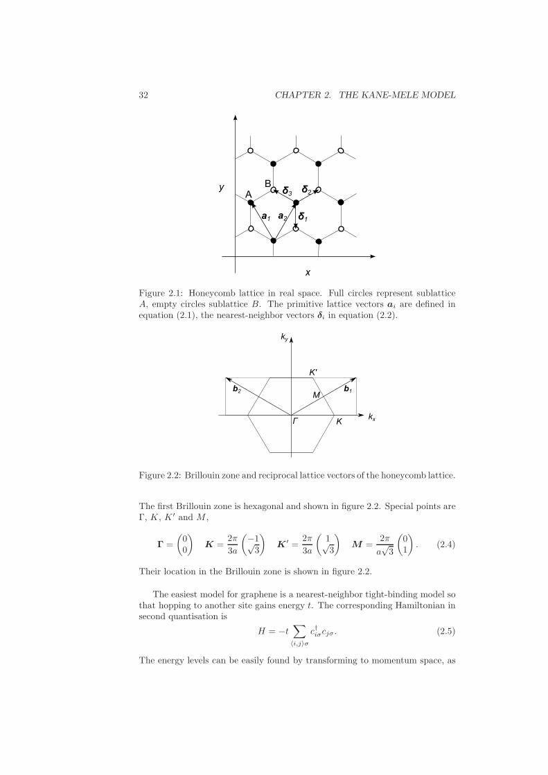
Figure 2.2: Brillouin zone and reciprocal lattice vectors of the honeycomb lattice.
The first Brillouin zone is hexagonal and shown in figure 2.2. Special points areΓ, K, K ′ and M ,
Γ =
(00
)K =
2π
3a
(−1√3
)K ′ =
2π
3a
(1√3
)M =
2π
a√3
(01
). (2.4)
Their location in the Brillouin zone is shown in figure 2.2.
The easiest model for graphene is a nearest-neighbor tight-binding model sothat hopping to another site gains energy t. The corresponding Hamiltonian insecond quantisation is
H = −t∑
〈i,j〉σc†iσcjσ . (2.5)
The energy levels can be easily found by transforming to momentum space, as
2.1. GRAPHENE 33
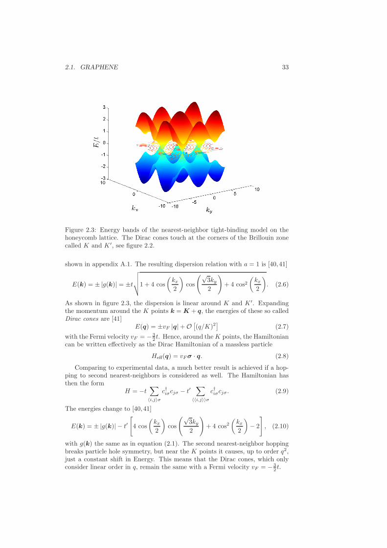
Figure 2.3: Energy bands of the nearest-neighbor tight-binding model on thehoneycomb lattice. The Dirac cones touch at the corners of the Brillouin zonecalled K and K ′, see figure 2.2.
shown in appendix A.1. The resulting dispersion relation with a = 1 is [40, 41]
E(k) = ± |g(k)| = ±t
√√√√1 + 4 cos
(kx2
)cos
(√3ky2
)+ 4 cos2
(kx2
). (2.6)
As shown in figure 2.3, the dispersion is linear around K and K ′. Expandingthe momentum around the K points k = K + q, the energies of these so calledDirac cones are [41]
E(q) = ±vF |q|+O[(q/K)2
](2.7)
with the Fermi velocity vF = − 32 t. Hence, around theK points, the Hamiltonian
can be written effectively as the Dirac Hamiltonian of a massless particle
Heff(q) = vFσ · q. (2.8)
Comparing to experimental data, a much better result is achieved if a hop-ping to second nearest-neighbors is considered as well. The Hamiltonian hasthen the form
H = −t∑
〈i,j〉σc†iσcjσ − t′
∑
〈〈i,j〉〉σc†iσcjσ. (2.9)
The energies change to [40, 41]
E(k) = ± |g(k)| − t′[4 cos
(kx2
)cos
(√3ky2
)+ 4 cos2
(kx2
)− 2
], (2.10)
with g(k) the same as in equation (2.1). The second nearest-neighbor hoppingbreaks particle hole symmetry, but near the K points it causes, up to order q2,just a constant shift in Energy. This means that the Dirac cones, which onlyconsider linear order in q, remain the same with a Fermi velocity vF = − 3
2 t.
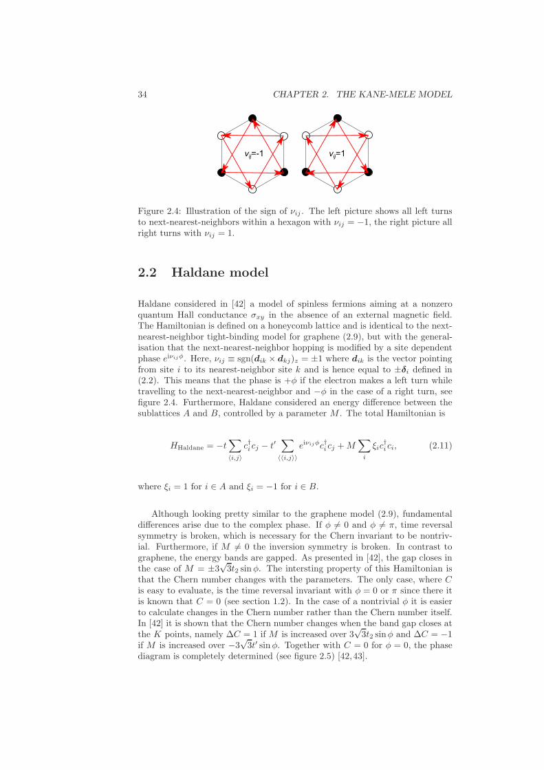
34 CHAPTER 2. THE KANE-MELE MODEL
Figure 2.4: Illustration of the sign of νij . The left picture shows all left turnsto next-nearest-neighbors within a hexagon with νij = −1, the right picture allright turns with νij = 1.
2.2 Haldane model
Haldane considered in [42] a model of spinless fermions aiming at a nonzeroquantum Hall conductance σxy in the absence of an external magnetic field.The Hamiltonian is defined on a honeycomb lattice and is identical to the next-nearest-neighbor tight-binding model for graphene (2.9), but with the general-isation that the next-nearest-neighbor hopping is modified by a site dependentphase eiνijφ. Here, νij ≡ sgn(dik × dkj)z = ±1 where dik is the vector pointingfrom site i to its nearest-neighbor site k and is hence equal to ±δi defined in(2.2). This means that the phase is +φ if the electron makes a left turn whiletravelling to the next-nearest-neighbor and −φ in the case of a right turn, seefigure 2.4. Furthermore, Haldane considered an energy difference between thesublattices A and B, controlled by a parameter M . The total Hamiltonian is
HHaldane = −t∑
〈i,j〉c†i cj − t′
∑
〈〈i,j〉〉eiνijφc†i cj +M
∑
i
ξic†i ci, (2.11)
where ξi = 1 for i ∈ A and ξi = −1 for i ∈ B.
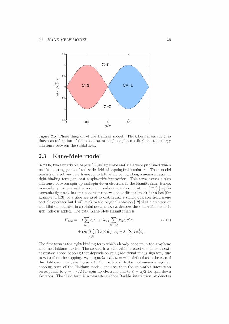
Although looking pretty similar to the graphene model (2.9), fundamentaldifferences arise due to the complex phase. If φ 6= 0 and φ 6= π, time reversalsymmetry is broken, which is necessary for the Chern invariant to be nontriv-ial. Furthermore, if M 6= 0 the inversion symmetry is broken. In contrast tographene, the energy bands are gapped. As presented in [42], the gap closes inthe case of M = ±3
√3t2 sinφ. The intersting property of this Hamiltonian is
that the Chern number changes with the parameters. The only case, where Cis easy to evaluate, is the time reversal invariant with φ = 0 or π since there itis known that C = 0 (see section 1.2). In the case of a nontrivial φ it is easierto calculate changes in the Chern number rather than the Chern number itself.In [42] it is shown that the Chern number changes when the band gap closes atthe K points, namely ∆C = 1 if M is increased over 3
√3t2 sinφ and ∆C = −1
if M is increased over −3√3t′ sinφ. Together with C = 0 for φ = 0, the phase
diagram is completely determined (see figure 2.5) [42, 43].
2.3. KANE-MELE MODEL 35
−1 −0.5 0 0.5 1−1.5
−1
−0.5
0
0.5
1
1.5
φ/π
M/(3√
3t 2
)
C=1 C=−1
C=0
C=0
Figure 2.5: Phase diagram of the Haldane model. The Chern invariant C isshown as a function of the next-nearest-neighbor phase shift φ and the energydifference between the sublattices.
2.3 Kane-Mele model
In 2005, two remarkable papers [12,44] by Kane and Mele were published whichset the starting point of the wide field of topological insulators. Their modelconsists of electrons on a honeycomb lattice including, along a nearest-neighbortight-binding term, at least a spin-orbit interaction. This term causes a signdifference between spin up and spin down electrons in the Hamiltonian. Hence,to avoid expressions with several spin indices, a spinor notation c† ≡ (c†↑, c
†↓) is
conveniently used. In some papers or reviews, an additional mark like a hat (forexample in [13]) or a tilde are used to distinguish a spinor operator from a oneparticle operator but I will stick to the original notation [12] that a creation orannihilation operator in a spinful system always denotes the spinor if no explicitspin index is added. The total Kane-Mele Hamiltonian is
HKM =− t∑
〈i,j〉c†icj + iλSO
∑
〈〈i,j〉〉νijc
†iσ
zcj (2.12)
+ iλR∑
〈i,j〉c†i (σ × dij)zcj + λν
∑
i
ξic†i cj .
The first term is the tight-binding term which already appears in the grapheneand the Haldane model. The second is a spin-orbit interaction. It is a next-nearest-neighbor hopping that depends on spin (additional minus sign for ↓ dueto σz) and on the hopping. νij ≡ sgn(dik×dik)z = ±1 is defined as in the case ofthe Haldane model, see figure 2.4. Comparing with the next-nearest-neighborhopping term of the Haldane model, one sees that the spin-orbit interactioncorresponds to φ = −π/2 for spin up electrons and to φ = π/2 for spin downelectrons. The third term is a nearest-neighbor Rashba interaction. σ denotes
36 CHAPTER 2. THE KANE-MELE MODEL
here the vector of Pauli matrices σ = (σx, σy, σz) and dij the unit vector ofthe nearest-neighbor vector dij pointing from site i to site j. This term breaksthe z 7→ −z mirror symmetry and hence the spin in z direction Sz is no longerconserved. The last term is, as in the Haldane model, a sublattice potentialcausing due to ξi = ±1 an energy difference between A and B sites.
To sum up, the only term that did not appear already in the Haldane modelis the Rashba coupling, wherefore the Kane-Mele Hamiltonian with λR = 0 canbe written as a sum of Haldane models [43]
HKM(λR = 0) = H↑Haldane(φ = −π/2) +H↓
Haldane(φ = π/2). (2.13)
The corresponding parameters of the Haldane model (2.13) are t′ = λSO andM = λν . The Kane-Mele Hamiltonian is, in contrast to the Haldane Hamilto-nian, time reversal invariant, which has the direct consequence that the Chernnumber is zero. In other words, Hall conductivity violates T symmetry and musttherefore vanish. However, the Chern invariant for each spin is for |λν | < 3
√3 |t|
nontrivial (see figure 2.5).
C↑ =C[H↑
Haldane(φ = −π/2)]= 1 (2.14)
C↓ =C[H↓
Haldane(φ = π/2)]= −1 (2.15)
C =C↑ + C↓ = 0 (2.16)
Cs =(C↑ − C↓)/2 = 1 (2.17)
ν =Cs mod 2 = 1 (2.18)
In a historical view, it was this model with its structure of two opposing quan-tum Hall systems that induced Kane and Mele to define a Z2 invariant.
2.3.1 Bloch Hamiltonian
From the Haldane model it is already known that that the topological structurewill break down at λν = 3
√3λSO (see figure 2.5) as mentioned without com-
plete proof in section 2.2. Considering the full Kane-Mele model, this section isaiming to describe the properties of the Bloch Hamiltonian in order to discussrigorously the topological properties.
The eigenergies of HKM can be evaluated, as usual for tight-binding systems,by using the translational symmetry of the lattice. Hence, a Fourier transfor-mation from real space coordinates Ri with lattice indices i to momentum k
leads to a block diagonal structure. Next to k, the remaining degrees of free-dom are the two sublattices and the spin. The basis used here is, like in [13],
Ψ†k= (a†
k↑, b†k↑, a
†k↓, b
†k↓). In this basis, the Hamiltonian is of the form
HKM =∑
k
Ψ†kH(k)Ψk. (2.19)
2.3. KANE-MELE MODEL 37
The Bloch Hamilton matrix is, as shown in appendix A.1,
H(k) =
γk + λν −gk 0 ρk−g∗
k−γk − λν −ρ−k 0
0 −ρ∗−k−γk + λν −gk
ρ∗k
0 −g∗k
γk − λν
(2.20)
with
gk =t
[e−i
ky√3 + 2e
iky
2√
3 cos
(kx2
)](2.21)
γk =2λSO
[2 sin
(kx2
)cos
(√3ky2
)− sin (kx)
](2.22)
ρk =iλR
[−e−i
ky√3 + e
iky
2√
3
(cos
(kx2
)−√3 sin
(kx2
))]. (2.23)
To analyse the behaviour ofH(k) under certain transformations, it is helpfulto expand the matrix in terms of Dirac matrices [12]. The vector space of 4× 4matrices is 16 dimensional and a proper basis consists of the identity Γ0 ≡ 1,five Dirac matrices Γa and their 10 commutators Γab = [Γa,Γb]/(2i). The BlochHamiltonian can be written as
H(k) =5∑
a=0
da(k)Γa +
5∑
a<b=1
dab(k)Γab (2.24)
There are many ways to define the Γa, the definition from [12] is used here:Γ(1,2,3,4,5) = (1⊗ σx,1⊗ σz , σx ⊗ σy, σy ⊗ σy, σz ⊗ σy). The first matrix isrelated to spin, the second to the sublattice (Hilbertspace = spin⊗sublattice) tobe consistent with matrix representation (2.20). Note that in [12] the definitionis contrary (Hilbertspace = sublattice ⊗ spin) what gives the same expansion(2.24), but another matrix representation of H(k) which is a rearrangementof the elements of (2.20). The reason for the definition of Γa used here andin [12] is that Γa are even under time reversal ΘΓaΘ−1 = Γa while Γab are oddΘΓabΘ−1 = −Γab. Within this representation, the non vanishing coefficientsd(k) in equation (2.24) are [12]
d1 = −ℜ (gk) = −t(1 + 2 cosx cos y)d2 = λνd3 = λR(1 − cosx cos y)
d4 = −√3λR sinx sin y
d12 = −ℑ (gk) = 2t cosx sin yd15 = γk = 2λSO(2 sinx cos y − sin 2x)d23 = −λR cosx sin yd24 = λR sinx cos y
(2.25)
with x ≡ kx/2 and y ≡ ky√3/2. The time reversal invariance of H(k) can
be proven easily: Since Γa is even and Γab odd under T , and furthermored(k) fulfil da(k) = da(−k) and dab(k) = −dab(−k), it follows from (2.24) thatΘH(k)Θ−1 = H(−k).
38 CHAPTER 2. THE KANE-MELE MODEL
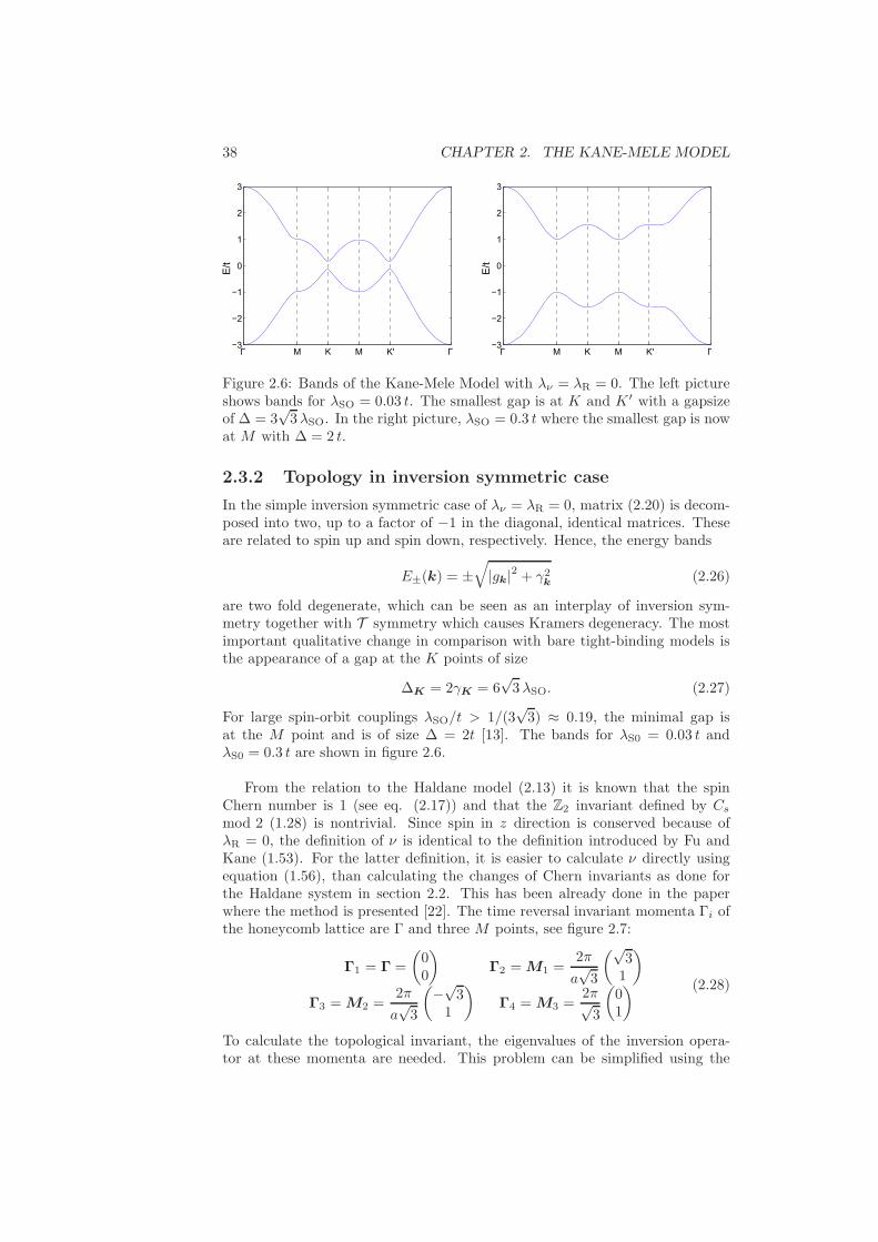
Figure 2.6: Bands of the Kane-Mele Model with λν = λR = 0. The left pictureshows bands for λSO = 0.03 t. The smallest gap is at K and K ′ with a gapsizeof ∆ = 3
√3λSO. In the right picture, λSO = 0.3 t where the smallest gap is now
at M with ∆ = 2 t.
2.3.2 Topology in inversion symmetric case
In the simple inversion symmetric case of λν = λR = 0, matrix (2.20) is decom-posed into two, up to a factor of −1 in the diagonal, identical matrices. Theseare related to spin up and spin down, respectively. Hence, the energy bands
E±(k) = ±√|gk|2 + γ2
k(2.26)
are two fold degenerate, which can be seen as an interplay of inversion sym-metry together with T symmetry which causes Kramers degeneracy. The mostimportant qualitative change in comparison with bare tight-binding models isthe appearance of a gap at the K points of size
∆K = 2γK = 6√3λSO. (2.27)
For large spin-orbit couplings λSO/t > 1/(3√3) ≈ 0.19, the minimal gap is
at the M point and is of size ∆ = 2t [13]. The bands for λS0 = 0.03 t andλS0 = 0.3 t are shown in figure 2.6.
From the relation to the Haldane model (2.13) it is known that the spinChern number is 1 (see eq. (2.17)) and that the Z2 invariant defined by Cs
mod 2 (1.28) is nontrivial. Since spin in z direction is conserved because ofλR = 0, the definition of ν is identical to the definition introduced by Fu andKane (1.53). For the latter definition, it is easier to calculate ν directly usingequation (1.56), than calculating the changes of Chern invariants as done forthe Haldane system in section 2.2. This has been already done in the paperwhere the method is presented [22]. The time reversal invariant momenta Γi ofthe honeycomb lattice are Γ and three M points, see figure 2.7:
Γ1 = Γ =
(00
)Γ2 = M1 =
2π
a√3
(√31
)
Γ3 = M2 =2π
a√3
(−√3
1
)Γ4 = M3 =
2π√3
(01
) (2.28)
To calculate the topological invariant, the eigenvalues of the inversion opera-tor at these momenta are needed. This problem can be simplified using the
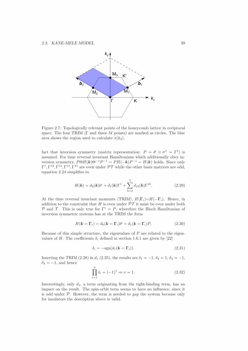
2.3. KANE-MELE MODEL 39
Figure 2.7: Topologically relevant points of the honeycomb lattice in reciprocalspace. The four TRIM (Γ and three M points) are marked as circles. The bluearea shows the region used to calculate x(k2).
fact that inversion symmetry (matrix representation: P = 1 ⊗ σx = Γ1) isassumed. For time reversal invariant Hamiltonians which additionally obey in-version symmetry, PΘH(k)Θ−1P−1 = PH(−k)P−1 = H(k) holds. Since onlyΓ1,Γ12,Γ13,Γ14,Γ15 are even under PT while the other basis matrices are odd,equation 2.24 simplifies to
H(k) = d0(k)1+ d1(k)Γ1 +
5∑
b=2
d1b(k)Γ1b. (2.29)
At the time reversal invariant momenta (TRIM), H(Γi)=H(−Γi). Hence, inaddition to the constraint that H is even under PT it must be even under bothP and T . This is only true for Γ1 = P , wherefore the Bloch Hamiltonian ofinversion symmetric systems has at the TRIM the form
H(k = Γi) = d0(k = Γi)1+ d1(k = Γi)P. (2.30)
Because of this simple structure, the eigenvalues of P are related to the eigen-values of H . The coefficients δi defined in section 1.6.1 are given by [22]
δi = −sgn(d1(k = Γi)). (2.31)
Inserting the TRIM (2.28) in d1 (2.25), the results are δ1 = −1, δ2 = 1, δ3 = −1,δ4 = −1, and hence
4∏
i=1
δi = (−1)1 ⇒ ν = 1. (2.32)
Interestingly, only d1, a term originating from the tight-binding term, has animpact on the result. The spin-orbit term seems to have no influence, since itis odd under P . However, the term is needed to gap the system because onlyfor insulators the description above is valid.
40 CHAPTER 2. THE KANE-MELE MODEL
0 0.5 1 1.5 2−0.5
0
0.5
1
1.5
x
k2/(2π/√
3)0 0.5 1 1.5 2
−0.5
0
0.5
1
1.5
x
k2/(2π/√
3)
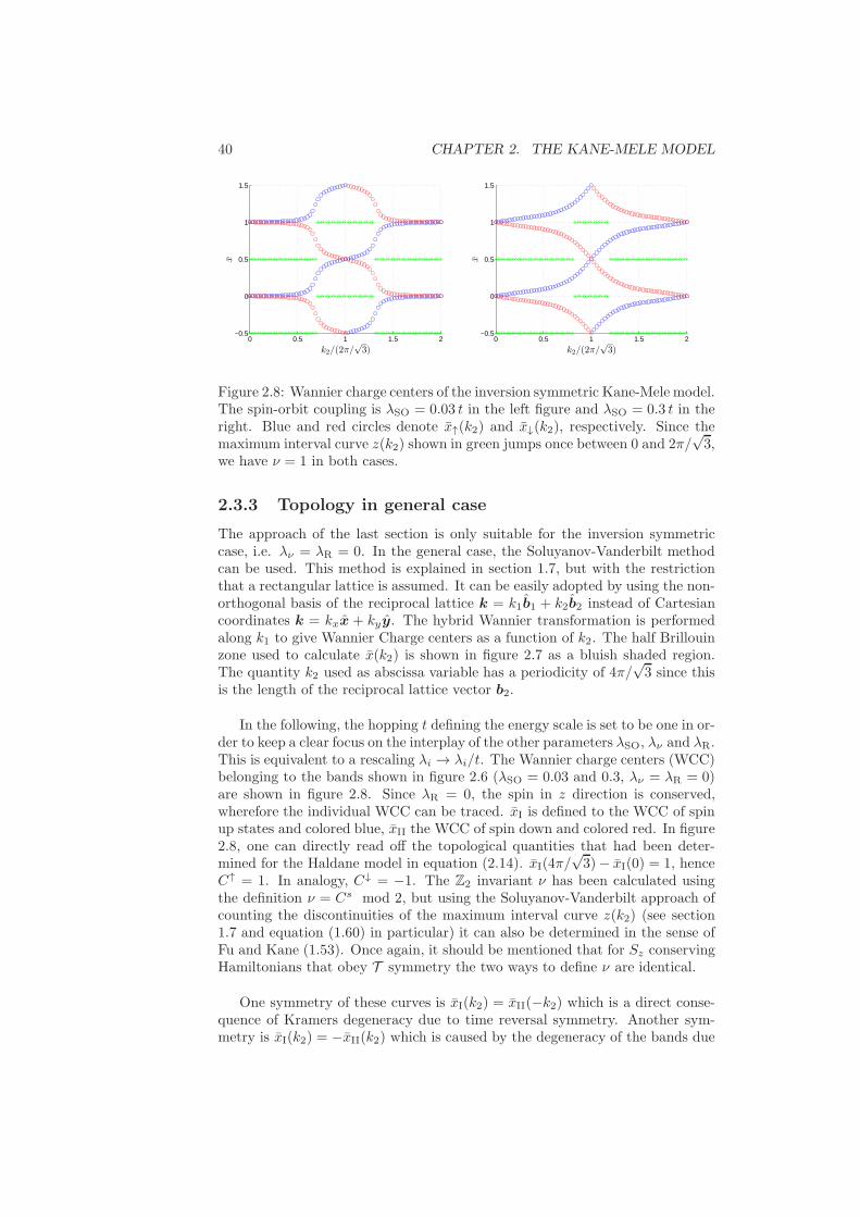
Figure 2.8: Wannier charge centers of the inversion symmetric Kane-Mele model.The spin-orbit coupling is λSO = 0.03 t in the left figure and λSO = 0.3 t in theright. Blue and red circles denote x↑(k2) and x↓(k2), respectively. Since themaximum interval curve z(k2) shown in green jumps once between 0 and 2π/
√3,
we have ν = 1 in both cases.
2.3.3 Topology in general case
The approach of the last section is only suitable for the inversion symmetriccase, i.e. λν = λR = 0. In the general case, the Soluyanov-Vanderbilt methodcan be used. This method is explained in section 1.7, but with the restrictionthat a rectangular lattice is assumed. It can be easily adopted by using the non-orthogonal basis of the reciprocal lattice k = k1b1 + k2b2 instead of Cartesiancoordinates k = kxx + kyy. The hybrid Wannier transformation is performedalong k1 to give Wannier Charge centers as a function of k2. The half Brillouinzone used to calculate x(k2) is shown in figure 2.7 as a bluish shaded region.The quantity k2 used as abscissa variable has a periodicity of 4π/
√3 since this
is the length of the reciprocal lattice vector b2.
In the following, the hopping t defining the energy scale is set to be one in or-der to keep a clear focus on the interplay of the other parameters λSO, λν and λR.This is equivalent to a rescaling λi → λi/t. The Wannier charge centers (WCC)belonging to the bands shown in figure 2.6 (λSO = 0.03 and 0.3, λν = λR = 0)are shown in figure 2.8. Since λR = 0, the spin in z direction is conserved,wherefore the individual WCC can be traced. xI is defined to the WCC of spinup states and colored blue, xII the WCC of spin down and colored red. In figure2.8, one can directly read off the topological quantities that had been deter-mined for the Haldane model in equation (2.14). xI(4π/
√3)− xI(0) = 1, hence
C↑ = 1. In analogy, C↓ = −1. The Z2 invariant ν has been calculated usingthe definition ν = Cs mod 2, but using the Soluyanov-Vanderbilt approach ofcounting the discontinuities of the maximum interval curve z(k2) (see section1.7 and equation (1.60) in particular) it can also be determined in the sense ofFu and Kane (1.53). Once again, it should be mentioned that for Sz conservingHamiltonians that obey T symmetry the two ways to define ν are identical.
One symmetry of these curves is xI(k2) = xII(−k2) which is a direct conse-quence of Kramers degeneracy due to time reversal symmetry. Another sym-metry is xI(k2) = −xII(k2) which is caused by the degeneracy of the bands due

2.3. KANE-MELE MODEL 41
0 0.5 1 1.5 2−0.5
0
0.5
1
1.5
x
k2/(2π/√
3)
Figure 2.9: The left picture shows the bands, the right picture the Wanniercharge center of the Kane-Mele model with λSO = 0.1 t, λν = 0.2 t and λR = 0.
0 0.5 1 1.5 2−0.5
0
0.5
1
1.5
x
k2/(2π/√
3)
Figure 2.10: The left picture shows the bands, the right picture the Wanniercharge center of the Kane-Mele model with λSO = 0.1 t, λν = 0.7 t and λR = 0.
to inversion symmetry. The latter symmetry is broken if an energy differencebetween the sublattices is applied by λν 6= 0. The eigenvalues can be easilycalculated from matrix (2.20):
E↑±(k) = ±
√|gk|2 + (γk + λν)2, (2.33)
E↓±(k) = ±
√|gk|2 + (γk − λν)2. (2.34)
The corresponding bands and the WCC are shown in figure 2.9. The degeneracyof the bands is lifted in most regions of the Brillouin zone, the spin symmetryremains only between Γ and M since γ(kx = 0) = 0 follows from equation(2.22). The system is still a topological insulator, the Chern invariants C↑ = 1and C↓ = −1 are the same as in the case of λν = 0. If λν is increased further,the gap closes at λcν = 3
√3λSO as known from the Haldane model (see section
2.2). If the gap reopens for λν > λcν , the system changes to an trivial bandinsulator. The corresponding bands and WCC are shown in figure 2.10. Notethat the band structures on the left look similar in figure 2.9 and 2.10, althoughthey belong to topologically distinct classes.
If λR 6= 0, the degeneracy of the bands is lifted everywhere except at the
42 CHAPTER 2. THE KANE-MELE MODEL
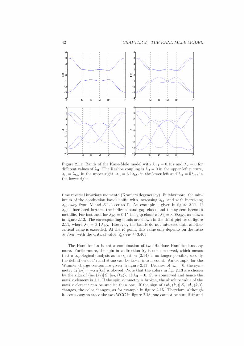
Figure 2.11: Bands of the Kane-Mele model with λSO = 0.15 t and λν = 0 fordifferent values of λR. The Rashba coupling is λR = 0 in the upper left picture,λR = λSO in the upper right, λR = 3.1λSO in the lower left and λR = 5λSO inthe lower right.
time reversal invariant momenta (Kramers degeneracy). Furthermore, the min-imum of the conduction bands shifts with increasing λSO and with increasingλR away from K and K ′ closer to Γ. An example is given in figure 2.11. IfλR is increased further, the indirect band gap closes and the system becomesmetallic. For instance, for λSO = 0.15 the gap closes at λR = 3.09λSO, as shownin figure 2.12. The corresponding bands are shown in the third picture of figure2.11, where λR = 3.1λSO. However, the bands do not intersect until anothercritical value is exceeded. At the K point, this value only depends on the ratioλR/λSO with the critical value λcR/λSO ≈ 3.465.
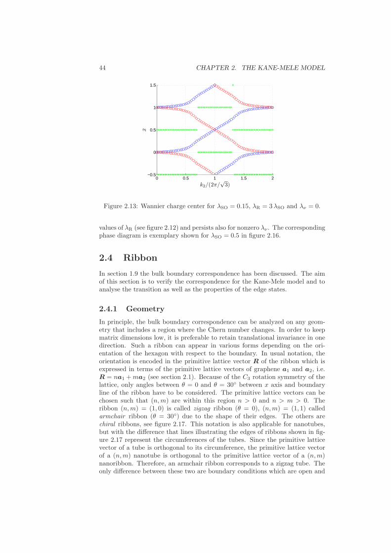
The Hamiltonian is not a combination of two Haldane Hamiltonians anymore. Furthermore, the spin in z direction Sz is not conserved, which meansthat a topological analysis as in equation (2.14) is no longer possible, so onlythe definition of Fu and Kane can be taken into account. An example for theWannier charge centers are given in figure 2.13. Because of λν = 0, the sym-metry xI(k2) = −xII(k2) is obeyed. Note that the colors in fig. 2.13 are chosenby the sign of 〈u2π(k2)|Sz |u2π(k2)〉. If λR = 0, Sz is conserved and hence thematrix element is ±1. If the spin symmetry is broken, the absolute value of thematrix element can be smaller than one. If the sign of
⟨uI2π(k2)
∣∣Sz
∣∣uI2π(k2)⟩
changes, the color changes, as for example in figure 2.15. Therefore, althoughit seems easy to trace the two WCC in figure 2.13, one cannot be sure if xI and
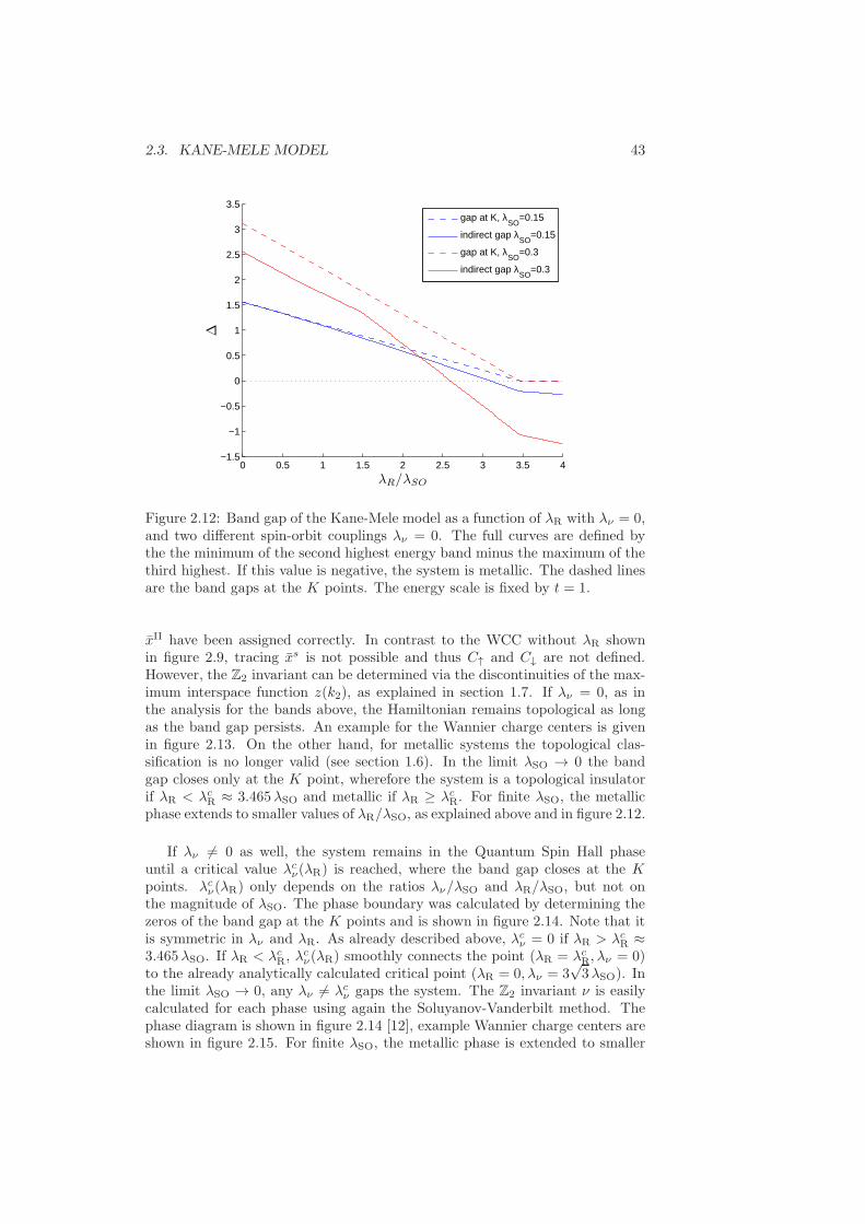
2.3. KANE-MELE MODEL 43
0 0.5 1 1.5 2 2.5 3 3.5 4−1.5
−1
−0.5
0
0.5
1
1.5
2
2.5
3
3.5
λR/λSO
∆
gap at K, λ
SO=0.15
indirect gap λSO
=0.15
gap at K, λSO
=0.3
indirect gap λSO
=0.3
Figure 2.12: Band gap of the Kane-Mele model as a function of λR with λν = 0,and two different spin-orbit couplings λν = 0. The full curves are defined bythe the minimum of the second highest energy band minus the maximum of thethird highest. If this value is negative, the system is metallic. The dashed linesare the band gaps at the K points. The energy scale is fixed by t = 1.
xII have been assigned correctly. In contrast to the WCC without λR shownin figure 2.9, tracing xs is not possible and thus C↑ and C↓ are not defined.However, the Z2 invariant can be determined via the discontinuities of the max-imum interspace function z(k2), as explained in section 1.7. If λν = 0, as inthe analysis for the bands above, the Hamiltonian remains topological as longas the band gap persists. An example for the Wannier charge centers is givenin figure 2.13. On the other hand, for metallic systems the topological clas-sification is no longer valid (see section 1.6). In the limit λSO → 0 the bandgap closes only at the K point, wherefore the system is a topological insulatorif λR < λcR ≈ 3.465λSO and metallic if λR ≥ λcR. For finite λSO, the metallicphase extends to smaller values of λR/λSO, as explained above and in figure 2.12.
If λν 6= 0 as well, the system remains in the Quantum Spin Hall phaseuntil a critical value λcν(λR) is reached, where the band gap closes at the Kpoints. λcν(λR) only depends on the ratios λν/λSO and λR/λSO, but not onthe magnitude of λSO. The phase boundary was calculated by determining thezeros of the band gap at the K points and is shown in figure 2.14. Note that itis symmetric in λν and λR. As already described above, λcν = 0 if λR > λcR ≈3.465λSO. If λR < λcR, λ
cν(λR) smoothly connects the point (λR = λcR, λν = 0)
to the already analytically calculated critical point (λR = 0, λν = 3√3λSO). In
the limit λSO → 0, any λν 6= λcν gaps the system. The Z2 invariant ν is easilycalculated for each phase using again the Soluyanov-Vanderbilt method. Thephase diagram is shown in figure 2.14 [12], example Wannier charge centers areshown in figure 2.15. For finite λSO, the metallic phase is extended to smaller
44 CHAPTER 2. THE KANE-MELE MODEL
0 0.5 1 1.5 2−0.5
0
0.5
1
1.5
x
k2/(2π/√
3)
Figure 2.13: Wannier charge center for λSO = 0.15, λR = 3λSO and λν = 0.
values of λR (see figure 2.12) and persists also for nonzero λν . The correspondingphase diagram is exemplary shown for λSO = 0.5 in figure 2.16.
2.4 Ribbon
In section 1.9 the bulk boundary correspondence has been discussed. The aimof this section is to verify the correspondence for the Kane-Mele model and toanalyse the transition as well as the properties of the edge states.
2.4.1 Geometry
In principle, the bulk boundary correspondence can be analyzed on any geom-etry that includes a region where the Chern number changes. In order to keepmatrix dimensions low, it is preferable to retain translational invariance in onedirection. Such a ribbon can appear in various forms depending on the ori-entation of the hexagon with respect to the boundary. In usual notation, theorientation is encoded in the primitive lattice vector R of the ribbon which isexpressed in terms of the primitive lattice vectors of graphene a1 and a2, i.e.R = na1 +ma2 (see section 2.1). Because of the C3 rotation symmetry of thelattice, only angles between θ = 0 and θ = 30 between x axis and boundaryline of the ribbon have to be considered. The primitive lattice vectors can bechosen such that (n,m) are within this region n > 0 and n > m > 0. Theribbon (n,m) = (1, 0) is called zigzag ribbon (θ = 0), (n,m) = (1, 1) calledarmchair ribbon (θ = 30) due to the shape of their edges. The others arechiral ribbons, see figure 2.17. This notation is also applicable for nanotubes,but with the difference that lines illustrating the edges of ribbons shown in fig-ure 2.17 represent the circumferences of the tubes. Since the primitive latticevector of a tube is orthogonal to its circumference, the primitive lattice vectorof a (n,m) nanotube is orthogonal to the primitive lattice vector of a (n,m)nanoribbon. Therefore, an armchair ribbon corresponds to a zigzag tube. Theonly difference between these two are boundary conditions which are open and
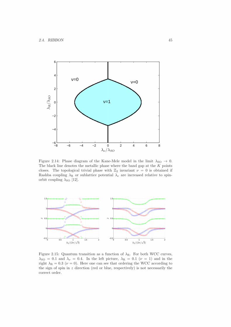
2.4. RIBBON 45
−8 −6 −4 −2 0 2 4 6 8−6
−4
−2
0
2
4
6
λν/λSO
λR/λ
SO
ν=1
ν=0 ν=0
Figure 2.14: Phase diagram of the Kane-Mele model in the limit λSO → 0.The black line denotes the metallic phase where the band gap at the K pointscloses. The topological trivial phase with Z2 invariant ν = 0 is obtained ifRashba coupling λR or sublattice potential λν are increased relative to spin-orbit coupling λSO [12].
0 0.5 1 1.5 2−0.5
0
0.5
1
1.5
x
k2/(2π/√
3)0 0.5 1 1.5 2
−0.5
0
0.5
1
1.5
x
k2/(2π/√
3)
Figure 2.15: Quantum transition as a function of λR. For both WCC curves,λSO = 0.1 and λν = 0.4. In the left picture, λR = 0.1 (ν = 1) and in theright λR = 0.3 (ν = 0). Here one can see that ordering the WCC according tothe sign of spin in z direction (red or blue, respectively) is not necessarily thecorrect order.
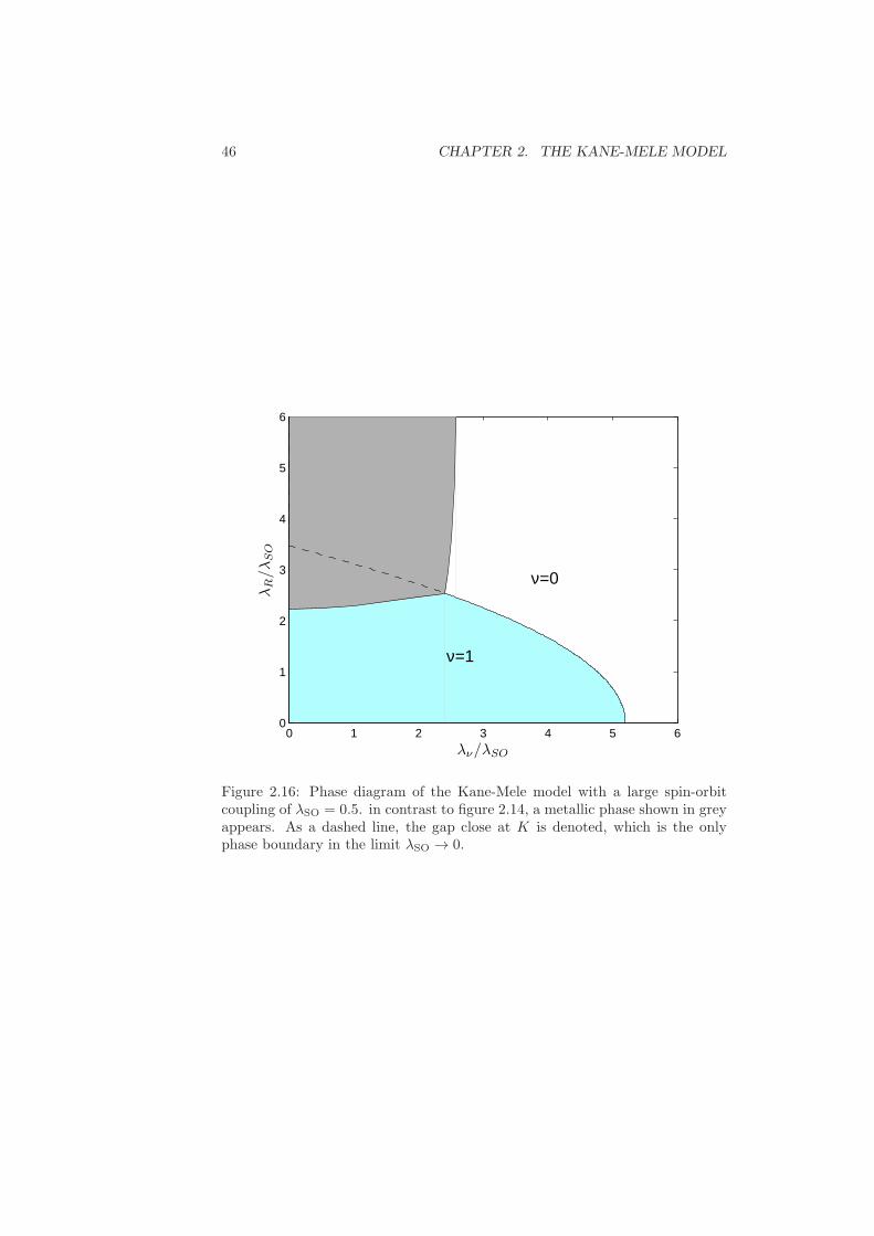
46 CHAPTER 2. THE KANE-MELE MODEL
0 1 2 3 4 5 60
1
2
3
4
5
6
λν/λSO
λR/λ
SO
ν=1
ν=0
Figure 2.16: Phase diagram of the Kane-Mele model with a large spin-orbitcoupling of λSO = 0.5. in contrast to figure 2.14, a metallic phase shown in greyappears. As a dashed line, the gap close at K is denoted, which is the onlyphase boundary in the limit λSO → 0.
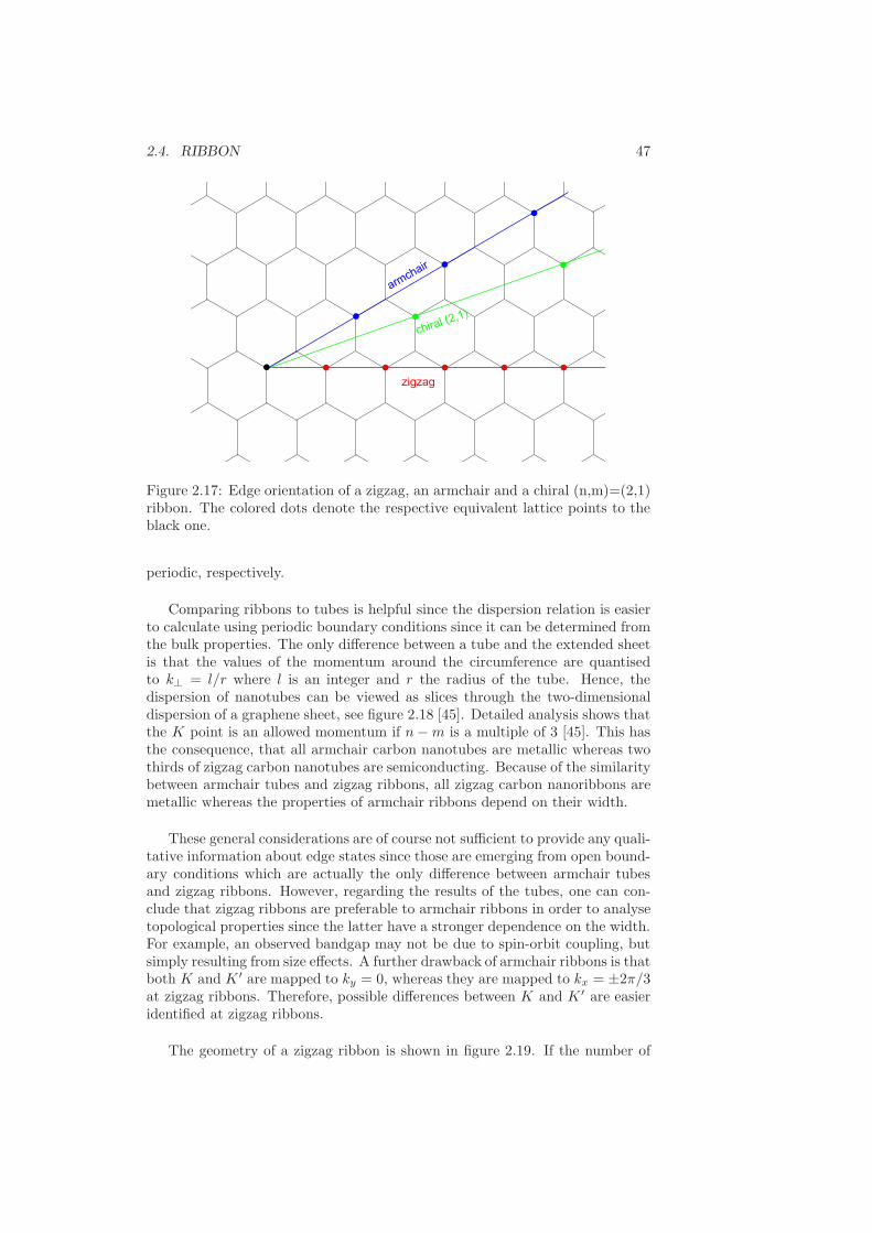
2.4. RIBBON 47
Figure 2.17: Edge orientation of a zigzag, an armchair and a chiral (n,m)=(2,1)ribbon. The colored dots denote the respective equivalent lattice points to theblack one.
periodic, respectively.
Comparing ribbons to tubes is helpful since the dispersion relation is easierto calculate using periodic boundary conditions since it can be determined fromthe bulk properties. The only difference between a tube and the extended sheetis that the values of the momentum around the circumference are quantisedto k⊥ = l/r where l is an integer and r the radius of the tube. Hence, thedispersion of nanotubes can be viewed as slices through the two-dimensionaldispersion of a graphene sheet, see figure 2.18 [45]. Detailed analysis shows thatthe K point is an allowed momentum if n−m is a multiple of 3 [45]. This hasthe consequence, that all armchair carbon nanotubes are metallic whereas twothirds of zigzag carbon nanotubes are semiconducting. Because of the similaritybetween armchair tubes and zigzag ribbons, all zigzag carbon nanoribbons aremetallic whereas the properties of armchair ribbons depend on their width.
These general considerations are of course not sufficient to provide any quali-tative information about edge states since those are emerging from open bound-ary conditions which are actually the only difference between armchair tubesand zigzag ribbons. However, regarding the results of the tubes, one can con-clude that zigzag ribbons are preferable to armchair ribbons in order to analysetopological properties since the latter have a stronger dependence on the width.For example, an observed bandgap may not be due to spin-orbit coupling, butsimply resulting from size effects. A further drawback of armchair ribbons is thatboth K and K ′ are mapped to ky = 0, whereas they are mapped to kx = ±2π/3at zigzag ribbons. Therefore, possible differences between K and K ′ are easieridentified at zigzag ribbons.
The geometry of a zigzag ribbon is shown in figure 2.19. If the number of
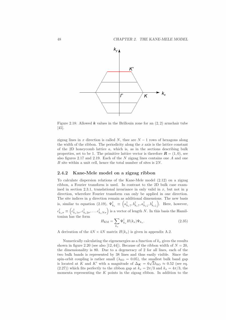
48 CHAPTER 2. THE KANE-MELE MODEL
Figure 2.18: Allowed k values in the Brillouin zone for an (2, 2) armchair tube[45].
zigzag lines in x direction is called N , thee are N − 1 rows of hexagons alongthe width of the ribbon. The periodicity along the x axis is the lattice constantof the 2D honeycomb lattice a, which is, as in the sections describing bulkproperties, set to be 1. The primitive lattice vector is therefore R = (1, 0), seealso figures 2.17 and 2.19. Each of the N zigzag lines contains one A and oneB site within a unit cell, hence the total number of sites is 2N .
2.4.2 Kane-Mele model on a zigzag ribbon
To calculate dispersion relations of the Kane-Mele model (2.12) on a zigzagribbon, a Fourier transform is used. In contrast to the 2D bulk case exam-ined in section 2.3.1, translational invariance in only valid in x, but not in ydirection, wherefore Fourier transform can only be applied in one direction.The site indices in y direction remain as additional dimensions. The new basis
is, similar to equation (2.19), Ψ†kx
≡(a†kx↑, b
†kx↑, a
†kx↓, b
†kx↓
). Here, however,
c†kxσ≡(c†kx1σ
, c†kx2σ, . . . c†kxNσ
)is a vector of length N . In this basis the Hamil-
tonian has the formHKM =
∑
kx
Ψ†kxH(kx)Ψkx
. (2.35)
A derivation of the 4N × 4N matrix H(kx) is given in appendix A.2.
Numerically calculating the eigenenergies as a function of kx gives the resultsshown in figure 2.20 (see also [12,44]). Because of the ribbon width of N = 20,the dimensionality is 80. Due to a degeneracy of 2 for all lines, each of thetwo bulk bands is represented by 38 lines and thus easily visible. Since thespin-orbit coupling is rather small (λSO = 0.05), the smallest bulk band gapis located at K and K ′ with a magnitude of ∆K = 6
√3λSO ≈ 0.52 (see eq.
(2.27)) which fits perfectly to the ribbon gap at kx = 2π/3 and kx = 4π/3, themomenta representing the K points in the zigzag ribbon. In addition to the
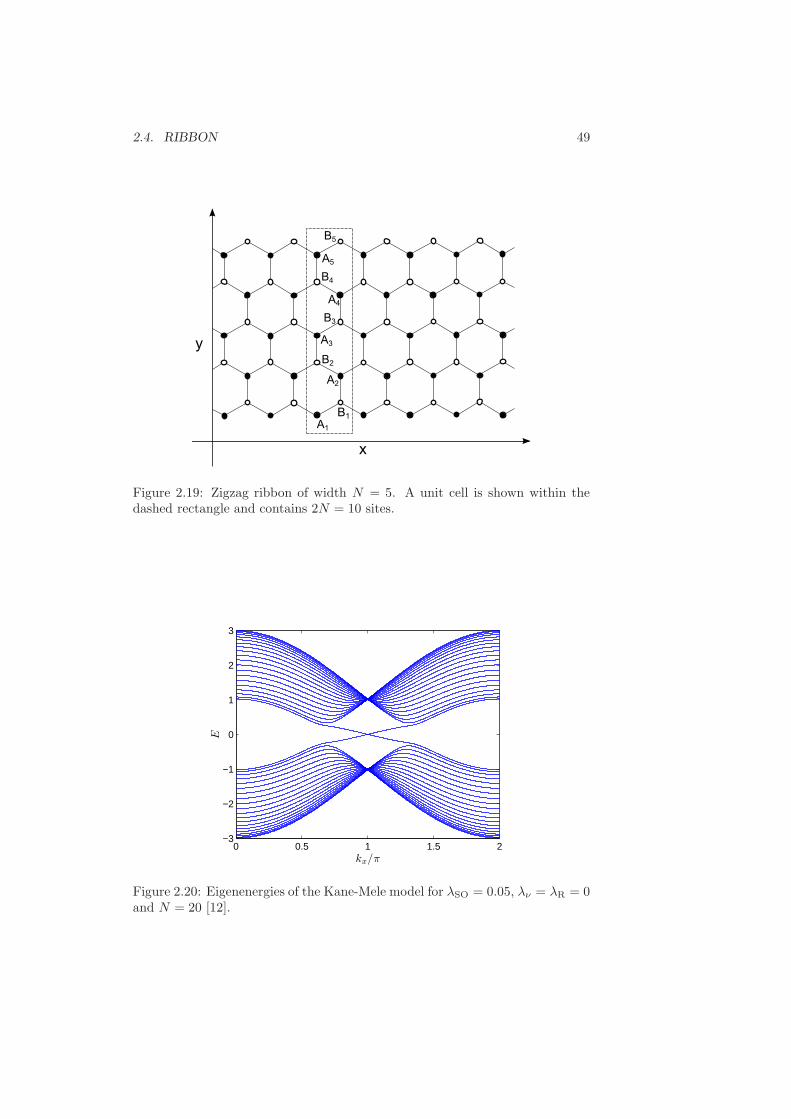
2.4. RIBBON 49
Figure 2.19: Zigzag ribbon of width N = 5. A unit cell is shown within thedashed rectangle and contains 2N = 10 sites.
0 0.5 1 1.5 2−3
−2
−1
0
1
2
3
kx/π
E
Figure 2.20: Eigenenergies of the Kane-Mele model for λSO = 0.05, λν = λR = 0and N = 20 [12].
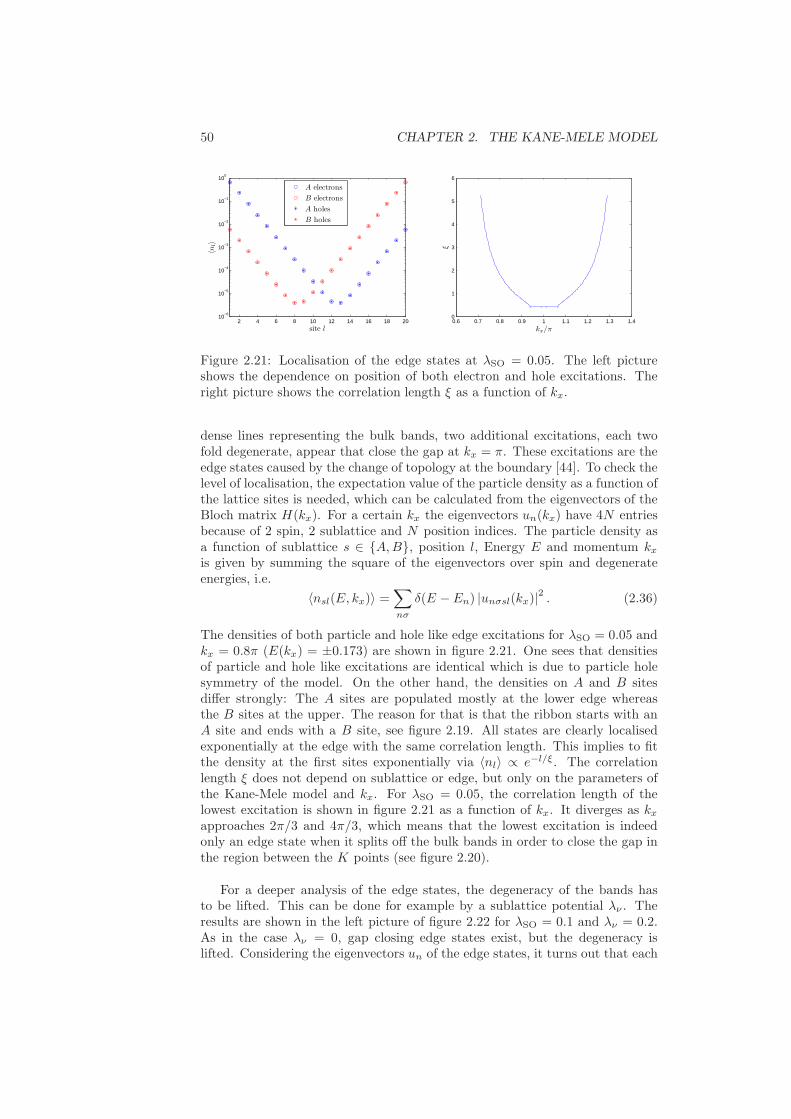
50 CHAPTER 2. THE KANE-MELE MODEL
2 4 6 8 10 12 14 16 18 2010
−6
10−5
10−4
10−3
10−2
10−1
100
site l
〈nl〉
A electrons
B electrons
A holes
B holes
0.6 0.7 0.8 0.9 1 1.1 1.2 1.3 1.40
1
2
3
4
5
6
kx/π
ξ
Figure 2.21: Localisation of the edge states at λSO = 0.05. The left pictureshows the dependence on position of both electron and hole excitations. Theright picture shows the correlation length ξ as a function of kx.
dense lines representing the bulk bands, two additional excitations, each twofold degenerate, appear that close the gap at kx = π. These excitations are theedge states caused by the change of topology at the boundary [44]. To check thelevel of localisation, the expectation value of the particle density as a function ofthe lattice sites is needed, which can be calculated from the eigenvectors of theBloch matrix H(kx). For a certain kx the eigenvectors un(kx) have 4N entriesbecause of 2 spin, 2 sublattice and N position indices. The particle density asa function of sublattice s ∈ A,B, position l, Energy E and momentum kxis given by summing the square of the eigenvectors over spin and degenerateenergies, i.e.
〈nsl(E, kx)〉 =∑
nσ
δ(E − En) |unσsl(kx)|2 . (2.36)
The densities of both particle and hole like edge excitations for λSO = 0.05 andkx = 0.8π (E(kx) = ±0.173) are shown in figure 2.21. One sees that densitiesof particle and hole like excitations are identical which is due to particle holesymmetry of the model. On the other hand, the densities on A and B sitesdiffer strongly: The A sites are populated mostly at the lower edge whereasthe B sites at the upper. The reason for that is that the ribbon starts with anA site and ends with a B site, see figure 2.19. All states are clearly localisedexponentially at the edge with the same correlation length. This implies to fitthe density at the first sites exponentially via 〈nl〉 ∝ e−l/ξ. The correlationlength ξ does not depend on sublattice or edge, but only on the parameters ofthe Kane-Mele model and kx. For λSO = 0.05, the correlation length of thelowest excitation is shown in figure 2.21 as a function of kx. It diverges as kxapproaches 2π/3 and 4π/3, which means that the lowest excitation is indeedonly an edge state when it splits off the bulk bands in order to close the gap inthe region between the K points (see figure 2.20).
For a deeper analysis of the edge states, the degeneracy of the bands hasto be lifted. This can be done for example by a sublattice potential λν . Theresults are shown in the left picture of figure 2.22 for λSO = 0.1 and λν = 0.2.As in the case λν = 0, gap closing edge states exist, but the degeneracy islifted. Considering the eigenvectors un of the edge states, it turns out that each
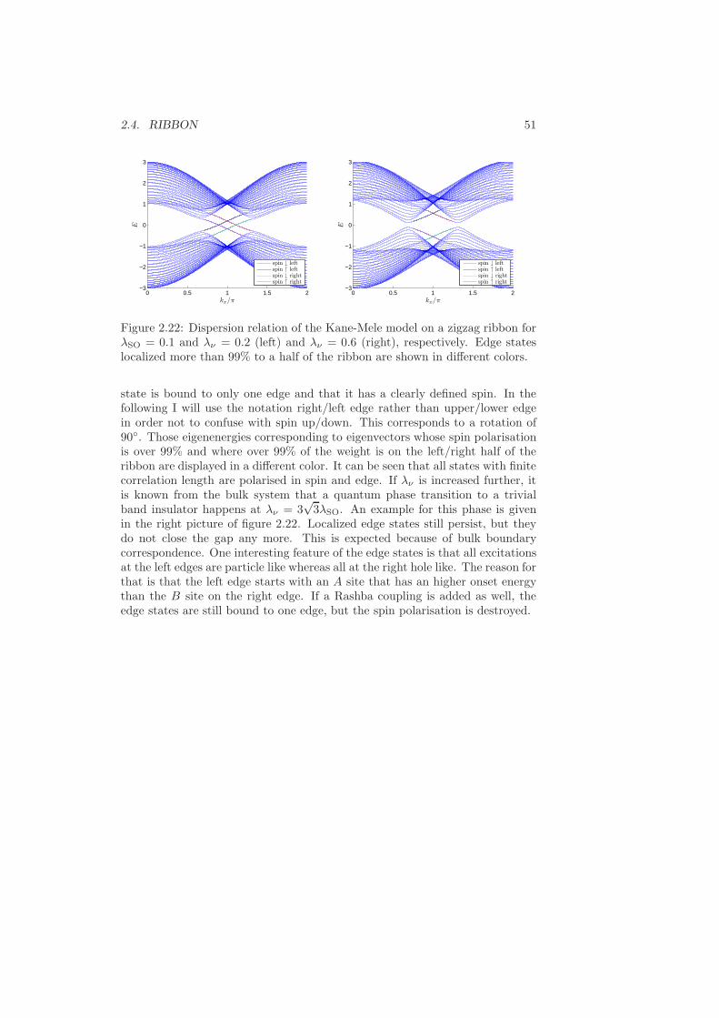
2.4. RIBBON 51
0 0.5 1 1.5 2−3
−2
−1
0
1
2
3
kx/π
E
spin ↓ leftspin ↑ leftspin ↓ rightspin ↑ right
0 0.5 1 1.5 2−3
−2
−1
0
1
2
3
kx/π
E
spin ↓ leftspin ↑ leftspin ↓ rightspin ↑ right
Figure 2.22: Dispersion relation of the Kane-Mele model on a zigzag ribbon forλSO = 0.1 and λν = 0.2 (left) and λν = 0.6 (right), respectively. Edge stateslocalized more than 99% to a half of the ribbon are shown in different colors.
state is bound to only one edge and that it has a clearly defined spin. In thefollowing I will use the notation right/left edge rather than upper/lower edgein order not to confuse with spin up/down. This corresponds to a rotation of90. Those eigenenergies corresponding to eigenvectors whose spin polarisationis over 99% and where over 99% of the weight is on the left/right half of theribbon are displayed in a different color. It can be seen that all states with finitecorrelation length are polarised in spin and edge. If λν is increased further, itis known from the bulk system that a quantum phase transition to a trivialband insulator happens at λν = 3
√3λSO. An example for this phase is given
in the right picture of figure 2.22. Localized edge states still persist, but theydo not close the gap any more. This is expected because of bulk boundarycorrespondence. One interesting feature of the edge states is that all excitationsat the left edges are particle like whereas all at the right hole like. The reason forthat is that the left edge starts with an A site that has an higher onset energythan the B site on the right edge. If a Rashba coupling is added as well, theedge states are still bound to one edge, but the spin polarisation is destroyed.

52 CHAPTER 2. THE KANE-MELE MODEL
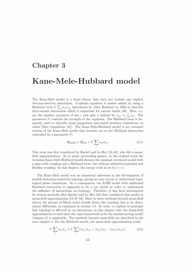
Chapter 3
Kane-Mele-Hubbard model
The Kane-Mele model is a band theory that does not include any explicitelectron-electron interaction. Coulomb repulsion is easiest added by using aHubbard term U
∑i ni↑ni↓ introduced by John Hubbard in 1963 to describe
intra-atomic interaction which is important for narrow bands [46]. Here, niσ
are the number operators of site i and spin σ defined by niσ ≡ c†iσciσ. Theparameter U controls the strength of the repulsion. The Hubbard term is fre-quently used to describe band magnetism and metal insulator transitions, socalled Mott transitions [47]. The Kane-Mele-Hubbard model is an extendedversion of the Kane-Mele model that includes an on site Hubbard interactioncontrolled by a parameter U ,
HKMH ≡ HKM + U∑
i
ni↑ni↓. (3.1)
This term was first considered by Rachel and Le Hur [13, 48], who did a mean-field approximation. As in many proceeding papers, in the original work theterminus Kane-Mele-Hubbard model denotes the minimal correlated model witha spin-orbit coupling and a Hubbard term, but without sublattice potential andRashba coupling. In this chapter, the energy scale is set by t = 1.
The Kane-Mele model was an important milestone in the development ofmodels featuring nontrivial topology giving an easy access to understand topo-logical phase transitions. As a consequence, the KMH model with additionalHubbard interaction is supposed to be a toy model in order to understandthe influence of interactions on topology. Therefore, it has been investigatedby several methods after Rachel and Le Hur [48] first considered this model inmean-field approximation [13,49–52]. Since in these methods beyond mean-fieldtheory the picture of Bloch states breaks down, the topology has to be deter-mined differently, as explained in section 1.8. In order to explain in principlehow topology is affected by an interaction, in this chapter only the mean-fieldapproximation is used since the same framework as for the noninteracting model(chapter 2) is applicable. The methods beyond mean-field are described in thenext chapter 4. For the Hubbard model, the mean-field approximation reads:
U∑
i
ni↑ni↓ ≈ U∑
i
(〈ni↑〉ni↓ + 〈ni↓〉ni↑ − 〈ni↑〉〈ni↓〉). (3.2)
53
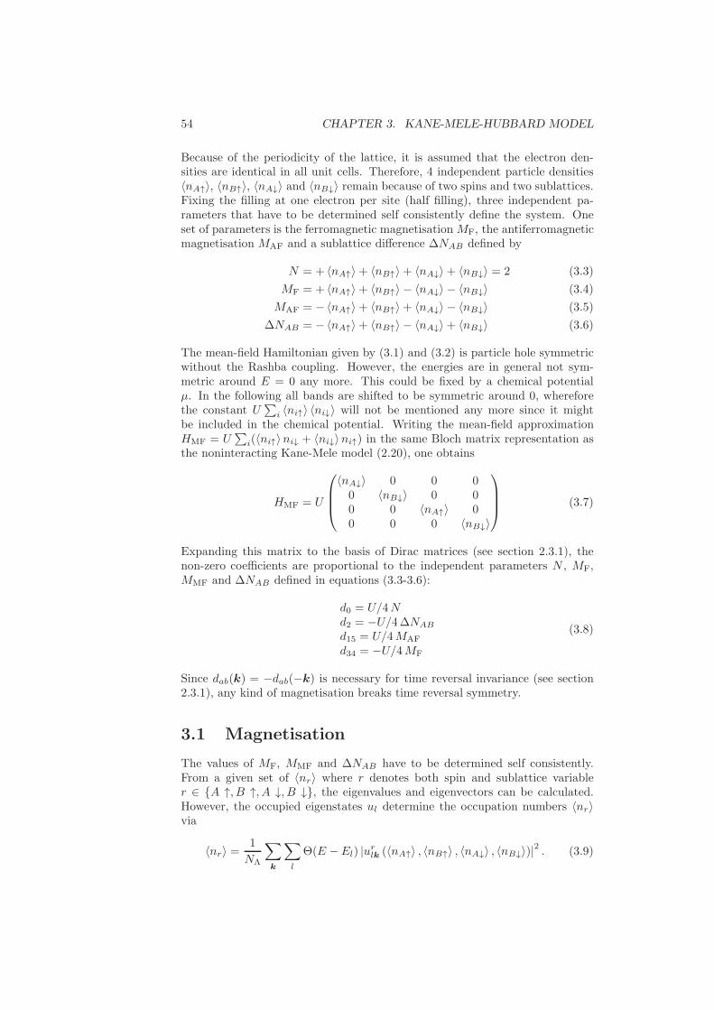
54 CHAPTER 3. KANE-MELE-HUBBARD MODEL
Because of the periodicity of the lattice, it is assumed that the electron den-sities are identical in all unit cells. Therefore, 4 independent particle densities〈nA↑〉, 〈nB↑〉, 〈nA↓〉 and 〈nB↓〉 remain because of two spins and two sublattices.Fixing the filling at one electron per site (half filling), three independent pa-rameters that have to be determined self consistently define the system. Oneset of parameters is the ferromagnetic magnetisationMF, the antiferromagneticmagnetisation MAF and a sublattice difference ∆NAB defined by
N = + 〈nA↑〉+ 〈nB↑〉+ 〈nA↓〉+ 〈nB↓〉 = 2 (3.3)
MF = + 〈nA↑〉+ 〈nB↑〉 − 〈nA↓〉 − 〈nB↓〉 (3.4)
MAF = −〈nA↑〉+ 〈nB↑〉+ 〈nA↓〉 − 〈nB↓〉 (3.5)
∆NAB = −〈nA↑〉+ 〈nB↑〉 − 〈nA↓〉+ 〈nB↓〉 (3.6)
The mean-field Hamiltonian given by (3.1) and (3.2) is particle hole symmetricwithout the Rashba coupling. However, the energies are in general not sym-metric around E = 0 any more. This could be fixed by a chemical potentialµ. In the following all bands are shifted to be symmetric around 0, whereforethe constant U
∑i 〈ni↑〉 〈ni↓〉 will not be mentioned any more since it might
be included in the chemical potential. Writing the mean-field approximationHMF = U
∑i(〈ni↑〉ni↓ + 〈ni↓〉ni↑) in the same Bloch matrix representation as
the noninteracting Kane-Mele model (2.20), one obtains
HMF = U
〈nA↓〉 0 0 00 〈nB↓〉 0 00 0 〈nA↑〉 00 0 0 〈nB↓〉
(3.7)
Expanding this matrix to the basis of Dirac matrices (see section 2.3.1), thenon-zero coefficients are proportional to the independent parameters N , MF,MMF and ∆NAB defined in equations (3.3-3.6):
d0 = U/4Nd2 = −U/4∆NAB
d15 = U/4MAF
d34 = −U/4MF
(3.8)
Since dab(k) = −dab(−k) is necessary for time reversal invariance (see section2.3.1), any kind of magnetisation breaks time reversal symmetry.
3.1 Magnetisation
The values of MF, MMF and ∆NAB have to be determined self consistently.From a given set of 〈nr〉 where r denotes both spin and sublattice variabler ∈ A ↑, B ↑, A ↓, B ↓, the eigenvalues and eigenvectors can be calculated.However, the occupied eigenstates ul determine the occupation numbers 〈nr〉via
〈nr〉 =1
NΛ
∑
k
∑
l
Θ(E − El) |urlk (〈nA↑〉 , 〈nB↑〉 , 〈nA↓〉 , 〈nB↓〉)|2 . (3.9)
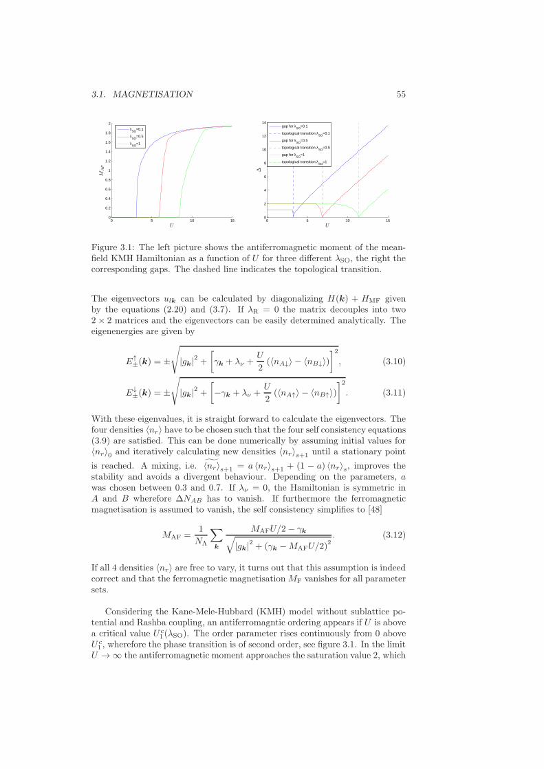
3.1. MAGNETISATION 55
0 5 10 150
0.2
0.4
0.6
0.8
1
1.2
1.4
1.6
1.8
2
U
MA
F
λSO
=0.1
λSO
=0.5
λSO
=1
0 5 10 150
2
4
6
8
10
12
14
U
∆
gap for λ
SO=0.1
topological transition λSO
=0.1
gap for λSO
=0.5
topological transition λSO
=0.5
gap for λSO
=1
topological transition λSO
=1
Figure 3.1: The left picture shows the antiferromagnetic moment of the mean-field KMH Hamiltonian as a function of U for three different λSO, the right thecorresponding gaps. The dashed line indicates the topological transition.
The eigenvectors ulk can be calculated by diagonalizing H(k) + HMF givenby the equations (2.20) and (3.7). If λR = 0 the matrix decouples into two2 × 2 matrices and the eigenvectors can be easily determined analytically. Theeigenenergies are given by
E↑±(k) = ±
√
|gk|2 +[γk + λν +
U
2(〈nA↓〉 − 〈nB↓〉)
]2, (3.10)
E↓±(k) = ±
√
|gk|2 +[−γk + λν +
U
2(〈nA↑〉 − 〈nB↑〉)
]2. (3.11)
With these eigenvalues, it is straight forward to calculate the eigenvectors. Thefour densities 〈nr〉 have to be chosen such that the four self consistency equations(3.9) are satisfied. This can be done numerically by assuming initial values for〈nr〉0 and iteratively calculating new densities 〈nr〉s+1 until a stationary point
is reached. A mixing, i.e. 〈nr〉s+1 = a 〈nr〉s+1 + (1 − a) 〈nr〉s, improves thestability and avoids a divergent behaviour. Depending on the parameters, awas chosen between 0.3 and 0.7. If λν = 0, the Hamiltonian is symmetric inA and B wherefore ∆NAB has to vanish. If furthermore the ferromagneticmagnetisation is assumed to vanish, the self consistency simplifies to [48]
MAF =1
NΛ
∑
k
MAFU/2− γk√|gk|2 + (γk −MAFU/2)
2. (3.12)
If all 4 densities 〈nr〉 are free to vary, it turns out that this assumption is indeedcorrect and that the ferromagnetic magnetisationMF vanishes for all parametersets.
Considering the Kane-Mele-Hubbard (KMH) model without sublattice po-tential and Rashba coupling, an antiferromagntic ordering appears if U is abovea critical value U c
1 (λSO). The order parameter rises continuously from 0 aboveU c1 , wherefore the phase transition is of second order, see figure 3.1. In the limit
U → ∞ the antiferromagnetic moment approaches the saturation value 2, which
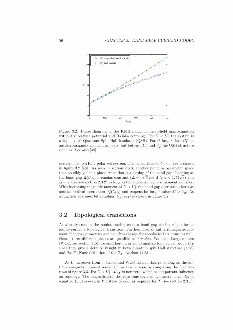
56 CHAPTER 3. KANE-MELE-HUBBARD MODEL
0 0.2 0.4 0.6 0.8 10
2
4
6
8
10
12
λSO
U
Uc1: magnetisation threshold
Uc2: gap closing
Figure 3.2: Phase diagram of the KMH model in mean-field approximationwithout sublattice potential and Rashba coupling. For U < U c
1 the system isa topological Quantum Spin Hall insulator (QSH). For U larger than U c
1 anantiferromagnetic moment appears, but between U c
1 and U c2 the QSH structure
remains. See also [48].
corresponds to a fully polarized system. The dependence of U c1 on λSO is shown
in figure 3.2 [48]. As seen in section 2.3.3, another point in parameter spacethat possibly yields a phase transition is a closing of the band gap. Looking atthe band gap ∆(U), it remains constant (∆ = 6
√3λSO if λSO < 1/(3
√3) and
∆ = 2 else, see section 2.3.2) as long as the antiferromagnetic moment vanishes.With increasing magnetic moment at U > U c
1 the band gap decreases, closes atanother critical interaction U c
2(λSO) and reopens for larger values U > U c2 . As
a function of spin-orbit coupling, U c2(λSO) is shown in figure 3.2.
3.2 Topological transitions
As already seen in the noninteracting case, a band gap closing might be anindication for a topological transition. Furthermore, an antiferromagnetic mo-ment changes symmetries and can thus change the topological structure as well.Hence, three different phases are possible as U varies. Wannier charge centers(WCC, see section 1.5) are used here in order to analyse topological propertiessince they give a detailed insight in both quantum spin Hall structure (1.28)and the Fu-Kane definition of the Z2 invariant (1.53).
As U increases from 0, bands and WCC do not change as long as the an-tiferromagnetic moment remains 0, as can be seen by comparing the first tworows of figure 3.3. For U > U c
1 , MAF is non zero, which has important influenceon topology. The magnetisation destroys time reversal symmetry, since d15 inequation (3.8) is even in k instead of odd, as required for T (see section 2.3.1).
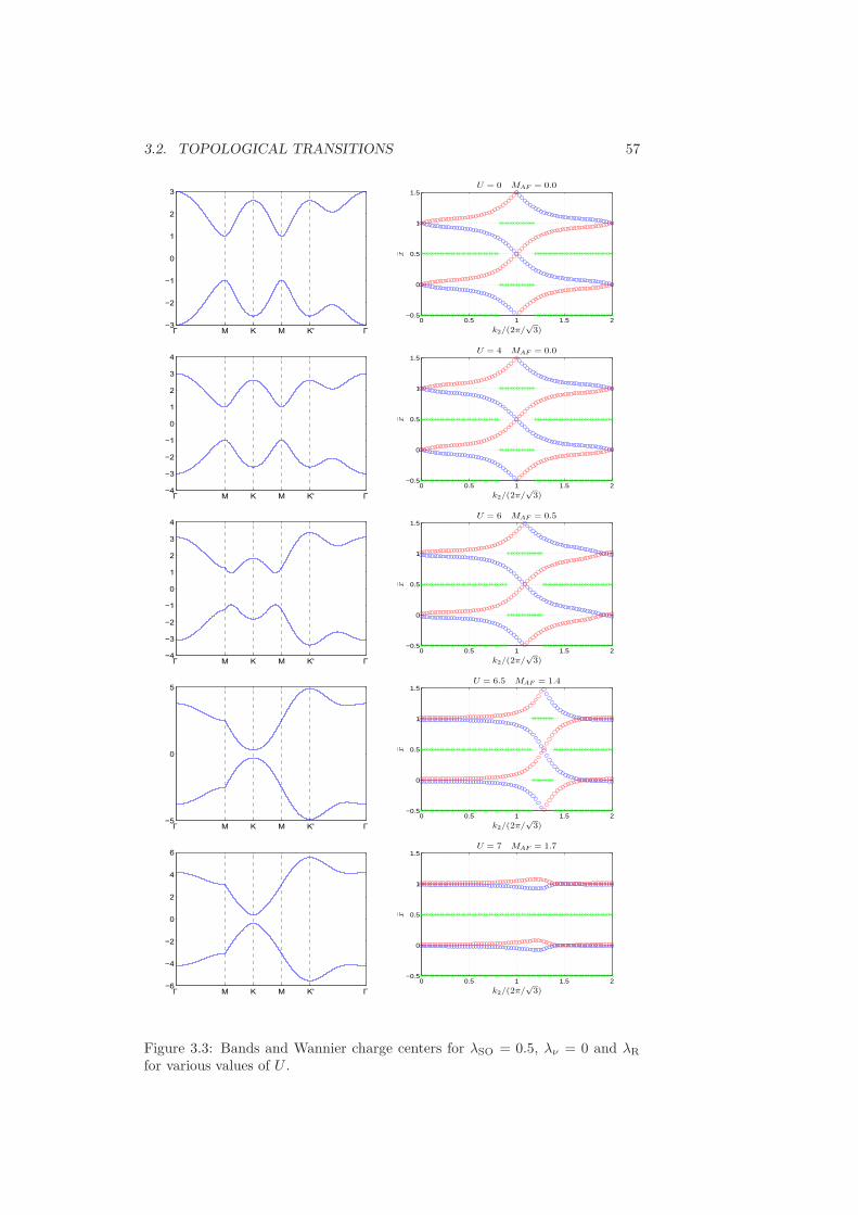
3.2. TOPOLOGICAL TRANSITIONS 57
0 0.5 1 1.5 2−0.5
0
0.5
1
1.5
x
k2/(2π/√
3)
U = 0 MAF = 0.0
0 0.5 1 1.5 2−0.5
0
0.5
1
1.5
x
k2/(2π/√
3)
U = 4 MAF = 0.0
0 0.5 1 1.5 2−0.5
0
0.5
1
1.5
x
k2/(2π/√
3)
U = 6 MAF = 0.5
0 0.5 1 1.5 2−0.5
0
0.5
1
1.5
x
k2/(2π/√
3)
U = 6.5 MAF = 1.4
0 0.5 1 1.5 2−0.5
0
0.5
1
1.5
x
k2/(2π/√
3)
U = 7 MAF = 1.7
Figure 3.3: Bands and Wannier charge centers for λSO = 0.5, λν = 0 and λRfor various values of U .
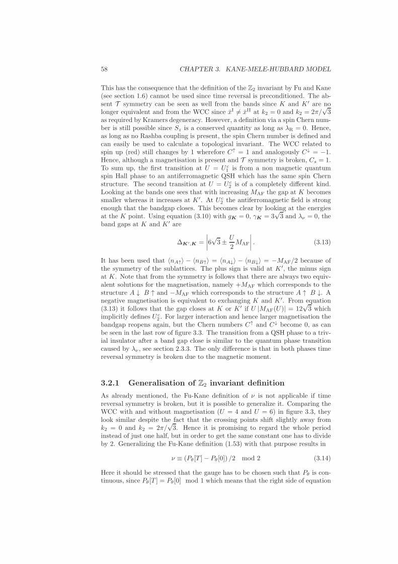
58 CHAPTER 3. KANE-MELE-HUBBARD MODEL
This has the consequence that the definition of the Z2 invariant by Fu and Kane(see section 1.6) cannot be used since time reversal is preconditioned. The ab-sent T symmetry can be seen as well from the bands since K and K ′ are nolonger equivalent and from the WCC since xI 6= xII at k2 = 0 and k2 = 2π/
√3
as required by Kramers degeneracy. However, a definition via a spin Chern num-ber is still possible since Sz is a conserved quantity as long as λR = 0. Hence,as long as no Rashba coupling is present, the spin Chern number is defined andcan easily be used to calculate a topological invariant. The WCC related tospin up (red) still changes by 1 wherefore C↑ = 1 and analogously C↓ = −1.Hence, although a magnetisation is present and T symmetry is broken, Cs = 1.To sum up, the first transition at U = U c
1 is from a non magnetic quantumspin Hall phase to an antiferromagnetic QSH which has the same spin Chernstructure. The second transition at U = U c
2 is of a completely different kind.Looking at the bands one sees that with increasing MAF the gap at K becomessmaller whereas it increases at K ′. At U c
2 the antiferromagnetic field is strongenough that the bandgap closes. This becomes clear by looking at the energiesat the K point. Using equation (3.10) with gK = 0, γK = 3
√3 and λν = 0, the
band gaps at K and K ′ are
∆K′,K =
∣∣∣∣6√3± U
2MAF
∣∣∣∣ . (3.13)
It has been used that 〈nA↑〉 − 〈nB↑〉 = 〈nA↓〉 − 〈nB↓〉 = −MAF/2 because ofthe symmetry of the sublattices. The plus sign is valid at K ′, the minus signat K. Note that from the symmetry is follows that there are always two equiv-alent solutions for the magnetisation, namely +MAF which corresponds to thestructure A ↓ B ↑ and −MAF which corresponds to the structure A ↑ B ↓. Anegative magnetisation is equivalent to exchanging K and K ′. From equation(3.13) it follows that the gap closes at K or K ′ if U |MAF(U)| = 12
√3 which
implicitly defines U c2 . For larger interaction and hence larger magnetisation the
bandgap reopens again, but the Chern numbers C↑ and C↓ become 0, as canbe seen in the last row of figure 3.3. The transition from a QSH phase to a triv-ial insulator after a band gap close is similar to the quantum phase transitioncaused by λν , see section 2.3.3. The only difference is that in both phases timereversal symmetry is broken due to the magnetic moment.
3.2.1 Generalisation of Z2 invariant definition
As already mentioned, the Fu-Kane definition of ν is not applicable if timereversal symmetry is broken, but it is possible to generalize it. Comparing theWCC with and without magnetisation (U = 4 and U = 6) in figure 3.3, theylook similar despite the fact that the crossing points shift slightly away fromk2 = 0 and k2 = 2π/
√3. Hence it is promising to regard the whole period
instead of just one half, but in order to get the same constant one has to divideby 2. Generalizing the Fu-Kane definition (1.53) with that purpose results in
ν ≡ (Pθ[T ]− Pθ[0]) /2 mod 2 (3.14)
Here it should be stressed that the gauge has to be chosen such that Pθ is con-tinuous, since Pθ[T ] = Pθ[0] mod 1 which means that the right side of equation
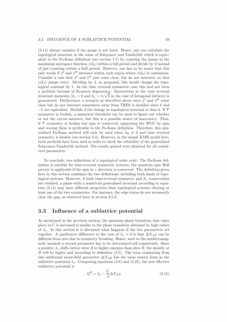
3.3. INFLUENCE OF A SUBLATTICE POTENTIAL 59
(3.14) always vanishes if the gauge is not fixed. Hence, one can calculate thetopological invariant in the sense of Soluyanov and Vanderbilt which is equiv-alent to the Fu-Kane definition (see section 1.7) by counting the jumps in themaximum interspace function z(k2) within a full period and divide by 2 insteadof just counting within a half period. However, one has to be aware that thisonly works if xI and xII intersect within each region where z(k2) is continuous.Consider a case that xI and xII just come close, but do not intersect, so thatz(k2) jumps twice. Dividing by 2, as proposed, this would change the topo-logical constant by 1. In the time reversal symmetric case this had not beena problem because of Kramers degeneracy: Intersection at the time reversalinvariant momenta (kx = 0 and kx = π/
√3 in the case of hexagonal lattices) is
guaranteed. Furthermore a scenario as described above were xI and xII comeclose but do not intersect somewhere away from TRIM is doubled since k and−k are equivalent. Modulo 2 the change in topological invariant is thus 0. If Tsymmetry is broken, a numerical threshold can be used to figure out whetheror not the curves intersect, but this is a possible source of inaccuracy. Thus,if T symmetry is broken but spin is conserved, separating the WCC by spinand tracing them is preferable to the Fu-Kane definition. Therefore, this gen-eralized Fu-Kane method will only be used when λR 6= 0 and time reversalsymmetry is broken (see section 3.4). However, in the simple KMH model here,both methods have been used in order to check the reliability of the generalizedSoluyanov-Vanderbilt method. The results gained were identical for all consid-ered parameters.
To conclude, two definitions of a topological order exist: The Fu-Kane def-inition is suitable for time-reversal symmetric systems, the quantum spin Hallpicture is applicable if the spin in z direction is conserved. The definition givenhere in this section combines the two definitions, including both kinds of topo-logical systems. However, if both time-reversal symmetry and Sz conservationare violated, a phase with a nontrivial generalised invariant according to equa-tion (3.14) may have different properties than topological systems obeying atleast one of the two symmetries. For instance, the edge states do not necessarilyclose the gap, as observed later in section 3.5.2.
3.3 Influence of a sublattice potential
As mentioned in the previous section, the quantum phase transition that takesplace as U is increased is similar to the phase transition obtained by high valuesof λν . In this section it is discussed what happens if the two parameters acttogether. A qualitative difference to the case of λν = 0 is that ∆NAB can bedifferent from zero due to symmetry breaking. Hence, next to the antiferromag-netic moment a second parameter has to be determined self consistently. Sincea positive λν shifts lattice sites A to higher energies than sites B, the density atB will be higher and according to definition (3.5). The term originating fromthis additional mean-field parameter ∆NAB has the same matrix form as thesublattice potential λν . Comparing equations (3.8) and (2.25), the new effectivesublattice potential is
λeffν = λν − U
4∆NAB (3.15)
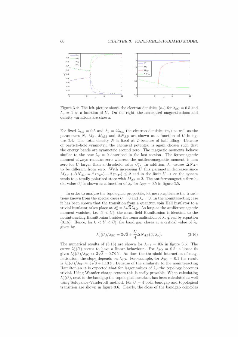
60 CHAPTER 3. KANE-MELE-HUBBARD MODEL
0 5 10 150
0.1
0.2
0.3
0.4
0.5
0.6
0.7
0.8
0.9
1
U
〈n〉
nA↑
nB↑
nA↓
nB↓
0 5 10 15−0.5
0
0.5
1
1.5
2
2.5
U
N
MF
MAF
∆NAB
Figure 3.4: The left picture shows the electron densities 〈nr〉 for λSO = 0.5 andλν = 1 as a function of U . On the right, the associated magnetisations anddensity variations are shown.
For fixed λSO = 0.5 and λν = 2λSO the electron densities 〈nr〉 as well as theparameters N , MF, MAM and ∆NAB are shown as a function of U in fig-ure 3.4. The total density N is fixed at 2 because of half filling. Becauseof particle-hole symmetry, the chemical potential is again chosen such thatthe energy bands are symmetric around zero. The magnetic moments behavesimilar to the case λν = 0 described in the last section. The ferromagneticmoment always remains zero whereas the antiferromagnetic moment is nonzero for U larger than a threshold value U c
1 . In addition, λν causes ∆NAB
to be different from zero. With increasing U this parameter decreases sinceMAF + ∆NAB = 2 〈nB↑〉 − 2 〈nA↑〉 ≤ 2 and in the limit U → ∞ the systemtends to a totally polarized state with MAF = 2. The antiferromagnetic thresh-old value U c
1 is shown as a function of λν for λSO = 0.5 in figure 3.5.
In order to analyse the topological properties, let me recapitulate the transi-tions known from the special cases U = 0 and λν = 0. In the noninteracting caseit has been shown that the transition from a quantum spin Hall insulator to atrivial insulator takes place at λcν = 3
√3λSO. As long as the antiferromagnetic
moment vanishes, i.e. U < U c1 , the mean-field Hamiltonian is identical to the
noninteracting Hamiltonian besides the renormalisation of λν given by equation(3.15). Hence, for 0 < U < U c
1 the band gap closes at a critical value of λνgiven by
λcν(U)/λSO = 3√3 +
U
4∆NAB(U, λν). (3.16)
The numerical results of (3.16) are shown for λSO = 0.5 in figure 3.5. Thecurve λcν(U) seems to have a linear behaviour. For λSO = 0.5, a linear fitgives λcν(U)/λSO ≈ 3
√3 + 0.78U . As does the threshold interaction of mag-
netisation, the slope depends on λSO. For example, for λSO = 0.1 the resultis λcν(U)/λSO ≈ 3
√3 + 1.13U . Because of the similarity to the noninteracting
Hamiltonian it is expected that for larger values of λν the topology becomestrivial. Using Wannier charge centers this is easily provable. When calculatingλcν(U), next to the bandgap the topological invariant has been calculated as wellusing Soluyanov-Vanderbilt method. For U = 4 both bandgap and topologicaltransition are shown in figure 3.6. Clearly, the close of the bandgap coincides
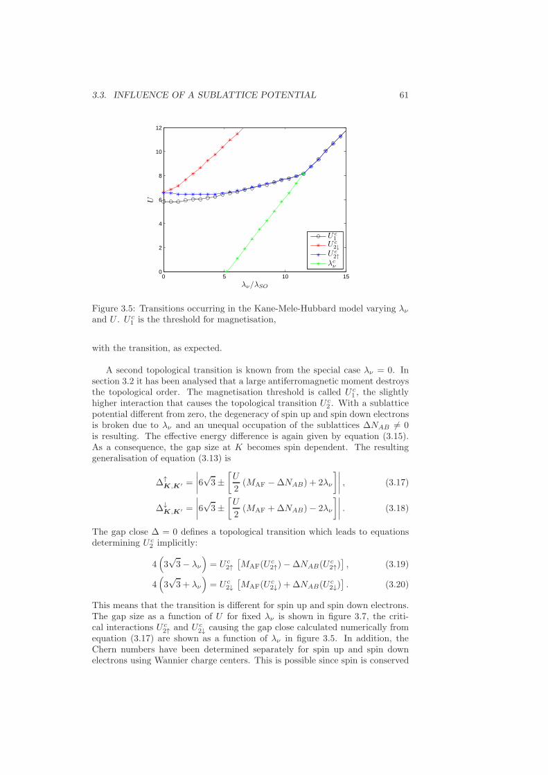
3.3. INFLUENCE OF A SUBLATTICE POTENTIAL 61
0 5 10 150
2
4
6
8
10
12
λν/λSO
U
U c1
U c2↓
U c2↑
λcν
Figure 3.5: Transitions occurring in the Kane-Mele-Hubbard model varying λνand U . U c
1 is the threshold for magnetisation,
with the transition, as expected.
A second topological transition is known from the special case λν = 0. Insection 3.2 it has been analysed that a large antiferromagnetic moment destroysthe topological order. The magnetisation threshold is called U c
1 , the slightlyhigher interaction that causes the topological transition U c
2 . With a sublatticepotential different from zero, the degeneracy of spin up and spin down electronsis broken due to λν and an unequal occupation of the sublattices ∆NAB 6= 0is resulting. The effective energy difference is again given by equation (3.15).As a consequence, the gap size at K becomes spin dependent. The resultinggeneralisation of equation (3.13) is
∆↑K,K′ =
∣∣∣∣6√3±
[U
2(MAF −∆NAB) + 2λν
]∣∣∣∣ , (3.17)
∆↓K,K′ =
∣∣∣∣6√3±
[U
2(MAF +∆NAB)− 2λν
]∣∣∣∣ . (3.18)
The gap close ∆ = 0 defines a topological transition which leads to equationsdetermining U c
2 implicitly:
4(3√3− λν
)= U c
2↑[MAF(U
c2↑)−∆NAB(U
c2↑)], (3.19)
4(3√3 + λν
)= U c
2↓[MAF(U
c2↓) + ∆NAB(U
c2↓)]. (3.20)
This means that the transition is different for spin up and spin down electrons.The gap size as a function of U for fixed λν is shown in figure 3.7, the criti-cal interactions U c
2↑ and U c2↓ causing the gap close calculated numerically from
equation (3.17) are shown as a function of λν in figure 3.5. In addition, theChern numbers have been determined separately for spin up and spin downelectrons using Wannier charge centers. This is possible since spin is conserved
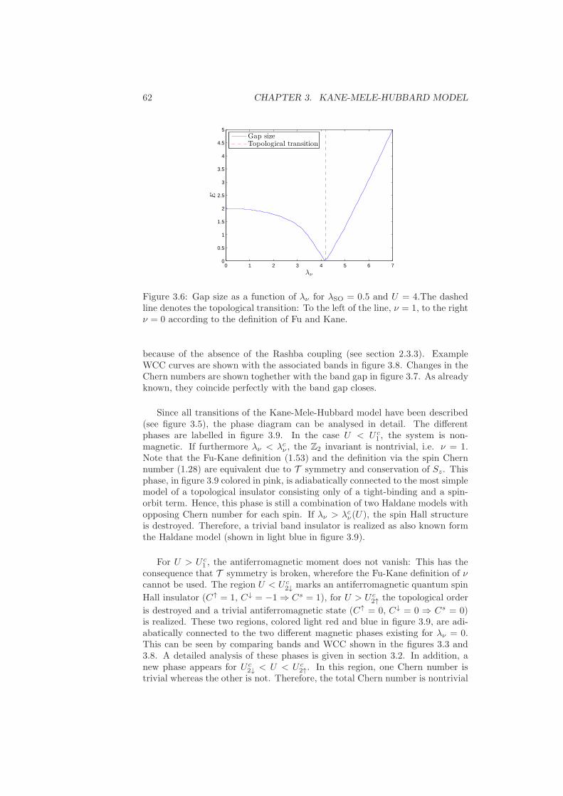
62 CHAPTER 3. KANE-MELE-HUBBARD MODEL
0 1 2 3 4 5 6 70
0.5
1
1.5
2
2.5
3
3.5
4
4.5
5
λν
E
Gap sizeTopological transition
Figure 3.6: Gap size as a function of λν for λSO = 0.5 and U = 4.The dashedline denotes the topological transition: To the left of the line, ν = 1, to the rightν = 0 according to the definition of Fu and Kane.
because of the absence of the Rashba coupling (see section 2.3.3). ExampleWCC curves are shown with the associated bands in figure 3.8. Changes in theChern numbers are shown toghether with the band gap in figure 3.7. As alreadyknown, they coincide perfectly with the band gap closes.
Since all transitions of the Kane-Mele-Hubbard model have been described(see figure 3.5), the phase diagram can be analysed in detail. The differentphases are labelled in figure 3.9. In the case U < U c
1 , the system is non-magnetic. If furthermore λν < λcν , the Z2 invariant is nontrivial, i.e. ν = 1.Note that the Fu-Kane definition (1.53) and the definition via the spin Chernnumber (1.28) are equivalent due to T symmetry and conservation of Sz. Thisphase, in figure 3.9 colored in pink, is adiabatically connected to the most simplemodel of a topological insulator consisting only of a tight-binding and a spin-orbit term. Hence, this phase is still a combination of two Haldane models withopposing Chern number for each spin. If λν > λcν(U), the spin Hall structureis destroyed. Therefore, a trivial band insulator is realized as also known formthe Haldane model (shown in light blue in figure 3.9).
For U > U c1 , the antiferromagnetic moment does not vanish: This has the
consequence that T symmetry is broken, wherefore the Fu-Kane definition of νcannot be used. The region U < U c
2↓ marks an antiferromagnetic quantum spin
Hall insulator (C↑ = 1, C↓ = −1 ⇒ Cs = 1), for U > U c2↑ the topological order
is destroyed and a trivial antiferromagnetic state (C↑ = 0, C↓ = 0 ⇒ Cs = 0)is realized. These two regions, colored light red and blue in figure 3.9, are adi-abatically connected to the two different magnetic phases existing for λν = 0.This can be seen by comparing bands and WCC shown in the figures 3.3 and3.8. A detailed analysis of these phases is given in section 3.2. In addition, anew phase appears for U c
2↓ < U < U c2↑. In this region, one Chern number is
trivial whereas the other is not. Therefore, the total Chern number is nontrivial
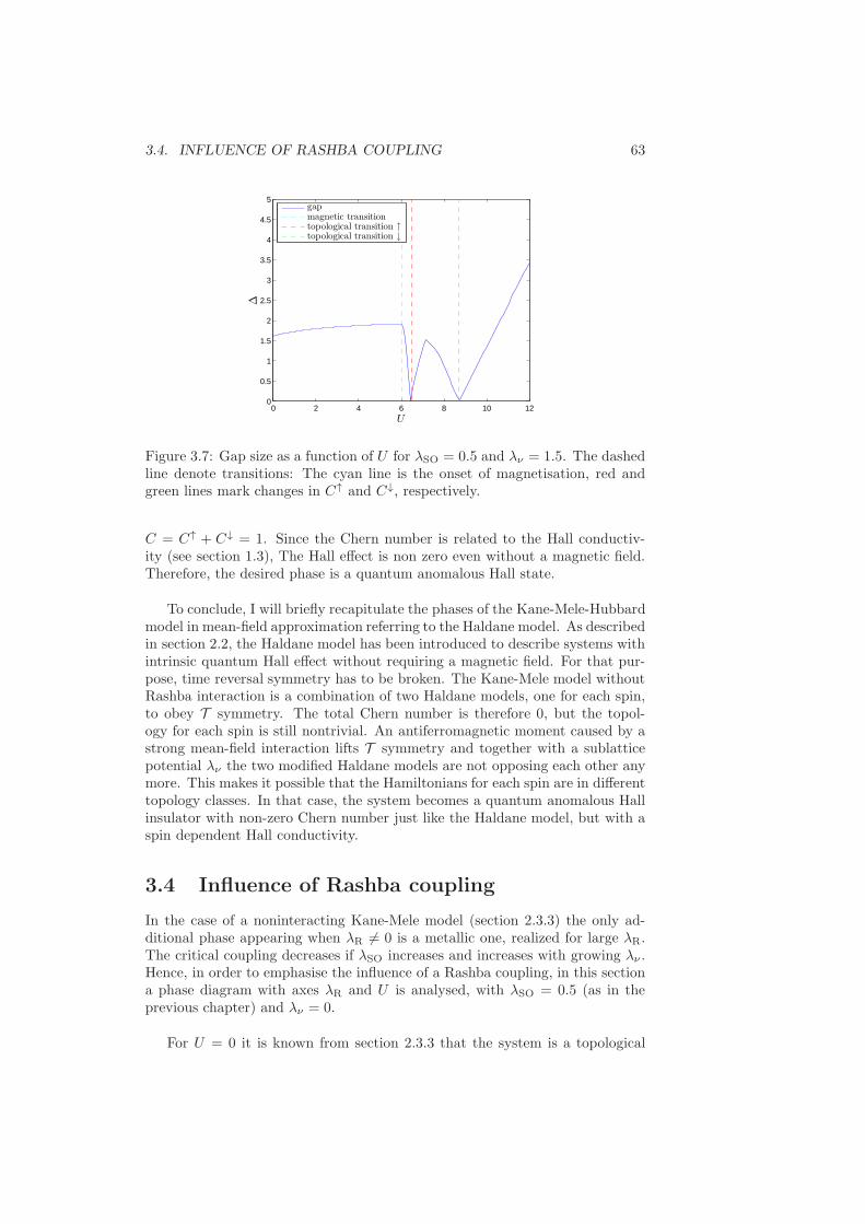
3.4. INFLUENCE OF RASHBA COUPLING 63
0 2 4 6 8 10 120
0.5
1
1.5
2
2.5
3
3.5
4
4.5
5
U
∆
gapmagnetic transitiontopological transition ↑topological transition ↓
Figure 3.7: Gap size as a function of U for λSO = 0.5 and λν = 1.5. The dashedline denote transitions: The cyan line is the onset of magnetisation, red andgreen lines mark changes in C↑ and C↓, respectively.
C = C↑ + C↓ = 1. Since the Chern number is related to the Hall conductiv-ity (see section 1.3), The Hall effect is non zero even without a magnetic field.Therefore, the desired phase is a quantum anomalous Hall state.
To conclude, I will briefly recapitulate the phases of the Kane-Mele-Hubbardmodel in mean-field approximation referring to the Haldane model. As describedin section 2.2, the Haldane model has been introduced to describe systems withintrinsic quantum Hall effect without requiring a magnetic field. For that pur-pose, time reversal symmetry has to be broken. The Kane-Mele model withoutRashba interaction is a combination of two Haldane models, one for each spin,to obey T symmetry. The total Chern number is therefore 0, but the topol-ogy for each spin is still nontrivial. An antiferromagnetic moment caused by astrong mean-field interaction lifts T symmetry and together with a sublatticepotential λν the two modified Haldane models are not opposing each other anymore. This makes it possible that the Hamiltonians for each spin are in differenttopology classes. In that case, the system becomes a quantum anomalous Hallinsulator with non-zero Chern number just like the Haldane model, but with aspin dependent Hall conductivity.
3.4 Influence of Rashba coupling
In the case of a noninteracting Kane-Mele model (section 2.3.3) the only ad-ditional phase appearing when λR 6= 0 is a metallic one, realized for large λR.The critical coupling decreases if λSO increases and increases with growing λν .Hence, in order to emphasise the influence of a Rashba coupling, in this sectiona phase diagram with axes λR and U is analysed, with λSO = 0.5 (as in theprevious chapter) and λν = 0.
For U = 0 it is known from section 2.3.3 that the system is a topological
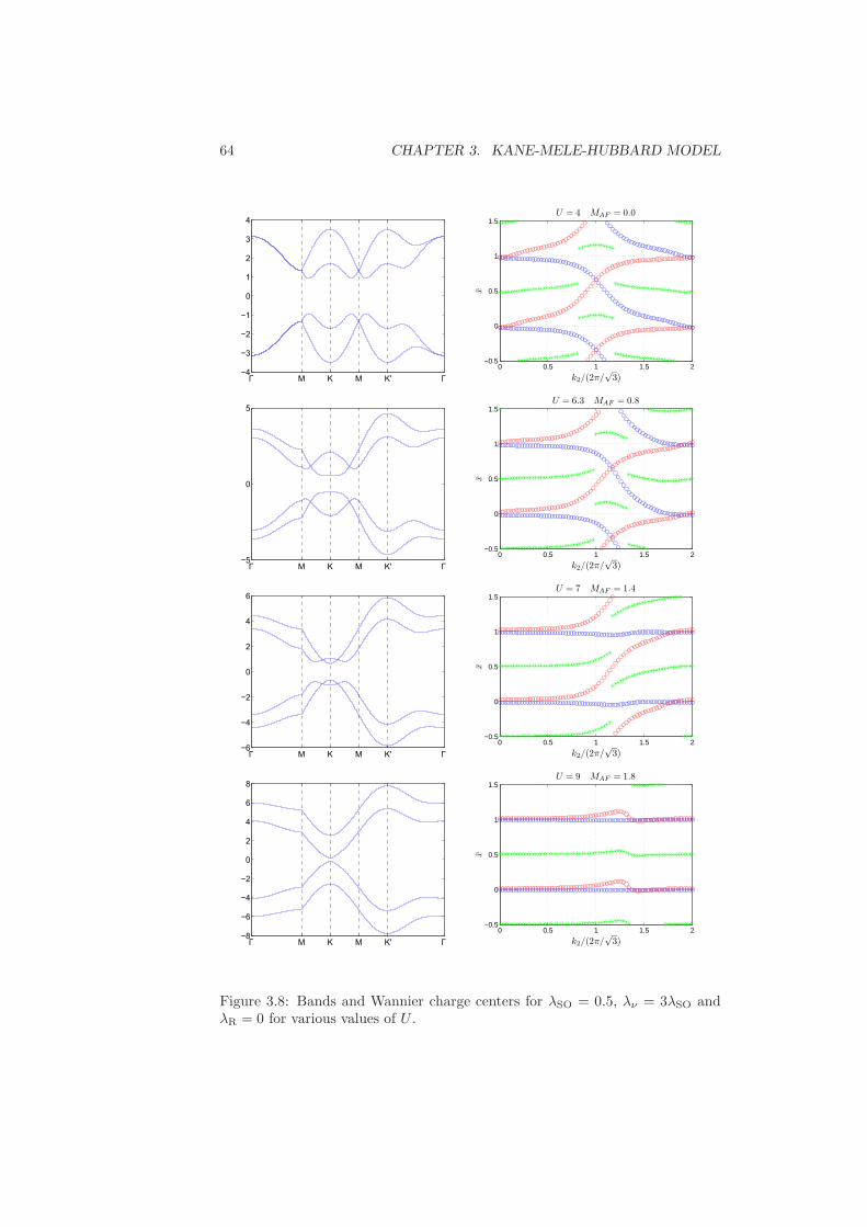
64 CHAPTER 3. KANE-MELE-HUBBARD MODEL
0 0.5 1 1.5 2−0.5
0
0.5
1
1.5
x
k2/(2π/√
3)
U = 4 MAF = 0.0
0 0.5 1 1.5 2−0.5
0
0.5
1
1.5
x
k2/(2π/√
3)
U = 6.3 MAF = 0.8
0 0.5 1 1.5 2−0.5
0
0.5
1
1.5
x
k2/(2π/√
3)
U = 7 MAF = 1.4
0 0.5 1 1.5 2−0.5
0
0.5
1
1.5
x
k2/(2π/√
3)
U = 9 MAF = 1.8
Figure 3.8: Bands and Wannier charge centers for λSO = 0.5, λν = 3λSO andλR = 0 for various values of U .
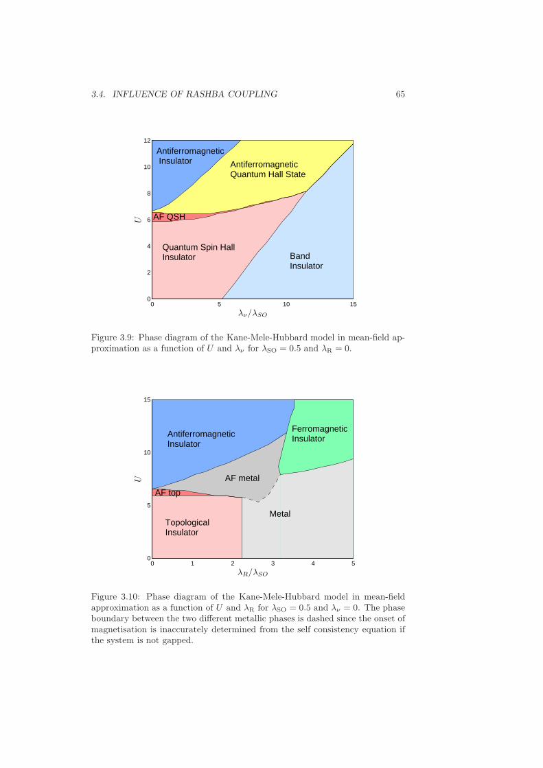
3.4. INFLUENCE OF RASHBA COUPLING 65
0 5 10 150
2
4
6
8
10
12
λν/λSO
U
BandInsulator
Quantum Spin HallInsulator
AF QSH
Antiferromagnetic Insulator Antiferromagnetic
Quantum Hall State
Figure 3.9: Phase diagram of the Kane-Mele-Hubbard model in mean-field ap-proximation as a function of U and λν for λSO = 0.5 and λR = 0.
0 1 2 3 4 50
5
10
15
λR/λSO
U
AntiferromagneticInsulator
AF metal
Metal
FerromagneticInsulator
TopologicalInsulator
AF top
Figure 3.10: Phase diagram of the Kane-Mele-Hubbard model in mean-fieldapproximation as a function of U and λR for λSO = 0.5 and λν = 0. The phaseboundary between the two different metallic phases is dashed since the onset ofmagnetisation is inaccurately determined from the self consistency equation ifthe system is not gapped.
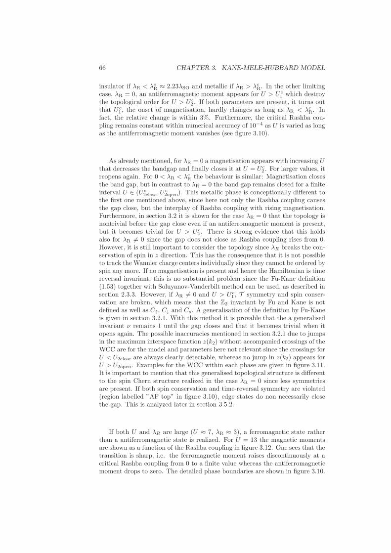
66 CHAPTER 3. KANE-MELE-HUBBARD MODEL
insulator if λR < λcR ≈ 2.23λSO and metallic if λR > λcR. In the other limitingcase, λR = 0, an antiferromagnetic moment appears for U > U c
1 which destroythe topological order for U > U c
2 . If both parameters are present, it turns outthat U c
1 , the onset of magnetisation, hardly changes as long as λR < λcR. Infact, the relative change is within 3%. Furthermore, the critical Rashba cou-pling remains constant within numerical accuracy of 10−4 as U is varied as longas the antiferromagnetic moment vanishes (see figure 3.10).
As already mentioned, for λR = 0 a magnetisation appears with increasing Uthat decreases the bandgap and finally closes it at U = U c
2 . For larger values, itreopens again. For 0 < λR < λcR the behaviour is similar: Magnetisation closesthe band gap, but in contrast to λR = 0 the band gap remains closed for a finiteinterval U ∈ (U c
2close, Uc2open). This metallic phase is conceptionally different to
the first one mentioned above, since here not only the Rashba coupling causesthe gap close, but the interplay of Rashba coupling with rising magnetisation.Furthermore, in section 3.2 it is shown for the case λR = 0 that the topology isnontrivial before the gap close even if an antiferromagnetic moment is present,but it becomes trivial for U > U c
2 . There is strong evidence that this holdsalso for λR 6= 0 since the gap does not close as Rashba coupling rises from 0.However, it is still important to consider the topology since λR breaks the con-servation of spin in z direction. This has the consequence that it is not possibleto track the Wannier charge centers individually since they cannot be ordered byspin any more. If no magnetisation is present and hence the Hamiltonian is timereversal invariant, this is no substantial problem since the Fu-Kane definition(1.53) together with Soluyanov-Vanderbilt method can be used, as described insection 2.3.3. However, if λR 6= 0 and U > U c
1 , T symmetry and spin conser-vation are broken, which means that the Z2 invariant by Fu and Kane is notdefined as well as C↑, C↓ and Cs. A generalisation of the definition by Fu-Kaneis given in section 3.2.1. With this method it is provable that the a generalisedinvariant ν remains 1 until the gap closes and that it becomes trivial when itopens again. The possible inaccuracies mentioned in section 3.2.1 due to jumpsin the maximum interspace function z(k2) without accompanied crossings of theWCC are for the model and parameters here not relevant since the crossings forU < U2close are always clearly detectable, whereas no jump in z(k2) appears forU > U2open. Examples for the WCC within each phase are given in figure 3.11.It is important to mention that this generalised topological structure is differentto the spin Chern structure realized in the case λR = 0 since less symmetriesare present. If both spin conservation and time-reversal symmetry are violated(region labelled ”AF top” in figure 3.10), edge states do non necessarily closethe gap. This is analyzed later in section 3.5.2.
If both U and λR are large (U ≈ 7, λR ≈ 3), a ferromagnetic state ratherthan a antiferromagnetic state is realized. For U = 13 the magnetic momentsare shown as a function of the Rashba coupling in figure 3.12. One sees that thetransition is sharp, i.e. the ferromagnetic moment raises discontinuously at acritical Rashba coupling from 0 to a finite value whereas the antiferromagneticmoment drops to zero. The detailed phase boundaries are shown in figure 3.10.
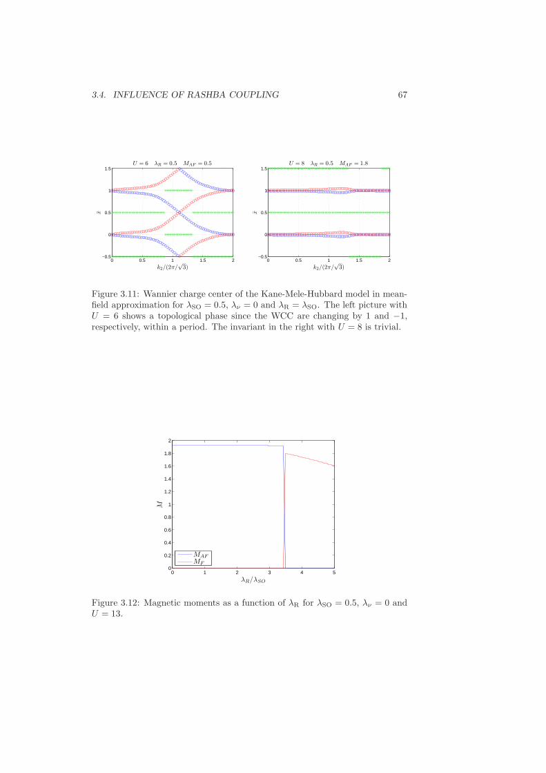
3.4. INFLUENCE OF RASHBA COUPLING 67
0 0.5 1 1.5 2−0.5
0
0.5
1
1.5
x
k2/(2π/√
3)
U = 6 λR = 0.5 MAF = 0.5
0 0.5 1 1.5 2−0.5
0
0.5
1
1.5
x
k2/(2π/√
3)
U = 8 λR = 0.5 MAF = 1.8
Figure 3.11: Wannier charge center of the Kane-Mele-Hubbard model in mean-field approximation for λSO = 0.5, λν = 0 and λR = λSO. The left picture withU = 6 shows a topological phase since the WCC are changing by 1 and −1,respectively, within a period. The invariant in the right with U = 8 is trivial.
0 1 2 3 4 50
0.2
0.4
0.6
0.8
1
1.2
1.4
1.6
1.8
2
λR/λSO
M
MAF
MF
Figure 3.12: Magnetic moments as a function of λR for λSO = 0.5, λν = 0 andU = 13.
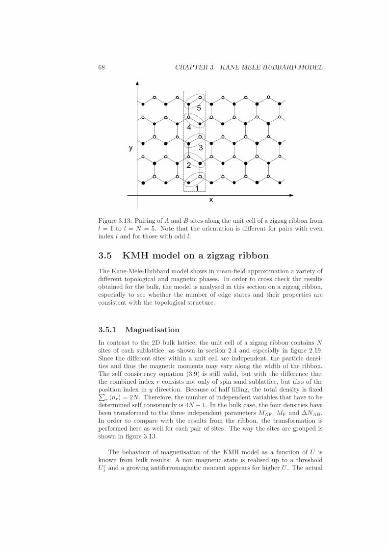
68 CHAPTER 3. KANE-MELE-HUBBARD MODEL
Figure 3.13: Pairing of A and B sites along the unit cell of a zigzag ribbon froml = 1 to l = N = 5. Note that the orientation is different for pairs with evenindex l and for those with odd l.
3.5 KMH model on a zigzag ribbon
The Kane-Mele-Hubbard model shows in mean-field approximation a variety ofdifferent topological and magnetic phases. In order to cross check the resultsobtained for the bulk, the model is analysed in this section on a zigzag ribbon,especially to see whether the number of edge states and their properties areconsistent with the topological structure.
3.5.1 Magnetisation
In contrast to the 2D bulk lattice, the unit cell of a zigzag ribbon contains Nsites of each sublattice, as shown in section 2.4 and especially in figure 2.19.Since the different sites within a unit cell are independent, the particle densi-ties and thus the magnetic moments may vary along the width of the ribbon.The self consistency equation (3.9) is still valid, but with the difference thatthe combined index r consists not only of spin sand sublattice, but also of theposition index in y direction. Because of half filling, the total density is fixed∑
r 〈nr〉 = 2N . Therefore, the number of independent variables that have to bedetermined self consistently is 4N − 1. In the bulk case, the four densities havebeen transformed to the three independent parameters MAF, MF and ∆NAB.In order to compare with the results from the ribbon, the transformation isperformed here as well for each pair of sites. The way the sites are grouped isshown in figure 3.13.
The behaviour of magnetisation of the KMH model as a function of U isknown from bulk results: A non magnetic state is realised up to a thresholdU c1 and a growing antiferromagnetic moment appears for higher U . The actual
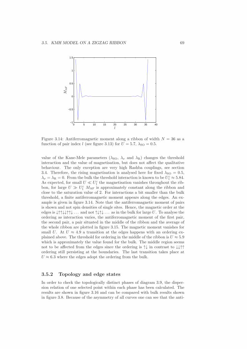
3.5. KMH MODEL ON A ZIGZAG RIBBON 69
0 5 10 15 20 25 30 35 40−1
−0.5
0
0.5
1
1.5
l
MA
F
Figure 3.14: Antiferromagnetic moment along a ribbon of width N = 36 as afunction of pair index l (see figure 3.13) for U = 5.7, λSO = 0.5.
value of the Kane-Mele parameters (λSO, λν and λR) changes the thresholdinteraction and the value of magnetisation, but does not affect the qualitativebehaviour. The only exception are very high Rashba couplings, see section3.4. Therefore, the rising magnetisation is analysed here for fixed λSO = 0.5,λν = λR = 0. From the bulk the threshold interaction is known to be U c
1 ≈ 5.84.As expected, for small U ≪ U c
1 the magnetisation vanishes throughout the rib-bon, for large U ≫ U c
1 MAF is approximately constant along the ribbon andclose to the saturation value of 2. For interactions a bit smaller than the bulkthreshold, a finite antiferromagnetic moment appears along the edges. An ex-ample is given in figure 3.14. Note that the antiferromagnetic moment of pairsis shown and not spin densities of single sites. Hence, the magnetic order at theedges is ↓↑↑↓↓↑↑↓ . . . and not ↑↓↑↓ . . . as in the bulk for large U . To analyse theordering as interaction varies, the antiferromagnetic moment of the first pair,the second pair, a pair situated in the middle of the ribbon and the average ofthe whole ribbon are plotted in figure 3.15. The magnetic moment vanishes forsmall U . At U ≈ 4.9 a transition at the edges happens with an ordering ex-plained above. The threshold for ordering in the middle of the ribbon is U ≈ 5.9which is approximately the value found for the bulk. The middle region seemsnot to be affected from the edges since the ordering is ↑↓ in contrast to ↓↓↑↑ordering still persisting at the boundaries. The last transition takes place atU ≈ 6.3 where the edges adopt the ordering from the bulk.
3.5.2 Topology and edge states
In order to check the topologically distinct phases of diagram 3.9, the disper-sion relation of one selected point within each phase has been calculated. Theresults are shown in figure 3.16 and can be compared with bulk results shownin figure 3.8. Because of the asymmetry of all curves one can see that the anti-
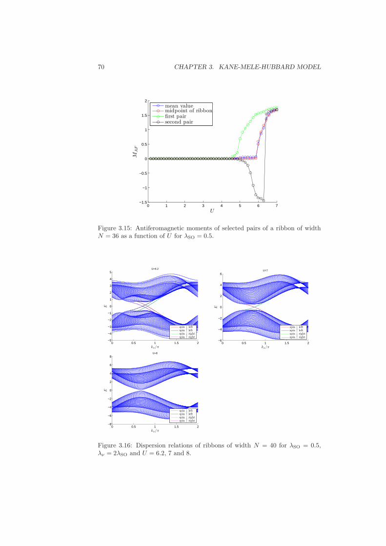
70 CHAPTER 3. KANE-MELE-HUBBARD MODEL
0 1 2 3 4 5 6 7−1.5
−1
−0.5
0
0.5
1
1.5
2
U
MA
F
mean valuemidpoint of ribbonfirst pairsecond pair
Figure 3.15: Antiferomagnetic moments of selected pairs of a ribbon of widthN = 36 as a function of U for λSO = 0.5.
0 0.5 1 1.5 2−5
−4
−3
−2
−1
0
1
2
3
4
5
kx/π
E
U=6.2
spin ↓ leftspin ↑ leftspin ↓ rightspin ↑ right
0 0.5 1 1.5 2−6
−4
−2
0
2
4
6
kx/π
E
U=7
spin ↓ leftspin ↑ leftspin ↓ rightspin ↑ right
0 0.5 1 1.5 2−8
−6
−4
−2
0
2
4
6
8
kx/π
E
U=8
spin ↓ leftspin ↑ leftspin ↓ rightspin ↑ right
Figure 3.16: Dispersion relations of ribbons of width N = 40 for λSO = 0.5,λν = 2λSO and U = 6.2, 7 and 8.
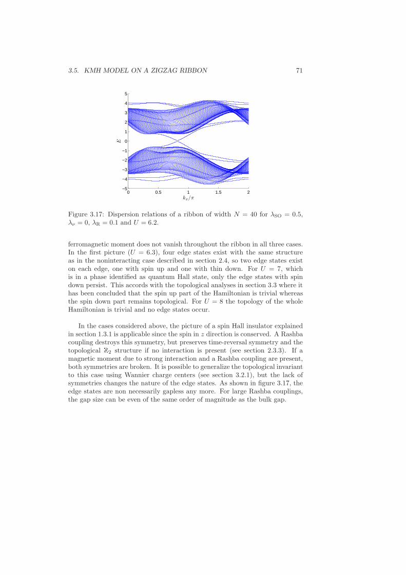
3.5. KMH MODEL ON A ZIGZAG RIBBON 71
0 0.5 1 1.5 2−5
−4
−3
−2
−1
0
1
2
3
4
5
kx/π
E
Figure 3.17: Dispersion relations of a ribbon of width N = 40 for λSO = 0.5,λν = 0, λR = 0.1 and U = 6.2.
ferromagnetic moment does not vanish throughout the ribbon in all three cases.In the first picture (U = 6.3), four edge states exist with the same structureas in the noninteracting case described in section 2.4, so two edge states existon each edge, one with spin up and one with thin down. For U = 7, whichis in a phase identified as quantum Hall state, only the edge states with spindown persist. This accords with the topological analyses in section 3.3 where ithas been concluded that the spin up part of the Hamiltonian is trivial whereasthe spin down part remains topological. For U = 8 the topology of the wholeHamiltonian is trivial and no edge states occur.
In the cases considered above, the picture of a spin Hall insulator explainedin section 1.3.1 is applicable since the spin in z direction is conserved. A Rashbacoupling destroys this symmetry, but preserves time-reversal symmetry and thetopological Z2 structure if no interaction is present (see section 2.3.3). If amagnetic moment due to strong interaction and a Rashba coupling are present,both symmetries are broken. It is possible to generalize the topological invariantto this case using Wannier charge centers (see section 3.2.1), but the lack ofsymmetries changes the nature of the edge states. As shown in figure 3.17, theedge states are non necessarily gapless any more. For large Rashba couplings,the gap size can be even of the same order of magnitude as the bulk gap.

72 CHAPTER 3. KANE-MELE-HUBBARD MODEL
Chapter 4
Kane-Mele-Hubbard model
beyond mean-field
approximation
As mentioned in the previous chapter, the KMH model is a good system in orderto understand the influence of interactions on topology. It is thus also expectedto work as a toy model to test the advanced methods to determine topologicalconstants explained in section 1.8. Therefore, it has been investigated by severalmethods after Rachel and Le Hur [48] first considered this model in mean-field approximation. The the critical U for a finite magnetisation has beenexamined for example with a determinant quantum Monte Carlo [49] as wellas with a cellular dynamical mean-field theory [50]. The Variational ClusterApproach has also been used in order to determine the phases [50–52]. In thetwo latter references, the obtained Green’s function of the inversion symmetricmodel is used to determine topological phases with equation (1.77). The aimof this chapter is to use also a self-energy-functional based method to calculatetopological invariants even if inversion symmetry is broken, to look whetherthe topologically nontrivial phases with antiferromagnetic moment described inchapter 2 persist beyond mean-field approximation.
4.1 Self-energy-functional approach
Consider a Hamiltonian H = H0(t) + H1(U) consisting of a noninteractingpart depending on a hopping matrix t and an interacting one depending on aninteraction tensor U ,
H =∑
ij
tijc†i cj +
1
2
∑
ijkl
Uijklc†i c
†jclck. (4.1)
The Green’s function of H0 is given by G0 = 1/(ω + µ − t) and determinestogether with the self-energy Σ the full Green’s function G via the Dyson equa-tion G = G0 +G0ΣG (see for example [47]). In contrast to the free Green’sfunction, the self-energy is not known beforehand and can usually only be calcu-lated approximately. In the following, the self-energy-functional approach [53]
73
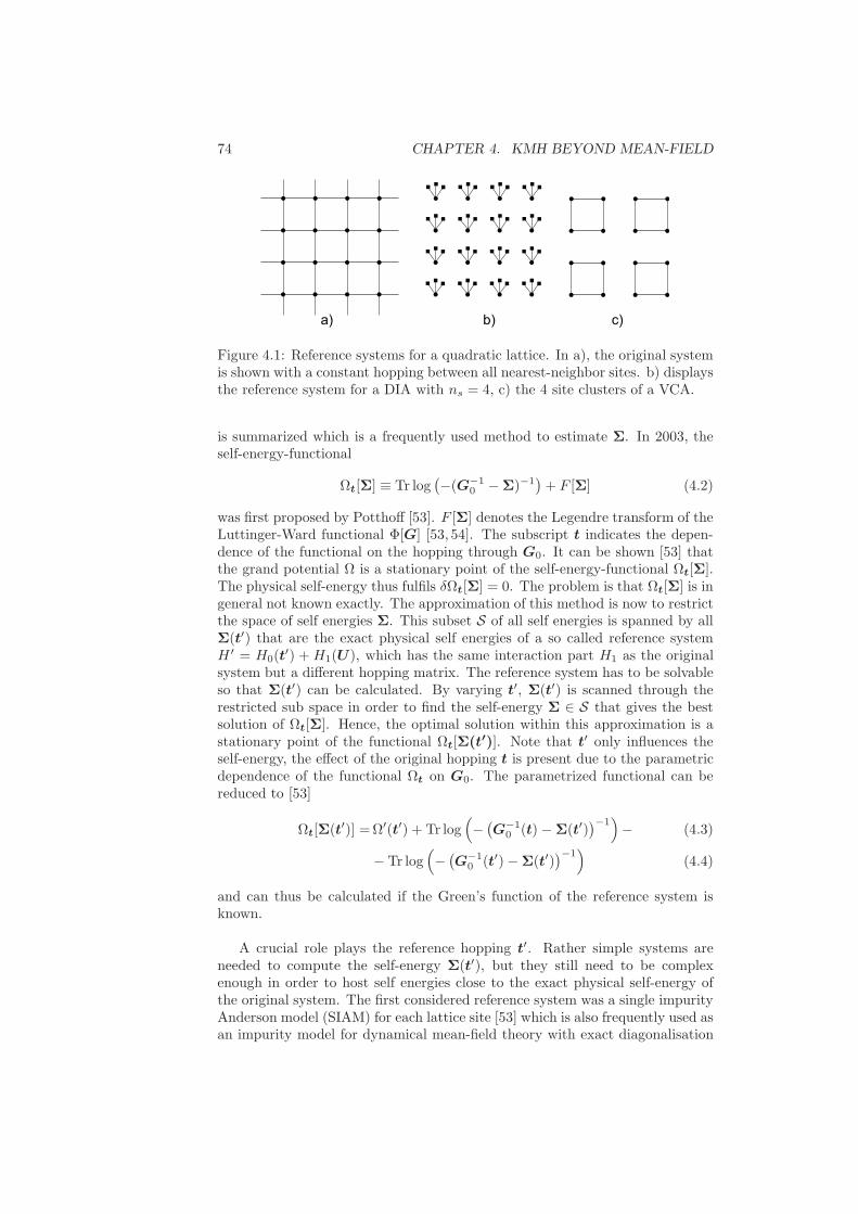
74 CHAPTER 4. KMH BEYOND MEAN-FIELD
Figure 4.1: Reference systems for a quadratic lattice. In a), the original systemis shown with a constant hopping between all nearest-neighbor sites. b) displaysthe reference system for a DIA with ns = 4, c) the 4 site clusters of a VCA.
is summarized which is a frequently used method to estimate Σ. In 2003, theself-energy-functional
Ωt[Σ] ≡ Tr log(−(G−1
0 −Σ)−1)+ F [Σ] (4.2)
was first proposed by Potthoff [53]. F [Σ] denotes the Legendre transform of theLuttinger-Ward functional Φ[G] [53, 54]. The subscript t indicates the depen-dence of the functional on the hopping through G0. It can be shown [53] thatthe grand potential Ω is a stationary point of the self-energy-functional Ωt[Σ].The physical self-energy thus fulfils δΩt[Σ] = 0. The problem is that Ωt[Σ] is ingeneral not known exactly. The approximation of this method is now to restrictthe space of self energies Σ. This subset S of all self energies is spanned by allΣ(t′) that are the exact physical self energies of a so called reference systemH ′ = H0(t
′) +H1(U), which has the same interaction part H1 as the originalsystem but a different hopping matrix. The reference system has to be solvableso that Σ(t′) can be calculated. By varying t′, Σ(t′) is scanned through therestricted sub space in order to find the self-energy Σ ∈ S that gives the bestsolution of Ωt[Σ]. Hence, the optimal solution within this approximation is astationary point of the functional Ωt[Σ(t′)]. Note that t′ only influences theself-energy, the effect of the original hopping t is present due to the parametricdependence of the functional Ωt on G0. The parametrized functional can bereduced to [53]
Ωt[Σ(t′)] =Ω′(t′) + Tr log(−(G−1
0 (t) −Σ(t′))−1)− (4.3)
− Tr log(−(G−1
0 (t′)−Σ(t′))−1)
(4.4)
and can thus be calculated if the Green’s function of the reference system isknown.
A crucial role plays the reference hopping t′. Rather simple systems areneeded to compute the self-energy Σ(t′), but they still need to be complexenough in order to host self energies close to the exact physical self-energy ofthe original system. The first considered reference system was a single impurityAnderson model (SIAM) for each lattice site [53] which is also frequently used asan impurity model for dynamical mean-field theory with exact diagonalisation
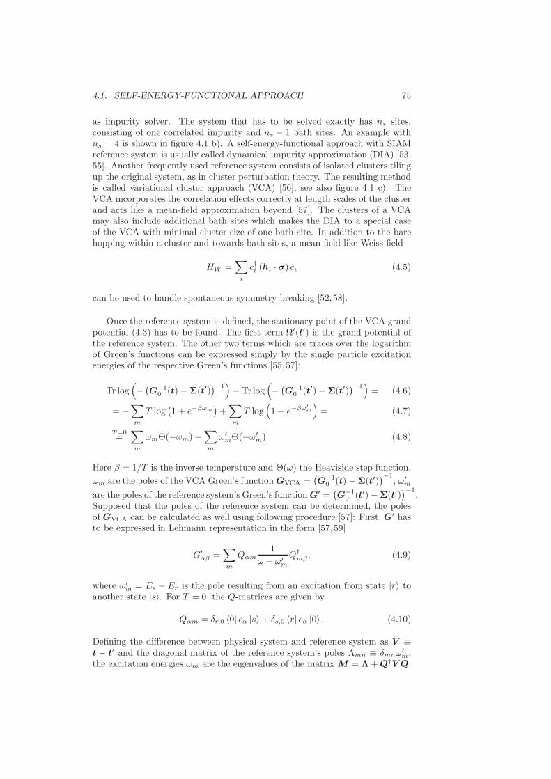
4.1. SELF-ENERGY-FUNCTIONAL APPROACH 75
as impurity solver. The system that has to be solved exactly has ns sites,consisting of one correlated impurity and ns − 1 bath sites. An example withns = 4 is shown in figure 4.1 b). A self-energy-functional approach with SIAMreference system is usually called dynamical impurity approximation (DIA) [53,55]. Another frequently used reference system consists of isolated clusters tilingup the original system, as in cluster perturbation theory. The resulting methodis called variational cluster approach (VCA) [56], see also figure 4.1 c). TheVCA incorporates the correlation effects correctly at length scales of the clusterand acts like a mean-field approximation beyond [57]. The clusters of a VCAmay also include additional bath sites which makes the DIA to a special caseof the VCA with minimal cluster size of one bath site. In addition to the barehopping within a cluster and towards bath sites, a mean-field like Weiss field
HW =∑
i
c†i (hi · σ) ci (4.5)
can be used to handle spontaneous symmetry breaking [52, 58].
Once the reference system is defined, the stationary point of the VCA grandpotential (4.3) has to be found. The first term Ω′(t′) is the grand potential ofthe reference system. The other two terms which are traces over the logarithmof Green’s functions can be expressed simply by the single particle excitationenergies of the respective Green’s functions [55, 57]:
Tr log(−(G−1
0 (t) −Σ(t′))−1)− Tr log
(−(G−1
0 (t′)−Σ(t′))−1)= (4.6)
= −∑
m
T log(1 + e−βωm
)+∑
m
T log(1 + e−βω′
m
)= (4.7)
T=0=
∑
m
ωmΘ(−ωm)−∑
m
ω′mΘ(−ω′
m). (4.8)
Here β = 1/T is the inverse temperature and Θ(ω) the Heaviside step function.
ωm are the poles of the VCA Green’s function GVCA =(G−1
0 (t) −Σ(t′))−1
, ω′m
are the poles of the reference system’s Green’s functionG′ =(G−1
0 (t′)−Σ(t′))−1
.Supposed that the poles of the reference system can be determined, the polesof GVCA can be calculated as well using following procedure [57]: First, G′ hasto be expressed in Lehmann representation in the form [57, 59]
G′αβ =
∑
m
Qαm1
ω − ω′m
Q†mβ, (4.9)
where ω′m = Es − Er is the pole resulting from an excitation from state |r〉 to
another state |s〉. For T = 0, the Q-matrices are given by
Qαm = δr,0 〈0| cα |s〉+ δs,0 〈r| cα |0〉 . (4.10)
Defining the difference between physical system and reference system as V ≡t − t′ and the diagonal matrix of the reference system’s poles Λmn ≡ δmnω
′m,
the excitation energies ωm are the eigenvalues of the matrix M = Λ+Q†V Q.
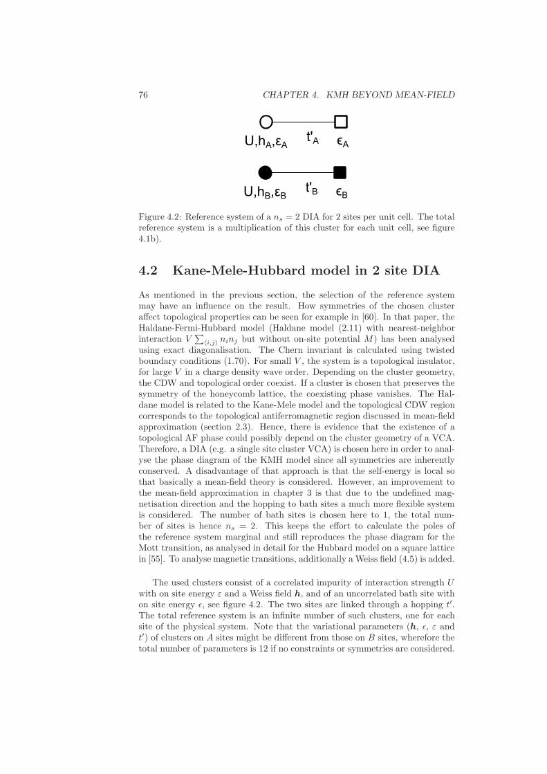
76 CHAPTER 4. KMH BEYOND MEAN-FIELD
Figure 4.2: Reference system of a ns = 2 DIA for 2 sites per unit cell. The totalreference system is a multiplication of this cluster for each unit cell, see figure4.1b).
4.2 Kane-Mele-Hubbard model in 2 site DIA
As mentioned in the previous section, the selection of the reference systemmay have an influence on the result. How symmetries of the chosen clusteraffect topological properties can be seen for example in [60]. In that paper, theHaldane-Fermi-Hubbard model (Haldane model (2.11) with nearest-neighborinteraction V
∑〈i,j〉 ninj but without on-site potential M) has been analysed
using exact diagonalisation. The Chern invariant is calculated using twistedboundary conditions (1.70). For small V , the system is a topological insulator,for large V in a charge density wave order. Depending on the cluster geometry,the CDW and topological order coexist. If a cluster is chosen that preserves thesymmetry of the honeycomb lattice, the coexisting phase vanishes. The Hal-dane model is related to the Kane-Mele model and the topological CDW regioncorresponds to the topological antiferromagnetic region discussed in mean-fieldapproximation (section 2.3). Hence, there is evidence that the existence of atopological AF phase could possibly depend on the cluster geometry of a VCA.Therefore, a DIA (e.g. a single site cluster VCA) is chosen here in order to anal-yse the phase diagram of the KMH model since all symmetries are inherentlyconserved. A disadvantage of that approach is that the self-energy is local sothat basically a mean-field theory is considered. However, an improvement tothe mean-field approximation in chapter 3 is that due to the undefined mag-netisation direction and the hopping to bath sites a much more flexible systemis considered. The number of bath sites is chosen here to 1, the total num-ber of sites is hence ns = 2. This keeps the effort to calculate the poles ofthe reference system marginal and still reproduces the phase diagram for theMott transition, as analysed in detail for the Hubbard model on a square latticein [55]. To analyse magnetic transitions, additionally a Weiss field (4.5) is added.
The used clusters consist of a correlated impurity of interaction strength Uwith on site energy ε and a Weiss field h, and of an uncorrelated bath site withon site energy ǫ, see figure 4.2. The two sites are linked through a hopping t′.The total reference system is an infinite number of such clusters, one for eachsite of the physical system. Note that the variational parameters (h, ǫ, ε andt′) of clusters on A sites might be different from those on B sites, wherefore thetotal number of parameters is 12 if no constraints or symmetries are considered.
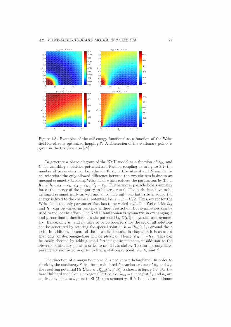
4.2. KANE-MELE-HUBBARD MODEL IN 2 SITE DIA 77
0 0.5 1 1.5 20
0.2
0.4
0.6
0.8
1
1.2
1.4
1.6
1.8
2 λSO = 0 U = 5.5
hx
hz
−6.43
−6.425
−6.42
−6.415
−6.41
−6.405
−6.4
−6.395
−6.39
−6.385
−6.38
0 0.5 1 1.5 20
0.2
0.4
0.6
0.8
1
1.2
1.4
1.6
1.8
2 λSO = 0.1 U = 5.5
hx
hz
−6.46
−6.44
−6.42
−6.4
−6.38
−6.36
0 0.5 1 1.5 20
0.2
0.4
0.6
0.8
1
1.2
1.4
1.6
1.8
2 λSO = 0.3 U = 5.5
hx
hz
−6.7
−6.65
−6.6
−6.55
−6.5
−6.45
0 0.5 1 1.5 2 2.5 30
0.5
1
1.5
2
2.5
3 λSO = 0.3 U = 9
hx
hz
−9.7
−9.65
−9.6
−9.55
−9.5
−9.45
Figure 4.3: Examples of the self-energy-functional as a function of the Weissfield for already optimized hopping t′. A Discussion of the stationary points isgiven in the text, see also [52].
To generate a phase diagram of the KMH model as a function of λSO andU for vanishing sublattice potential and Rashba coupling as in figure 3.2, thenumber of parameters can be reduced. First, lattice sites A and B are identi-cal wherefore the only allowed difference between the two clusters is due to anunequal symmetry breaking Weiss field, which reduces the parameters by 3, i.e.hA 6= hB, ǫA = ǫB, εA = εB, t′A = t′B. Furthermore, particle hole symmetryforces the energy of the impurity to be zero, ε = 0. The bath sites have to bearranged symmetrically as well and since here only one bath site is added theenergy is fixed to the chemical potential, i.e. ǫ = µ = U/2. Thus, except for theWeiss field, the only parameter that has to be varied is t′. The Weiss fields hA
and hB can be varied in principle without restriction, but symmetries can beused to reduce the effort. The KMH Hamiltonian is symmetric in exchanging xand y coordinate, therefore also the potential Ωt[Σ(t′)] obeys the same symme-try. Hence, only hx and hz have to be considered since the set of all solutionscan be generated by rotating the special solution h = (hx, 0, hz) around the zaxis. In addition, because of the mean-field results in chapter 3 it is assumedthat only antiferromagnetism will be physical. Hence, hB = −hA. This canbe easily checked by adding small ferromagnetic moments in addition to theobserved stationary point in order to see if it is stable. To sum up, only threeparameters are varied in order to find a stationary point: hx, hz and t′.
The direction of a magnetic moment is not known beforehand. In order tocheck it, the stationary t′ has been calculated for various values of hx and hz,the resulting potential Ωt[Σ(hx, hz, t
′best(hx, hz))] is shown in figure 4.3. For the
bare Hubbard model on a hexagonal lattice, i.e. λSO = 0, not just hx and hy areequivalent, but also hz due to SU(2) spin symmetry. If U is small, a minimum
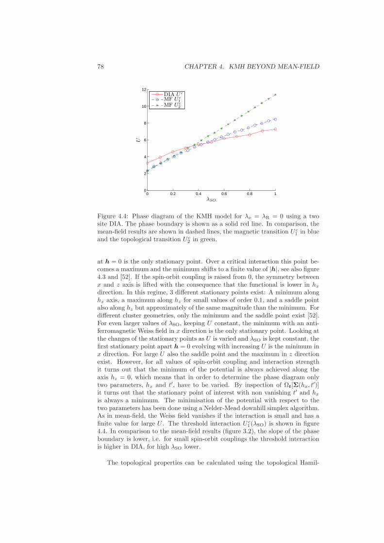
78 CHAPTER 4. KMH BEYOND MEAN-FIELD
0 0.2 0.4 0.6 0.8 10
2
4
6
8
10
12
λSO
U
DIA U c
MF U c1
MF U c2
Figure 4.4: Phase diagram of the KMH model for λν = λR = 0 using a twosite DIA. The phase boundary is shown as a solid red line. In comparison, themean-field results are shown in dashed lines, the magnetic transition U c
1 in blueand the topological transition U c
2 in green.
at h = 0 is the only stationary point. Over a critical interaction this point be-comes a maximum and the minimum shifts to a finite value of |h|, see also figure4.3 and [52]. If the spin-orbit coupling is raised from 0, the symmetry betweenx and z axis is lifted with the consequence that the functional is lower in hxdirection. In this regime, 3 different stationary points exist: A minimum alonghx axis, a maximum along hz for small values of order 0.1, and a saddle pointalso along hz but approximately of the same magnitude than the minimum. Fordifferent cluster geometries, only the minimum and the saddle point exist [52].For even larger values of λSO, keeping U constant, the minimum with an anti-ferromagnetic Weiss field in x direction is the only stationary point. Looking atthe changes of the stationary points as U is varied and λSO is kept constant, thefirst stationary point apart h = 0 evolving with increasing U is the minimum inx direction. For large U also the saddle point and the maximum in z directionexist. However, for all values of spin-orbit coupling and interaction strengthit turns out that the minimum of the potential is always achieved along theaxis hz = 0, which means that in order to determine the phase diagram onlytwo parameters, hx and t′, have to be varied. By inspection of Ωt[Σ(hx, t
′)]it turns out that the stationary point of interest with non vanishing t′ and hxis always a minimum. The minimisation of the potential with respect to thetwo parameters has been done using a Nelder-Mead downhill simplex algorithm.As in mean-field, the Weiss field vanishes if the interaction is small and has afinite value for large U . The threshold interaction U c
1 (λSO) is shown in figure4.4. In comparison to the mean-field results (figure 3.2), the slope of the phaseboundary is lower, i.e. for small spin-orbit couplings the threshold interactionis higher in DIA, for high λSO lower.
The topological properties can be calculated using the topological Hamil-
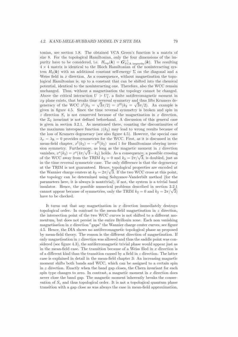
4.2. KANE-MELE-HUBBARD MODEL IN 2 SITE DIA 79
tonian, see section 1.8. The obtained VCA Green’s function is a matrix ofsize 8. For the topological Hamiltonian, only the four dimensions of the im-purity have to be considered, i.e. Htop(k) = G−1
VCA impurity(k). The resulting4 × 4 matrix is identical to the Bloch Hamiltonian of the noninteracting sys-tem H0(k) with an additional constant self-energy Σ on the diagonal and aWeiss field in x direction. As a consequence, without magnetisation the topo-logical Hamiltonian is, up to a constant that can be shifted into the chemicalpotential, identical to the noninteracting one. Therefore, also the WCC remainunchanged. Thus, without a magnetisation the topology cannot be changed.Above the critical interaction U > U c
1 , a finite antiferromagnetic moment inxy plane exists, that breaks time reversal symmetry and thus lifts Kramers de-generacy of the WCC xI(k2 =
√3π/2) = xII(k2 =
√3π/2). An example is
given in figure 4.5. Since the time reversal symmetry is broken and spin inz direction Sz is not conserved because of the magnetisation in x direction,the Z2 invariant is not defined beforehand. A discussion of this general caseis given in section 3.2.1. As mentioned there, counting the discontinuities ofthe maximum interspace function z(k2) may lead to wrong results because ofthe loss of Kramers degeneracy (see also figure 4.5). However, the special caseλν = λR = 0 provides symmetries for the WCC. First, as it is discussed in themean-field chapter, xI(k2) = −xII(k2) mod 1 for Hamiltonians obeying inver-sion symmetry. Furthermore, as long as the magnetic moment in z directionvanishes, xs(k2) = xs(4π/
√3− k2) holds. As a consequence, a possible crossing
of the WCC away from the TRIM k2 = 0 and k2 = 2π/√3, is doubled, just as
in the time reversal symmetric case. The only difference is that the degeneracyat the TRIM is not guaranteed. Hence, topological properties are encoded atthe Wannier charge centers at k2 = 2π/
√3. If the two WCC cross at this point,
the topology can be determined using Soluyanov-Vanderbilt method (for theparameters here, it is always is nontrivial), if not, the system is a trivial bandinsulator. Hence, the possible numerical problems described in section 3.2.1cannot appear because of symmetries, only the TRIM k2 = 0 and k2 = 2π/
√3)
have to be checked.
It turns out that any magnetisation in x direction immediately destroystopological order. In contrast to the mean-field magnetisation in z direction,the intersection point of the two WCC curves is not shifted to a different mo-mentum, but does not persist in the entire Brillouin zone. Each non vanishingmagnetisation in x direction ”gaps” the Wannier charge center curves, see figure4.5. Hence, the DIA shows no antiferromagnetic topological phase as proposedby mean-field theory. The reason is the different direction of magnetisation. Ifonly magnetisation in z direction was allowed and thus the saddle point was con-sidered (see figure 4.3), the antiferromagnetic trivial phase would appear just asin the mean-field case. The transition because of a Weiss filed in x direction isof a different kind than the transition caused by a field in z direction. The lattercase is explained in detail in the mean-field chapter 3: An increasing magneticmoment shifts both bands and WCC, which can be assigned to a certain spinin z direction. Exactly when the band gap closes, the Chern invariant for eachspin type changes to zero. In contrast, a magnetic moment in x direction doesnever close the band gap. The magnetic moment inherently breaks the conser-vation of Sz and thus topological order. It is not a topological quantum phasetransition with a gap close as was always the case in mean-field approximation,
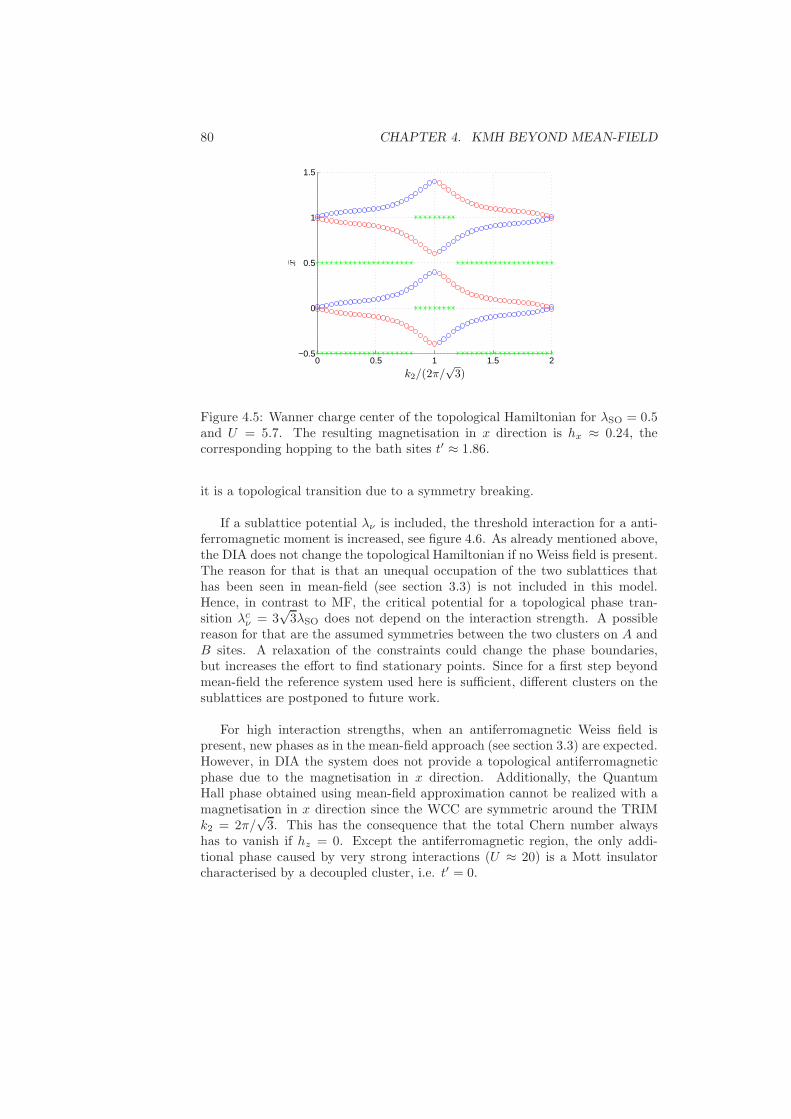
80 CHAPTER 4. KMH BEYOND MEAN-FIELD
0 0.5 1 1.5 2−0.5
0
0.5
1
1.5
x
k2/(2π/√
3)
Figure 4.5: Wanner charge center of the topological Hamiltonian for λSO = 0.5and U = 5.7. The resulting magnetisation in x direction is hx ≈ 0.24, thecorresponding hopping to the bath sites t′ ≈ 1.86.
it is a topological transition due to a symmetry breaking.
If a sublattice potential λν is included, the threshold interaction for a anti-ferromagnetic moment is increased, see figure 4.6. As already mentioned above,the DIA does not change the topological Hamiltonian if no Weiss field is present.The reason for that is that an unequal occupation of the two sublattices thathas been seen in mean-field (see section 3.3) is not included in this model.Hence, in contrast to MF, the critical potential for a topological phase tran-sition λcν = 3
√3λSO does not depend on the interaction strength. A possible
reason for that are the assumed symmetries between the two clusters on A andB sites. A relaxation of the constraints could change the phase boundaries,but increases the effort to find stationary points. Since for a first step beyondmean-field the reference system used here is sufficient, different clusters on thesublattices are postponed to future work.
For high interaction strengths, when an antiferromagnetic Weiss field ispresent, new phases as in the mean-field approach (see section 3.3) are expected.However, in DIA the system does not provide a topological antiferromagneticphase due to the magnetisation in x direction. Additionally, the QuantumHall phase obtained using mean-field approximation cannot be realized with amagnetisation in x direction since the WCC are symmetric around the TRIMk2 = 2π/
√3. This has the consequence that the total Chern number always
has to vanish if hz = 0. Except the antiferromagnetic region, the only addi-tional phase caused by very strong interactions (U ≈ 20) is a Mott insulatorcharacterised by a decoupled cluster, i.e. t′ = 0.
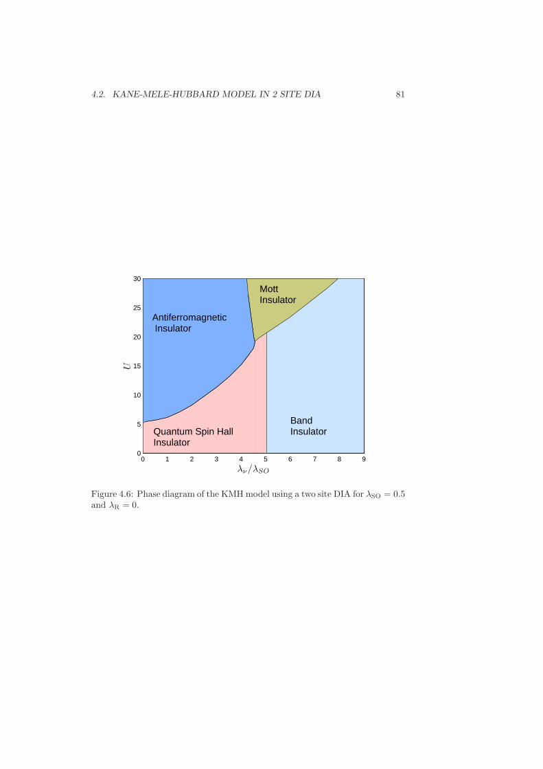
4.2. KANE-MELE-HUBBARD MODEL IN 2 SITE DIA 81
0 1 2 3 4 5 6 7 8 90
5
10
15
20
25
30
λν/λSO
U
Quantum Spin HallInsulator
BandInsulator
Antiferromagnetic Insulator
MottInsulator
Figure 4.6: Phase diagram of the KMHmodel using a two site DIA for λSO = 0.5and λR = 0.

82 CHAPTER 4. KMH BEYOND MEAN-FIELD
Chapter 5
Conclusions and outlook
Calculating topological invariants for strongly correlated systems is an inter-esting and demanding task since the picture of a topological one-particle bandstructure is not compatible with the many-body framework enforced by in-teractions. In this thesis, the Kane-Mele-Hubbard model was investigated tounderstand the influence of an interaction on a topological insulator. First,the noninteracting Kane-Mele model was analyzed in order to get a clear pic-ture of topological invariants in general and how they are affected by certainparameters. An introduction in topological invariants was given in chapter 1,resulting in the statement that the topological information is encoded in Wan-nier charge centers (WCC) which was highlighted by Soluyanov and Vanderbilt.This framework was used to explain the definition of the Z2 invariant given byFu and Kane, which is suitable for time-reversal symmetric systems. Further-more, another definition via the spin Chern number is given, which can only beused if the spin in z direction is conserved.
In chapter 2, the methods described above were applied to the noninteractingKane-Mele model. It was analyzed how spin-orbit coupling, sublattice potentialand Rashba coupling affect both band structure and WCC. Furthermore, thephase diagram valid for small spin-orbit couplings published by Kane and Melewas reproduced and expanded to large λSO. Finally, the results were comparedto the existence of edge states at a zigzag ribbon to check the bulk-boundarycorrespondence, which showed perfect agreement.
In order to introduce an interacting term, the Kane-Mele-Hubbard (KMH)Hamiltonian was considered in mean-field approximation. This simple theoryhas been chosen in order keep the WCC framework, which is based on the ex-istence Bloch states. In chapter 3, the phase diagram was analyzed in detail.It turned out that if the interaction U is large, an antiferromagnetic momentthat breaks time-reversal symmetry appears. It is important to mention thatthe topological spin order persists even when the magnetic moment is finite.The topological order is destroyed if the magnetic order exceeds a critical value.Furthermore, an on-site potential λν and a Rashba coupling λR were included,which causes additional phases. The spin ordering on the sublattices and theenergetic difference due to λν allow different absolute values of the two spinChern numbers. Hence, for a certain parameter set, a anomalous Hall phase is
83
84 CHAPTER 5. CONCLUSIONS AND OUTLOOK
possible. The chapter was concluded with a check of bulk-boundary correspon-dence in mean-field theory, which showed again perfect agreement. However, iftime-reversal symmetry and spin symmetry are broken simultaneously, the edgestates are gapped.
In the last chapter 4, a two-site Dynamical Impurity Approximation (DIA)was used to check the existence of various phases in a first step beyond mean-field. So-called topological Hamiltonians, that had been already introduced atthe end of chapter 1, were used in order to allow the calculation of WCC. Itturned out that the magnetic moment aligns in x direction, as already pub-lished by several other groups using different clusters or methods. In the simplemean-field approximation of chapter 3, a magnetisation in z direction had beeninherently assumed. The direction of magnetisation had great impact on thetopological order, since other symmetries are imposed on the WCC. WithinDIA, an antiferromagnetic quantum spin Hall state, which has been found inmean-field approximation, is not possible. Thus, one can conclude that thecorrect determination of the easy axis of a magnetic moment is of certain im-portance in order to determine the topology correctly.
The two-site DIA is a very simple model to test topology beyond mean-field.A further step would be to increase the cluster size in order to check the influenceof a nonlocal self-energy. This increases of course the effort to calculate thetopological Hamiltonian. A simpler addition to the work presented here wouldbe a mean-field approximation where the x axis is the reference direction. Thiscould possibly reproduce the DIA results qualitatively on a Hartree level. Thefinal goal is of course to use different models closer to real systems to predictstrongly correlated materials with nontrivial topology.
Appendix A
Kane-Mele Bloch
Hamiltonians
A.1 Bulk
In this appendix, matrix representation (2.20) is derived by writing the Kane-Mele Hamiltonian
HKM =− t∑
〈i,j〉c†i cj + iλSO
∑
〈〈i,j〉〉νijc
†iσ
zcj (A.1)
+ iλR∑
〈i,j〉c†i (σ × dij)zcj + λν
∑
i
ξic†icj
in the form HKM =∑
k؆
kH(k)Ψk, using the basis Ψ†
k= (a†
k↑, b†k↑, a
†k↓, b
†k↓),
where a†k↑ creates a spin up particle with momentum k on sublattice A. The
lattice geometry is defined in section 2.1. Lattice sites A are thus situated atR = na1 + ma2, lattice sites B at R + δ1. Hence, spinors c† ≡ (c†↑, c
†↓) are
transformed to momentum space by
c†R= a†
R=∑
k
eik·Ra†k
if i ∈ A, (A.2)
c†R
= b†R
=∑
k
eik·(R+δ1)b†k
if i ∈ B. (A.3)
The transformation of the sublattice potential term λν∑
i ξic†i cj is trivial since
it is diagonal. In the following, each of the remaining three terms is transformedseparately.
85
86 APPENDIX A. KANE-MELE BLOCH HAMILTONIANS
Tight-binding term:
−t∑
〈i,j〉c†i cj = −t
∑
〈i,j〉
(a†i bj + b†iaj
)= −t
∑
〈i,j〉a†ibj + h.c. (A.4)
∑
〈i,j〉a†i bj =
∑
R
3∑
l=1
a†RbR+δl
=∑
R
3∑
l=1
∑
kk′
ei(k·R−k′·(R+δl))a†
kbk′ (A.5)
=∑
k
3∑
l=1
e−ik·δla†kbk (A.6)
The sum over nearest-neighbors is combined to gk, which has been already usedin the dispersion relation of graphene (2.6). Simplifying the sum gives
gk/t ≡3∑
l=1
e−ik·δl = eiky√
3 + e−i
(
kx2+
ky
2√
3
)
+ e−i
(
−kx2+
ky
2√
3
)
(A.7)
=eiky√
3 + 2e−i
ky
2√
3 cos
(kx2
). (A.8)
The tight-binding term of the Kane-Mele model can thus be written as
−t∑
〈i,j〉c†i cj =
∑
k
gk a†kbk + h.c., (A.9)
with gk expressed above.
Spin-orbit coupling:
∑
〈〈i,j〉〉νijc
†iσ
zcj =∑
〈〈i,j〉〉νij
(c†i↑cj↑ − c†i↓cj↓
)(A.10)
=∑
〈〈i,j〉〉νij
(a†i↑aj↑ − a†i↓aj↓ + b†i↑bj↑ − b†i↓bj↓
)(A.11)
The 6 next-nearest-neighbor vectors are (see figure 2.1):
∆1,2 = ±a1 = ±1
2
(1√3
)∆3,4 = ±a2 = ±1
2
(−1√3
)(A.12)
∆5,6 = ±(a1 − a2) = ±(10
)(A.13)
Since the expression is similar for both sublattices, only sublattice A is treatedhere:
∑
〈〈i,j〉〉νij a
†iσajσ =
∑
R
6∑
l=1
ν∆la†RσaR+∆lσ (A.14)
=∑
R
6∑
l=1
∑
kk′
ν∆lei(k·R−k
′·(R+∆l))a†kσak′σ (A.15)
=∑
k
6∑
l=1
ν∆le−ik·∆la†
kσak′σ (A.16)
A.1. BULK 87
As for the tight-binding term, the sum over l is combined to γk. For the eval-uation of the sum, ∆l = −∆l+1 for l odd and ν∆ = −ν−∆ can be used, whichgives
γkiλSO
≡6∑
l=1
ν∆le−ik·∆l =
∑
l odd
ν∆l
(eik·∆l − e−ik·∆l
)(A.17)
=∑
l odd
ν∆l2i sin (k ·∆l) (A.18)
=i sin (kx)− i sin
(−kx
2+
√3ky2
)+ i sin
(−kx
2−
√3ky2
)(A.19)
=4i sin
(kx2
)cos
(√3ky2
)− 2i sin (kx) . (A.20)
For sublattice B, an overall minus sign appears since νA∆l= −νB∆l
, see figure2.4. Hence, the total spin-orbit term can be written as
iλSO∑
〈〈i,j〉〉νijc
†iσ
zcj =∑
k
gk
(a†k↑ak↑ − a†
k↓ak↓ − b†k↑bk↑ + b†
k↓bk↓). (A.21)
Rashba term:
∑
〈i,j〉c†i (σ × dij)zcj =
∑
〈i,j〉
(c†i↑c
†i↓
)(0 dy + idx
dy − idx 0
)(cj↑cj↓
)(A.22)
=∑
〈i,j〉
(dy + idx
)c†i↑cj↓ + h.c. (A.23)
Considering creation on sublattice A and annihilation on sublattice B, the re-lation
∑〈i,j〉 a
†i bj =
∑k
∑3l=1 e
−ik·δla†kbk has been already proven in equation
(A.6). In analogy, the relation
∑
〈i,j〉
(dy + idx
)a†i↑bj↓ =
∑
k
3∑
l=1
(δly + iδlx
)e−ik·δla†
k↑bk↓ (A.24)
holds. It has been used that the difference vector dij is equal to the nearest-neighbor vector δl. Inserting the nearest-neighbor vectors δ, the result for thesum over l is
ρkiλR
≡3∑
l=1
(δly + iδlx
)e−ik·δl (A.25)
=− e−iky3 +
(1
2+ i
√3
2
)ei(
kx2
+ky
2√
3
)
+
(1
2− i
√3
2
)ei(
− kx2+
ky
2√
3
)
(A.26)
=− e−i
ky√3 + e
iky
2√
3
(cos
(kx2
)−√3 sin
(kx2
)), (A.27)
which defines the term ρk. In the term which is related to a hopping from Ato B, the difference vector dij in equation (A.23) is not δl, but −δl. It is easy
88 APPENDIX A. KANE-MELE BLOCH HAMILTONIANS
to see that a transformation δ → −δ leads to ρk → −ρ−k. Hence, the Rashbaterm in momentum spaces takes the form
iλR∑
〈i,j〉c†i (σ × dij)zcj =
∑
k
(ρk a
†k↑bk↓ − ρ−k b
†k↑ak↓
)+ h.c. (A.28)
with ρk defined in equation A.27.
To sum up, after a Fourier transformation the three terms of the Kane-Meletake the form (A.9), (A.21) and (A.28). Writing these expressions and thesublattice potential term in matrix form as defined by equation 2.19, the BlochHamiltonian (2.20) is obtained. The explicit form of the coefficients gk, γk andρk given in the equations (2.21-2.23) is proven as can be seen from the relations(A.8), (A.20) and (A.27).
A.2 Zigzag ribbon
In the case of a bulk material, the transversal invariance in both x ans y directioncan be used to write the Hamiltonian in a block diagonal form (the Hamiltonianis diagonal in momentum k) so that only 4 degrees of freedom remain. A ribbonis translational invariant in only one direction. The unit cell of a zigzag ribbonis shown in figure 2.19. The size of the block diagonal parts for each kx is thenumber of sites in the unit cell times 2 (spin degree of freedom). In order tohave no dangling bonds, the number of sites of sublattice A within a unit cellhas to be equal to the number of sites of sublattice B and is in the following
denoted by N . We used, as in the bulk case, Ψ†kx
≡(a†kx↑, b
†kx↑, a
†kx↓, b
†kx↓
)as
a basis. Here, however, c†kxσ≡(c†kx1σ
, c†kx2σ, . . . c†kxNσ
)is a vector of length N .
Therefore, Ψ†kx
has dimension 4N . The Bloch Matrix H(kx) has the block form
H(kx) =
HA↑A↑ HA↑B↑ HA↑A↓ HA↑B↓H†
A↑B↑ HB↑B↑ HB↑A↓ HB↑B↓H†
A↑A↓ H†B↑A↓ HA↓A↓ HA↓B↓
H†A↑B↓ H†
B↑B↓ H†A↓A↓ HB↓B↓
(A.29)
where each block will be sparse (maximum tridiagonal for zigzag, pentadiagonalfor armchair ribbons) since only nearest and next-nearest-neighbor interactionsare considered. The analysis here is similar to the bulk case in section A.1.Therefore, only one hopping type within each term will be considered, for ex-ample, from A ↑ to B ↓ in the case of the Rashba coupling. The other hoppingscan be easily reconstructed using the results of the bulk in section A.1 by com-paring the block form of Bloch Hamiltonian (A.29) of the ribbon with the BlochHamiltonian (2.20) of the bulk. For example, HA↑A↑(kx) = HB↑B↑(kx) andHA↑B↓(kx) = −HB↑A↓(−kx). The only qualitative difference to the bulk case isthat the index m representing the y component remains since no translationalsymmetry in this direction is given. Therefore, m is the index or the row or thecolumn, respectively, of the block matrices in equation (A.29).
A.2. ZIGZAG RIBBON 89
Tight-binding term:
∑
〈i,j〉a†ibj =
∑
R
3∑
l=1
a†RbR+δl
(A.30)
=∑
nm
3∑
l=1
∑
kxk′x
ei(kxRnx−k′
x(Rnx+δlx))a†kxm
bkxm+dl (A.31)
=∑
ky
∑
m
3∑
l=1
e−ikxδlxa†kxm
bkxm+dl (A.32)
=∑
ky
∑
n
(e−iky
√3
2 a†kxmbkxm+1 + eiky
√3
2 a†kxmbkxm+1+ (A.33)
+ a†kxmbkxm−1
)(A.34)
=∑
ky
∑
m
2
(cos
(kx
√3
2
)a†kxm
bkxm+1 + a†kxmbkxm−1
)(A.35)
Spin-orbit coupling:
∑
〈〈i,j〉〉νij a
†iσajσ =
∑
R
6∑
l=1
ν∆la†RσaR+∆lσ (A.36)
=∑
nm
6∑
l=1
∑
kxk′x
ν∆lei(kxR
nx−k′
x(Rnx+∆l
x))a†kxmσakxm+Dlσ (A.37)
=∑
kx
∑
m
6∑
l=1
ν∆le−ikx∆
lxa†kxmσakxm+Dlσ (A.38)
As shown in figure 2.19, pairs of next-nearest-neighbor sites having the samey coordinate ∆y can be formed. The x component within a pair changes byfactor of −1, wherefore, as in equation (A.17), ν∆x,∆y
= −ν−∆x,∆ycan be used
to combine the exponential terms to sinuses. The final result is
∑
〈〈i,j〉〉νij a
†iσajσ =
∑
kx
∑
m
[− 2 sin
(kx
√3)a†kxmσakxmσ+
+ 2 sin
(kx
√3
2
)a†kxmσakxm+1σ+ (A.39)
+ 2 sin
(kx
√3
2
)a†kxmσakxm−1σ
].
Rashba coupling:
90 APPENDIX A. KANE-MELE BLOCH HAMILTONIANS
∑
〈i,j〉
(dy + idx
)a†i↑bj↓ =
=∑
m
∑
kx
3∑
l=1
(δly + iδlx
)e−ikxδlxa†kxm↑bkxm+dl↓ (A.40)
=1
2
∑
kx
∑
m
[(√3 + i)e−iky
√3
2 a†kxm↑bkxm+1↓+ (A.41)
+ (−√3 + i)eiky
√3
2 a†kxm↑bkxm+1↓ − 2ia†kxm↑bkxm−1↓]
= i∑
kx
∑
m
[(−√3 sin
(ky
3
2
)+ cos
(ky
3
2
))a†kxm↑bkxm+1↓− (A.42)
− 2a†kxm↑bkxm−1↓
]
With these results, the block matrices of equation (A.29) can be constructedeasily. For instance, HA↑A↑ is determined by equation (A.39) and has for N = 5the form
HA↑A↑(kx) =
α β 0 0 0β α β 0 00 β α β 00 0 β α β0 0 0 β α
(A.43)
with α = −2 sin(kx
√3)and β = 2 sin
(kx
√32
).
Bibliography
[1] M. V. Berry. Quantal phase factors accompanying adiabatic changes. Pro-ceedings of the Royal Society of London. A. Mathematical and PhysicalSciences, 392(1802):45–57, 1984.
[2] Yoichi Ando. Topological Insulator Materials. Journal of the PhysicalSociety of Japan, 82(10):102001, 2013.
[3] Katharina Durstberger. Geometric phases in quantum theory. Master’sthesis, Universitat Wien, 2002.
[4] Mikio Nakahara. Geometry, Topology and Physics. Institute of PhysicsPublishing, Dirac House, Temple Back, Bristol BS1 6BE, UK, 2 edition,2003.
[5] Mahito Kohmoto. Topological invariant and the quantization of the Hallconductance. Annals of Physics, 160(2):343 – 354, 1985.
[6] J. E. Avron, R. Seiler, and B. Simon. Homotopy and Quantization inCondensed Matter Physics. Phys. Rev. Lett., 51:51–53, Jul 1983.
[7] M. Z. Hasan and C. L. Kane. Colloquium: Topological insulators. Rev.Mod. Phys., 82:3045–3067, Nov 2010.
[8] Wu-Yi Hsiang and Dung-Hai Lee. Chern-Simons invariant in the Berryphase of a 2× 2 Hamiltonian. Phys. Rev. A, 64:052101, Oct 2001.
[9] K. v. Klitzing, G. Dorda, and M. Pepper. New method for high-accuracydetermination of the fine-structure constant based on quantized hall resis-tance. Phys. Rev. Lett., 45:494–497, Aug 1980.
[10] D. J. Thouless, M. Kohmoto, M. P. Nightingale, and M. den Nijs. QuantizedHall Conductance in a Two-Dimensional Periodic Potential. Phys. Rev.Lett., 49:405–408, Aug 1982.
[11] Wolfgang Nolting. Quantenmechanik - Grundlagen. Springer-Verlag,Berlin, Heidelberg, 7 edition, 2009.
[12] C. L. Kane and E. J. Mele. Quantum spin hall effect in graphene. Phys.Rev. Lett., 95:226801, Nov 2005.
[13] M. Hohenadler and F. F. Assaad. Correlation effects in two-dimensional topological insulators. Journal of Physics: Condensed Matter,25(14):143201, 2013.
91
92 BIBLIOGRAPHY
[14] D. N. Sheng, Leon Balents, and Ziqiang Wang. Phase diagram for quantumhall bilayers at ν = 1. Phys. Rev. Lett., 91:116802, Sep 2003.
[15] D. N. Sheng, Z. Y. Weng, L. Sheng, and F. D. M. Haldane. Quantum spin-hall effect and topologically invariant chern numbers. Phys. Rev. Lett.,97:036808, Jul 2006.
[16] Franz Schwabl. Quantenmechanik fur Fortgeschrittene (QMII). Springer-Verlag, Berlin, Heidelberg, 5 edition, 2008.
[17] Gregory H. Wannier. The structure of electronic excitation levels in insu-lating crystals. Phys. Rev., 52:191–197, Aug 1937.
[18] E.I. Blount. Formalisms of band theory. volume 13 of Solid State Physics,pages 305 – 373. Academic Press, 1962.
[19] Nicola Marzari and David Vanderbilt. Maximally localized generalizedWannier functions for composite energy bands. Phys. Rev. B, 56:12847–12865, Nov 1997.
[20] Liang Fu and C. L. Kane. Time reversal polarization and a Z2 adiabaticspin pump. Phys. Rev. B, 74:195312, Nov 2006.
[21] Jean Dalibard Jean-Louis Basdevant. Quantum Mechanics. Springer-Verlag, Berlin, Heidelberg, New York, 1 edition, 2005.
[22] Liang Fu and C. L. Kane. Topological insulators with inversion symmetry.Phys. Rev. B, 76:045302, Jul 2007.
[23] Alexey A. Soluyanov and David Vanderbilt. Computing topological invari-ants without inversion symmetry. Phys. Rev. B, 83:235401, Jun 2011.
[24] Qian Niu, D. J. Thouless, and Yong-Shi Wu. Quantized Hall conductanceas a topological invariant. Phys. Rev. B, 31:3372–3377, Mar 1985.
[25] V. Gurarie. Single-particle green’s functions and interacting topologicalinsulators. Phys. Rev. B, 83:085426, Feb 2011.
[26] Grigory E. Volovik. The Universe in a Helium Droplet. volume 117 ofInternational Series of Monographs on Physics, pages 305 – 373. OxfordUniversity Press, 2003.
[27] Andrew M. Essin and Victor Gurarie. Bulk-boundary correspondence oftopological insulators from their respective Green’s functions. Phys. Rev.B, 84:125132, Sep 2011.
[28] Zhong Wang, Xiao-Liang Qi, and Shou-Cheng Zhang. Topological invari-ants for interacting topological insulators with inversion symmetry. Phys.Rev. B, 85:165126, Apr 2012.
[29] Zhong Wang and Shou-Cheng Zhang. Simplified topological invariants forinteracting insulators. Phys. Rev. X, 2:031008, Aug 2012.
[30] Zhong Wang and Binghai Yan. Topological hamiltonian as an exacttool for topological invariants. Journal of Physics: Condensed Matter,25(15):155601, 2013.
BIBLIOGRAPHY 93
[31] R. Jackiw and C. Rebbi. Solitons with fermion number 12 . Phys. Rev. D,
13:3398–3409, Jun 1976.
[32] W. P. Su, J. R. Schrieffer, and A. J. Heeger. Solitons in polyacetylene.Phys. Rev. Lett., 42:1698–1701, Jun 1979.
[33] B. I. Halperin. Quantized hall conductance, current-carrying edge states,and the existence of extended states in a two-dimensional disordered po-tential. Phys. Rev. B, 25:2185–2190, Feb 1982.
[34] R. B. Laughlin. Quantized hall conductivity in two dimensions. Phys. Rev.B, 23:5632–5633, May 1981.
[35] Robert B. Laughlin. Nobel Lecture: Fractional Quantization.http://www.nobelprize.org/nobel_prizes/physics/laureates/
1998/laughlin-lecture.html, December 1998. [Online; Nobelprize.org.Nobel Media AB 2014. Web. 20 Feb 2015. ].
[36] Schulz-Baldes. Persistence of spin edge currents in disordered quantumspin Hall system. Commun. Math. Phys., 324:589–600, 2013.
[37] M. Porta G. M. Graf. Bulk-edge correspondence for two-dimensional topo-logical insulators . Commun. Math. Phys., 324:851–895, 2013.
[38] K. S. Novoselov, A. K. Geim, S. V. Morozov, D. Jiang, Y. Zhang, S. V.Dubonos, I. V. Grigorieva, and A. A. Firsov. Electric field effect in atomi-cally thin carbon films. Science, 306(5696):666–669, 2004.
[39] D. C. Elias, R. R. Nair, T. M. G. Mohiuddin, S. V. Morozov, P. Blake,M. P. Halsall, A. C. Ferrari, D. W. Boukhvalov, M. I. Katsnelson, A. K.Geim, and K. S. Novoselov. Control of graphene’s properties by reversiblehydrogenation: Evidence for graphane. Science, 323(5914):610–613, 2009.
[40] P. R. Wallace. The Band Theory of Graphite. Phys. Rev., 71:622–634, May1947.
[41] A. H. Castro Neto, F. Guinea, N. M. R. Peres, K. S. Novoselov, and A. K.Geim. The electronic properties of graphene. Rev. Mod. Phys., 81:109–162,Jan 2009.
[42] F. D. M. Haldane. Model for a quantum hall effect without landau levels:Condensed-matter realization of the ”parity anomaly”. Phys. Rev. Lett.,61:2015–2018, Oct 1988.
[43] Shuichi Murakami. Quantum spin hall phases. Progress of TheoreticalPhysics Supplement, 176:279–301, 2008.
[44] C. L. Kane and E. J. Mele. Quantum spin hall effect in graphene. Phys.Rev. Lett., 95:226801, Nov 2005.
[45] Jean-Christophe Charlier, Xavier Blase, and Stephan Roche. Electronicand transport properties of nanotubes. Rev. Mod. Phys., 79:677–732, May2007.
94 BIBLIOGRAPHY
[46] J. Hubbard. Electron correlations in narrow energy bands. Proceedings ofthe Royal Society of London A: Mathematical, Physical and EngineeringSciences, 276(1365):238–257, 1963.
[47] Wolfgang Nolting. Viel-Teilchen-Theorie. Springer-Verlag, Berlin, Heidel-berg, New York, 6 edition, 2009.
[48] Stephan Rachel and Karyn Le Hur. Topological insulators and mott physicsfrom the hubbard interaction. Phys. Rev. B, 82:075106, Aug 2010.
[49] Dong Zheng, Guang-Ming Zhang, and Congjun Wu. Particle-hole symme-try and interaction effects in the kane-mele-hubbard model. Phys. Rev. B,84:205121, Nov 2011.
[50] Wei Wu, Stephan Rachel, Wu-Ming Liu, and Karyn Le Hur. Quantumspin hall insulators with interactions and lattice anisotropy. Phys. Rev. B,85:205102, May 2012.
[51] Jan Carl Budich, Ronny Thomale, Gang Li, Manuel Laubach, and Shou-Cheng Zhang. Fluctuation-induced topological quantum phase transi-tions in quantum spin-hall and anomalous-hall insulators. Phys. Rev. B,86:201407, Nov 2012.
[52] Manuel Laubach, Johannes Reuther, Ronny Thomale, and Stephan Rachel.Rashba spin-orbit coupling in the Kane-Mele-Hubbard model. Phys. Rev.B, 90:165136, Oct 2014.
[53] Potthoff, M. Self-energy-functional approach to systems of correlated elec-trons. Eur. Phys. J. B, 32(4):429–436, 2003.
[54] J. M. Luttinger and J. C. Ward. Ground-state energy of a many-fermionsystem. ii. Phys. Rev., 118:1417–1427, Jun 1960.
[55] M. Potthoff. Self-energy-functional approach: Analytical results and themott-hubbard transition. The European Physical Journal B - CondensedMatter and Complex Systems, 36(3):335–348, 2003.
[56] M. Potthoff, M. Aichhorn, and C. Dahnken. Variational cluster approach tocorrelated electron systems in low dimensions. Phys. Rev. Lett., 91:206402,Nov 2003.
[57] M. Aichhorn, E. Arrigoni, M. Potthoff, and W. Hanke. Variational clusterapproach to the hubbard model: Phase-separation tendency and finite-sizeeffects. Phys. Rev. B, 74:235117, Dec 2006.
[58] David Senechal. An introduction to quantum cluster methods.arXiv:0806.2690v2 [cond-mat.str-el], November 2010.
[59] Marc G. Zacher, Robert Eder, Enrico Arrigoni, and Werner Hanke. Evolu-tion of the stripe phase as a function of doping from a theoretical analysisof angle-resolved photoemission data. Phys. Rev. B, 65:045109, Jan 2002.
[60] Christopher N. Varney, Kai Sun, Marcos Rigol, and Victor Galitski. Topo-logical phase transitions for interacting finite systems. Phys. Rev. B,84:241105, Dec 2011.