Embed Size (px)
Citation preview
Lesson 1
Walrasian Equilibrium in a pure Exchange Economy.
General Model
Chapter 16 2©2005 Pearson Education, Inc.
General Model: Economy with n agents and k goods.
Goods. Concept of good: good or service completely specified phisically, spacially and timely. Assumption 1 : There is a finite number k of goods. Assumption 2 : Goods can be consumed in any non-negative real number.Goods are perfectly divisible The space of goods is kR+
Chapter 16 3©2005 Pearson Education, Inc.
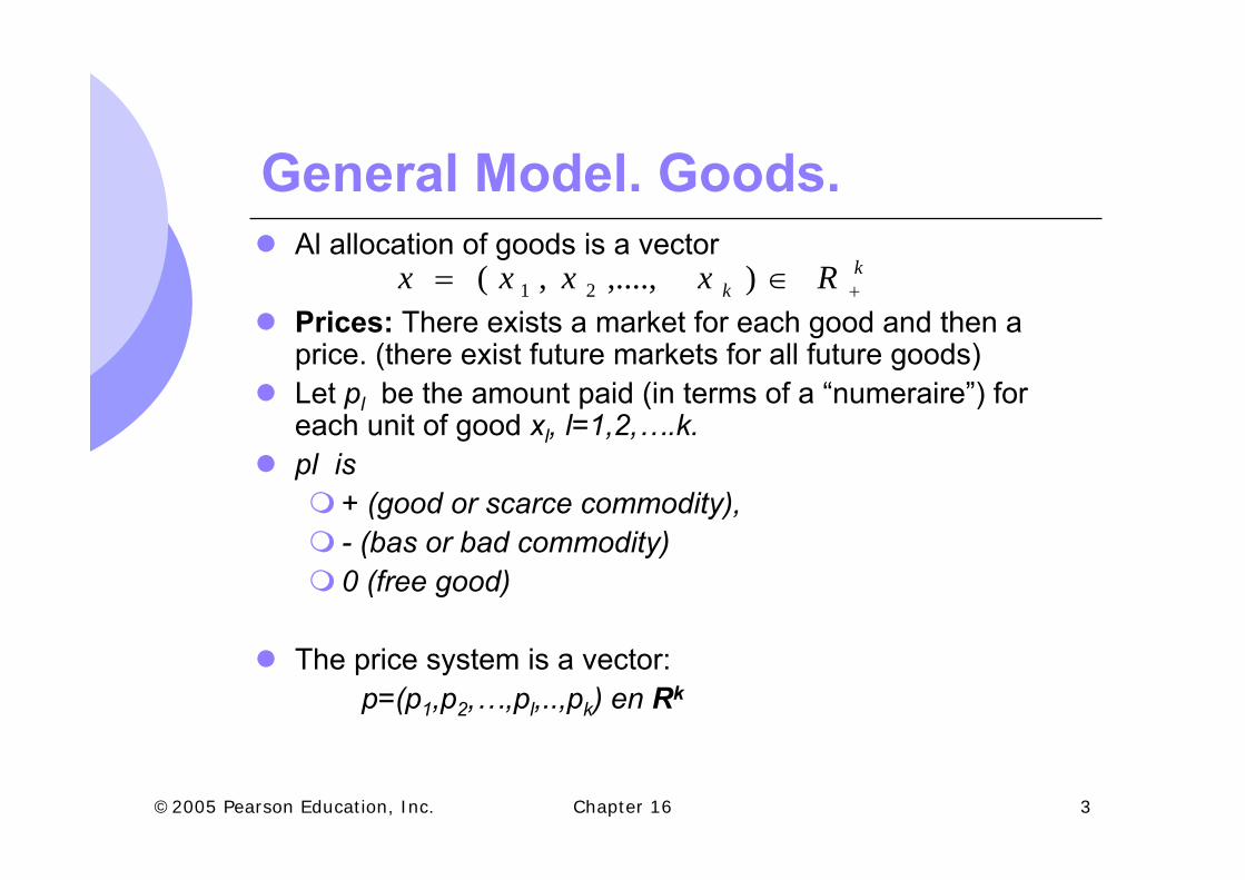
General Model. Goods.Al allocation of goods is a vector
Prices: There exists a market for each good and then a price. (there exist future markets for all future goods)Let pl be the amount paid (in terms of a “numeraire”) for each unit of good xl, l=1,2,….k. pl is
+ (good or scarce commodity), - (bas or bad commodity) 0 (free good)
The price system is a vector: p=(p1,p2,…,pl,..,pk) en Rk
kk Rxxxx +∈= ),....,,( 21

Chapter 16 4©2005 Pearson Education, Inc.
General Model.
Barter EconomyThe economy works out without the help of the good money (or any other good as accounting measure)The model is of perfect information (or perfect forecast) The model is static. Steady state (the dynamic structure is not in the model).Agents choose “consumption plans for all their lives)
Chapter 16 5©2005 Pearson Education, Inc.
General Model. Agents.
Assumption 1. A finite number, n, of consumers.Consumer’s aim= To choose a consumption plan according to her choice-criterion and her survival (consumption set) and wealth constraints. Choice criterion: An economic decision maker always chooses her most preferred alternative from the set of available alternatives.Assumption 2 : consumers are price-takers.Description of an economic agent: Each consumer i defined by:
Her consumption set Xi
Her initial endowmentsHer preferences over baskets of goods.
kik
iii RwwwW +∈= ),....,,( 21
Chapter 16 6©2005 Pearson Education, Inc.
General Model. Agents. The consumption set: Example: Survival.Assumption C1:
Assumption C2: Xi is convex and closed(perfect divisibility)
ki RX +⊂
ki RX +=
kiik
iii RXxxxx +=∈= ),....,,( 21
Chapter 16 7©2005 Pearson Education, Inc.
General Model. Preferences: Binary relationship between bundles of goods.
f denotes strict preference:x f y means that x is strictly preferred (o is strictly better than) to y.∼ denotes indiference:x ∼ y means that x and y equally preferred (is exactly
as good as).
< denotes weak preference
x < y means that x is at least as preferred as (or is at least as good) as y.
Chapter 16 8©2005 Pearson Education, Inc.
Assumptions on preferences
Assumption 2. Reflexivity: x < x.Assumption 3. Transitivity: if x < y and y < z, then x < z.Assumption 1. Completeness: either x < y, or y < x, or both.
Pre-order in X. The indiference relationship partitions X in equivalence clases, which are disjoints and exhaustives =Indiference sets with at least one element (by reflexivity)
Chapter 16 9©2005 Pearson Education, Inc.
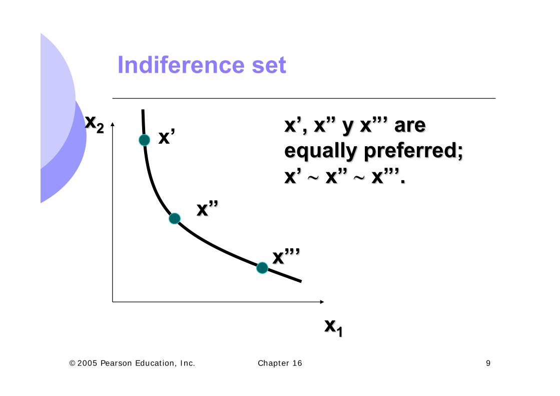
Indiference set
xx22
xx11
xx””
xx”’”’
xx’’, x, x”” y xy x”’”’ areareequally preferred;equally preferred;xx’’ ∼∼ xx”” ∼∼ xx”’”’..
x’
Chapter 16 10©2005 Pearson Education, Inc.
General Model. Utility function.Utility function: Rule associating a real number to each vector of
goods in X:U: X→R, such that
x f y ↔ u(x) >u(y) ; x ∼ y ↔ u(x) =u(y).
An isomorphism is need (an order preserving relationship betwensets) between X y R, in order that preferences are representedby an utility function.
Let I be the set of equivalence classes.
(I, f) is isomorphic to (Q, f), where Q is the set of rationalnumber, whenever set I is finite.
If I is not finite, and additional assumption is need to guaranteethat preferences are representable by utility functions.
Chapter 16 11©2005 Pearson Education, Inc.
General Model. PreferencesAssumption 4. Continuity. For all x and y εX, the sets {x: x < y } and {x: x - y} are closed.
Theorem: If < satisfies completeness, reflexivity, transitivityand continuty, then there exists an utility function U: X→Rrepresenting these preferences. U is continuos and satisfiesthat u(x)≥u(y) if and only if x < y.
U(.) is ordinal and uniquely represents < if all the positive transformations of U(.) are included.
If U(.) represents < and if f:R→R is a monotone increasingfunction, then f(u(x)) also represents < since f(u(x))≥f(u(y)) if and only if u(x)≥u(y).
Chapter 16 12©2005 Pearson Education, Inc.
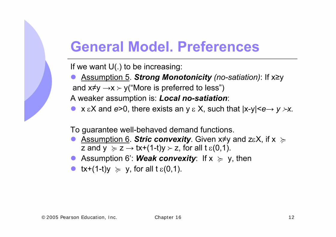
General Model. PreferencesIf we want U(.) to be increasing:
Assumption 5. Strong Monotonicity (no-satiation): If x≥yand x≠y →x f y(“More is preferred to less”)
A weaker assumption is: Local no-satiation:x εX and e>0, there exists an y ε X, such that |x-y|<e→ y fx.
To guarantee well-behaved demand functions.Assumption 6. Stric convexity. Given x≠y and zεX, if x <z and y < z → tx+(1-t)y f z, for all t ε(0,1). Assumption 6’: Weak convexity: If x < y, thentx+(1-t)y < y, for all t ε(0,1).
Chapter 16 13©2005 Pearson Education, Inc.
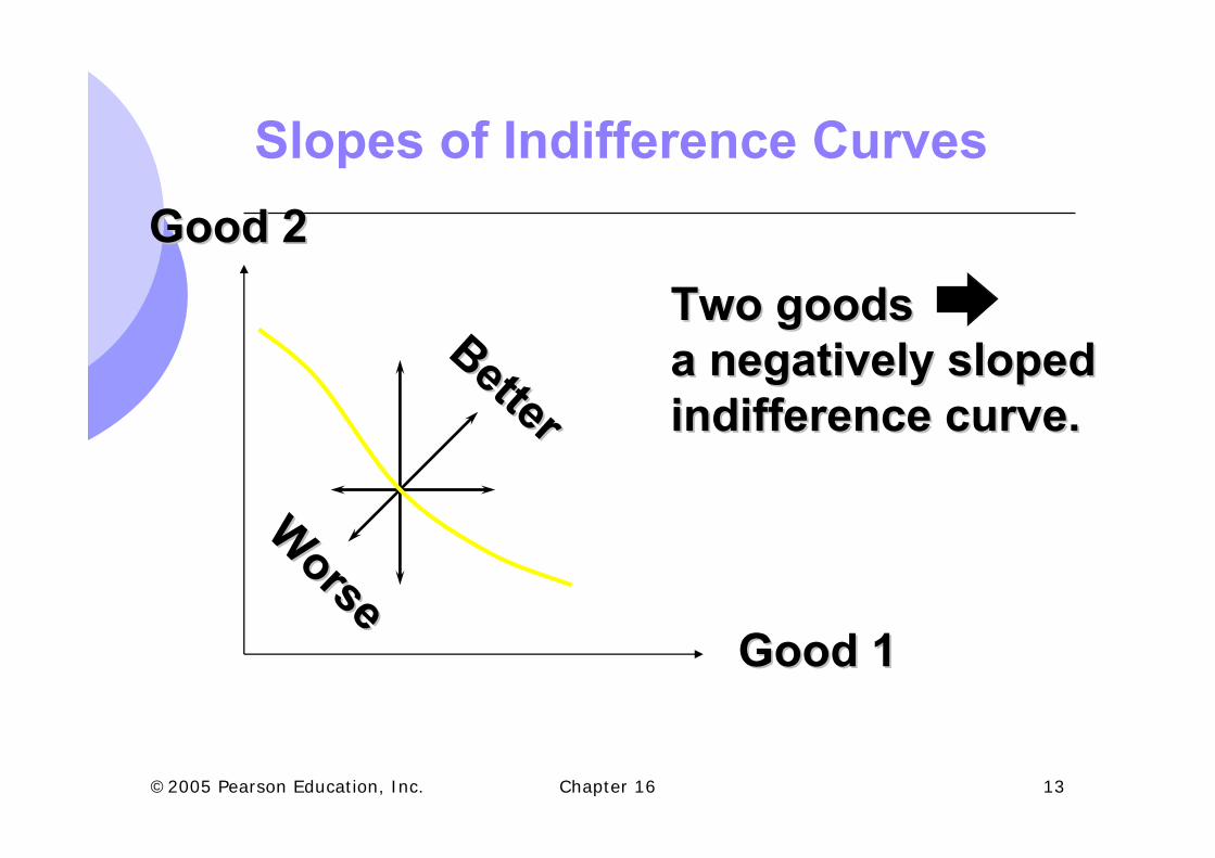
Slopes of Indifference Curves
BetterBetter
Worse
Worse
Good 2Good 2
Good 1Good 1
Two goodsTwo goodsa negatively sloped a negatively sloped indifference curve.indifference curve.
Chapter 16 14©2005 Pearson Education, Inc.
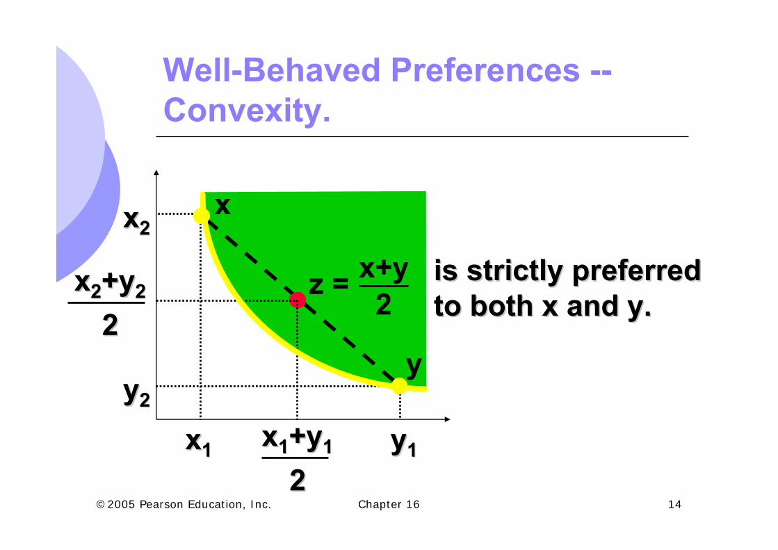
Well-Behaved Preferences --Convexity.
xx22
yy22
xx22+y+y22
22
xx11 yy11xx11+y+y11
22
x
y
z = x+y2
is strictly preferred is strictly preferred to both x and y.to both x and y.
Chapter 16 15©2005 Pearson Education, Inc.
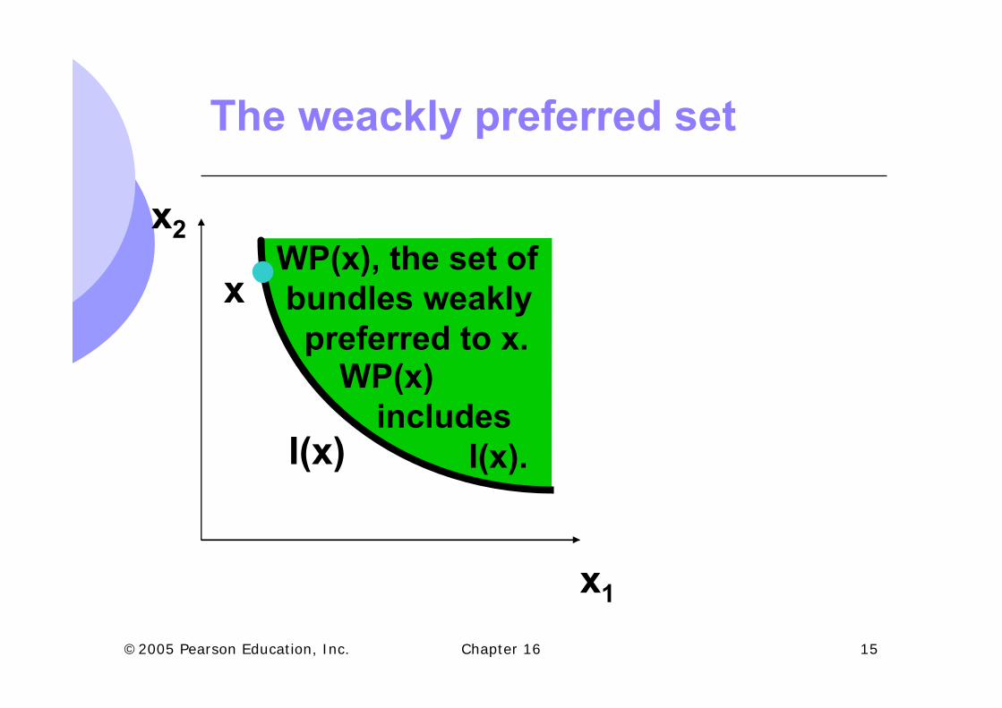
The weackly preferred set
x2
x1
WP(x), the set ofbundles weaklypreferred to x.
WP(x)includes
I(x).
x
I(x)
Chapter 16 16©2005 Pearson Education, Inc.
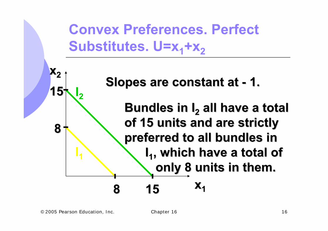
Convex Preferences. Perfect Substitutes. U=x1+x2
xx22
xx1188
88
1515
1515Slopes are constant at Slopes are constant at -- 1.1.
I2
I1
Bundles in IBundles in I22 all have a totalall have a totalof 15 units and are strictlyof 15 units and are strictlypreferred to all bundles inpreferred to all bundles in
II11, which have a total of, which have a total ofonly 8 units in them.only 8 units in them.
Chapter 16 17©2005 Pearson Education, Inc.
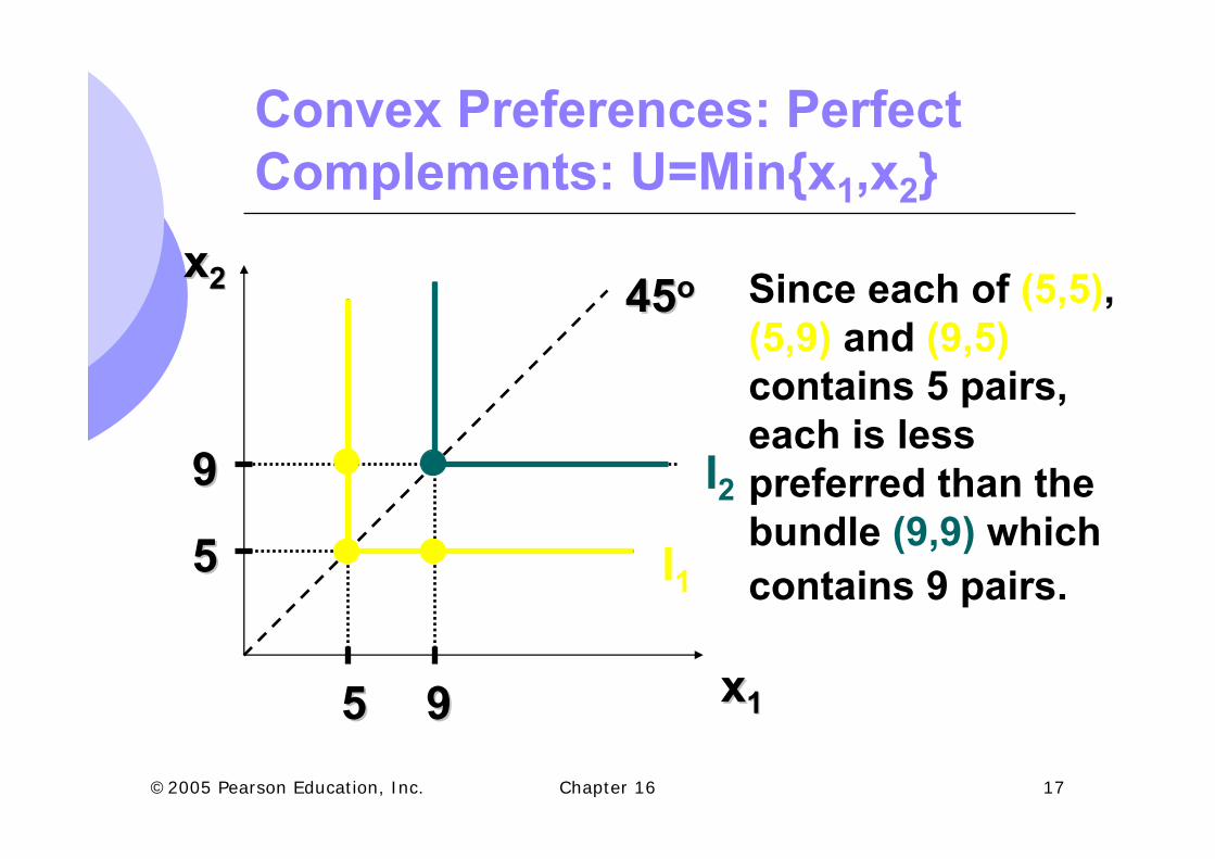
Convex Preferences: Perfect Complements: U=Min{x1,x2}
xx22
xx11
I2
I1
4545oo
55
99
55 99
Since each of (5,5), (5,9) and (9,5)contains 5 pairs, each is less preferred than the bundle (9,9) which contains 9 pairs.
Chapter 16 18©2005 Pearson Education, Inc.
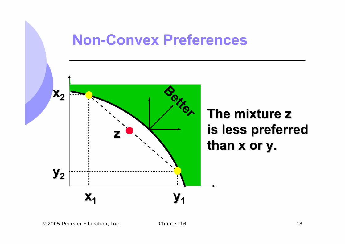
Non-Convex Preferences
xx22
yy22
xx11 yy11
zz
Better The mixture zThe mixture zis less preferredis less preferredthan x or y.than x or y.
Chapter 16 19©2005 Pearson Education, Inc.
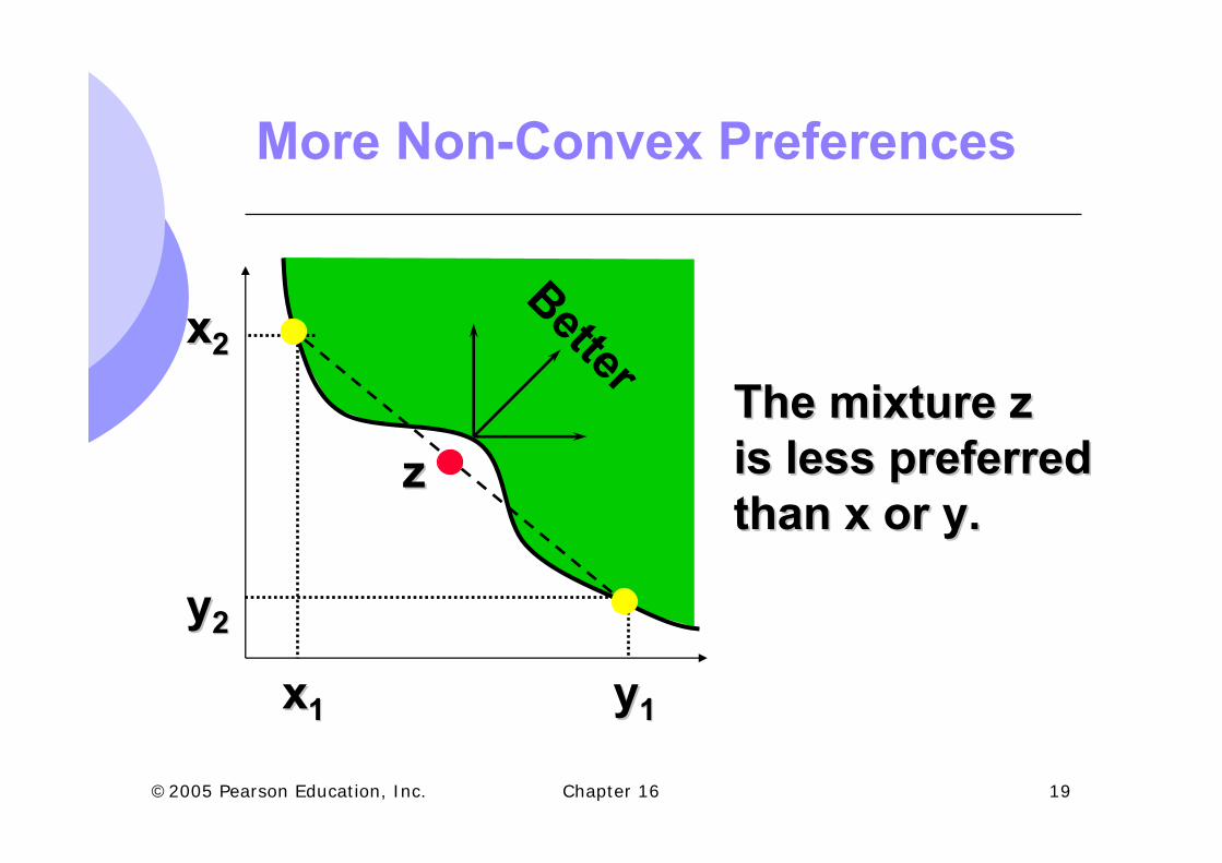
More Non-Convex Preferences
xx22
yy22
xx11 yy11
zz
Better
The mixture zThe mixture zis less preferredis less preferredthan x or y.than x or y.
Chapter 16 20©2005 Pearson Education, Inc.
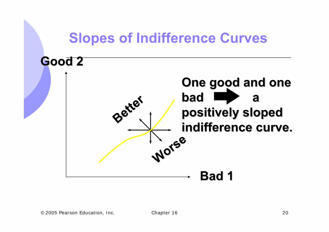
Slopes of Indifference Curves
Better
Better
WorseWorse
Good 2Good 2
Bad 1Bad 1
One good and oneOne good and onebad a bad a positively sloped positively sloped indifference curve.indifference curve.
Chapter 16 21©2005 Pearson Education, Inc.
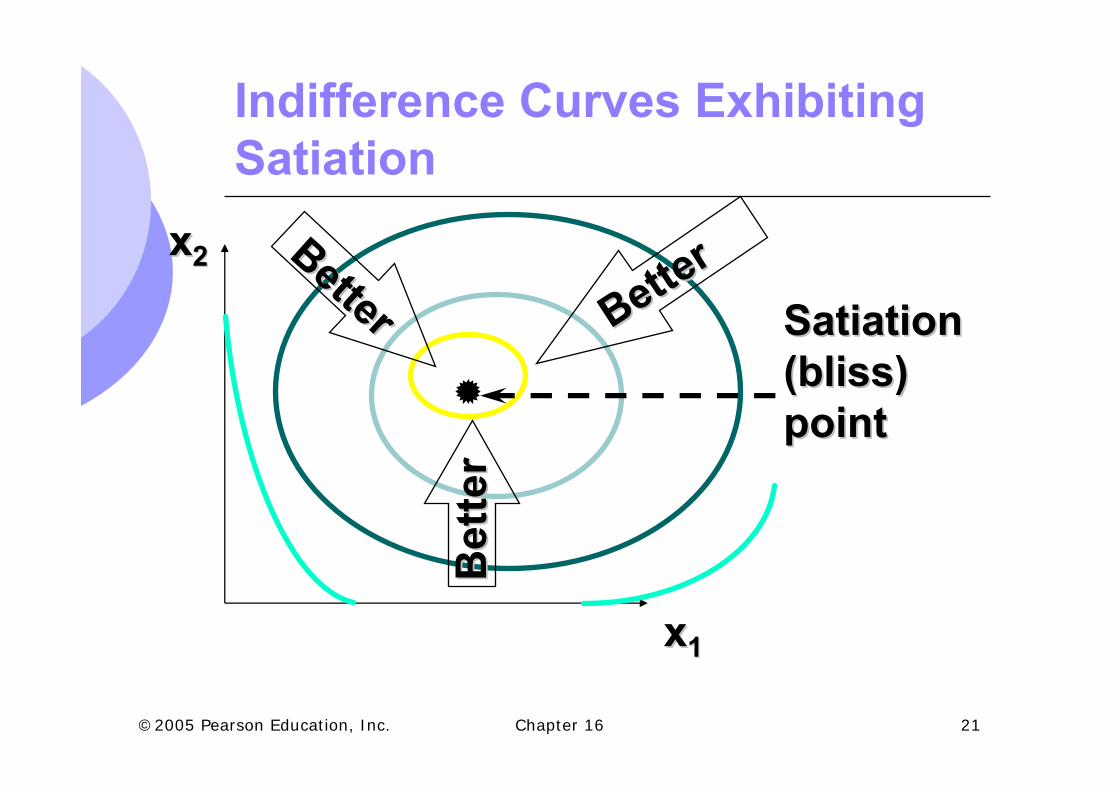
Indifference Curves Exhibiting Satiation
xx22
xx11
BetterBetterBetter
Better
Bet
ter
Bet
ter
SatiationSatiation(bliss)(bliss)pointpoint
Chapter 16 22©2005 Pearson Education, Inc.
Preferences and UtilityTheorem: If < satisfy the assumptions (1)-(6), then < can be represented by a utility functionU(.), which is continuos, increasing and strictlyquasi-concave.
Consumer i is characterized bya) Her consumption set: Xi
b) Her preferences < i → ui(.)c) Her initial endowments wi .
Allocation: x=(x1,x2,….,xn) a collection of nconsumption plans. Feasible allocation:
1 1
n ni i
i ix w
= =
=∑ ∑
Chapter 16 23©2005 Pearson Education, Inc.
Demand functions and aggregatedemand. Existence and characterization.
Question: Is there a price vector p such that: 1) eachconsumer i maximizes her ui(.) and 2) the n-consumption plans are compatible?
1. Demand functions (Existence)Weiertrass’ Theorem: Let f be a real continuous function definedin a compact set of an n-dimensional space, then f achieves itsextreme values (maximum and minimum) in some points of theset→Implies:
Let f: Rn→R be continuous and A⊂ Rn a compact set, then thereexits a vector x* solving:
Max f(x)subject to xε A
Chapter 16 24©2005 Pearson Education, Inc.
Demand functions.Existence
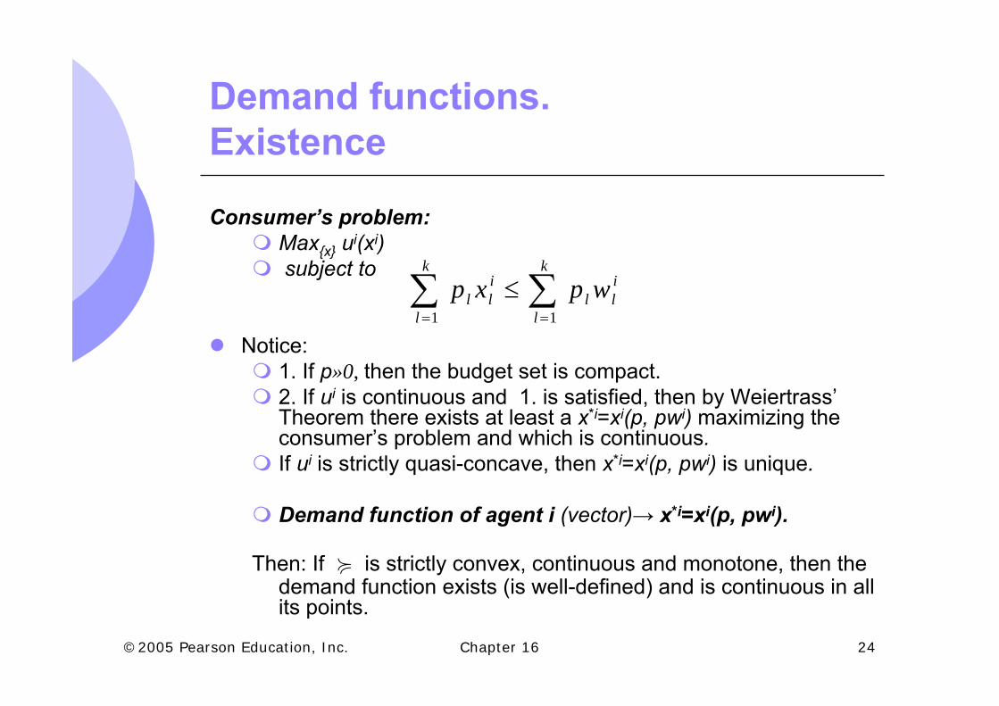
Consumer’s problem:Max{x} ui(xi)subject to
Notice:1. If p»0, then the budget set is compact.2. If ui is continuous and 1. is satisfied, then by Weiertrass’Theorem there exists at least a x*i=xi(p, pwi) maximizing the consumer’s problem and which is continuous. If ui is strictly quasi-concave, then x*i=xi(p, pwi) is unique.
Demand function of agent i (vector)→ x*i=xi(p, pwi).
Then: If < is strictly convex, continuous and monotone, then the demand function exists (is well-defined) and is continuous in all its points.
1 1
k ki i
l l l ll l
p x p w= =
≤∑ ∑
Chapter 16 25©2005 Pearson Education, Inc.
Demand functions.Characterization.
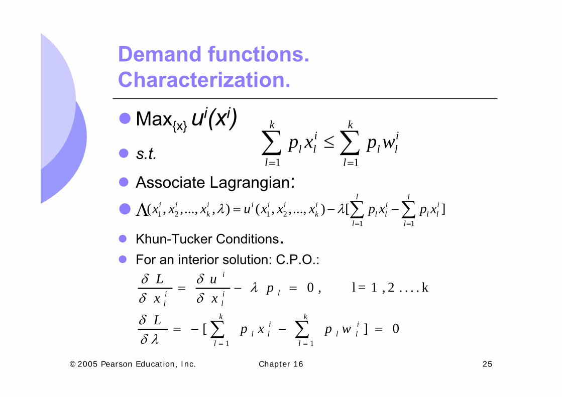
Max{x} ui(xi)s.t.
Associate Lagrangian:ΛKhun-Tucker Conditions.For an interior solution: C.P.O.:
1 1
k ki i
l l l ll l
p x p w= =
≤∑ ∑
1 2 1 21 1
( , ,..., , ) ( , ,..., ) [ ]l l
i i i i i i i i ik k l l l l
l l
x x x u x x x p x p xλ λ= =
= − −∑ ∑
1 1
0 , l = 1 , 2 . . . . k
[ ] 0
i
li il l
k ki i
l l l ll l
L u px xL p x p w
δ δ λδ δδδ λ = =
= − =
= − − =∑ ∑
Chapter 16 26©2005 Pearson Education, Inc.
Marshallian or ordinary demandfunctions. Net demand functions. Comparative Statics.
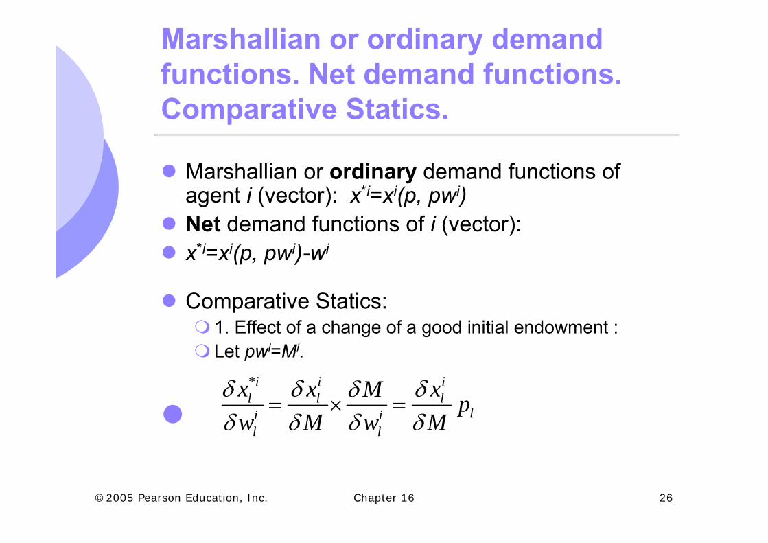
Marshallian or ordinary demand functions of agent i (vector): x*i=xi(p, pwi)Net demand functions of i (vector):x*i=xi(p, pwi)-wi
Comparative Statics:1. Effect of a change of a good initial endowment :Let pwi=Mi.
*i i il l l
li il l
x x xM pw M w M
δ δ δδδ δ δ δ
= × =
Chapter 16 27©2005 Pearson Education, Inc.
Comparative Statics. Slutsky’s equation.
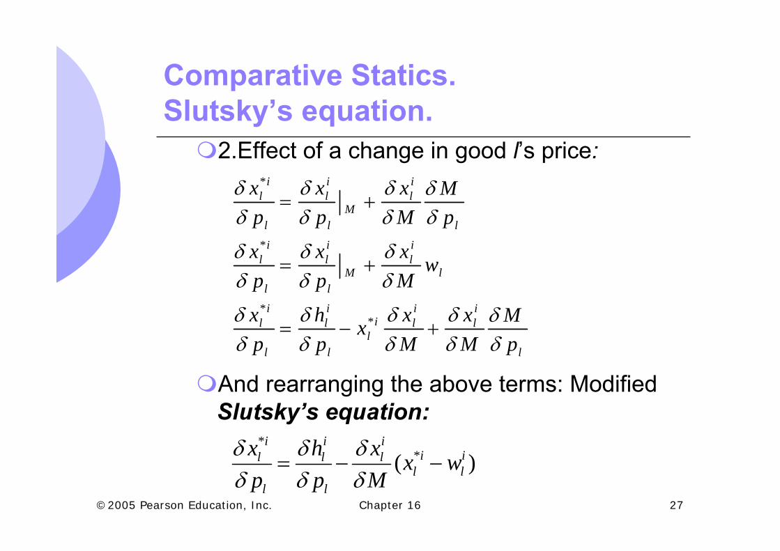
2.Effect of a change in good l’s price:
And rearranging the above terms: ModifiedSlutsky’s equation:
*
*
**
i i il l l
Ml l l
i i il l l
M ll l
i i i iil l l l
ll l l
x x x Mp p M p
x x x wp p M
x h x x Mxp p M M p
δ δ δ δδ δ δ δ
δ δ δδ δ δ
δ δ δ δ δδ δ δ δ δ
= +
= +
= − +
**( )
i i ii il l l
l ll l
x h x x wp p M
δ δ δδ δ δ
= − −
Chapter 16 28©2005 Pearson Education, Inc.
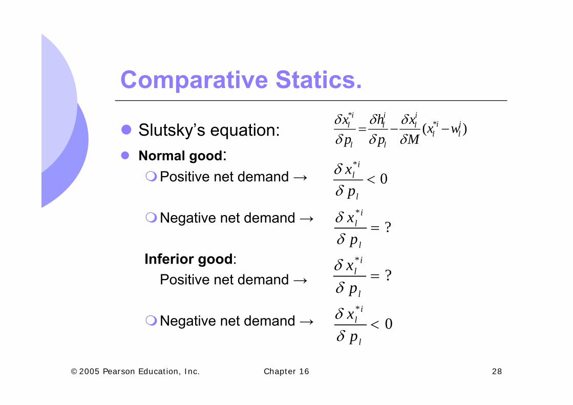
Comparative Statics.
Slutsky’s equation:Normal good:
Positive net demand →
Negative net demand →
Inferior good: Positive net demand →
Negative net demand →
**( )
i i ii il l l
l ll l
x h x x wp p M
δ δ δδ δ δ
= − −
*
0i
l
l
xp
δδ
<
*
?i
l
l
xp
δδ
=
*
?i
l
l
xp
δδ
=
*
0i
l
l
xp
δδ
<
Chapter 16 29©2005 Pearson Education, Inc.
Aggregate demand
Addition set: With the individualism hypotesis onpreferences→aggregate quantities=sum of individual quantities (there is not externalities)
x*i=xi(p, pwi) vector of i’s demand funtions. X(p)=∑i x*i= ∑i xi(p, pwi) , aggregate demand function of the Economy.
At each market l:xl*i =xl
i(p, pwi) is i’s demand function of good l, andXl(p)= ∑i xl
i(p, pwi) is the market aggregate demand function of good l.

Chapter 16 30©2005 Pearson Education, Inc.
Walrasian Equilibrium:
Let p=(p1,p2,…,pk) be a price vector.
Each agent i: Max{x} ui(xi) subjet to pxi=pwi
Solution: demand function of i: x*i=xi(p, pwi) Aggregate demand: X(p)=∑i x*i= ∑i xi(p, pwi) Aggregate supply: ∑i wi.
Is there a price vector p* such that∑i xi(p, pwi)= ∑i wi , and with free goods∑i xi(p, pwi)6 ∑i wi ?
Chapter 16 31©2005 Pearson Education, Inc.
Walrasian equilibrium:
Let z(p)=∑i xi(p, pwi)- ∑iwi be the excess demandfunction of the economy, and
Let zj (p)=∑i xji(p, pwi)- ∑iwj
i, be the excess demand function of good (market) j.
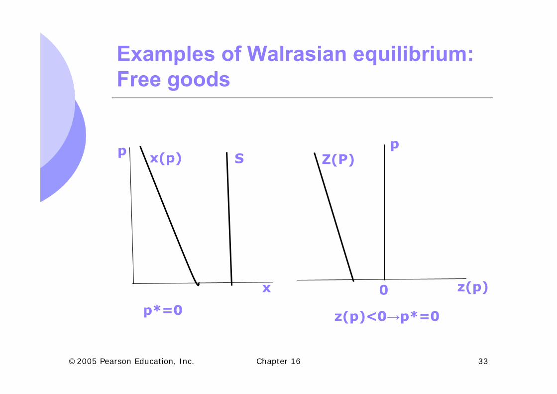
A price vector p* ≥0, is a walrasian equilibrium(or competitive equilibrium) if:zj (p*)=0, if j is scarce (pj
* >0)zj (p*)<0 if j is a free good (pj
* =0)
Chapter 16 32©2005 Pearson Education, Inc.
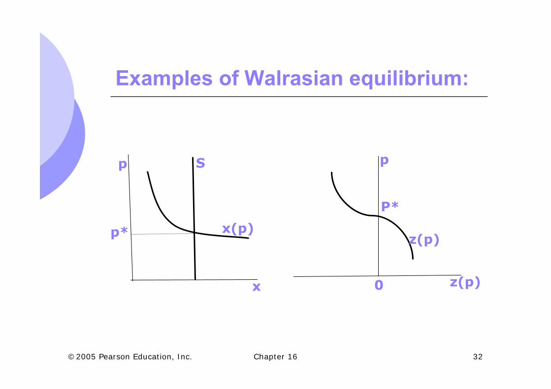
Examples of Walrasian equilibrium:
x
p p
z(p)0
p*
P*
x(p)
S
z(p)
Chapter 16 33©2005 Pearson Education, Inc.
Examples of Walrasian equilibrium: Free goods
x
p p
z(p)0
x(p) S
p*=0 z(p)<0→p*=0
Z(P)
Chapter 16 34©2005 Pearson Education, Inc.
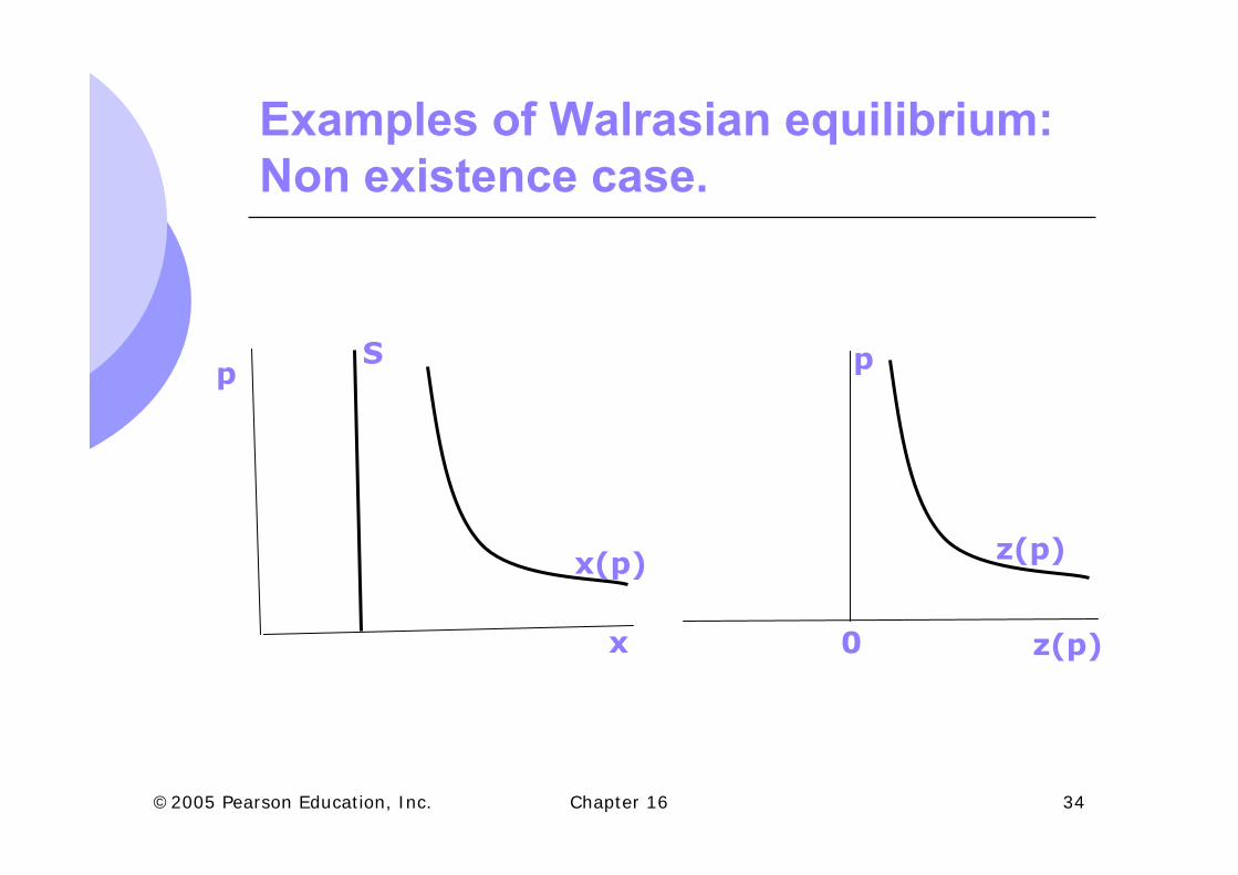
Examples of Walrasian equilibrium: Non existence case.
x
p p
z(p)0
x(p)
S
z(p)
Chapter 16 35©2005 Pearson Education, Inc.
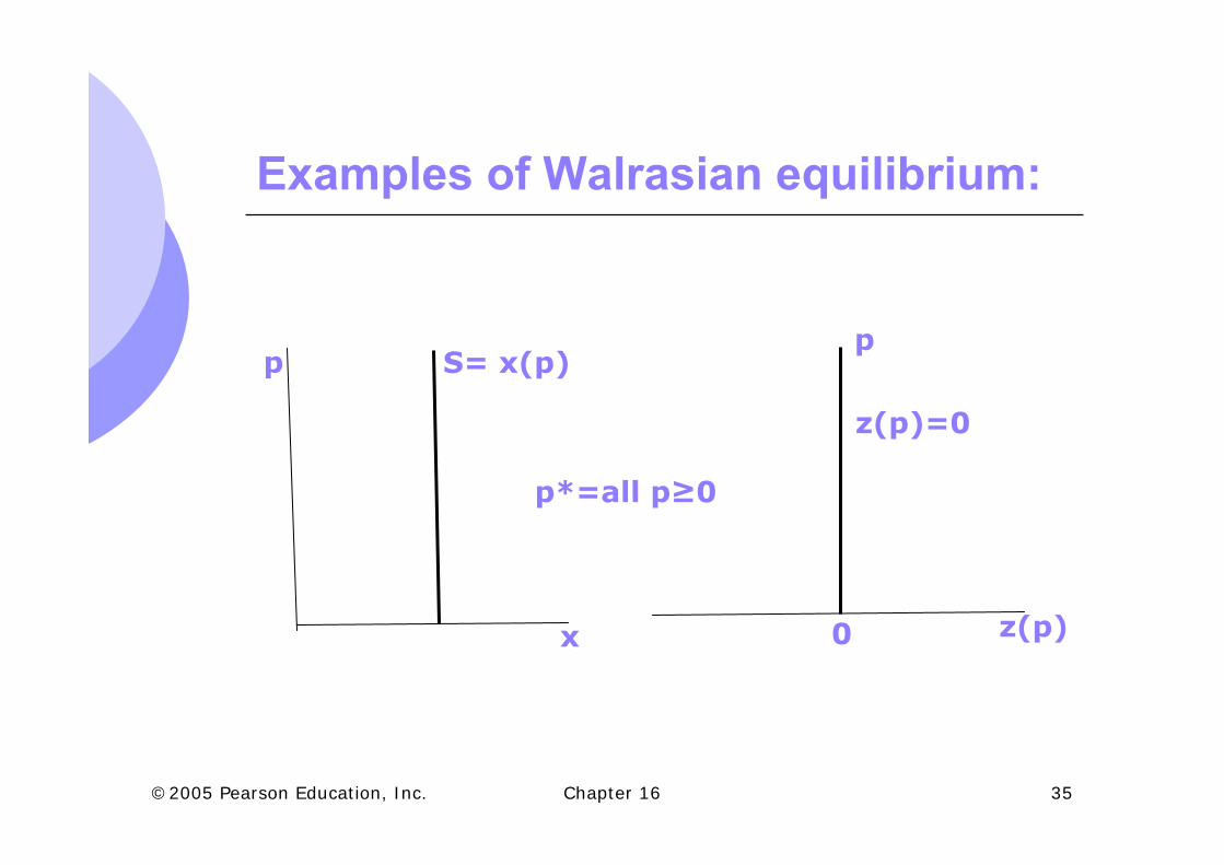
Examples of Walrasian equilibrium:
x
pp
z(p)0
p*=all p≥0
S= x(p)
z(p)=0
Chapter 16 36©2005 Pearson Education, Inc.
Walrasian equilibrium: Properties of theexcess demand function z(p).
Let us come back to our model: Is there a price vector p* such that allmarkets clear? First: properties of z(p). Notice:
1) The budget set of each agent i does not vary if all prices are multiplied by the same constant:→ the budget set is homogeneousof degree zero in prices. 2) By 1)→The demand function is homogeneous of degree zero in prices: xi(kp,kpwi)= xi(p,pwi).3) The sum of homogeneous functions of degree r is anotherhomogeneous function of degree r:→the aggregate demand functionis homogeneous of degree zero in prices: ∑i xi(p,pwi) ishomogeneous of degree zero n prices. 4) The excess demand function z(p)= ∑i xi(p,pwi)-∑iwi ishomogeneous of degree zero in prices. 5) By the assumptions on < (convexity) the demand function iscontinuous and since the sum of continuous functions iscontinuous→the aggregate demand function is continuous: z(p) is a continuous function.
Z(p) is a continuous and homogeneous function of degreezero in prices.
Chapter 16 37©2005 Pearson Education, Inc.
Walrasian equilibrium. Existence: Brower’s fixed point Theorem.
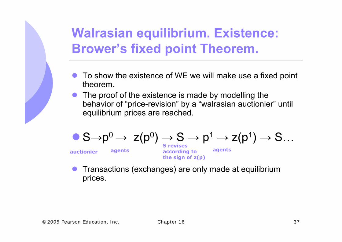
To show the existence of WE we will make use a fixed pointtheorem.The proof of the existence is made by modelling thebehavior of “price-revision” by a “walrasian auctionier” untilequilibrium prices are reached.
S→p0 → z(p0) → S → p1 → z(p1) → S…
Transactions (exchanges) are only made at equilibriumprices.
agentsS revises according tothe sign of z(p)
agentsauctionier
Chapter 16 38©2005 Pearson Education, Inc.
Walrasian equilibrium. Existence: Brower’s fixed point Theorem.
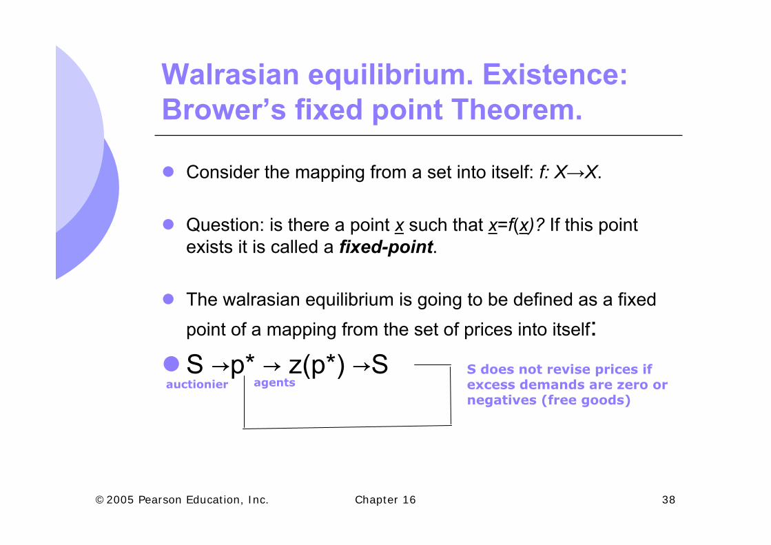
Consider the mapping from a set into itself: f: X→X.
Question: is there a point x such that x=f(x)? If this point exists it is called a fixed-point.
The walrasian equilibrium is going to be defined as a fixed point of a mapping from the set of prices into itself:S →p* → z(p*) →S
auctionier agentsS does not revise prices ifexcess demands are zero ornegatives (free goods)
Chapter 16 39©2005 Pearson Education, Inc.
Walrasian equilibrium.Brower’s fixed point Theorem.
Brower’s fixed point Theorem: Let S be a convexand compact (closed and bounded) subset ofsome euclídean space and let f be a continuousfunction, f: S→S, then there is at least an x in Ssuch that f(x)= x.
Notice:The Theorem is not about unicity. The Theorem gives sufficient conditions for theexistence of fixed points.
Chapter 16 40©2005 Pearson Education, Inc.
Walrasian equilibrium. Brower’sfixed point Theorem.
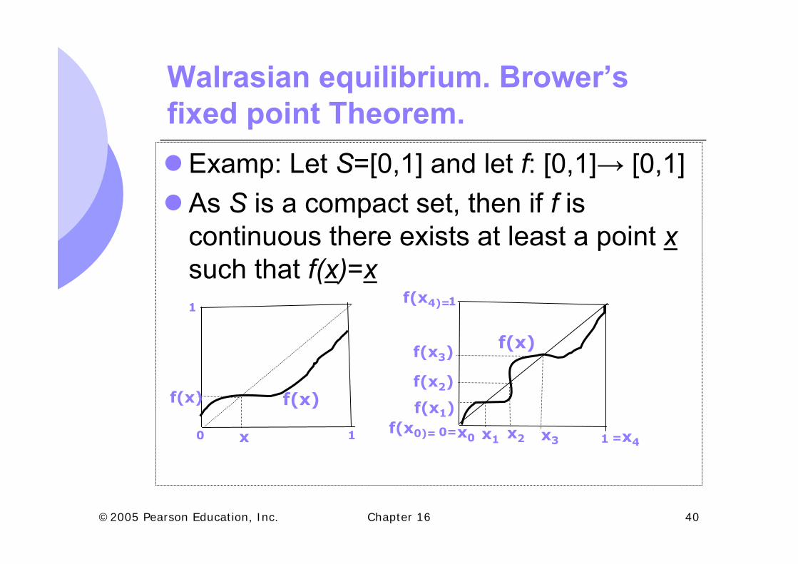
Examp: Let S=[0,1] and let f: [0,1]→ [0,1]As S is a compact set, then if f iscontinuous there exists at least a point xsuch that f(x)=x
f(x)
x0 1
1
0=
1
1 =x4
f(x)
f(x)
x0 x1 x2 x3
f(x4)=
f(x0)=
f(x3)
f(x2)
f(x1)
Chapter 16 41©2005 Pearson Education, Inc.
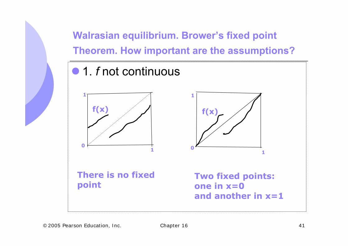
Walrasian equilibrium. Brower’s fixed pointTheorem. How important are the assumptions?
1. f not continuous
01
1
0
1
1
There is no fixedpoint
Two fixed points: one in x=0 and another in x=1
f(x) f(x)
Chapter 16 42©2005 Pearson Education, Inc.
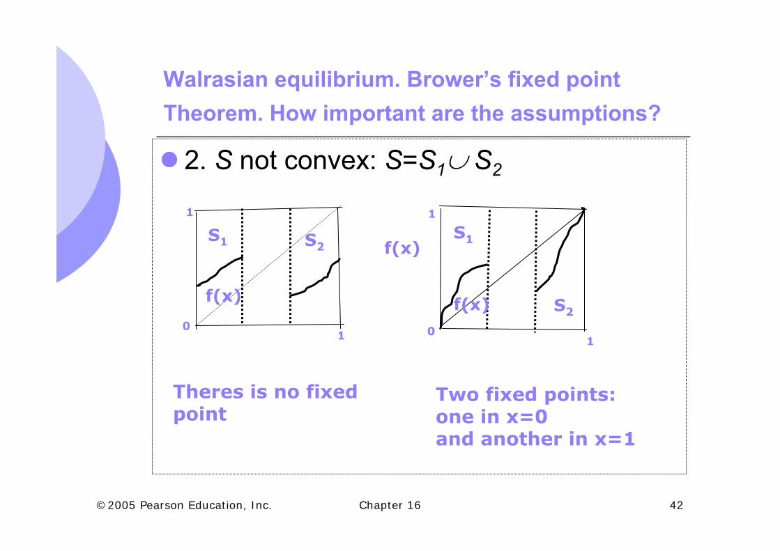
Walrasian equilibrium. Brower’s fixed pointTheorem. How important are the assumptions?
2. S not convex: S=S1∪ S2
01
1
0
1
1
Theres is no fixedpoint
Two fixed points: one in x=0 and another in x=1
f(x)
f(x)S1 S2
S1
S2f(x)
Chapter 16 43©2005 Pearson Education, Inc.
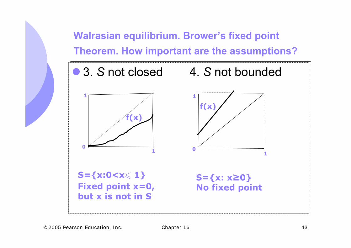
Walrasian equilibrium. Brower’s fixed pointTheorem. How important are the assumptions?
3. S not closed 4. S not bounded
01
1
0
1
1
S={x:0<x6 1}Fixed point x=0, but x is not in S
S={x: x≥0} No fixed point
f(x)f(x)
Chapter 16 44©2005 Pearson Education, Inc.
Walrasian equilibrium. ExistenceThe WE existence proof is based on the application of Brower fixed pointTheorem to our problem→To look for set S (convex and compact).1. The price set P (the set of vectors (p1, …,pk) with non-negativeelements) is not compact:
Is bounded from below: pl≥0, for all l=1,…,k, but not from above. It is a closed set. Then P is not compact.
2. “Normalize” the set of prices P to make it a compact set: eachabsolute price pl’ is substituted by a normalized pl:
with ∑lpl=1. For instance: p1’=4 and p2’=6 →p1=4/10=0.4 and p2=6/10=0.6 and p1+p2=1. (relative prices)
1
'
'
ll k
jj
ppp
=
=
∑
Chapter 16 45©2005 Pearson Education, Inc.
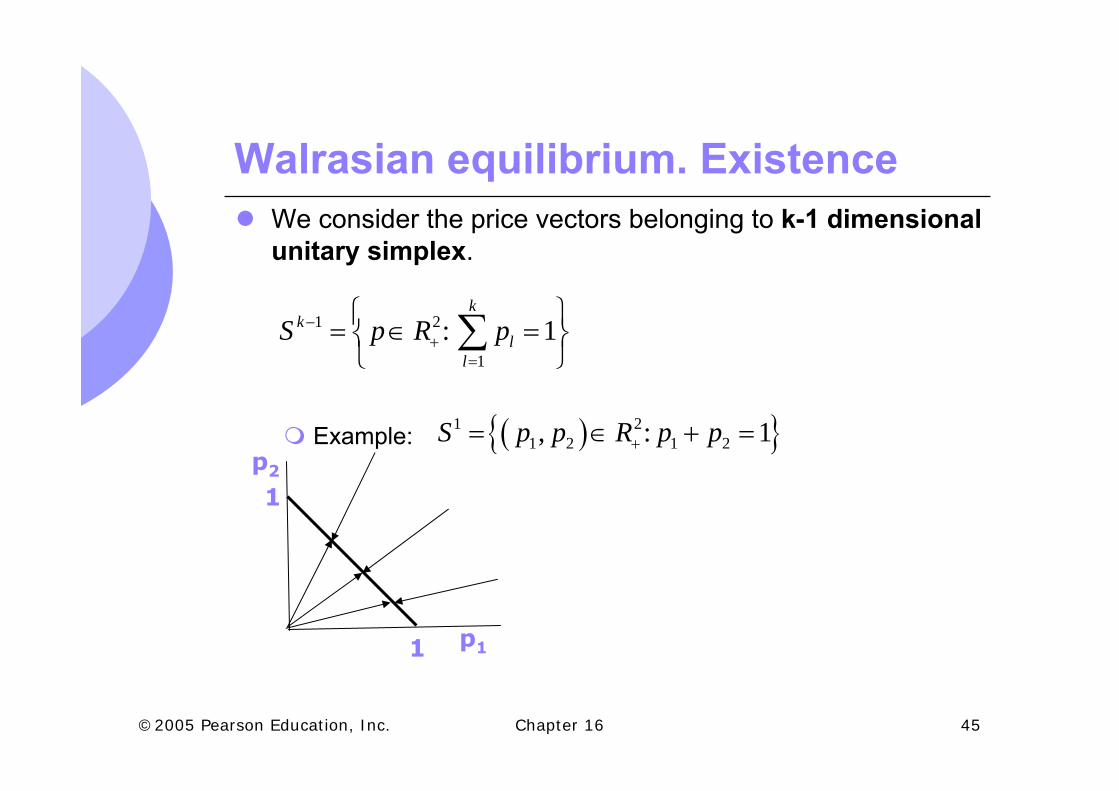
Walrasian equilibrium. ExistenceWe consider the price vectors belonging to k-1 dimensional unitary simplex.
Example:
1 2
1: 1
kk
ll
S p R p−+
=
⎧ ⎫= ∈ =⎨ ⎬
⎩ ⎭∑
( ){ }1 21 2 1 2, : 1S p p R p p+= ∈ + =
p2
p1
1
1
Chapter 16 46©2005 Pearson Education, Inc.
Walrasian equilibrium. Existence
Set Sk-1 (the normalized set of prices) is:bounded: pl≥0 y pl61, for all l=1,…,kclosed: {0,1} belong to Sk-1
convex: if p’ and p’’ are in Sk-1 (implying that∑lpl’=1 and ∑lpl’’=1), then:p=λp’+(1-λ)p’’ is in Sk-1, since∑lpl=∑lλpl’+∑l(1-λ)pl’’=λ ∑lpl’+ (1-λ) ∑lpl’’=1
Chapter 16 47©2005 Pearson Education, Inc.
Walrasian equilibrium. Existence3. As z(p) (and the demand functions) is homogeneous ofdegree zero in prices, prices can be normalized anddemands can be expressed as functions of relative prices. z(p1,p2,…,pk)= z(tp’1,tp’2,…,tp’k)= z(p’1,p’2,…,p’k), witht=1/∑jpj’. 4. A potential problem: z(p) is continuous whenever pricesare strictly positive.If some pj=0, by monotonicity of preferences, demands willbe infinite→”discontinuity”→z(p) could be not well-defined in the simplex boundaries.
Solution to the problem:Modify the non-satiation (monotonicity) assumption: “There exist satiation levels for all goods, butthere is always, at least, a good which is bought by theconsumer and such that the consumer is never satiated of it”.
Chapter 16 48©2005 Pearson Education, Inc.
Walrasian equilibrium. Existence. Walras’ Law
Walras’ Law (“identity”): For any p in Sk-1 , it is satisfied thatpz(p)=0, i.e., the value of the excess demand function is identicallyequal to zero.
Proof:pz(p)=p(∑ixi(p,pwi)-∑iwi)=∑i( pxi(p,pwi)-pwi)= ∑i0=0.
Consequences of Walras’ Law:a) If for all p»0, k-1 markets clear, then market k will also clear:p1z1+p2z2=0 by LW, p1>0 y p2>0, if z1=0, LW→z2=0
b) Free goods: if p* is a WE and zj(p)<0, then pj*=0,in words if in a WE a good has excess supply, then this good will be free:p1z1+p2z2=0 by LW, if z2<0, LW →p2=0.
Chapter 16 49©2005 Pearson Education, Inc.
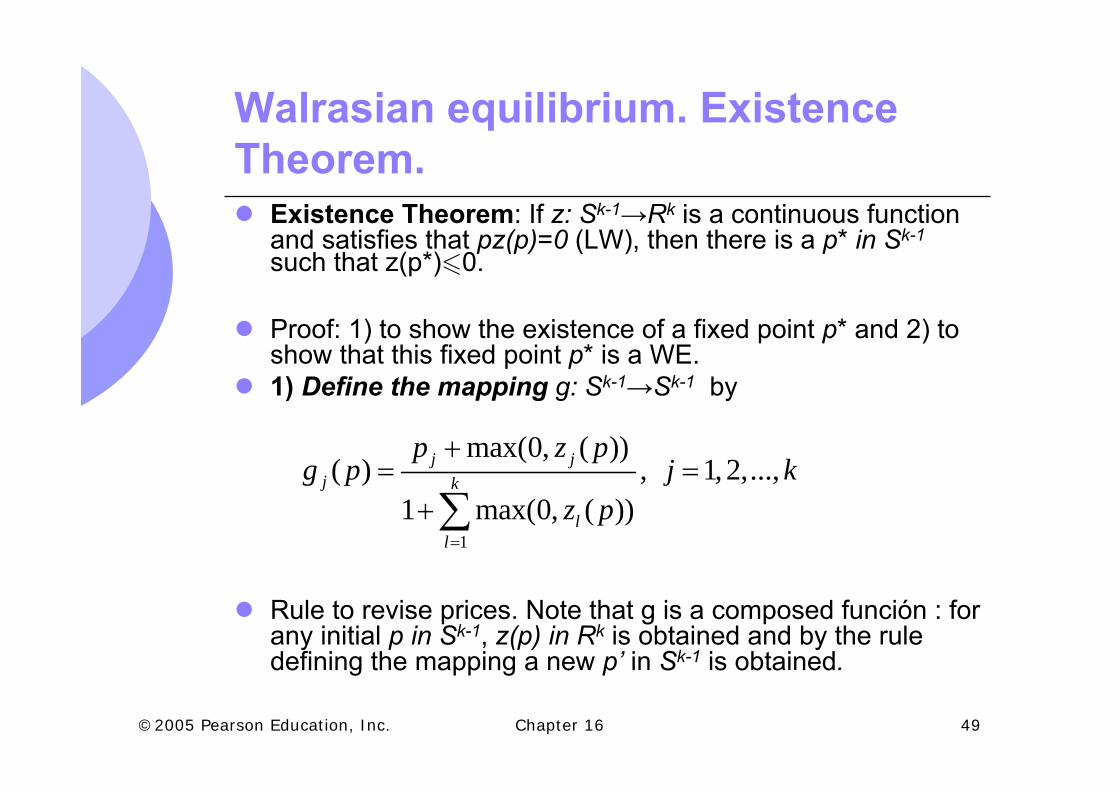
Walrasian equilibrium. ExistenceTheorem.
Existence Theorem: If z: Sk-1→Rk is a continuous functionand satisfies that pz(p)=0 (LW), then there is a p* in Sk-1
such that z(p*)60.
Proof: 1) to show the existence of a fixed point p* and 2) to show that this fixed point p* is a WE.1) Define the mapping g: Sk-1→Sk-1 by
Rule to revise prices. Note that g is a composed función : for any initial p in Sk-1, z(p) in Rk is obtained and by the rule defining the mapping a new p’ in Sk-1 is obtained.
1
max(0, ( ))( ) , 1, 2,...,
1 max(0, ( ))
j jj k
ll
p z pg p j k
z p=
+= =
+ ∑
Chapter 16 50©2005 Pearson Education, Inc.
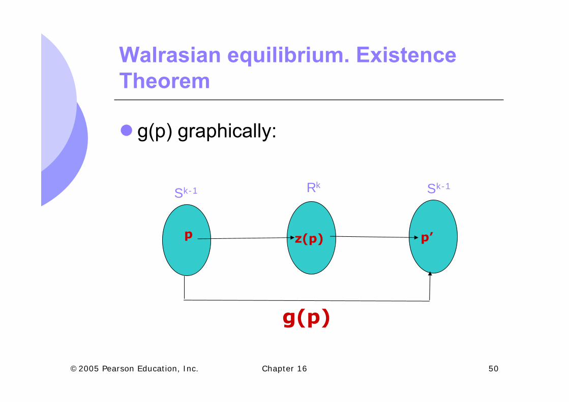
Walrasian equilibrium. ExistenceTheorem
g(p) graphically:
Sk-1 Sk-1Rk
p z(p) p’
g(p)
Chapter 16 51©2005 Pearson Education, Inc.
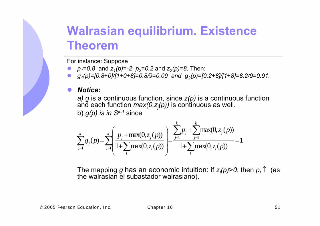
Walrasian equilibrium. ExistenceTheoremFor instance: Suppose
p1=0.8 and z1(p)=-2; p2=0.2 and z2(p)=8. Then:g1(p)=[0.8+0]/[1+0+8]=0.8/9=0.09 and g2(p)=[0.2+8]/[1+8]=8.2/9=0.91.
Notice:a) g is a continuous function, since z(p) is a continuous functionand each function max(0,zj(p)) is continuous as well. b) g(p) is in Sk-1 since
The mapping g has an economic intuition: if zl(p)>0, then pl ↑ (as the walrasian el subastador walrasiano).
1 1
1 1
max(0, ( ))max(0, ( ))
( ) 11 max(0, ( )) 1 max(0, ( ))
k k
j jk kj j j j
jj j l l
l l
p z pp z p
g pz p z p
= =
= =
+⎛ ⎞+⎜ ⎟= = =⎜ ⎟+ +⎜ ⎟
⎝ ⎠
∑ ∑∑ ∑ ∑ ∑
Chapter 16 52©2005 Pearson Education, Inc.
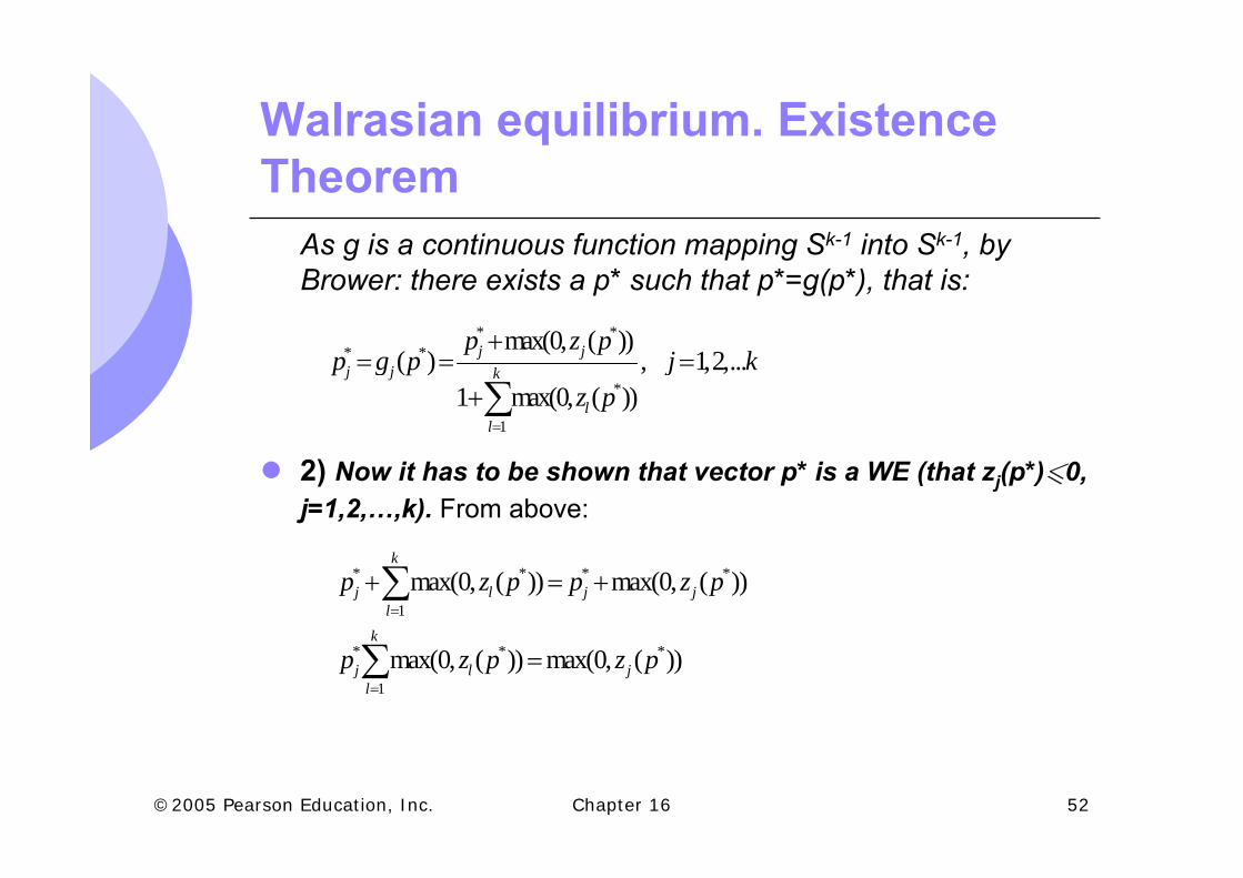
Walrasian equilibrium. ExistenceTheorem
As g is a continuous function mapping Sk-1 into Sk-1, by Brower: there exists a p* such that p*=g(p*), that is:
2) Now it has to be shown that vector p* is a WE (that zj(p*)60, j=1,2,…,k). From above:
* ** *
*
1
max(0, ( ))( ) , 1,2,...
1 max(0, ( ))
j jj j k
ll
p z pp g p j k
z p=
+= = =
+∑
* * * *
1
* * *
1
max(0, ( )) max(0, ( ))
max(0, ( )) max(0, ( ))
k
j l j jl
k
j l jl
p z p p z p
p z p z p
=
=
+ = +
=
∑
∑
Chapter 16 53©2005 Pearson Education, Inc.
Walrasian equilibrium. ExistenceTheorem
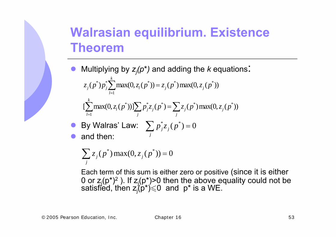
Multiplying by zj(p*) and adding the k equations:
By Walras’ Law:and then:
Each term of this sum is either zero or positive (since it is either0 or zj(p*)2 ). If zj(p*)>0 then the above equality could not be satisfied, then zj(p*)60 and p* is a WE.
* * * * *
1
* * * * *
1
( ) max(0, ( )) ( )max(0, ( ))
[ max(0, ( ))] ( ) ( )max(0, ( ))
k
j j l j jl
k
l j j j jl j j
z p p z p z p z p
z p p z p z p z p
=
=
=
=
∑
∑ ∑ ∑* *( ) 0j j
jp z p =∑
* *( ) max(0, ( )) 0j jj
z p z p =∑