Waiwhetu Outfall Dilution Assessment

Report

October 2017

Waiwhetu Outfall Options - Dilution

Assessment

Numerical Modelling

waiwhetu outfall dilution assessment / bjt / 2017-10-30

This report has been prepared under the DHI Business Management System

certified by Bureau Veritas to comply with ISO 9001 (Quality Management)

DHI Water and Environment Ltd• ecentre, Gate 5, Oaklands Road• Albany 0752 Auckland• New Zealand• Telephone: +64 9 912 9638 • Telefax: • [email protected]• www.dhigroup.com

Waiwhetu Outfall Options - Dilution

Assessment

Numerical Modelling

Prepared for Wellington Water

Represented by Anna Bridgman (Stantec) Hutt River Mouth

Project manager Benjamin Tuckey

Project number 44801116

Approval date 30/10/2017

Revision Final 1.1

Classification Open

waiwhetu outfall dilution assessment / bjt / 2017-10-30

i

CONTENTS

1 Executive Summary .................................................................................................... 1

2 Introduction ................................................................................................................. 2 2.1 Project Appreciation ....................................................................................................................... 2 2.2 Objectives of Proposed Study ........................................................................................................ 4 2.3 Co-ordinate System and Vertical Datum ....................................................................................... 4

3 Overview of Data ......................................................................................................... 5 3.1 Current, Water Level and CTD Data from NIWA Data Collection Campaign ................................ 5 3.1.1 Measurement schedule .................................................................................................................. 5 3.1.2 Mooring Deployments .................................................................................................................... 7 3.1.3 CTD Casts ...................................................................................................................................... 9 3.2 Flow and Water Level Data .......................................................................................................... 12 3.3 Bathymetric Data.......................................................................................................................... 13 3.4 Wind Data .................................................................................................................................... 15

4 Study Approach and Scenario Selection ................................................................. 17 4.1 Overview of Mixing Behaviour ..................................................................................................... 17 4.2 Near-Field and Far-Field Models ................................................................................................. 17 4.3 Scenario Selection ....................................................................................................................... 18

5 Far-Field Model Set Up and Calibration ................................................................... 20 5.1 Set Up .......................................................................................................................................... 20 5.1.1 Bathymetry and Mesh .................................................................................................................. 20 5.1.2 Open Ocean Boundaries ............................................................................................................. 21 5.1.3 Freshwater Inflows ....................................................................................................................... 21 5.1.4 Wind ............................................................................................................................................. 21 5.1.5 Wastewater Representation ......................................................................................................... 22 5.2 Calibration .................................................................................................................................... 22 5.2.1 Water Levels and Currents .......................................................................................................... 22 5.2.2 Salt Wedge and River Plume ....................................................................................................... 28

6 Near-Field Assessment ............................................................................................. 31 6.1 Wastewater Properties and Outfall Arrangement ........................................................................ 31 6.2 Receiving Water Conditions ......................................................................................................... 31 6.2.1 Receiving Water Level, Flow and Salinity .................................................................................... 31 6.2.2 Receiving Water Bathymetry ....................................................................................................... 32 6.2.3 Situations where Modifications of Assumptions were Required to Obtain Dilution

Predictions ................................................................................................................................... 34 6.3 Model Results .............................................................................................................................. 34

7 Far-Field Assessment ............................................................................................... 39 7.1 Model Results .............................................................................................................................. 39

ii waiwhetu outfall dilution assessment / bjt / 2017-10-30

8 Summary ................................................................................................................... 62

9 References ................................................................................................................ 64

Executive Summary

1

1 Executive Summary

A wastewater plume dispersion study was undertaken for the existing wastewater overflow from

the Seawater Wastewater Treatment Plant into Waiwhetu Stream and for two potential

alternative wastewater overflows. The three locations for which the assessment was undertaken

were:

Option A - existing location in Waiwhetu Stream;

Option B - Hutt River (near Waiwhetu Stream mouth) close to the water surface; and

Option C - Hutt River (100 m off Barnes Street) on the sea bed.

The performance of each outfall location was assessed by determining the plume dilution that

will occur for a range of selected discharge, hydrodynamic and climate scenarios (a total of 25

scenarios) at sensitive sites within the river mouth and Wellington harbour. Both neap and

spring tidal conditions were considered, along with calm, southerly and northerly wind

conditions.

Predicted 1st, 5th, 25th and 50th percentile dilutions at the sensitive sites were calculated for each

scenario and outfall option. Percentile plots at the sensitive sites were also generated for a 30

day simulation including range of representative wind conditions within the harbour, to provide

an indication of the visitation frequency of the plume from each outfall at the sites.

Generally Outfall C produced the most dilution of the wastewater plume compared with other

potential outfall locations, before visitation of the plume occurred at the sensitive sites, while

Outfall B generally performed slightly better than Outfall A, however not for all conditions or

sites.

2 waiwhetu outfall dilution assessment / bjt / 2017-10-30

2 Introduction

Stantec New Zealand (Stantec) on behalf of Wellington Water (WW) have commissioned DHI

Water and Environment Ltd (DHI) to undertake a plume dispersion study for the existing

wastewater overflow from the Seawater Wastewater Treatment Plant into Waiwhetu Stream and

for two alternative wastewater overflow, to form part of an Assessment of Environmental Effects

(AEE).

NIWA originally undertook a plume dispersion study for Hutt City Council for the existing

wastewater overflow and potential alternative discharge sites (NIWA, 2015). However, the

selected modelling approach resulted in a model of Wellington Harbour which did not cover the

Hutt River mouth in sufficient detail to provide a comparative assessment of the dilutions for

each option considered.

DHI have previously undertaken a preliminary dilution assessment for a number of outfall

options (DHI, 2011) and a near-field dilution assessment based on receiving environment

information provided by NIWA (DHI, 2016).

2.1 Project Appreciation

For the majority of the time, treated wastewater effluent from the Seaview Wastewater

Treatment Plant discharges through a short outfall south of Pencarrow Head into the open

ocean outside Wellington Harbour. On occasions, when maintenance is carried out on the

outfall or when the capacity of the outfall is exceeded, treated wastewater effluent is discharged

into the Waiwhetu Stream, which flows into the Hutt River.

A plume dispersion study was required to investigate the potential for discharging from the

existing overflow location and two other possible future alternatives in the Hutt River, as shown

in Figure 2-1 and outlined below:


Option B - Hutt River (near Waiwhetu Stream mouth) close to the water surface; and


The salt wedge which propagates up the lower Hutt River on the incoming tide will have an

influence on the mixing of the discharged wastewater and must be considered for a wastewater

dilution assessment.

The potential discharge considered were as follows:

unplanned pipe repair that would result in a typical dry weather discharge rate of

0.55 m3/s (1.10 m3/s for Option B on outgoing tide) for a duration of 5 days;

planned maintenance works that would result in a typical dry weather discharge rate of

0.55 m3/s (1.10 m3/s for Option B on outgoing tide) for a duration of 30 days;

wet weather overflows typically discharging at a rate of 0.8 m3/s for a duration of 1 day;

wet weather occurring while the main outfall pipeline is out of operation that would result

in a peak flow up to 3 m3/s for duration of 1 day.

3

Figure 2-1 Existing wastewater outfall (Option A) and potential wastewater outfalls Options B and C near the mouth of the Hutt River.

The performance of each outfall location was assessed by determining the plume dilution that

will occur for selected discharge, hydrodynamic and climate scenarios at the following sensitive

sites (presented in Figure 2-2):

Petone Beach west;

Petone Beach east;

Waione Street Bridge;

100m downstream of Hutt/Waiwhetu confluence;

Lowry Bay;

Days Bay;

Port Road corner beach; and

Seaview Marina.


Figure 2-2 Location of sensitive sites for plume dilution assessment.

2.2 Objectives of Proposed Study

The specific objectives of the study were:

1. Calibrate and validate a three dimensional hydrodynamic model capable of replicating

saline intrusion behaviour within the Waiwhetu Stream and Hutt River and predict

currents and water levels within vicinity of the potential outfalls;

2. Identify appropriate hydrodynamic scenarios for assessing wastewater plume dilutions

from the potential outfalls;

3. For selected discharge and hydrodynamic scenarios, undertake a near-field assessment

to determine wastewater plume dilutions from the potential outfalls within the zone of

near-field mixing; and

4. For selected discharge, hydrodynamic and climate scenarios, undertake a far-field

assessment to determine wastewater plume dilutions at sensitive sites for each of the

outfalls.

2.3 Co-ordinate System and Vertical Datum

For this study, all data is presented using the New Zealand Transverse Mercator projection and

the vertical datum is referenced to Wellington Mean Sea Level datum.

5

3 Overview of Data

This section provides an overview of the data that was collected by NIWA specifically for this

study (NIWA, 2013) and describes additional data DHI have utilised for this study.

3.1 Current, Water Level and CTD Data from NIWA Data Collection Campaign

3.1.1 Measurement schedule

During May to July 2013, NIWA deployed an Acoustic Doppler Current Profilers (ADCP) and

bed-level sensors at three mooring locations and undertook Conductivity, Temperature and

Depth (CTD) casts at 12 station location on five days. An overview of the data collection

locations is presented in Figure 3-1, while Table 3-1 presents an overview of the schedule of the

data collection.

Figure 3-1 NIWA moorings and CTD cast station locations (1-12), in the vicinity of the Hutt River mouth and Somes Island, where data was collected between May-July 2013.


Table 3-1 Schedule of the NIWA data collection campaign (only data used in this study).

7

3.1.2 Mooring Deployments

During May, June and July 2013, NIWA deployed ADCP and bed-level temperature, salinity and

pressure (MicroCat) sensors at three locations (see Figure 3-1):

2 km south of Somes Island (referred to as the Harbour mooring);

one 150 m offshore from 77 Port Road (referred to as the River mouth mooring); and

one 130 m downstream of the Waione Street bridge across the Hutt River (referred to

as the River mooring).

The ADCP at the River mouth mooring was lost and so provided no data, however the bed-level

measurements were recovered. Bed-level salinity measurements at the three NIWA mooring

locations are presented in Figure 3-2. Measurements indicate that the salinity in the harbour

remains approximately constant over time and that Hutt River flows, with a salinity of

approximately 0.0 PSU, are capable of flushing saltwater from the lower river right to the bed for

extended periods of time. NIWA note that River mouth mooring measurements (the green line in

Figure 3-2) from 21st June onwards are dubious because of possible clogging of the

measurement device. Further details concerning the data collection can be found in NIWA

(2013).

Figure 3-3 presents a comparison of the instantaneous salinity at the sea bed in the river and

the river mouth compared with the CTD cast data at the sea bed (see Section 3.1.3). CTD cast 5

was located close to the River salinity mooring, while CTD cast 8 was located close to the River

mouth mooring. It has to be assumed that CTD casts data is more accurate. There is a large

discrepancy for both sets of data. On 7th June and 9th July, with CTD cast 5 recording a salinity

of 34 PSU at seabed, while the river mooring recorded a salinity of 0 PSU. On 9th July the CTD

cast 8 recorded a salinity of 34 PSU at seabed, while the river mouth mooring recorded a salinity

of 0 PSU. It would appear that measurements from both deployed instruments in the river are

dubious and therefore it wasn’t possible to use data for this study.


Figure 3-2 Bed-level salinity measurements at the three NIWA mooring locations.

Figure 3-3 Bed-level salinity measurements at the NIWA river mooring locations compared with CTD cast data.

9

3.1.3 CTD Casts

NIWA undertook nine sets of CTD casts at 12 station locations (see Figure 3-1), on the following

five days:

9th May;

7th June;

12th June;

14th June; and

9th July 2013.

The data for all but the first set of casts has been provided to DHI. The timings of the casts

compared with water levels at Hutt River Estuary Bridge are presented in Figure 3-4. The casts

covered most parts of the tide apart from mid to low tide for the outgoing tide. The approximate

wind condition (see Section 3.4) and Hutt River flow (see Section 3.2) at the time of the CTD

casts is presented in Table 3-2.

In addition, NIWA undertook a longitudinal “spatial” survey, at a depth of 0.5 m, from the rail

bridge to 300 m downstream of the River mouth mooring and back again over a period of 1.75

hours. DHI has not made use of this data.

Figure 3-4 Water levels at Hutt River at Estuary Bridge with times of CTD casts.


Table 3-2 Approximate wind condition and Hutt River flow at the time of the CTD casts.

Date of CTD Casts Approximate Wind Approximate Hutt River Flow

7th June Gentle northerly breeze 15 m3/s

12th June Moderate to fresh southerly breeze 11 m3/s

14th June Moderate to fresh southerly breeze 13 m3/s

9th July Moderate to fresh northerly breeze 23 m3/s

Transects plots are presented in Figure 3-5, produced by interpolating between the CTD casts

at stations 1, 3, 4, 5, 6, 8, 9, 10, 11 and 12. These provide an instantaneous overview of the salt

wedge behaviour when the set of CTD casts were carried out. There are anomalies in the

collected data at Station 2. Station 7 is located only 66 m from Station 6, close to the Waiwhetu

confluence. These CTD casts were not used.

Outfall B is located at approximately 1,700 m while Outfall C is located at approximately

2,150 m. The salt wedge is always present at both potential outfall locations, for periods when

CTD casts were undertaken.

It is also interesting to note that even during a moderate to fresh southerly breeze, where it is

observed that the river plume is ultimately transported anti clockwise around the harbour1, the

CTD casts on 12th and 14th June indicate that the river plume initially travels southwards along

the direction of the CTD transects. This observation maybe due to a combination of the

momentum of the river plume as it exits the river and the river mouth being sheltered from

southerly wind events and beyond the CTD casts, wind forcing would start to drive the behaviour

of the river plume. The field notes from NIWA provided with the CTD casts (NIWA, 2013),

support this assumption. NIWA noted that CTD cast station 11 was much more exposed to wind

than upstream casts.

Further details concerning the data collection can be found in NIWA (2013).

1 Plume is transported south down eastern side of harbour during northerly wind (Heath, 1977).

11

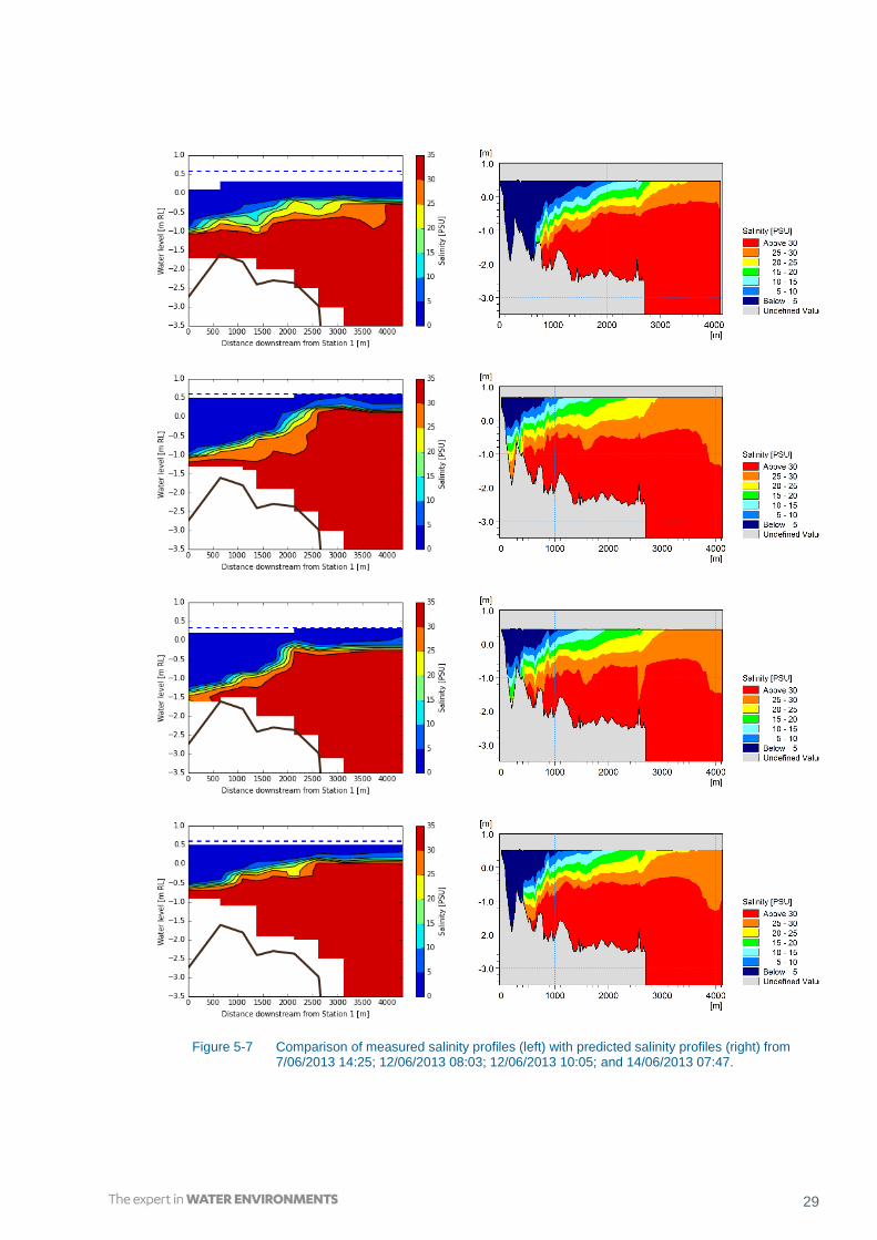
Figure 3-5 Measured salinity profiles between Station 1 and Station 12. Collection period (from left to right and top to bottom): from 7/06/2013 14:25 over 76 min; from 12/06/2013 08:03 over 72 min; from 12/06/2013 10:05 over 52 min; from 14/06/2013 07:47 over 54 min; from 14/06/2013 09:29 over 45 min; from 14/06/2013 10:55 over 53 min; from 9/07/2013 14:08 over 67 min; and from 9/07/2013 16:06 over 59 min.


3.2 Flow and Water Level Data

The following flow and water level data was obtained from the Greater Wellington Regional

Council live monitoring site for the period 1st May to 2nd August 2013 to cover the period of

NIWA data collection:

1. Hutt River at Taita Gorge flow;

2. Hutt River at Estuary Bridge water level;

3. Waiwhetu Stream at White Line East flow; and

4. Wellington Harbour at Queens Wharf water level.

Time series for data in the vicinity of Hutt River are presented in Figure 3-6.

Figure 3-6 GWRC discharge and water level gauging data for the lower Hutt River and Waiwhetu Stream.

13

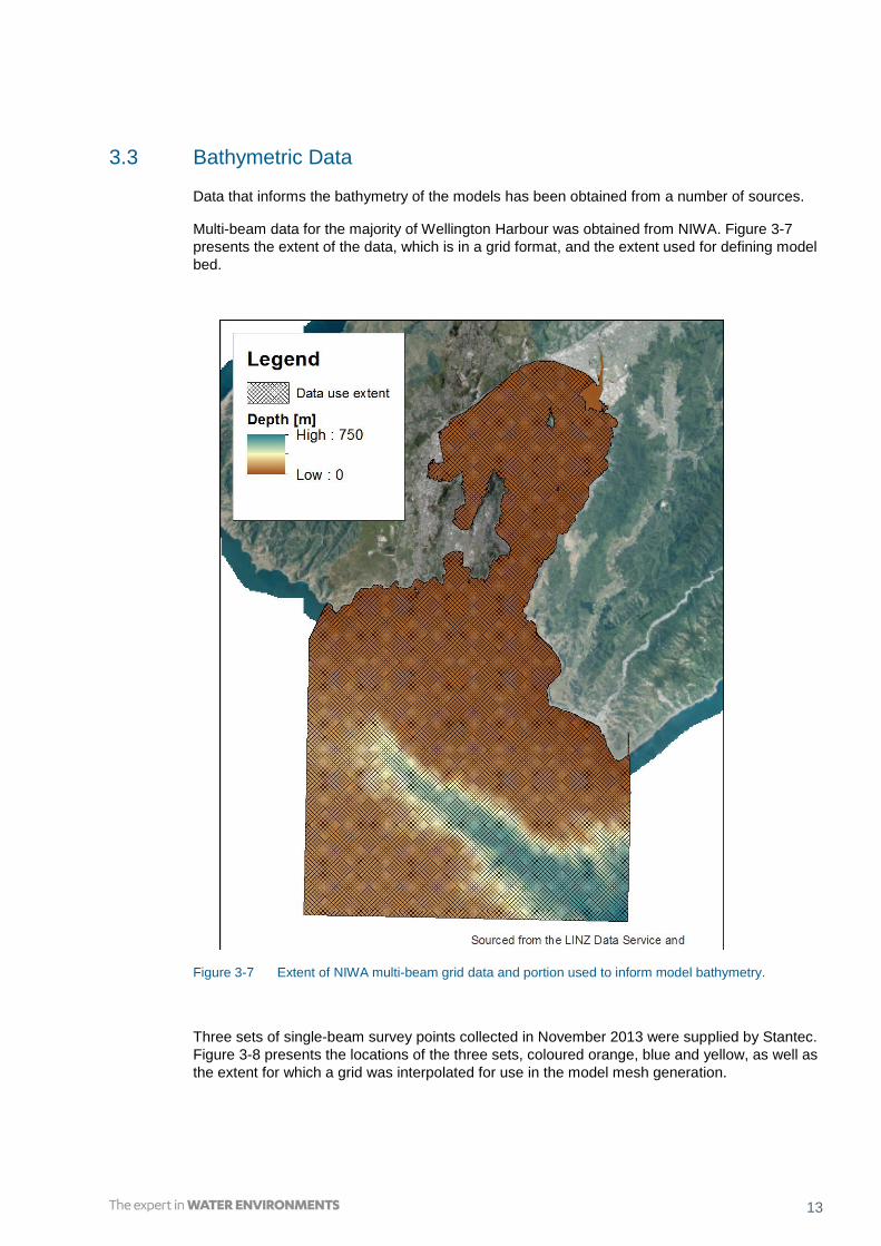
3.3 Bathymetric Data

Data that informs the bathymetry of the models has been obtained from a number of sources.

Multi-beam data for the majority of Wellington Harbour was obtained from NIWA. Figure 3-7

presents the extent of the data, which is in a grid format, and the extent used for defining model

bed.

Figure 3-7 Extent of NIWA multi-beam grid data and portion used to inform model bathymetry.

Three sets of single-beam survey points collected in November 2013 were supplied by Stantec.

Figure 3-8 presents the locations of the three sets, coloured orange, blue and yellow, as well as

the extent for which a grid was interpolated for use in the model mesh generation.


Figure 3-8 Single-beam bed survey points collected in November 2013 in the vicinity of the Hutt River mouth.

Cross section survey points for the Hutt River and Waiwhetu Stream were provided by Stantec.

Figure 3-9 presents the locations of the Hutt River survey points, coloured red, and Waiwhetu

Stream survey points, coloured yellow, as well as the extent for which a grid was interpolated for

use in the model mesh generation.

Figure 3-9 Hutt River and Waiwhetu Stream cross section survey points.

15

In the vicinity of the Hutt River and Waiwhetu Stream confluence the bathymetry has been

modified manually in order to connect the bed levels of the stream and river in a realistic way.

The survey of spot heights undertaken on 17th February 2015, provided by Stantec, did not

agree sufficiently with the river and stream surveys and so has not been used for this study.

3.4 Wind Data

The following sets of wind data were obtained from NIWA’s climate database (cliflo.niwa.co.nz):

Hourly wind observations from Kaukau weather station (north of Wellington Harbour) for

the period January 2000 to January 2012. There was no data freely available after this

date.

Hourly wind observations from Baring Head weather station (south of Wellington

Harbour) for the period April 2007 to April 2017.

The wind station at the Kaukau is located 425 m above Mean Sea Level (MSL) and the wind

station at Baring Head is 79 m above MSL. The wind data was scaled to 10 m above MSL using

the following formula (Ahrens, 2003):

𝑊𝑆2 = 𝑊𝑆1 × 𝑙𝑛(

𝑍2𝑍𝑜

⁄ )

𝑙𝑛(𝑍1

𝑍𝑜⁄ )

Where WS2 = wind speed at height Z2 (m/s);

WS1 = wind speed at height Z1 (m/s); and

Zo = aerodynamic roughness length (m).

For the ocean Zo = 0.0002 m, therefore to scale wind speeds from 425 m to 10 m the scaling

factor is 0.83 and from 79 m to 10 m, the scaling factor is 0.88.

To provide a direct comparison of the wind data, wind roses for the period January 2008 to

January 2013 for both sets of wind observations are presented in Figure 3-10.

The wind pattern behaviour at both locations is very similar, with both locations experiencing

predominant northerly and southerly winds (although with a slight difference in alignment of

approximately 10°). The Kaukau wind data was selected as most representative of northern

Wellington Harbour.

To assist in defining scenarios for simulations, the wind data was analysed (see Table 3-3) to

assess the 25th, 50th and 90th percentiles for southerly (180 ± 30°) and northerly winds (360 ±

30°). Wind speeds less than 2.5 m/s were considered calm (although strictly a light breeze) and

discounted. An analysis of the frequency of the wind from these directions from the Kaukau data

was performed and is shown in Table 3-4.


Figure 3-10 Wind data from Kaukau (left) and Baring Head (right) for period January 2008 to January 2013.

Table 3-3 25th, 50th and 90th percentiles for dominant wind directions of Kaukau wind data.

Wind Speed (m/s)

Southerly Wind (180 ± 30°) Northerly Wind (360 ± 30°)

25th Percentile 6.1 6.9



Table 3-4 Occurrence of dominant wind directions.

Direction Occurrence

Calm (< 2.5 m/s) 7%

Southerly (180 ± 30°) 27%

Northerly (360 ± 30°) 50%

Other 15%

17

4 Study Approach and Scenario Selection

This section outlines the overall approach that was taken for this study and provides information

on the scenarios that have been investigated.

4.1 Overview of Mixing Behaviour

The discharged wastewater plumes will mix and dilute due to two types of mixing processes:

Near-field mixing. This refers to dilution of the wastewater discharge as it enters the

marine environment in a jet or plume like flow. In this area the flow and mixing is

determined by the discharge itself, i.e. the excess momentum and buoyancy in the jet-

like flow. Near-field mixing occurs due the entrainment of the surrounding ambient

water into the jet-like flow.

Far-field mixing. This refers to where the plume dynamics are governed by the

conditions in the surrounding water, here predominantly currents and turbulence

induced by density gradients.

Different types of models are required for assessing each phase of mixing.

4.2 Near-Field and Far-Field Models

The first modelling stage (near-field) involved the use of a dedicated near-field model, here the

empirically based Cornell Mixing Zone Expert System (CORMIX), to predict the dilution

characteristics of the near-field mixing zone. CORMIX is an industry standard tool which is well

suited for the prediction of plume geometry and entrainment based on positively/negatively

buoyant discharges, for single port or diffuser outfalls. Its main limitations relate to simplistic

assumptions regarding the spatial uniformity of the receiving water, and to the fact that both

discharge and ambient conditions are assumed to be stationary in time. The model is thus well

suited to describing plume behaviour immediately after release, but not its behaviour in a

dynamic environment.

The second modelling stage (far-field) involved the use of DHI’s fully dynamic 3-dimensional

flow and transport modelling system MIKE 3 FM, which is suitable for use where three

dimensional density stratified flows are important as is the case for this study where the mixing

behaviour of a buoyant plume and saline intrusion within the lower Hutt River must be generally

reproduced. Further details of MIKE 3 FM model, can be found in the MIKE 3 FM User Manual

(DHI, 2017).

The flexible mesh allows for a varying resolution computational grid so that a finer resolution can

be used for areas of interest (i.e. Hutt River and outfall locations) and a lower resolution can be

used for other areas. This allows large savings in simulation times without compromising model

resolution in areas of interest. The vertical model resolution is based on discretisation in layers

of varying thickness, so called sigma layers. The main limitation for the MIKE 3 FM model is its

inability to efficiently describe initial small-scale mixing process in the immediate proximity of the

outfall, hence why a separate near-field model required.

To simulate the behaviour of the wastewater plume the advection-dispersion (AD) module was

used. The AD module simulates the spread of dissolved and suspended substances subject to

the transport process described by the HD module. The wastewater plume was defined as a

conservative tracer (i.e. no decay processes).


The hybrid application of the two models thus utilises the relative strengths of both systems,

while maintaining computational efficiency. The two models are indirectly coupled as the near-

field model will provide the initial conditions for the 3D model.

The CORMIX predictions were utilised to determine:

an appropriate resolution to use for the far-field model domain to obtain initial mixing

comparable with predictions from near-field model; and

the behaviour and characteristics of the plume at end of near-field mixing phase. As an

example, if near-field model predicted that wastewater plume did not fully vertically mix

throughout the water column and instead was trapped below the surface freshwater layer of

the salt wedge at end of near-field mixing phase, then this would need to be taken into

account when inputting the wastewater into the MIKE 3 FM model.

4.3 Scenario Selection

An overview of the scenarios selected for the dilution assessment for each outfall location is

presented in Table 4-1. These provide an envelope of the different, tidal, wind and outfall

discharge scenarios that may occur. For dry weather discharges, the Hutt River and Waiwhetu

Stream inflows were set to 25 m3/s and 0.3 m3/s respectively. For wet weather discharges,

constant flows of 100 m3/s and 2 m3/s for the Hutt River and Waiwhetu Stream respectively were

assumed. These river flows were selected with agreement from Stantec.

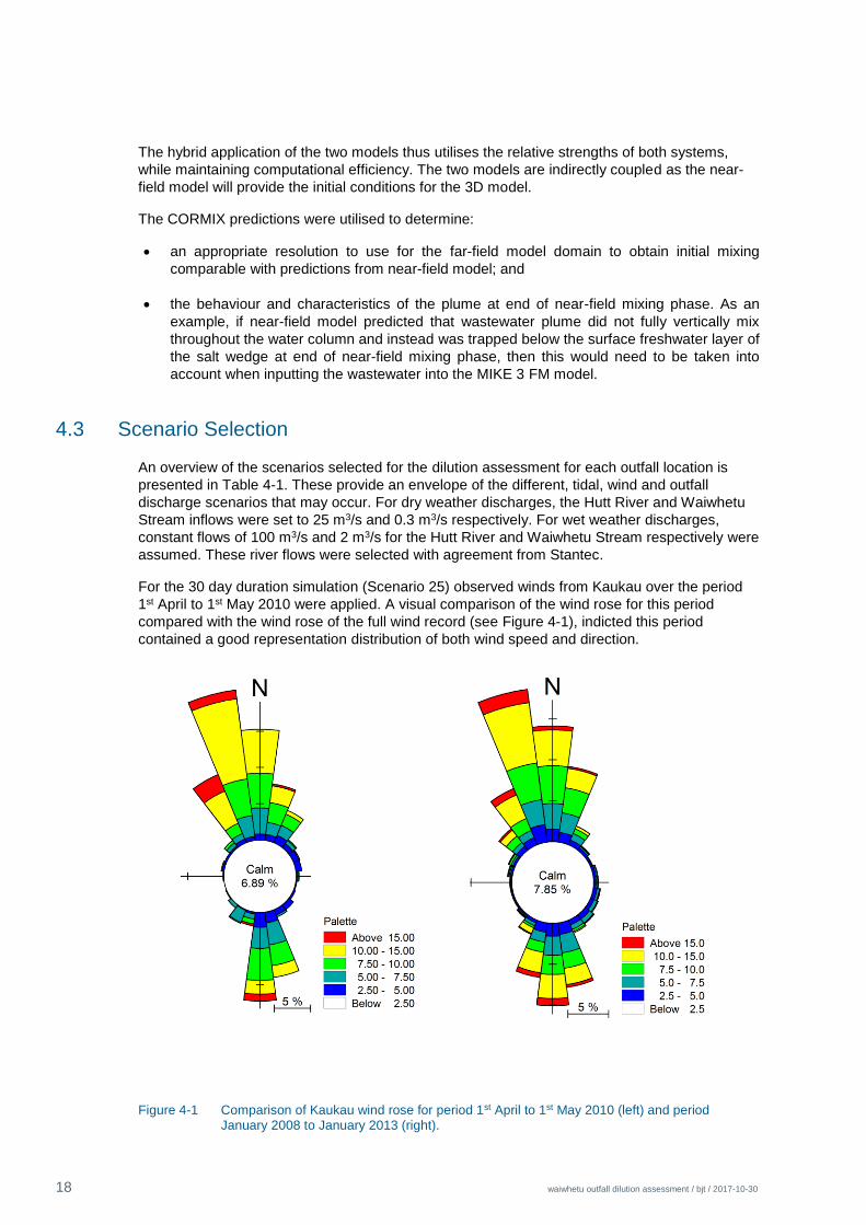
For the 30 day duration simulation (Scenario 25) observed winds from Kaukau over the period

1st April to 1st May 2010 were applied. A visual comparison of the wind rose for this period

compared with the wind rose of the full wind record (see Figure 4-1), indicted this period

contained a good representation distribution of both wind speed and direction.

Figure 4-1 Comparison of Kaukau wind rose for period 1st April to 1st May 2010 (left) and period January 2008 to January 2013 (right).

19

Table 4-1 Overview of selected scenarios.

Scenario Overflow

Discharge Rate

Duration of

Discharge

Wind Condition Tidal

Condition

1 0.55 m3/s

(1.10 m3/s for

Option B on

outgoing tide)

5 days Calm Neap

2 Spring

3 90th Percentile Southerly Neap

4 Spring

5 50th Percentile Northerly Neap

6 Spring


8 Spring

9 0.8 m3/s 1 day Calm Neap

10 Spring


12 Spring


14 Spring


16 Spring

17 3 m3/s 1 day Calm Neap

18 Spring


20 Spring


22 Spring


24 Spring

25 0.55 m3/s

(1.10 m3/s for

Option B on

outgoing tide)

30 days Kaukau wind - 1st April to 1st May 2010 N/A


5 Far-Field Model Set Up and Calibration

A three dimensional far-field model was developed that could reproduce both saline intrusion

within the lower Hutt River and the river, tidal and wind driven currents for the lower Hutt River

and northern Wellington Harbour. These are the important processes which will determine the

dilution and transport of the discharged wastewater plume.

5.1 Set Up

5.1.1 Bathymetry and Mesh

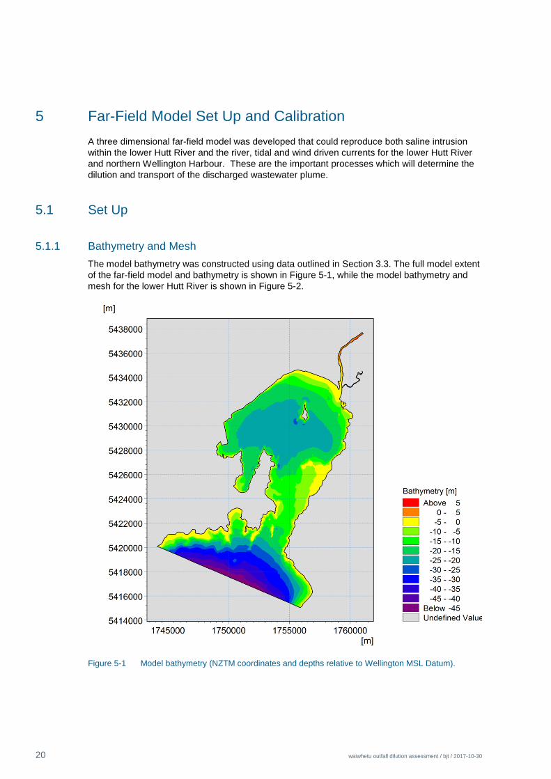
The model bathymetry was constructed using data outlined in Section 3.3. The full model extent

of the far-field model and bathymetry is shown in Figure 5-1, while the model bathymetry and

mesh for the lower Hutt River is shown in Figure 5-2.

Figure 5-1 Model bathymetry (NZTM coordinates and depths relative to Wellington MSL Datum).

21

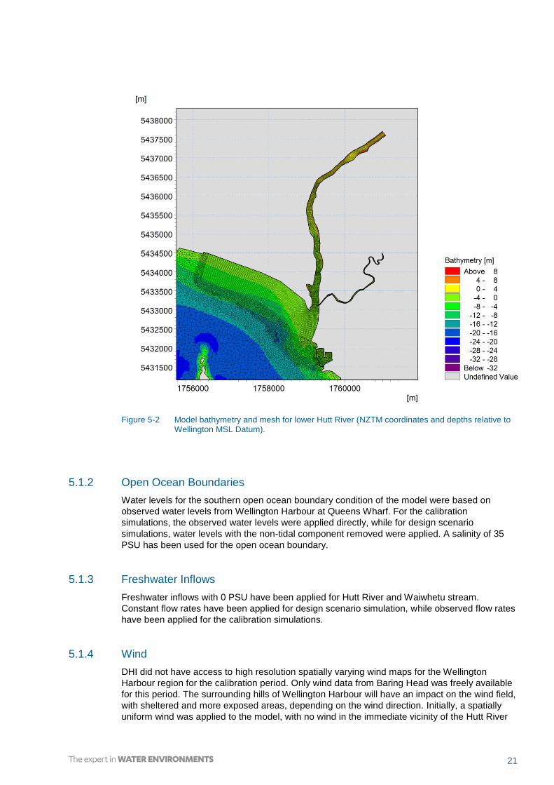
Figure 5-2 Model bathymetry and mesh for lower Hutt River (NZTM coordinates and depths relative to Wellington MSL Datum).

5.1.2 Open Ocean Boundaries

Water levels for the southern open ocean boundary condition of the model were based on

observed water levels from Wellington Harbour at Queens Wharf. For the calibration

simulations, the observed water levels were applied directly, while for design scenario

simulations, water levels with the non-tidal component removed were applied. A salinity of 35

PSU has been used for the open ocean boundary.

5.1.3 Freshwater Inflows

Freshwater inflows with 0 PSU have been applied for Hutt River and Waiwhetu stream.

Constant flow rates have been applied for design scenario simulation, while observed flow rates

have been applied for the calibration simulations.

5.1.4 Wind

DHI did not have access to high resolution spatially varying wind maps for the Wellington

Harbour region for the calibration period. Only wind data from Baring Head was freely available

for this period. The surrounding hills of Wellington Harbour will have an impact on the wind field,

with sheltered and more exposed areas, depending on the wind direction. Initially, a spatially

uniform wind was applied to the model, with no wind in the immediate vicinity of the Hutt River


mouth. However this created inaccurate eddies within the river mouth. To ensure that the

momentum of the river plume exiting the river was accurately modelled a constant negative v-

velocity wind was applied instead of zero in the immediate vicinity of the Hutt River entrance.

For design scenarios, spatial wind fields were applied in the same way.

5.1.5 Wastewater Representation

To simulate the behaviour of the wastewater plume the advection-dispersion (AD) module was

used. The AD module simulates the spread of dissolved and suspended substances subject to

the transport process described by the HD module. The wastewater plume was defined as a

conservative tracer (i.e. no decay rate).

5.2 Calibration

The model was deemed suitability calibrated to meet the objectives of the study. Calibration was

achieved with the following key specifications, with details of the calibration provided in sections

below:

5 vertical equidistant sigma layers to -2.5 m and 4 z levels layers below this with

thickness of 1 m, 3, 5 and 10 m respectively.

Density assumed as a function of salinity only.

Resistance length: 0.05 m.

Wind friction factor: 0.001255

Horizontal eddy viscosity: Smagorinsky formulation, constant 0.28.

Vertical eddy viscosity: log law formulation

Horizontal and vertical dispersion turned off.

5.2.1 Water Levels and Currents

Generally there was a good agreement between observed and predicted water levels for the

whole calibration period (15th May to 7th July 2013). This is illustrated through the comparison of

observed and predicted water levels at Estuary Bridge on Hutt River for the period 2nd to 15th

June 2013, presented in Figure 5-3.

23

Figure 5-3 Comparison of observed and predicted water levels for Hutt River at Estuary Bridge for period 2nd to 15th June 2013.

Currents were available from ADCPs within the Hutt River and mid Harbour. Both data sets

have some inherent issues as discussed below.

The location of the mid harbour ADCP was selected since, for the previous NIWA assessment,

one of the potential outfall locations was 2 km south of Somes Island. This is no longer a

potential option. Ideally an ADCP would have been located within the harbour closer to river

mouth, to illustrate the model can reasonably reproduce currents where the Hutt River enters

the Harbour. However the mid harbour ADCP was the only source of current data to calibrate

the harbour model.

The Hutt River ADCP data was not useful for calibration, since as outlined in NIWA (2013), the

ADCP was located in a back eddy which resulted in net flow upstream (i.e. positive depth

averaged north-south orientated v–velocities) for typical river flow conditions. The formation of

this eddy will be very dependent on the detailed local lower river bathymetry at the time of

measurements which are not well represented in the model. The DHI model predicts a net flow

out into the harbour (i.e. negative v-velocities) as would be expected.

The issue with the ADCP location is further illustrated if you compare surface v-velocity with

wind speed at Baring Head, as shown in Figure 5-4. Even for periods with very little wind speed,

there are periods of surface water flowing upstream for every tidal cycle (apart from when

elevated flows in river). This is not representative of general flow behaviour for the river. Stantec

(2016) undertook a dye test for Hutt River, where dye was released into surface waters on the

incoming tide at Outfall B location, with moderate north-westerly winds. The dye was observed

to still flow downstream out of the harbour mouth into the harbour, indicating no surface waters

flowing upstream.


Figure 5-4 Surface v-velcoity current from River ADCP compared with Baring Head wind speed. A positive v-velcoity corresponds to upstream flow.

The mid harbour ADCP data provided by NIWA was not post processed and there are obviously

periods with spikes of erroneous data that typically occur when the observation bin (height

above the instrument) is actually out of the water. An example of this issue is provided in Figure

5-5. This figure shows v-velocities that have been passed through a low pass filter to remove

high frequency noise for top and third from top bin against water levels at Queens Wharf in

Wellington Harbour. There is an obvious peak in current velocity as water levels drop pre and

post low tide. It is our opinion that these velocities are erroneous as currents speeds up to

0.5 m/s are unlikely to occur at this location, especially approaching low water.

Figure 5-5 Example of v velocity from bins close to surface, from mid harbour ADCP, plotted with water levels at Wellington Harbour at Queens Wharf.

A comparison of predicted u and v current velocities has only been undertaken for the top

portion of the water column for the mid harbour data, since this is the only area where the

wastewater plume will be located. The model performance for the deeper parts of the harbour

25

(i.e. depth greater than -3 m) have not been assessed since any plume concentrations at depth

will be negligible. The observed and predicted u and v velocities have been compared for the

period 1st to 17th June 2013 at approximately -0.5 m Wellington Datum as presented in Figure

5-6. At times this depth will be close to be the water surface or at a water depth of 1.5 m.

The corresponding wind behaviour at Baring Head is also presented for the corresponding

period. The odd spike due to the bin being exposed above the water surface is still apparent

however. In general there is a reasonable agreement, especially for the v-velocity component,

where can be considered the dominant velocity direction. There were a number of events where

wind speeds greater than 10 m/s. As expected for a northerly event, both observed and

predicted v velocities are negative (heading in a southerly direction) and, while for a southerly

event, both observed and predicted v velocities are positive.

In order to evaluate the performance of the calibrated model, different statistical indices were

calculated to verify the accuracy of the model results. In order to evaluate the performance of

the model, different statistical indices were computed to verify the accuracy of the model results.

The following statistical parameters have been evaluated as suggested by Ji (2008):

Mean Absolute Error (MAE):

N

n nn POabsN

MAE1

)(1

Root Mean Square Error (RMS):

2

1)(1

N

n nn PON

RMS

Relative Root Mean Square Error (RRE):

100minmax

OO

RMSRRE

where:

N = number of observation - prediction pairs

On = the value of the nth observed data

Pn = the value of the nth predicted data

Omax = maximum value of observations


Omin = minimum value of observations

The MAE indicates the average deviation between model predictions and the observed data but

does not give an indication of over prediction or under prediction. The RMS error is the average

of the squared differences between observed and predicted values and is more widely used to

assess model performance as it gives higher weightings to larger observation-prediction

differences. It is also useful to give the difference in observed and predicted values as a

percentage to measure performance. The RRE is often used for hydrodynamic modelling and is

the ratio of the RMS error to the observed change.

A summary of the calculated statistics of the model agreement with observed data is presented

in Table 5-1. The statistical analysis supported the visual interpretation of the model calibration.

Table 5-1 Summary of calibration statistical analysis.

Location Parameter Statistical Performance Parameter

MAE RMS RRE

Estuary Bridge Water Level (m) 0.05 0.07 3.13

NIWA Harbour

Mooring

U Velocity (m/s) 0.05 0.06 16.8

V Velocity (m/s) 0.06 0.07 13.7

27

Figure 5-6 Comparison of surface observed and predicted u (top) and v (middle) velocities mid harbour for period 1st to 17th June 2013. Corresponding wind data from Baring Head also presented (bottom).


5.2.2 Salt Wedge and River Plume

To assess the performance of the model in reproducing the behaviour of the saline intrusion and

river plume, a visual comparison was made between the observed and predicted salinities. The

aim of the calibration was not to obtain a perfect match between observed and predicted

salinities, but instead to replicate the general behaviour.

A comparison of the observed and predicted salinities is presented in Figure 5-7 and Figure 5-8.

Note that some liberty was taken for location of salinity extraction beyond 3,000 m (i.e.

difference of up to 500m in east-west direction). The reason for this is that the behaviour of the

plume will be very influenced by wind field for this area, which is not well resolved within the

model. It should also be noted that it is typically extremely difficult to resolve sharp freshwater

and saltwater interfaces in 3D models such as MIKE 3 FM. Any type of numerical dispersion

which is inherent in this type of model breaks down the buoyancy effect of the surface

freshwater (which maintains the freshwater layer), resulting in mixing across the vertical layers.

For this reason the focus is on re-producing overall thickness and general behaviour of river

plume layer, in this case considered to be for salinities less than 30 PSU.

Visually there is a sufficient agreement between the observed and predicted salinity distribution

for the river and river mouth. The model does appear to under predict the maximum extent

upstream of the salt wedge, however this was not the main focus of the model. The predicted

river plume is slightly thicker than suggested by the salinity data collected during southerly wind

events on 12th and 14th of June, however this is not unexpected with the wind data that was

available for Wellington Harbour.

29

Figure 5-7 Comparison of measured salinity profiles (left) with predicted salinity profiles (right) from 7/06/2013 14:25; 12/06/2013 08:03; 12/06/2013 10:05; and 14/06/2013 07:47.


Figure 5-8 Comparison of measured salinity profiles (left) with predicted salinity profiles (right) from 14/06/2013 9:29; 14/06/2013 10:55; 9/07/2013 14:08; and 9/07/2013 16:06.

31

6 Near-Field Assessment

This section describes the near-field modelling that was carried out using the CORMIX

modelling system. The near-field modelling provides predictions of the behaviour and dilution of

the wastewater plume in the near-field mixing zone.

Due to the constrained channel cross section and large wastewater discharge compared with

the flow of Waiwhetu Stream (a ratio of almost 2:1 for the “dry weather” scenarios and 1:1 for

“wet weather” scenarios), realistic wastewater behaviour predictions could not be obtained with

CORMIX for outfall Option A. Very little dilution of wastewater will occur within Waiwhetu Stream

and the far-field model is sufficient to predict dilutions beyond the confluence with Hutt River.

6.1 Wastewater Properties and Outfall Arrangement

As per the previous studies (DHI, 2011 and 2016), the wastewater is assumed to be freshwater

(i.e. salinity = 0 PSU), as are the river inflows.

The previous studies (DHI 2011 and 2016) illustrated that the temperature difference between

summer and winter has a negligible effect on the initial mixing of the wastewater plume,

therefore density differences between the treated wastewater effluent and receiving water are

thus represented in terms of salinity alone. Therefore, it was assumed that the wastewater

discharge temperature will be equal to the receiving water temperature.

The following outfall arrangement is associated with each location:

Option B, a horizontally discharging 1.6 m diameter pipe at approximately -0.485 m

(Wellington Datum 1953) or Mean Low Water Spring, protruding 20 m out from the left

river bank at an angle of 40° from the river bank.

Option C, a horizontally discharging 1.6 m diameter pipe on the seabed with two duckbill

valve 900 mm diameter ports, discharging vertically, with a port height 1.4 m above the

sea bed, 100 m from the left river bank.

6.2 Receiving Water Conditions

6.2.1 Receiving Water Level, Flow and Salinity

Water level, flow and salinity conditions at the potential outfall locations B and C, for the different

tide and weather conditions were determined from the far-field model.

With agreement from Stantec, for dry weather conditions approximate mean flows were selected

as constant boundary conditions for Hutt River and Waiwhetu Stream (25 m3/s and 0.3 m3/s

respectively). For wet weather conditions a constant flow of 100 m3/s and 2 m3/s were used for

Hutt River and Waiwhetu Stream, also with agreement from Stantec.

Water level, flow and salinity predictions for the two outfall locations and scenarios are outlined

in Table 6-1. Salinity stratification was incorporated in CORMIX by having a density jump at the

depth of the indicated salt wedge interface, with 0 PSU above and 35 PSU assumed below this

depth.


Table 6-1 Water level, flow and salinity predictions for the different outfall locations and scenarios.

Outfall

Location Parameter

Condition

Dry Weather

High Tide

Dry Weather

Mid Ebb

Dry Weather

Low Tide

Dry Weather

Mid Flood

Wet

Weather

Low Tide

Spring Neap Spring Neap Spring Neap Spring Neap Spring

Option B

Water

Level

(m)

1.0 0.7 0.3 0.3 -0.3 -0.2 0.3 0.3 0.3

Flow

(m3/s) 25.0 25.0 55.0 45.0 25.0 25.0 -2.0 5.0 100

Salinity

Behaviour Salt wedge interface approx. -0.5 m below water surface

Salt wedge

interface

approx. -1.4

m below

water

surface

Option C

Water

Level

(m)

1.0 0.7 0.3 0.3 -0.3 -0.2 0.3 0.3 0.3

Flow

(m3/s) 25.0 25.0 50.0 40.0 25.0 25.0 -2.0 8.0 100

Salinity

Salt wedge interface approx. -0.5 m below water surface

Salt wedge

interface

approx. -1.0

m below

water

surface

6.2.2 Receiving Water Bathymetry

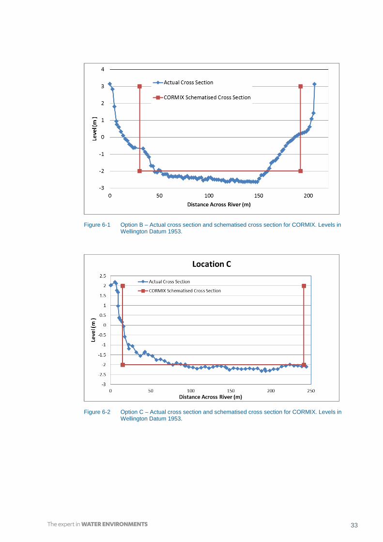
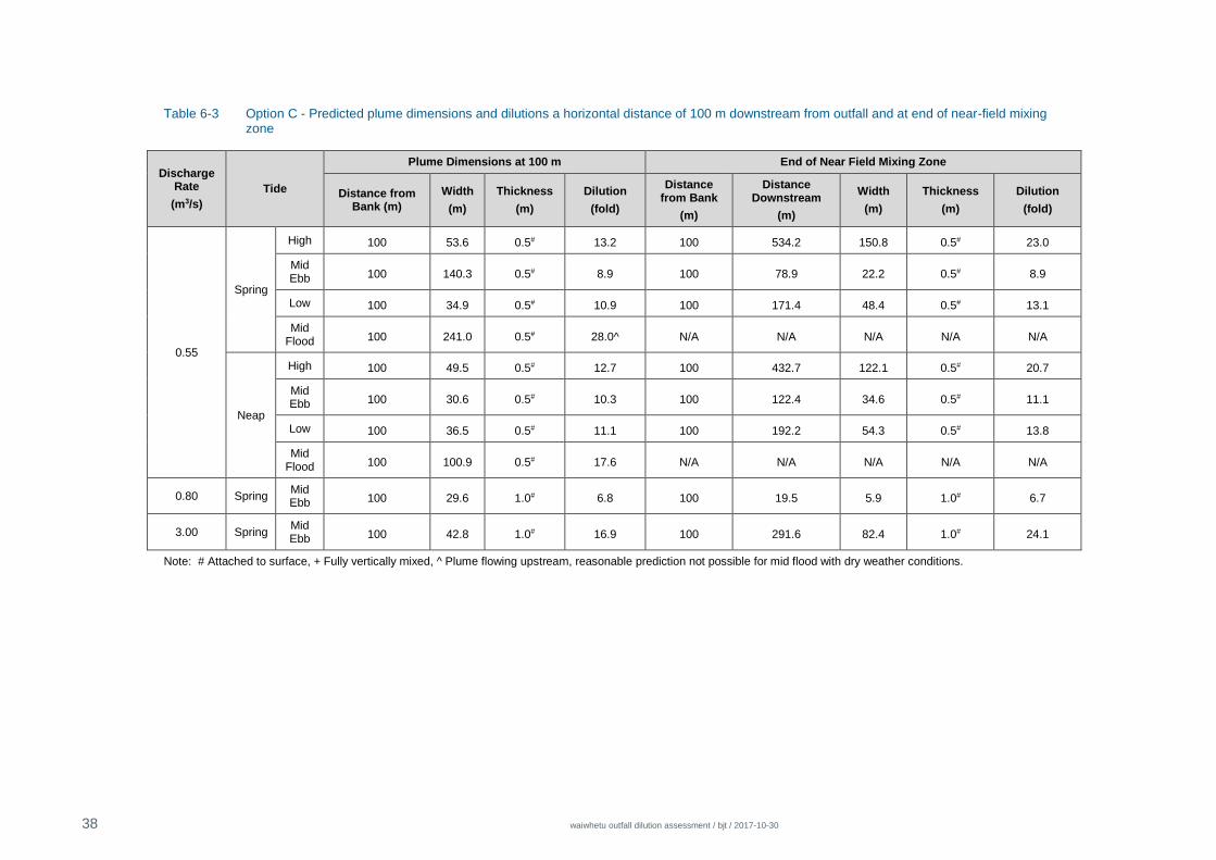
For all outfall options a cross section Manning’s n of 0.03 was applied in the CORMIX models.

Surveyed cross sections at the outfall locations for Option B and C were obtained from the

GWRC set of Hutt River cross sections.

When predicting dilutions for rivers, CORMIX assumes a rectangular cross section. Therefore

the cross sections at the location of Option B and C were schematized to an appropriate

rectangular cross section, ensuring that the schematized rectangular cross section has the

same cross sectional area as the surveyed cross section. Comparisons of the schematised

cross sections with the actual cross sections are shown in Figure 6-1 to Figure 6-2.

Option B was schematised as 162 m wide and a bed level of -2.0 m (Wellington Datum 1953).

Option C was schematised as 241 m wide and a bed level of -2.0 m (Wellington Datum 1953).

33

Figure 6-1 Option B – Actual cross section and schematised cross section for CORMIX. Levels in Wellington Datum 1953.

Figure 6-2 Option C – Actual cross section and schematised cross section for CORMIX. Levels in Wellington Datum 1953.


6.2.3 Situations where Modifications of Assumptions were Required to Obtain Dilution Predictions

Although CORMIX is on the whole a very flexible tool, there are still some criteria which must be

met before CORMIX will provide a prediction of the behaviour of the discharged wastewater. A

good example is that for submerged outfalls, the diameter of the outfall pipe must be one third or

less of the total water depth before a prediction will be provided.

For some of the scenarios and discharge locations, different assumptions were necessary either

as a result of the assumptions not meeting the required criteria of CORMIX or where predictions

were obviously erroneous. Detailed below are the situations where the CORMIX inputs or

outputs were different from the assumptions described in the sections above.

6.2.3.1 Option B Option B is essentially a surface discharge for all states of the tide, sometimes discharging

directly into the top of water column or discharging above the water surface. To ensure that the

wastewater plume would discharge into the freshwater layer overlying the salt wedge, and that

CORMIX would acknowledge the existence of the salinity stratification (i.e. if outfall invert below

freshwater layer, CORMIX unfortunately assumes no stratification), the outfall was included for

all scenarios as a 1.6 diameter pipe above the water surface. CORMIX was able to incorporate

the fact the outfall is protruding 20 m out from the left river bank at an angle of 40° from the river

bank.

6.2.3.2 Option C It was not possible to assume a two port outfall with CORMIX and similar to Option B the outfall

centre had to discharge into freshwater layer for CORMIX to acknowledge the salinity

stratification. The outfall was schematised as a 0.55 m diameter outfall (smaller than 0.9m since

the outfall dimeter must always be less than 1/3 the water depth), with the pipe centre just within

the freshwater layer. Sensitivity testing illustrated that the plume is positively buoyant and would

rise quickly to the freshwater layer. It can be assumed that the CORMIX predictions will be

conservative without this initial mixing as the plume rises through the salt wedge. CORMIX was

able to incorporate the fact the outfall is 100 m from the left river bank.

6.3 Model Results

The CORMIX model was utilised to provide predictions of the following 100 m downstream of

the discharge point and at the edge of the near-field mixing zone (see Table 6-2 and Table 6-3)

for the specified discharge and climate scenarios:

Dilution;

Plume width;

Distance from outfall; and

Plume thickness.

CORMIX provides the following advice with regard to uncertainty in the model predictions with

every model simulation results file, “extensive comparison with field and laboratory data has

shown that the CORMIX predictions on dilutions (with associated plume geometries) are reliable

for the majority of cases and are accurate to within about +-50% (standard deviation)”.

The following is a summary of the predicted dilution behaviour of the wastewater discharged

from Option B:

35

Salinity stratification for the full tidal cycle significantly decreases the dilution of wastewater,

since the wastewater plume will be very positively buoyant compared with the receiving

water which inhibits the mixing of wastewater. The wastewater will remain within the

overlying freshwater layer where it fully mixes vertically.

For the dry weather condition with a 1.1 m3/s discharge on outgoing tide, dilutions range

from 3.6 fold to 6.0 fold at a distance of 100 m from outfall and 3.1 to 8.8 fold at end of

near-field mixing zone, with a range of 12 to 350 m from the outfall.

For the wet weather conditions with a constant 0.8 m3/s discharge, a dilution of 3.3 fold is

achieved at a distance of 100 m from the outfall location and 1.8 fold at end of near-field

mixing zone 2 m downstream of the outfall.




The following is a summary of the predicted dilution behaviour of the wastewater discharged

from Option C:

Salinity stratification for the full tidal cycle significantly decreases the dilution of wastewater,

since the wastewater plume will be very positively buoyant compared with the receiving

water which inhibits the mixing of wastewater. The wastewater will remain within the

overlying freshwater layer where it fully mixes vertically.

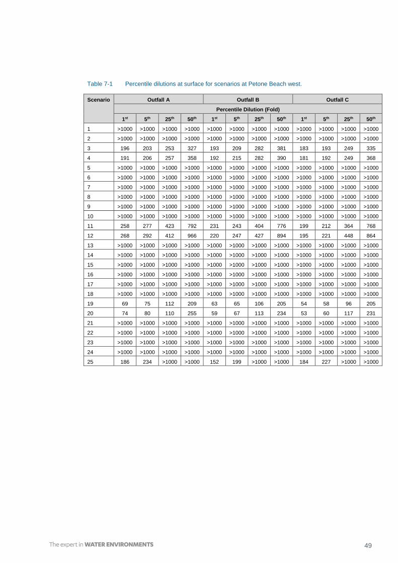
For the dry weather condition with a 0.55 m3/s discharge, dilutions range from 8.9 fold to

28.0 fold at a distance of 100 m from outfall and 8.9 to 23.0 fold at end of near-field mixing

zone, with a range of 79 to 534 m from the outfall.







The model mesh elements at Outfall B are approximately 25 m wide, while at Outfall C the mesh

elements are approximately 40 m wide. To incorporate the near-field CORMIX predictions into

the far-field model, the following logic was followed for including sources based on the plume

predictions 100 m from outfall:

Option B

For dry weather conditions – 3 sources across 65 m width, across top layer, attached to

left river bank.

For wet weather conditions and 0.8 m3/s discharge – 1 source across 7 m width, across

top layer, centred 20 m from left river bank.

For wet weather conditions and 3.0 m3/s discharge – 1 source across 19 m width,

across top layer, centred 20 m from left river bank.


Option C

For dry weather conditions – 3 sources across 86 m width, across top layer, centred

100 m from left river bank.

For wet weather conditions and 0.8 m3/s discharge – 1 source across 30 m width,


For wet weather conditions and 3.0 m3/s discharge – 1 sources across 43 m width,


37

Table 6-2 Option B - Predicted plume dimensions and dilutions a horizontal distance of 100 m downstream from outfall and at end of near-field mixing zone.

Discharge Rate

(m3/s)

Tide

Plume Dimensions at 100 m End of Near Field Mixing Zone

Distance from Bank (m)

Width

(m)

Thickness

(m)

Dilution

(fold)

Distance from Bank

(m)

Distance Downstream

(m)

Width

(m)

Thickness

(m)

Dilution

(fold)

1.10

Spring

High 70.0 16.9 0.5# 4.7 108.8 349.3 52.4 0.5# 8.5

Mid Ebb Attached to bank 74.5 0.6# 6.0 26.5 12.2 3.1 2.3+ 3.7

Low Attached to bank 91.8 0.5# 3.6 26.6 23.0 24.7 0.3# 3.1

Neap

High 66.4 16.8 0.5# 4.7 90.2 281.1 42.4 0.5# 7.7

Mid Ebb Attached to bank 83.9 0.5# 5.6 26.9 11.9 3.3 2.3+ 3.5

Low Attached to bank 106.0 0.5# 3.9 27.1 24.7 27.2 0.3# 3.3

0.80 Spring Mid Ebb 20.6 7.0 1.4# 3.3 20.6 2.0 3.9 1.4# 1.8

3.00 Spring Mid Ebb 24.7 18.6 1.4# 2.4 24.7 18.6 3.9 1.4# 2.3

Note: # Attached to surface, + Fully vertically mixed


Table 6-3 Option C - Predicted plume dimensions and dilutions a horizontal distance of 100 m downstream from outfall and at end of near-field mixing zone

Discharge Rate

(m3/s)

Tide

Plume Dimensions at 100 m End of Near Field Mixing Zone

Distance from Bank (m)

Width

(m)

Thickness

(m)

Dilution

(fold)

Distance from Bank

(m)

Distance Downstream

(m)

Width

(m)

Thickness

(m)

Dilution

(fold)

0.55

Spring

High 100 53.6 0.5# 13.2 100 534.2 150.8 0.5# 23.0

Mid Ebb 100 140.3 0.5# 8.9 100 78.9 22.2 0.5# 8.9

Low 100 34.9 0.5# 10.9 100 171.4 48.4 0.5# 13.1

Mid Flood 100 241.0 0.5# 28.0^ N/A N/A N/A N/A N/A

Neap

High 100 49.5 0.5# 12.7 100 432.7 122.1 0.5# 20.7

Mid Ebb 100 30.6 0.5# 10.3 100 122.4 34.6 0.5# 11.1

Low 100 36.5 0.5# 11.1 100 192.2 54.3 0.5# 13.8

Mid Flood 100 100.9 0.5# 17.6 N/A N/A N/A N/A N/A

0.80 Spring Mid Ebb 100 29.6 1.0# 6.8 100 19.5 5.9 1.0# 6.7

3.00 Spring Mid Ebb 100 42.8 1.0# 16.9 100 291.6 82.4 1.0# 24.1

Note: # Attached to surface, + Fully vertically mixed, ^ Plume flowing upstream, reasonable prediction not possible for mid flood with dry weather conditions.

39

7 Far-Field Assessment

This section presents the wastewater dilution predictions from the far-field model for the

selected scenarios.

7.1 Model Results

To provide an overview of the wastewater plume behaviour, plots are provided of 5th and 50th

percentile dilutions, at the surface, for selected scenarios. In this case spring tide, dry weather

conditions with calm, 90th percentile northerly and 90th percentile southerly wind conditions.

These are presented in Figure 7-1 to Figure 7-9. The percentile analysis of dilutions, covers the

duration of the discharge (5 days for dry weather and 1 day for wet weather) and two

subsequent days after the discharge finishes. For calm conditions, the wastewater plume tends

to migrate southwards towards the harbour entrance, with reasonable lateral spread across the

harbour. For southerly wind, the plume is transported northwards towards Petone beach, while

for northerly wind, the plume is very thin and closely follows the eastern shoreline out through

the harbour entrance.

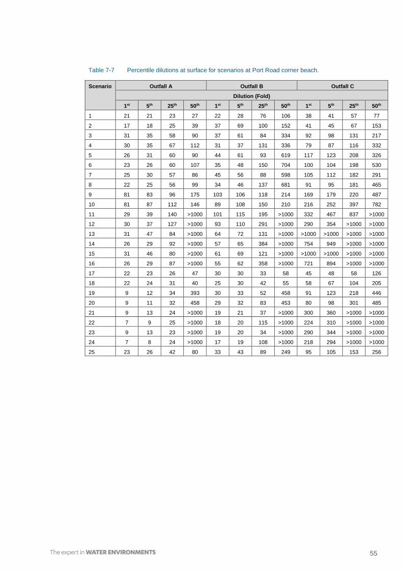
The 1st, 5th, 25th and 50th percentiles of dilutions at the surface at the sensitive sites for all

scenarios is presented in Table 7-1 to Table 7-8. The 5th and 50th percentile dilutions are the

main focus for Stantec, therefore the minimum dilutions for these percentiles for each discharge

condition are also presented in Table 7-9 to Table 7-11.

To provide an indication of the visitation frequency of the plume from each outfall at the sites,

percentile plots (see Figure 7-10 to Figure 7-16) at the sensitive sites were also generated for

the 30 day simulation (Scenario 25), which included a range of representative wind conditions

within the harbour. This illustrates the percentage of time at each site that a dilution is predicted

to be achieved. The plot for Waione Street Bridge was not included, since it is predicted the

plume will never be transported to this location for any outfall or condition. For these plots any

dilutions greater than 10,000 fold were presented as 10,000 fold.


potential outfall locations, before visitation of the plume occurred at the sensitive sites,

especially for the eastern sites. Outfall B generally performed slightly better than Outfall A,

however not for all conditions and sites.


Figure 7-1 5th percentile (top) and 50th percentile dilution (bottom), at surface, for Outfall A with dry weather conditions and calm wind condition.

41

Figure 7-2 5th percentile (top) and 50th percentile dilution (bottom), at surface, for Outfall B with dry weather conditions and calm wind condition.


Figure 7-3 5th percentile (top) and 50th percentile dilution (bottom), at surface, for Outfall C with dry weather conditions and calm wind condition.

43

Figure 7-4 5th percentile (top) and 50th percentile dilution (bottom), at surface, for Outfall A with dry weather conditions and 90th percentile southerly wind condition.


Figure 7-5 5th percentile (top) and 50th percentile dilution (bottom), at surface, for Outfall B with dry weather conditions and 90th percentile southerly wind condition.

45

Figure 7-6 5th percentile (top) and 50th percentile dilution (bottom), at surface, for Outfall C with dry weather conditions and 90th percentile southerly wind condition.


Figure 7-7 5th percentile (top) and 50th percentile dilution (bottom), at surface, for Outfall A with dry weather conditions and 90th percentile northerly wind condition.

47

Figure 7-8 5th percentile (top) and 50th percentile dilution (bottom), at surface, for Outfall B with dry weather conditions and 90th percentile northerly wind condition.


Figure 7-9 5th percentile (top) and 50th percentile dilution (bottom), at surface, for Outfall C with dry weather conditions and 90th percentile northerly wind condition.

49

Table 7-1 Percentile dilutions at surface for scenarios at Petone Beach west.

Scenario Outfall A Outfall B Outfall C

Percentile Dilution (Fold)

1st 5th 25th 50th 1st 5th 25th 50th 1st 5th 25th 50th

1 >1000 >1000 >1000 >1000 >1000 >1000 >1000 >1000 >1000 >1000 >1000 >1000

2 >1000 >1000 >1000 >1000 >1000 >1000 >1000 >1000 >1000 >1000 >1000 >1000

3 196 203 253 327 193 209 282 381 183 193 249 335

4 191 206 257 358 192 215 282 390 181 192 249 368

5 >1000 >1000 >1000 >1000 >1000 >1000 >1000 >1000 >1000 >1000 >1000 >1000

6 >1000 >1000 >1000 >1000 >1000 >1000 >1000 >1000 >1000 >1000 >1000 >1000

7 >1000 >1000 >1000 >1000 >1000 >1000 >1000 >1000 >1000 >1000 >1000 >1000

8 >1000 >1000 >1000 >1000 >1000 >1000 >1000 >1000 >1000 >1000 >1000 >1000

9 >1000 >1000 >1000 >1000 >1000 >1000 >1000 >1000 >1000 >1000 >1000 >1000

10 >1000 >1000 >1000 >1000 >1000 >1000 >1000 >1000 >1000 >1000 >1000 >1000

11 258 277 423 792 231 243 404 776 199 212 364 768

12 268 292 412 966 220 247 427 894 195 221 448 864

13 >1000 >1000 >1000 >1000 >1000 >1000 >1000 >1000 >1000 >1000 >1000 >1000

14 >1000 >1000 >1000 >1000 >1000 >1000 >1000 >1000 >1000 >1000 >1000 >1000

15 >1000 >1000 >1000 >1000 >1000 >1000 >1000 >1000 >1000 >1000 >1000 >1000

16 >1000 >1000 >1000 >1000 >1000 >1000 >1000 >1000 >1000 >1000 >1000 >1000

17 >1000 >1000 >1000 >1000 >1000 >1000 >1000 >1000 >1000 >1000 >1000 >1000

18 >1000 >1000 >1000 >1000 >1000 >1000 >1000 >1000 >1000 >1000 >1000 >1000

19 69 75 112 209 63 65 106 205 54 58 96 205

20 74 80 110 255 59 67 113 234 53 60 117 231

21 >1000 >1000 >1000 >1000 >1000 >1000 >1000 >1000 >1000 >1000 >1000 >1000

22 >1000 >1000 >1000 >1000 >1000 >1000 >1000 >1000 >1000 >1000 >1000 >1000

23 >1000 >1000 >1000 >1000 >1000 >1000 >1000 >1000 >1000 >1000 >1000 >1000

24 >1000 >1000 >1000 >1000 >1000 >1000 >1000 >1000 >1000 >1000 >1000 >1000

25 186 234 >1000 >1000 152 199 >1000 >1000 184 227 >1000 >1000


Table 7-2 Percentile dilutions at surface for scenarios at Petone Beach east.


Dilution (Fold)


1 >1000 >1000 >1000 >1000 >1000 >1000 >1000 >1000 >1000 >1000 >1000 >1000

2 >1000 >1000 >1000 >1000 >1000 >1000 >1000 >1000 >1000 >1000 >1000 >1000

3 156 166 200 243 134 144 196 269 142 148 172 209

4 145 154 209 251 132 142 198 264 141 149 180 223

5 >1000 >1000 >1000 >1000 >1000 >1000 >1000 >1000 >1000 >1000 >1000 >1000

6 >1000 >1000 >1000 >1000 >1000 >1000 >1000 >1000 >1000 >1000 >1000 >1000

7 >1000 >1000 >1000 >1000 >1000 >1000 >1000 >1000 >1000 >1000 >1000 >1000

8 >1000 >1000 >1000 >1000 >1000 >1000 >1000 >1000 >1000 >1000 >1000 >1000

9 >1000 >1000 >1000 >1000 >1000 >1000 >1000 >1000 >1000 >1000 >1000 >1000

10 >1000 >1000 >1000 >1000 >1000 >1000 >1000 >1000 >1000 >1000 >1000 >1000

11 261 323 508 >1000 245 276 431 >1000 191 207 339 866

12 273 316 566 >1000 260 296 506 934 209 220 348 746

13 >1000 >1000 >1000 >1000 >1000 >1000 >1000 >1000 >1000 >1000 >1000 >1000

14 >1000 >1000 >1000 >1000 >1000 >1000 >1000 >1000 >1000 >1000 >1000 >1000

15 >1000 >1000 >1000 >1000 >1000 >1000 >1000 >1000 >1000 >1000 >1000 >1000

16 >1000 >1000 >1000 >1000 >1000 >1000 >1000 >1000 >1000 >1000 >1000 >1000

17 >1000 >1000 >1000 >1000 >1000 >1000 >1000 >1000 >1000 >1000 >1000 >1000

18 >1000 >1000 >1000 >1000 >1000 >1000 >1000 >1000 >1000 >1000 >1000 >1000

19 71 89 138 284 65 76 116 269 53 58 93 234

20 74 87 155 284 70 80 134 248 57 61 94 200

21 >1000 >1000 >1000 >1000 >1000 >1000 >1000 >1000 >1000 >1000 >1000 >1000

22 >1000 >1000 >1000 >1000 >1000 >1000 >1000 >1000 >1000 >1000 >1000 >1000

23 >1000 >1000 >1000 >1000 >1000 >1000 >1000 >1000 >1000 >1000 >1000 >1000

24 >1000 >1000 >1000 >1000 >1000 >1000 >1000 >1000 >1000 >1000 >1000 >1000

25 211 278 >1000 >1000 169 237 >1000 >1000 208 273 >1000 >1000

51

Table 7-3 Percentile dilutions at surface for scenarios at Waione Street Bridge.


Dilution (Fold)


1 >1000 >1000 >1000 >1000 >1000 >1000 >1000 >1000 >1000 >1000 >1000 >1000

2 >1000 >1000 >1000 >1000 >1000 >1000 >1000 >1000 >1000 >1000 >1000 >1000

3 >1000 >1000 >1000 >1000 >1000 >1000 >1000 >1000 >1000 >1000 >1000 >1000

4 >1000 >1000 >1000 >1000 >1000 >1000 >1000 >1000 >1000 >1000 >1000 >1000

5 >1000 >1000 >1000 >1000 >1000 >1000 >1000 >1000 >1000 >1000 >1000 >1000

6 >1000 >1000 >1000 >1000 >1000 >1000 >1000 >1000 >1000 >1000 >1000 >1000

7 >1000 >1000 >1000 >1000 >1000 >1000 >1000 >1000 >1000 >1000 >1000 >1000

8 >1000 >1000 >1000 >1000 >1000 >1000 >1000 >1000 >1000 >1000 >1000 >1000

9 >1000 >1000 >1000 >1000 >1000 >1000 >1000 >1000 >1000 >1000 >1000 >1000

10 >1000 >1000 >1000 >1000 >1000 >1000 >1000 >1000 >1000 >1000 >1000 >1000

11 >1000 >1000 >1000 >1000 >1000 >1000 >1000 >1000 >1000 >1000 >1000 >1000

12 >1000 >1000 >1000 >1000 >1000 >1000 >1000 >1000 >1000 >1000 >1000 >1000

13 >1000 >1000 >1000 >1000 >1000 >1000 >1000 >1000 >1000 >1000 >1000 >1000

14 >1000 >1000 >1000 >1000 >1000 >1000 >1000 >1000 >1000 >1000 >1000 >1000

15 >1000 >1000 >1000 >1000 >1000 >1000 >1000 >1000 >1000 >1000 >1000 >1000

16 >1000 >1000 >1000 >1000 >1000 >1000 >1000 >1000 >1000 >1000 >1000 >1000

17 >1000 >1000 >1000 >1000 >1000 >1000 >1000 >1000 >1000 >1000 >1000 >1000

18 >1000 >1000 >1000 >1000 >1000 >1000 >1000 >1000 >1000 >1000 >1000 >1000

19 >1000 >1000 >1000 >1000 >1000 >1000 >1000 >1000 >1000 >1000 >1000 >1000

20 >1000 >1000 >1000 >1000 >1000 >1000 >1000 >1000 >1000 >1000 >1000 >1000

21 >1000 >1000 >1000 >1000 >1000 >1000 >1000 >1000 >1000 >1000 >1000 >1000

22 >1000 >1000 >1000 >1000 >1000 >1000 >1000 >1000 >1000 >1000 >1000 >1000

23 >1000 >1000 >1000 >1000 >1000 >1000 >1000 >1000 >1000 >1000 >1000 >1000

24 >1000 >1000 >1000 >1000 >1000 >1000 >1000 >1000 >1000 >1000 >1000 >1000

25 >1000 >1000 >1000 >1000 >1000 >1000 >1000 >1000 >1000 >1000 >1000 >1000


Table 7-4 Percentile dilutions at surface for scenarios at 100m downstream of Hutt/Waiwhetu confluence.


Dilution (Fold)


1 3 3 5 14 3 3 17 >1000 >1000 >1000 >1000 >1000

2 2 3 5 21 3 4 6 >1000 >1000 >1000 >1000 >1000

3 3 3 4 10 3 4 9 249 398 472 >1000 >1000

4 2 3 4 19 3 4 6 335 409 521 >1000 >1000

5 3 3 5 15 2 3 6 >1000 >1000 >1000 >1000 >1000

6 3 3 5 18 3 4 7 >1000 >1000 >1000 >1000 >1000

7 3 3 5 13 2 3 6 >1000 >1000 >1000 >1000 >1000

8 3 3 5 17 3 4 7 >1000 >1000 >1000 >1000 >1000

9 3 3 14 >1000 7 14 105 >1000 >1000 >1000 >1000 >1000

10 3 3 9 >1000 7 15 297 >1000 >1000 >1000 >1000 >1000

11 3 3 13 >1000 8 10 457 >1000 >1000 >1000 >1000 >1000

12 3 3 11 >1000 7 17 >1000 >1000 >1000 >1000 >1000 >1000

13 3 4 12 >1000 5 9 55 >1000 >1000 >1000 >1000 >1000

14 3 4 9 >1000 7 14 175 >1000 >1000 >1000 >1000 >1000

15 3 4 12 >1000 5 9 54 >1000 >1000 >1000 >1000 >1000

16 3 4 9 >1000 7 14 154 >1000 >1000 >1000 >1000 >1000

17 2 2 6 >1000 3 5 45 >1000 >1000 >1000 >1000 >1000

18 2 2 3 >1000 3 5 195 >1000 >1000 >1000 >1000 >1000

19 1 1 5 >1000 3 3 218 >1000 >1000 >1000 >1000 >1000

20 1 2 3 >1000 3 5 >1000 >1000 >1000 >1000 >1000 >1000

21 2 2 6 >1000 2 3 18 >1000 >1000 >1000 >1000 >1000

22 2 2 3 >1000 3 5 112 >1000 >1000 >1000 >1000 >1000

23 2 2 6 >1000 2 3 18 >1000 >1000 >1000 >1000 >1000

24 2 2 3 >1000 3 5 104 >1000 >1000 >1000 >1000 >1000

25 3 3 4 6 3 4 6 31 >1000 >1000 >1000 >1000

53

Table 7-5 Percentile dilutions at surface for scenarios at Lowry Bay.


Dilution (Fold)


1 58 59 63 99 67 68 77 168 93 94 102 165

2 67 69 75 116 74 76 86 124 92 99 109 158

3 65 66 77 98 54 57 71 123 94 97 113 133

4 59 60 73 102 56 58 76 118 92 94 115 142

5 >1000 >1000 >1000 >1000 >1000 >1000 >1000 >1000 >1000 >1000 >1000 >1000

6 >1000 >1000 >1000 >1000 >1000 >1000 >1000 >1000 >1000 >1000 >1000 >1000

7 >1000 >1000 >1000 >1000 >1000 >1000 >1000 >1000 >1000 >1000 >1000 >1000

8 >1000 >1000 >1000 >1000 >1000 >1000 >1000 >1000 >1000 >1000 >1000 >1000

9 94 99 117 177 115 118 135 201 159 164 200 313

10 96 103 123 224 112 119 144 314 175 184 218 576

11 71 76 109 327 75 80 112 347 142 146 214 581

12 66 72 100 279 71 76 112 317 137 139 221 543

13 >1000 >1000 >1000 >1000 >1000 >1000 >1000 >1000 >1000 >1000 >1000 >1000

14 >1000 >1000 >1000 >1000 >1000 >1000 >1000 >1000 >1000 >1000 >1000 >1000

15 >1000 >1000 >1000 >1000 >1000 >1000 >1000 >1000 >1000 >1000 >1000 >1000

16 >1000 >1000 >1000 >1000 >1000 >1000 >1000 >1000 >1000 >1000 >1000 >1000

17 26 28 33 47 33 33 38 54 43 44 54 80

18 28 30 35 62 32 34 41 88 48 50 58 154

19 21 22 31 92 21 22 31 94 39 40 57 153

20 20 21 29 80 20 21 31 87 37 38 59 148

21 >1000 >1000 >1000 >1000 >1000 >1000 >1000 >1000 >1000 >1000 >1000 >1000

22 >1000 >1000 >1000 >1000 >1000 >1000 >1000 >1000 >1000 >1000 >1000 >1000

23 >1000 >1000 >1000 >1000 >1000 >1000 >1000 >1000 >1000 >1000 >1000 >1000

24 >1000 >1000 >1000 >1000 >1000 >1000 >1000 >1000 >1000 >1000 >1000 >1000

25 94 128 377 >1000 71 134 497 >1000 126 165 548 >1000


Table 7-6 Percentile dilutions at surface for scenarios at Days Bay.


Dilution (Fold)


1 74 79 101 184 80 83 103 179 113 114 127 237

2 80 86 114 163 79 84 102 152 121 129 146 283

3 >1000 >1000 >1000 >1000 >1000 >1000 >1000 >1000 >1000 >1000 >1000 >1000

4 >1000 >1000 >1000 >1000 >1000 >1000 >1000 >1000 >1000 >1000 >1000 >1000

5 147 153 200 270 131 138 189 346 257 264 306 402

6 108 116 188 306 117 124 177 342 233 246 291 460

7 141 150 193 296 105 108 151 789 237 240 257 364

8 104 114 201 369 106 109 141 655 220 231 254 416

9 100 113 155 471 114 127 157 555 135 146 192 862

10 104 109 151 325 114 119 156 416 152 157 173 655

11 >1000 >1000 >1000 >1000 >1000 >1000 >1000 >1000 >1000 >1000 >1000 >1000

12 >1000 >1000 >1000 >1000 >1000 >1000 >1000 >1000 >1000 >1000 >1000 >1000

13 124 135 182 >1000 147 158 211 >1000 223 230 324 >1000

14 122 136 198 683 147 153 216 790 215 218 319 >1000

15 146 148 293 >1000 171 176 288 >1000 248 277 347 >1000

16 138 143 292 >1000 171 184 307 >1000 242 273 390 >1000

17 29 32 43 122 33 35 43 145 37 39 48 212

18 29 31 43 83 33 34 43 109 41 43 46 163

19 >1000 >1000 >1000 >1000 >1000 >1000 >1000 >1000 >1000 >1000 >1000 >1000

20 >1000 >1000 >1000 >1000 >1000 >1000 >1000 >1000 >1000 >1000 >1000 >1000

21 34 37 50 319 41 44 59 387 60 62 86 668

22 34 38 54 188 41 43 59 216 59 60 85 370

23 40 41 81 >1000 48 49 81 >1000 69 76 96 >1000

24 39 40 82 >1000 48 52 85 >1000 68 75 107 >1000

25 100 108 166 305 87 99 145 393 153 165 211 327

55

Table 7-7 Percentile dilutions at surface for scenarios at Port Road corner beach.


Dilution (Fold)


1 21 21 23 27 22 28 76 106 38 41 57 77

2 17 18 25 39 37 69 100 152 41 45 67 153

3 31 35 58 90 37 61 84 334 92 98 131 217

4 30 35 67 112 31 37 131 336 79 87 116 332

5 26 31 60 90 44 61 93 619 117 123 208 326

6 23 26 60 107 35 48 150 704 100 104 198 530

7 25 30 57 86 45 56 88 598 105 112 182 291

8 22 25 56 99 34 46 137 681 91 95 181 465

9 81 83 96 175 103 106 118 214 169 179 220 487

10 81 87 112 146 89 108 150 210 216 252 397 782

11 29 39 140 >1000 101 115 195 >1000 332 467 837 >1000

12 30 37 127 >1000 93 110 291 >1000 290 354 >1000 >1000

13 31 47 84 >1000 64 72 131 >1000 >1000 >1000 >1000 >1000

14 26 29 92 >1000 57 65 384 >1000 754 949 >1000 >1000

15 31 46 80 >1000 61 69 121 >1000 >1000 >1000 >1000 >1000

16 26 29 87 >1000 55 62 358 >1000 721 894 >1000 >1000

17 22 23 26 47 30 30 33 58 45 48 58 126

18 22 24 31 40 25 30 42 55 58 67 104 205

19 9 12 34 393 30 33 52 458 91 123 218 446

20 9 11 32 458 29 32 83 453 80 98 301 485

21 9 13 24 >1000 19 21 37 >1000 300 360 >1000 >1000

22 7 9 25 >1000 18 20 115 >1000 224 310 >1000 >1000

23 9 13 23 >1000 19 20 34 >1000 290 344 >1000 >1000

24 7 8 24 >1000 17 19 108 >1000 218 294 >1000 >1000

25 23 26 42 80 33 43 89 249 95 105 153 256


Table 7-8 Percentile dilutions at surface for scenarios at Seaview Marina.


Dilution (Fold)


1 26 29 37 48 67 70 79 124 62 69 83 91

2 32 36 48 61 74 82 111 144 73 77 89 106

3 36 39 49 61 36 37 45 283 76 78 88 104

4 30 34 49 73 37 38 43 277 74 76 86 109

5 34 36 49 56 35 36 43 626 98 99 105 172

6 26 30 48 70 39 40 49 568 98 100 105 197

7 34 35 48 55 34 35 41 600 94 95 101 159

8 26 30 47 68 38 38 47 555 96 97 103 187

9 82 83 98 208 100 104 121 251 156 175 201 434

10 79 84 131 176 110 116 169 235 196 204 312 606

11 29 33 61 >1000 54 56 62 >1000 152 162 217 >1000

12 27 35 58 >1000 53 55 67 >1000 131 156 245 >1000

13 36 45 57 >1000 56 57 78 >1000 260 271 776 >1000

14 34 38 58 >1000 52 55 111 >1000 245 263 >1000 >1000

15 36 44 56 >1000 54 56 75 >1000 250 259 747 >1000

16 34 37 57 >1000 50 53 106 >1000 235 254 >1000 >1000

17 23 24 27 56 29 30 34 69 42 47 54 112

18 22 24 36 48 31 33 46 62 53 55 80 154

19 9 10 17 571 15 16 17 574 42 45 58 653

20 9 10 17 553 15 15 19 626 38 45 67 693

21 10 13 17 >1000 16 17 22 >1000 79 84 221 >1000

22 10 10 17 >1000 15 16 33 >1000 74 83 349 >1000

23 10 13 17 >1000 16 17 21 >1000 76 80 214 >1000

24 10 10 17 >1000 15 16 31 >1000 72 80 337 >1000

25 26 30 42 53 35 37 42 97 81 89 100 119

57

Table 7-9 Minimum 5th and 50th percentile dilutions for dry weather simulations for sensitive sites for each outfall.

Sensitive Site Outfall A Outfall B Outfall C

5th 50th 5th 50th 5th 50th

Petone Beach west 203 327 199 381 192 335

Petone Beach east 154 243 142 264 148 209

Waione Street Bridge >1000 >1000 >1000 >1000 >1000 >1000

100m downstream of

Hutt/Waiwhetu confluence 3 6 3 31 472 >1000

Lowry Bay 59 98 57 118 94 133

Days Bay 79 163 83 152 114 237

Port Road corner beach 18 27 28 106 41 77

Seaview Marina 29 48 35 97 69 91

Table 7-10 Minimum 5th and 50th percentile dilutions for wet weather simulations (0.8 m3/s discharge) for sensitive sites for each outfall.




Petone Beach east 316 >1000 276 934 207 746


100m downstream of

Hutt/Waiwhetu confluence 3 >1000 9 >1000 >1000 >1000

Lowry Bay 72 47 76 201 139 313

Days Bay 109 83 119 416 146 655


Seaview Marina 33 48 53 235 156 434

Table 7-11 Minimum 5th and 50th percentile dilutions for wet weather simulations (3.0 m3/s discharge) for sensitive sites for each outfall.




Petone Beach east 87 284 76 248 58 200


100m downstream of

Hutt/Waiwhetu confluence 1 >1000 3 >1000 >1000 >1000

Lowry Bay 21 47 21 54 38 80

Days Bay 31 83 34 109 39 163


Seaview Marina 10 48 15 62 45 112


Figure 7-10 Percentile plot of dilutions at Petone Beach west for Scenario 25.

Figure 7-11 Percentile plot of dilutions at Petone Beach east for Scenario 25.

59

Figure 7-12 Percentile plot of dilutions at 100m downstream of Hutt/Waiwhetu confluence for Scenario 25. Note logarithmic scale.

Figure 7-13 Percentile plot of dilutions at Lowry Bay for Scenario 25. Note logarithmic scale.


Figure 7-14 Percentile plot of dilutions at Days Bay for Scenario 25. Note logarithmic scale.

Figure 7-15 Percentile plot of dilutions at Port Road corner beach for Scenario 25. Note logarithmic scale.

61

Figure 7-16 Percentile plot of dilutions at Seaview Marina for Scenario 25. Note logarithmic scale.


8 Summary

Stantec commissioned DHI to undertake a plume dispersion study for the existing wastewater

overflow from Seawater Wastewater Treatment Plant into Waiwhetu Stream and for two

potential alternative wastewater overflows, to form part of an AEE. The three locations for which

the assessment was undertaken were:


Option B - Hutt River (near Waiwhetu Stream mouth) close to the water surface;


The potential scenarios for overflow discharge were as follows:

typical dry weather discharge rate of 0.55 m3/s (1.10 m3/s for Option B on outgoing tide)

for a duration of 5 days;

typical dry weather discharge rate of 0.55 m3/s (1.10 m3/s for Option B on outgoing tide)

for a duration of 30 days;

wet weather discharge rate of 0.8 m3/s for a duration of 1 day; and

wet weather discharge rate of 3.0 m3/s for a duration of 1 day.

The discharged wastewater plumes will mix and dilute due to two types of mixing processes;

near-field mixing (driven by buoyancy and momentum of discharged plume) and far-field mixing

(driven conditions in the surrounding water i.e. currents).

Near-field dilution predictions were undertaken with the empirically based model CORMIX, while

far-field dilution predictions were carried out with the fully dynamic 3D model, MIKE 3 FM. The

two models were indirectly coupled, with the near-field model providing the general initial

conditions for the wastewater plume within the 3D model. The salt wedge which propagates up

the lower Hutt River will have an influence on the mixing of the discharged wastewater, therefore

it was important that this behaviour was reasonably reproduced by the 3D model.

The 3D model was calibrated using data collected specifically for the study by NIWA, in

conjunction with data obtained from GWRC. Generally there was a good agreement between

observed and predicted water levels within the river mouth and there was a reasonable

agreement between observed and predicted current speeds within the harbour at the water

surface. There was also a sufficient agreement between the observed and predicted salinity

distribution for the river and river mouth.

Near-field dilution predictions were calculated for Outfall B and Outfall C for a range of tidal and

wastewater discharge conditions. Near-field dilution predictions were not possible for Outfall A,

since the discharge rates were of the same order as the stream flow. For Outfall B and C,

salinity stratification during the full tidal cycle significantly decreases the dilution of wastewater,

since the wastewater plume will be very positively buoyant compared with the receiving water

which inhibits the mixing of wastewater. The wastewater will remain within the overlying

freshwater layer (after rising from the sea bed for Outfall C), where it fully mixes vertically.

The performance of each outfall location was assessed by determining the far-field plume

dilution that will occur for a range of selected discharge, hydrodynamic and climate scenarios (a

total of 25 scenarios) at sensitive sites within the river mouth and harbour. Both neap and spring

tidal conditions were considered, along with calm, southerly and northerly wind conditions.

Predicted 1st, 5th, 25th and 50th percentile dilutions at the sensitive sites were calculated for each

scenario and outfall location. Spatial maps of the predicted 5th and 50th percentile dilutions for

63

each outfall, were also presented for selected scenarios to provide an overview of the

wastewater plume behaviour for different types of wind conditions. For calm conditions, the

wastewater plume tends to migrate southwards towards the harbour entrance, with reasonable

lateral spread across the harbour. For southerly wind the plume is transported northwards

towards Petone beach, while for northerly wind, the plume is very thin and closely follows the

eastern shoreline out through the harbour entrance.

Percentile plots at the sensitive sites were also generated for the 30 day simulation which

included a range of representative wind conditions within the harbour.


potential outfall locations, before visitation of the plume occurred at the sensitive sites,

especially for the eastern sites. Outfall B generally performed better than Outfall A, however not

for all conditions and sites.


9 References

Ahrens, C. (2003); Meteorology Today: An introduction to Weather, Climate and the

Environment. Brooks/Cole

DHI (2011); Hutt River / Wellington: Preliminary Wastewater Dilution Assessment. Report

prepared for HCC.

DHI (2016); Waiwhetu Outfall – CORMIX Modelling Two Additional Options. Technical memo

prepared for HCC.

DHI (2017); MIKE 3 Flow Model FM, Hydrodynamic Module, User Guide.

Doneker, R.L and G.H Jirka (2007); CORMIX User Manual: A Hydrodynamic Mixing Zone Model

and Decision Support System for Pollutant Discharges into Surface Waters. U.S Environment

Protection Agency.

Heath (1977); Circulation and hydrography of Wellington Harbour. New Zealand Oceanographic

Institute oceanographic summary 12.

NIWA (2013); HCC Plume Dispersal: Data Report. Report prepared for MWH NZ Ltd. on behalf

of Hutt City Council, September 2013.

NIWA (2015); HCC Plume Dispersal: Summary Report. Report prepared for MWH NZ Ltd. on

behalf of Hutt City Council, March 2015.

Stantec (2016); Flood tide flows from the Hutt River to the Waiwhetu Stream Memorandum.

Documents

Waiwhetu Outfall Dilution Assessment