Wage regulation and the quality of police officer recruits

IFS Working Paper W15/19

Rowena CrawfordRichard Disney

The Institute for Fiscal Studies (IFS) is an independent research institute whose remit is to carry out rigorous economic research into public policy and to disseminate the findings of this research. IFS receives generous support from the Economic and Social Research Council, in particular via the ESRC Centre for the Microeconomic Analysis of Public Policy (CPP). The content of our working papers is the work of their authors and does not necessarily represent the views of IFS research staff or affiliates.

1

Wage regulation and the quality of police officer recruits

June 2015

Rowena Crawford Richard Disney*

Institute for Fiscal Studies Institute for Fiscal Studies

University College, London

University of Sussex

Abstract

The paper analyses the impact of centrally regulated pay on the quality of applicants

to be police officers in England and Wales using a unique dataset of individual test

scores from the national assessment that is required of all applicants. It provides

empirical evidence of two distinct channels through which centrally regulated pay

induces variation in the quality of applicants. First, national wage setting implies that

relative wages between the police and other occupations vary spatially. We show that

higher outside wages are associated with lower quality applicants, using several

spatially-varying measures of outside wages. Second, nationally-set wages cannot

adjust to reflect spatial variation in the disamenity of an occupation. We demonstrate

that a greater disamenity of policing (as measured primarily by area differences in

crime rates and in the proportion of crime that is violent) is also associated with lower

quality police applicants.

JEL: J31 J38

Keywords: Police pay Wage regulation Workforce quality

Acknowledgement

This research has been funded by the Economic and Social Research Council through grant ES L008

165/1 to the Institute for Fiscal Studies for the project ‘Economics of the police: recruitment, retention and

finance’. The College of Policing, CIPFA and the Home Office are thanked for making specific police data

available to us; no conclusions drawn here should be attributable to those organisations. The work also

utilises data from the Annual Survey of Hours and Earnings and the New Earnings Survey Panel

Dataset, produced by the Office for National Statistics and supplied by the Secure Data Service at the

UK Data Archive. Labour Force Survey data were also utilised, supplied through the UK Data Archive.

These data are Crown Copyright and reproduced with the permission of the controller of HMSO and

Queen’s Printer for Scotland. We should thank audiences at presentations to the Home Office, the

College of Policing, the Institute for Fiscal Studies and the University of Sussex for helpful comments.

*Corresponding author. Email: richard_d@ifs.org.uk. Address: Institute for Fiscal Studies, 7

Ridgmount Street, London, WC1E 7AE, UK. Tel: +44 207 291 4800.

2

1. Introduction

Pay rates for public sector workers throughout most of Europe and parts of the United

States are centrally negotiated and heavily regulated: for example, by applying

common scale rates across local employers. This can have a number of important

implications. First, national wage setting often leads to spatial variation in public

sector pay differentials relative to private sector outside options. Second, national

wage setting means that wages cannot adjust to reflect spatial differences in the

disamenity of working in a public sector occupation. These facts lead to the natural

inferences that (all else equal) in areas where regulated public sector pay is low

relative to private sector pay, or in areas where the disamenity of the public sector

occupation is high, public sector workers are of lower quality (and vice versa).

In this paper we utilise a unique dataset to analyse the impact of centrally regulated

pay on the quality of a particular group of public sector workers: the police in

England and Wales. Our paper is the first to our knowledge to consider

simultaneously both the aforementioned channels through which national wages may

affect quality, and we provide empirical evidence in support of both relative wages

and the disamenity of policing affecting the quality of applicants to the local police

force. Furthermore, the novel data that we use – individual test scores from the

national assessment required of all applicants – provide a direct measure of ‘quality’

pertinent to the occupation in question, and therefore represents an improvement over

the existing literature that has relied on inference from prior schooling or institutional

performance.

Our work brings together two strands of the existing literature. First, our paper

augments studies which confirm the proposition of Borjas (2002) that lower pay of

public sector workers relative to outside options lowers the supply and worsens the

quality of employees in the public sector. A number of studies, notably Nickell and

Quintini (2002) in the United Kingdom and Hoxby and Leigh (2004) and Bacolod

(2007) in the United States, use pre-entry educational test scores as measures of

ability and show that temporal and/or spatial variations in public pay relative to

private pay affect public sector recruitment. In similar vein, a recent paper by Dal Bó,

Finan and Rossi (2013) utilises an interesting public sector recruitment drive with a

degree of randomisation of pay offers to show that higher public sector wages and

3

better job attributes attract higher quality workers to the public sector, as measured by

IQ, personality and aptitude tests. The implications of differential worker quality on

public sector performance have been noted in some studies. Propper and Van Reenen

(2010) suggest that spatial variations in mortality rates across public hospitals in the

UK’s National Health Service can be linked to differences in worker quality arising

from these relative pay disparities and therefore indirectly to centralised pay

regulation.1 Propper and Britton (2012) obtain the same result in terms of regulation

of the pay of public school teachers and school performance in England, with similar

findings on teachers in the United States by Hanushek et al (2004).

Second, our paper builds on the literature on compensating variation and wage

differentials. In the standard approach, in competitive labour markets wage

differentials in part compensate for the non-pecuniary (dis)advantages of a particular

occupation (Rosen, 1986) and for the (dis)advantages of locating and working in a

particular geographical area (Roback, 1982, 1988). Where wages are centrally

regulated, such compensating adjustments do not occur (at least, overtly) and the

quality and composition of the workforce is thereby affected by these (dis)advantages.

Although in some public sector occupations, variation in non-pecuniary

characteristics within the occupation may be relatively limited, there is some evidence

of this variation being a factor in the supply of workers to public health care (Di

Tommaso, Strom, and Saether 2009) and it is most certainly true that, for example,

inner city policing is a very different form of police activity from policing a largely

rural area. Hence, we expect local variations in the nature of policing to play a

significant role in spatial differences in recruit type and quality in the police service

when wages are centrally regulated.

The police labour market has been studied much less in recent years than other public

sector occupations such as teachers and workers in health professions

(notwithstanding the contribution of Mas (2006) on decentralised pay arbitration

awards to police officers in the United States). It should be noted that, unlike in the

United States, pay of police officers in England and Wales is broadly set within a

national framework, with little variation in pay (at least, outside London). To set the

1 This finding may also reflect spatial differences in management quality since the outcome measures

apply to the hospital as a whole: see Bloom et al (2010).

4

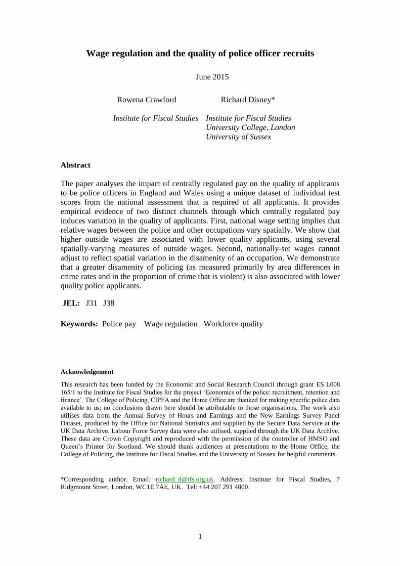
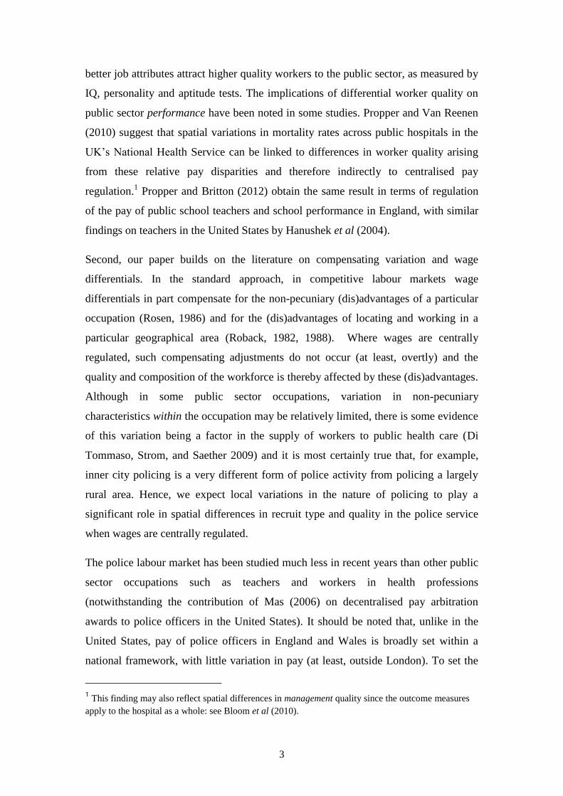
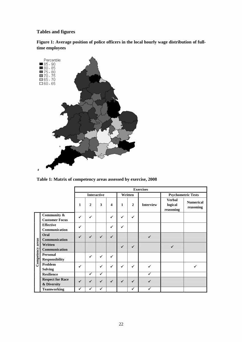
scene Figure 1 illustrates the geographical variation in police relative wages resulting

from centralised wage-setting, mapping the average position of junior police officers

in the local hourly wage distribution for the 43 police forces of England and Wales.

Not surprisingly, junior police officers lie at a higher percentile of the hourly wage

distribution in predominantly rural police force areas and are significant lower in the

wage distribution in the relatively affluent areas around London.

The paper now proceeds as follows. In section 2 we describe the police recruitment

process in England and Wales. In section 3 we introduce a simple theoretical model,

which produces some testable implications of the impact of national wage setting on

applicant quality. In section 4 we describe our empirical approach and the data used,

while section 5 presents our results. Section 6 concludes.

2. Institutional context

Law enforcement in England and Wales is undertaken by police officers attached to

43 territorial police forces operating at the county or metropolitan level.2 There is not

the ‘layering’ of federal, state and local police forces found in the United States,

although there are now some specialist national agencies including the National

Crime Agency. Pay levels are set through national negotiating procedures and are

broadly uniform across forces, although officers in London receive a flat ‘London

weighting allowance’ worth from 5-10% of pay by pay grade.3

The police recruitment process in England and Wales has several stages. It can be

summarised as follows (see also HMSO, 2012, pp.76-88 and 661-673). Would-be

police officers apply to their local police force, which operates a screening process to

sift out unsuitable candidates such as those who fail basic standards of physical and

financial fitness, have a criminal record etc. This first stage can be somewhat ad hoc.

HMSO (2012) (‘The Winsor Review’) noted:

“Candidates must apply to a police force using a standard application form.

Given the number of potential applicants, forces will generally apply a practical

sift of potential applicants before deciding those who are to be given an

2 Scotland and Northern Ireland each have a unified police force.

3 For further discussion of the police remuneration structure, see HMSO (2011) and Crawford and

Disney (2014).

5

application form as a first stage in the recruitment process. This can involve

requiring potential applicants to attend a familiarisation event… Other forces

may simply limit the number of forms that are printed… [One force] had a

small number of police vacancies, and decided to limit the number of printed

application forms to 500. The first 500 people who telephoned the force on an

appointed day received the forms…” (ibid, p.77)

In addition to filling out the application form, some forces may also require a certain

level of minimum educational achievement (such as a qualification at A-level

equivalent) and set other, additional criteria, such as possession of a clean driving

licence. The application form contains a competency-based questionnaire which must

be filled in to a satisfactory standard.

Candidates who achieve this standard in the questionnaire are then submitted to the

national recruitment assessment process, administered by the National Policing

Improvement Agency (NPIA) between 2006 and 2012 and subsequently by the

newly-established College of Policing. Known as SEARCH (Structured Entrance

Assessment for Recruiting Constables Holistically), this assessment process aims to

gauge candidates’ performance in seven competency areas through a combination of

interactive role play, written exercises, tests of verbal, numerical and logical

reasoning, and an interview.4 Each candidate is given a score for each competency

area, as well as an overall score and an indication of whether he or she has passed or

failed.

Pass rates have varied over time since the SEARCH process was introduced and have

tended to increase as forces improve their strategy in selecting applicants for

submission (since the submission of an applicant incurs a direct financial cost for

individual police forces), and because information on the assessment tests (including

worked examples to actual questions) has begun to be published on websites and in

hard copy. However, as we shall see, pass rates vary significantly across candidates

4 The seven competency areas assessed are: Community and Customer Focus, Effective

Communication, Personal Responsibility, Problem Solving, Resilience, Respect for Race and Diversity

and Teamworking. Effective communication is further broken down into Oral Communication and

Written Communication.

6

submitted by individual police forces and pass scores have also been changed from

time to time.

A candidate who obtains at least a pass score may then be appointed to the police

force which submitted him or her. If there is a surplus of successful candidates, a

force can require a higher test score than the national pass mark or use some other

non-discriminatory selection criterion, but it cannot hire below the pass mark – hence,

if a police force lacks successful candidates, it may be able to recruit from successful

applicants submitted by another force who either choose not to join that force or who,

despite passing, were not hired by the force that submitted them to the assessment.

Despite this possibility of joining a different force, it should be emphasised that the

vast majority of successful candidates accept a job offer from the police force that

submitted them for assessment (though they may in subsequent years move to another

force). Overall, from 2006 to 2011, the pass rate was over 60%, and 97% of those

who passed found a job as a police officer. Once employed as a police officer, the

individual is placed on the national pay scale, with subsequent pay enhancements

related to tenure, additional skill enhancements and promotion.

3. Theoretical model

Here we set out a simple model is to illustrate why a nationally regulated wage for

police officers can result in spatial variation in the quality of police applicants.

Consider an economy with two regions, , in which there are region specific

prices and respectively, and (potentially) region specific wages. In each region

there are two occupations, , where is the superscript for policing and

the superscript for all other occupations. The labour market for policing is regulated in

that there is a nationally set wage ( ), while the labour market for other occupations

is unregulated and wages potentially vary between the two regions.

Workers come in many skill types, . ‘Skill’ in this specific context should be

interpreted as an aptitude for police work. This aptitude depends not just on

observable characteristics (such as education and experience) but also potentially on

characteristics that are not just unobserved to the researcher but which may also be

unobserved to the sponsoring police force and to the applicant themselves, as

illustrated by the fact that some candidates fail to achieve the required standard in the

national assessment.

7

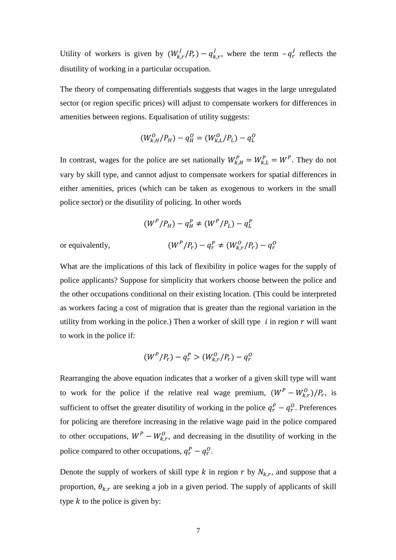
Utility of workers is given by

, where the term –

reflects the

disutility of working in a particular occupation.

The theory of compensating differentials suggests that wages in the large unregulated

sector (or region specific prices) will adjust to compensate workers for differences in

amenities between regions. Equalisation of utility suggests:

In contrast, wages for the police are set nationally

. They do not

vary by skill type, and cannot adjust to compensate workers for spatial differences in

either amenities, prices (which can be taken as exogenous to workers in the small

police sector) or the disutility of policing. In other words

or equivalently,

What are the implications of this lack of flexibility in police wages for the supply of

police applicants? Suppose for simplicity that workers choose between the police and

the other occupations conditional on their existing location. (This could be interpreted

as workers facing a cost of migration that is greater than the regional variation in the

utility from working in the police.) Then a worker of skill type in region will want

to work in the police if:

Rearranging the above equation indicates that a worker of a given skill type will want

to work for the police if the relative real wage premium, , is

sufficient to offset the greater disutility of working in the police

. Preferences

for policing are therefore increasing in the relative wage paid in the police compared

to other occupations, , and decreasing in the disutility of working in the

police compared to other occupations,

.

Denote the supply of workers of skill type in region by , and suppose that a

proportion, are seeking a job in a given period. The supply of applicants of skill

type to the police is given by:

8

The total supply of applicants is given by and the effective supply of

potential recruits is given by where is the probability of a skill

type passing the national assessment.

Under the natural assumption that wages in the unregulated sector are increasing in

skill type, this simple model yields a number of testable implications for spatial

variations in the quality of police applicants. The quality of police applicants will be

greater in regions where:

- the relative real wage paid in the police compared to other occupations is

higher;

- the disamenity of working in the police compared to other occupations is

lower;

- there is a greater supply of better quality workers;

- the probability that workers are job seeking is higher;

The first two of these in particular arise as implications of wage regulation in the

police sector, and we provide empirical evidence in support of these propositions in

the remainder of this paper.

4. Empirical strategy and data

Our empirical approach for considering the role of local wage conditions and spatial

variation in the disamenity of policing on the quality of police applicants is based on

data for over 41,000 applicants who were submitted to the police recruitment national

assessment in the period 2007-10.5

Consider the simple equation:

Where Si is the average quality of an individual police applicant as measured by their

score in the national assessment; is the local police wage;

is the local outside

5 Few candidates were submitted in the two years after 2010 due to cuts in spending on the police as

part of the then-Coalition government’s austerity programme.

9

wage they could obtain, is the local disamenity of policing, Xr is a vector of other

local area controls and is a set of time dummies. The implications of the simple

theoretical model previously described are that and should be negative. Given that

police salary scales are set nationally, and the salary scale for officers of a given rank

are relatively short, there should be little spatial variation in the police wage and

should collapse to a constant. However, we test the sensitivity of our results to

this assumption in Section 5.

We consider two further extensions of the model. The first is where we additionally

control for a vector of individual characteristics, in the above equation. We

interpret these measured characteristics (such as age, education and type of previous

experience) as observable indicators of skill type, k, as in our economic model.

Hence, whether applicant scores are associated with local wage conditions and the

disamenity of policing then depends on the extent to which any previously identified

relationship arises from attracting (or dissuading) applicants with certain observable

characteristics that are associated with higher quality, as opposed to arising from

attracting (or dissuading) applicants with unobservable quality.

The second extension is straightforward: we directly examine the likelihood that

candidates with certain observable characteristics apply to the national assessment as

a function of spatial variation in the outside wage and the disamenity of policing.

Since there is considerable spatial variation in the characteristics of applicants, this

specification provides further evidence on the determinants of the quality of

applicants.

4.1. The quality of police applicants

Our measure of the quality of police officers is applicants’ scores from the SEARCH

national assessment. For candidates who undertook the SEARCH assessment between

2007 and 2010 we know which police force put them forward for assessment, and

have data on their overall score, and their scores for three particular competency

areas: oral communication, written communication and respect for race and diversity

(RfRD). We also have data on characteristics of the candidates (age, education,

ethnicity, previous employment, prior experience in the police). We use these both to

explore the relationship between observable characteristics and applicant quality, and

10

to examine the channels through which spatial variation in relative wages and the

disutility of policing affect the average quality of candidates.

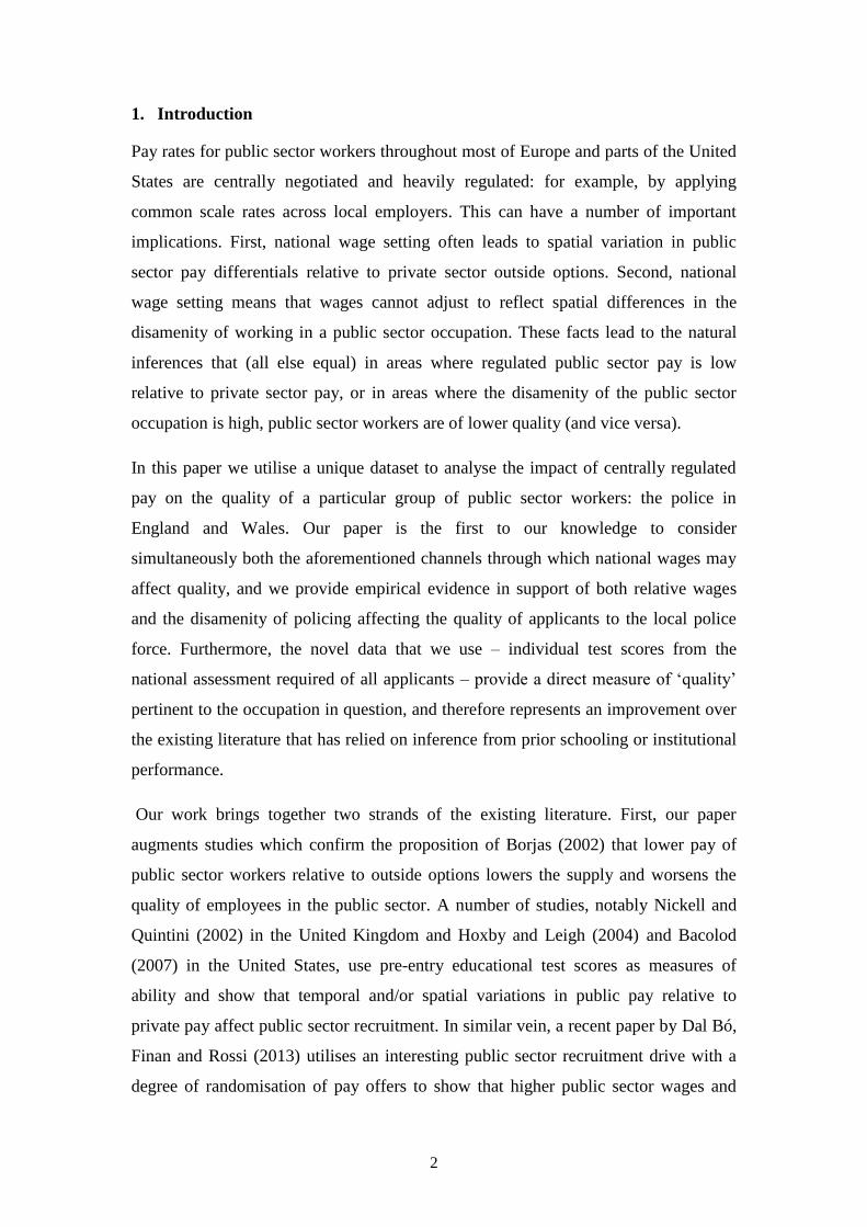
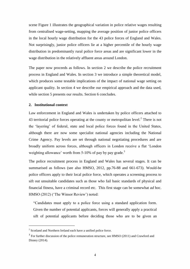
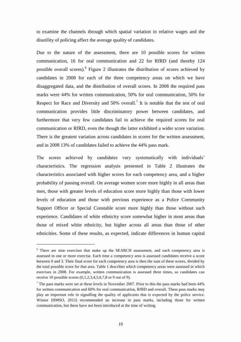
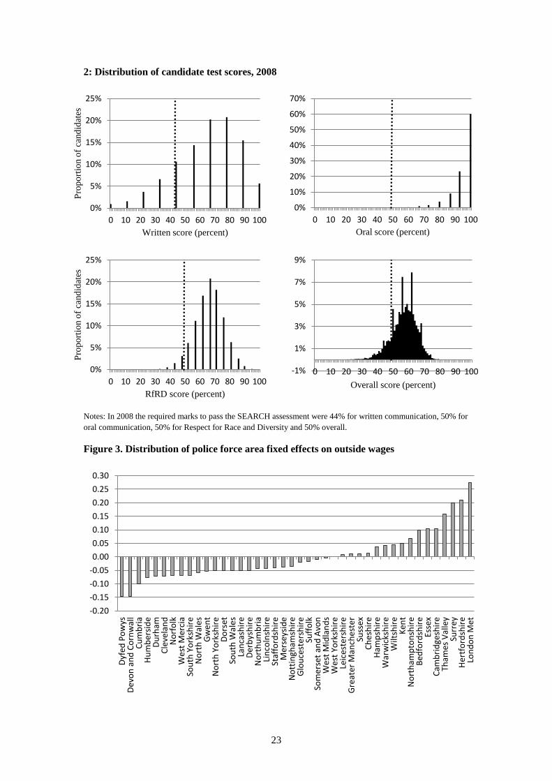
Due to the nature of the assessment, there are 10 possible scores for written

communication, 16 for oral communication and 22 for RfRD (and thereby 124

possible overall scores).6 Figure 2 illustrates the distribution of scores achieved by

candidates in 2008 for each of the three competency areas on which we have

disaggregated data, and the distribution of overall scores. In 2008 the required pass

marks were 44% for written communication, 50% for oral communication, 50% for

Respect for Race and Diversity and 50% overall.7 It is notable that the test of oral

communication provides little discriminatory power between candidates, and

furthermore that very few candidates fail to achieve the required scores for oral

communication or RfRD, even the though the latter exhibited a wider score variation.

There is the greatest variation across candidates in scores for the written assessment,

and in 2008 13% of candidates failed to achieve the 44% pass mark.

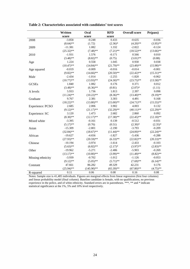
The scores achieved by candidates vary systematically with individuals’

characteristics. The regression analysis presented in Table 2 illustrates the

characteristics associated with higher scores for each competency area, and a higher

probability of passing overall. On average women score more highly in all areas than

men, those with greater levels of education score more highly than those with lower

levels of education and those with previous experience as a Police Community

Support Officer or Special Constable score more highly than those without such

experience. Candidates of white ethnicity score somewhat higher in most areas than

those of mixed white ethnicity, but higher across all areas than those of other

ethnicities. Some of these results, as expected, indicate differences in human capital

6 There are nine exercises that make up the SEARCH assessment, and each competency area is

assessed in one or more exercise. Each time a competency area is assessed candidates receive a score

between 0 and 3. Their final score for each competency area is then the sum of these scores, divided by

the total possible score for that area. Table 1 describes which competency areas were assessed in which

exercises in 2008. For example, written communication is assessed three times, so candidates can

receive 10 possible scores (0,1,2,3,4,5,6,7,8 or 9 out of 9).

7 The pass marks were set at these levels in November 2007. Prior to this the pass marks had been 44%

for written communication and 60% for oral communication, RfRD and overall. These pass marks may

play an important role in signalling the quality of applicants that is expected by the police service.

Winsor (HMSO, 2012) recommended an increase in pass marks, including those for written

communication, but these have not been introduced at the time of writing.

11

across applicants, other results clearly reflect the applicant self-selection implicit in

our theoretical model.

4.2. Estimating police wages and outside wages

While our empirical approach to wage variation has much in common with past

studies that have explored the relationship between relative pay and workforce

quality, our treatment of wages and

differs somewhat. Since we are

measuring the quality of police applicants, many of whom are young adults at the

start of their working lives, we typically do not observe an outside contemporaneous

wage for these individuals.8 Furthermore, it is not clear that it is necessarily starting

salaries that motivate career choice, or whether applicants are more forward looking.

We therefore suppose that applicants base their career choice on how wages in the

police compare to the average wages of all employees in their local area, after

controlling for employee demographic characteristics.

More formally, we estimate:

where is the wage received by an employee, is a vector of individual

characteristics and is a set of police force area dummies. The estimated value of

is an indicator of the local area fixed effect on the average outside wage, which

can be used for in our estimation of above. Note that since these

coefficients are themselves estimated, we bootstrap the two-stage process in order to

produce appropriate standard errors around our estimates in the second stage

estimation of .

We estimate in our baseline estimates using data from the Labour Force Survey

(LFS). This is a quarterly household survey, with a rotating panel element in which

households are interviewed for five successive quarters. The LFS data contain

information on individuals’ earnings (which is elicited in two of the five quarters),

and demographic information on which we can condition wages. The data do not

8 In any event, we do not of course simultaneously observe an ‘inside’ and ‘outside’ wage for any

individual. Identification strategies in the context of estimating public sector wage ‘premia’ or

‘penalties’ are discussed at some length in Disney and Gosling (2003).

12

contain identifiers for the police force area in which an individual lives, but do

contain local area identifiers which can be roughly aggregated up to police force

areas. We pool LFS data from 2005 to 2010, and estimate controlling for sex, age,

age squared, education, ethnicity, interactions between the quadratic in age and

education, and time dummies.

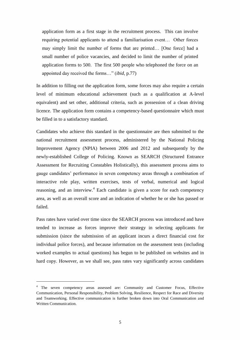
The distribution of estimated area fixed effects is illustrated in Figure 3, normalized

by subtracting the unweighted mean of . Unsurprisingly, outside wages are

estimated to be highest in London, and many of the surrounding police force areas

(Hertfordshire, Surrey and Thames Valley). In contrast, outside wages are lowest in

predominantly rural areas such as Dyfed Powys and Devon and Cornwall.

We cannot test the sensitivity of our results to the assumption that there is no spatial

variation in average police wages (conditional on observable characteristics) using the

LFS data, since the sample sizes of observed police officers is too small. However we

can use an alternative data source, the Annual Survey of Hours and Earnings, to shed

some light on this. ASHE is an employer survey that collects panel data on the

earnings and hours worked of a 1 per cent sample of employees in Great Britain.

Using pooled ASHE data from 2006 to 2009 we estimate both the previous equation

for log wages, and the expanded equation:

where is the wage received by an employee, is a vector of individual

characteristics, is a set of police force area dummies, is a dummy for whether the

employee is a police officer, and is a set of interaction terms. In both cases the

individual characteristics controlled for are simply sex, age and age squared, since

these are the only demographic characteristics available in the ASHE data. In Section

5 we test the sensitivity of our main results to the assumption that there is no spatial

variation in the police wage by controlling for the relative wage

, using

, rather than just controlling for the outside wage using .

4.3. Disamenity of policing

One of our main contributions in this paper is that we explore the relationship

between relative pay and workforce quality while simultaneously allowing for spatial

13

variation in the disamenity of policing. The indicators of disamenity that we control

for are the crime rate (number of reported crimes per 1000 population), and

composition of reported crime (the proportion of crime accounted for by 11

encompassing categories: theft, criminal damage and arson, domestic burglary, non-

domestic burglary, public order offences, shoplifting, vehicle crime, violence without

injury, violence with injury and other). We anticipate that a higher crime rate, and a

greater proportion of crime being accounted for by violence with or without injury,

would imply a greater disamenity of policing than a lower crime rate and a greater

proportion of crime being accounted for by ‘softer’ forms of crime.

These variables are constructed from data on reported crime published by the Home

Office, and population figures collated by the Chartered Institute of Public Finance

and Accountancy. The level and composition of reported crime vary annually, and the

variables are lagged one year, on the basis that individuals’ decision to apply to the

police force is most likely affected by recent observation of the level and composition

of crime.

4.4. Other controls

In all our specifications to estimate we include a dummy for London, since there

is a cost of living adjustment made to the wage of police officers in London. We also

include time dummies to control for time trends in the quality of the national

workforce (or apparent quality, if over time candidates learn how to ‘game’ the

assessment), and annual variation in the difficulty of the national assessment (the

exact exercises involved typically change annually).

Other controls for local area characteristics are also important to reduce concerns that

there are unobservable area characteristics that make it more likely that higher or

lower quality individuals would apply to the police in a given area (i.e. selection

effects). We include controls for the local unemployment rate, and the availability of

skilled labour in the local area, as measured by the proportion of the local population

aged 25-55 (inclusive) who have a degree, the proportion whose highest qualification

is A-levels (or equivalent) and the proportion whose highest qualification is below

GCSEs (or equivalent). These time-varying local area controls are estimated using the

LFS.

14

The theoretical model presented in Section 3 also predicted that higher quality

individuals would apply to the police in a given area if living costs were lower (since

then a given wage premium for working in the police would result in a greater

increase in purchasing power). A lack of suitable data means that we are unable to

control for local area differences in the general level of prices (let alone the price of a

basket of goods that police applicants may on average purchase). However, we can

include as a control the local area average house price, as an indicator of spatial

variation in the general level of prices. We construct a measure of police force area

average house price using Land Registry data on median house prices by local

authority area, and aggregating these to police force areas by weighting according to

the geographical distribution of households in the LFS. It should however be noted

that, insofar as house prices also capture spatial differences in local amenity values,

the association between house prices and police quality cannot be signed a priori.9

5. Results

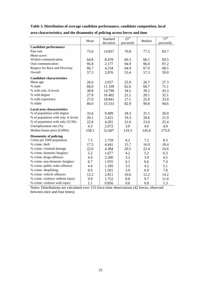
Table 3 describes the distribution of pass rates and average (mean) candidate scores

across police forces and time. There is considerable variation in pass rates: on one

quarter of occasions the annual pass rate was less than 70.8%, while on one quarter of

occasions the annual pass rate was more than 83.7%. Underlying this, there is

variation in the average scores achieved by a force’s candidates for oral

communication, written communication, respect for race and diversity, and overall.

The largest variation in average scores achieved is for written communication, as

might be expected given this was the competency area with the largest variation in

scores across candidates (shown in Figure 2).

The demographic composition of candidates put forward for assessment also differs

across forces, and this could drive some of the differences in the average scores

achieved by candidates (given that, as described in Table 2, some individual

characteristics are associated with higher scores). Variation in the composition of

candidates is summarised in Table 3. There is relatively little variation in the average

age of candidates put forward by forces. In contrast, the proportion of candidates who

were men varies from less than 62.6% for one quarter of forces’ annual submissions,

9 For a survey, see Gibbons and Machin (2008).

15

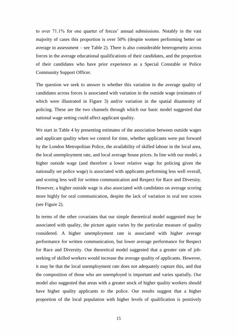
to over 71.1% for one quarter of forces’ annual submissions. Notably in the vast

majority of cases this proportion is over 50% (despite women performing better on

average in assessment – see Table 2). There is also considerable heterogeneity across

forces in the average educational qualifications of their candidates, and the proportion

of their candidates who have prior experience as a Special Constable or Police

Community Support Officer.

The question we seek to answer is whether this variation in the average quality of

candidates across forces is associated with variation in the outside wage (estimates of

which were illustrated in Figure 3) and/or variation in the spatial disamenity of

policing. These are the two channels through which our basic model suggested that

national wage setting could affect applicant quality.

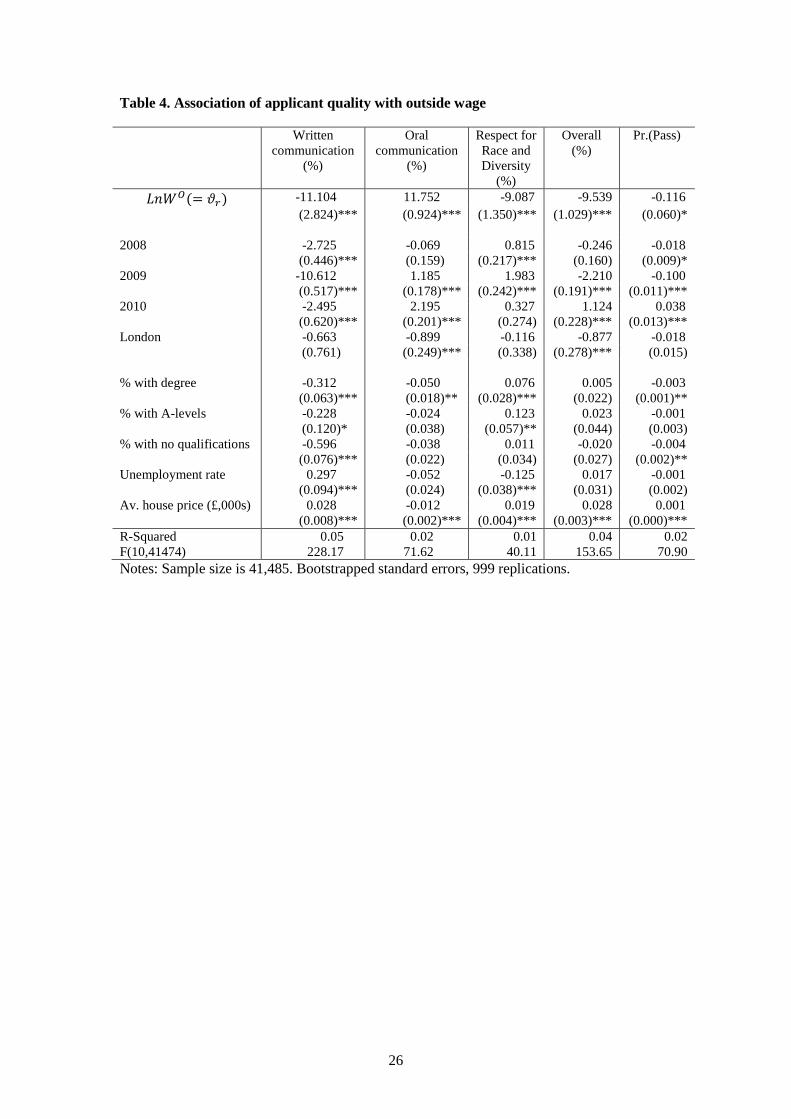
We start in Table 4 by presenting estimates of the association between outside wages

and applicant quality when we control for time, whether applicants were put forward

by the London Metropolitan Police, the availability of skilled labour in the local area,

the local unemployment rate, and local average house prices. In line with our model, a

higher outside wage (and therefore a lower relative wage for policing given the

nationally set police wage) is associated with applicants performing less well overall,

and scoring less well for written communication and Respect for Race and Diversity.

However, a higher outside wage is also associated with candidates on average scoring

more highly for oral communication, despite the lack of variation in oral test scores

(see Figure 2).

In terms of the other covariates that our simple theoretical model suggested may be

associated with quality, the picture again varies by the particular measure of quality

considered. A higher unemployment rate is associated with higher average

performance for written communication, but lower average performance for Respect

for Race and Diversity. Our theoretical model suggested that a greater rate of job-

seeking of skilled workers would increase the average quality of applicants. However,

it may be that the local unemployment rate does not adequately capture this, and that

the composition of those who are unemployed is important and varies spatially. Our

model also suggested that areas with a greater stock of higher quality workers should

have higher quality applicants to the police. Our results suggest that a higher

proportion of the local population with higher levels of qualification is positively

16

associated with average applicant for Respect for Race and Diversity, but is

negatively associated with average scores for oral communication and written

communication.

House prices are found to have a positive association with scores for written

communication and Respect for Race and Diversity, and overall scores, but a negative

association with oral communication. This result is perhaps surprising, since all else

equal a higher local price level would mean that a given wage premium for working

in the police would imply lower additional purchasing power, and therefore might be

expected to have a negative impact on the quality of applicants. However, house

prices are an imperfect measure of local differences in the cost of living, and, as

mentioned previously, could be indicative of other aspects – for example, areas with

higher house prices might be more pleasant, have lower crime rates and be easier to

police, and so have a lower disamenity of policing than other areas.

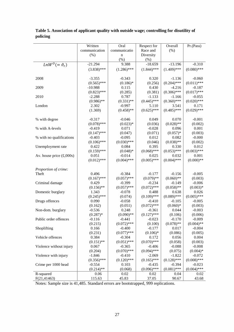
Once we control for spatial (and time) variation in our anticipated indicators of the

disutility of policing our results are strengthened in the predicted direction. This is

illustrated in Table 5. We now find a larger negative association between outside

wages and average applicant scores for written communication and respect for race

and diversity, average overall scores, and the pass rate. There remains the

unexpectedly positive association between outside wages and average scores for oral

communication, however it is worth reiterating that there is the least variation in

candidate scores (and in forces’ average candidate score) for oral communication.

Turning to the association between applicant quality and the disamenity of policing

itself, for all measures of quality the indicators of disamenity are jointly significant

using standard F-tests. We find that a higher level of crime in the local area in the year

prior to application is associated with lower average applicant scores for written

communication and respect for race and diversity, lower average overall scores, and a

lower pass rate. This would be consistent with our prior that a higher crime rate is a

disamenity of policing that would (all else equal) deter higher quality individuals.

Similarly, we find that a higher proportion of crime being accounted for by violent

crime (with or without injury) is associated with lower quality applicants on all

measures.

17

These results therefore provide broad empirical support for the main predictions of

our simple model: applicant quality is negatively associated with higher outside

wages (which, given a nationally set police wage, imply a lower relative wage for

policing), and is negatively associated with the disamenity of policing (which also

cannot be compensated for given the national wage structure).

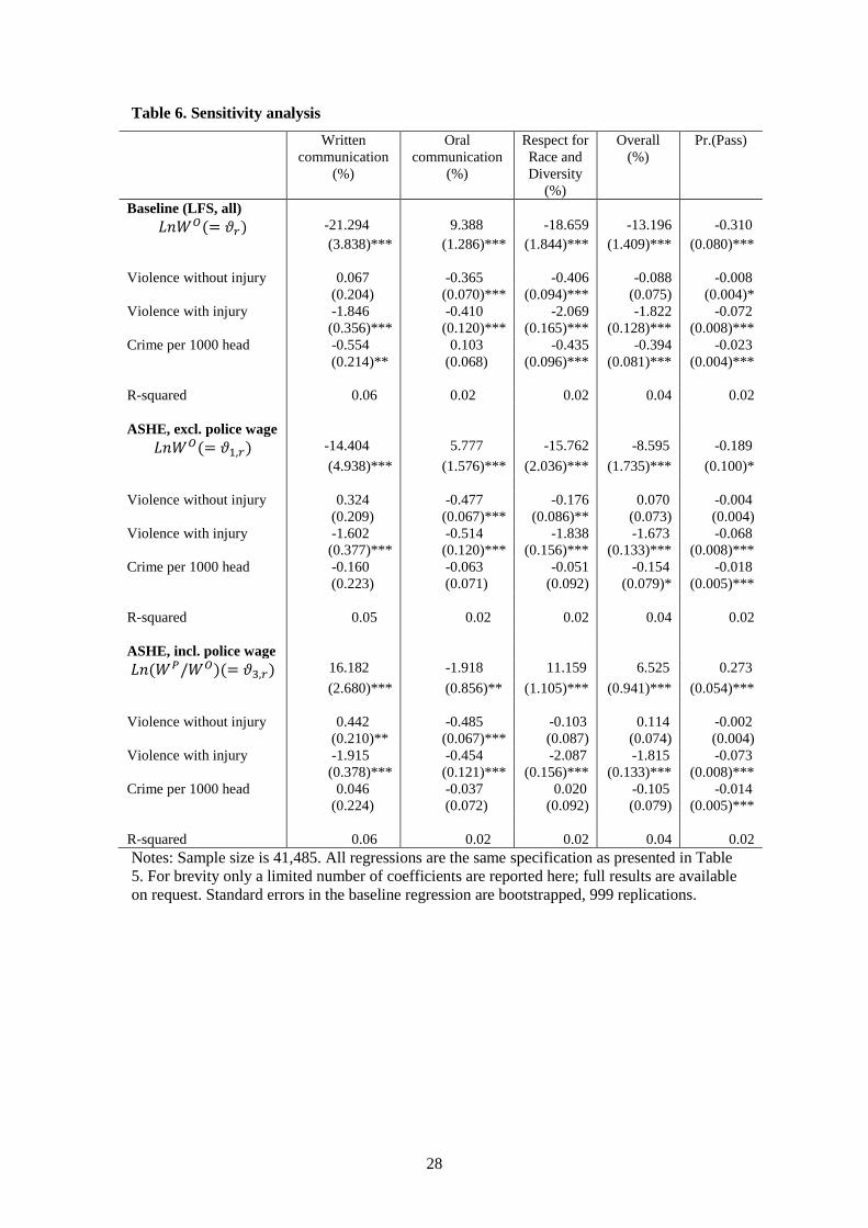
Throughout this analysis we have assumed that police wages do not vary nationally,

and therefore that spatial variation in the relative wage for the policing is completely

reflected in spatial variation in the outside wage. In Table 6 we test the sensitivity of

our results to this assumption. First, we illustrate how our results are affected by using

as our measure of outside wages the fixed effects estimated from the ASHE data.

Note that these differ from those estimated using the LFS (used throughout the rest of

the analysis in this paper) not just because the data source is different, but also

because with the ASHE data we can estimate the spatial variation in wages

conditional on age and sex only. This yields results that are qualitatively similar, but

quantitatively slightly smaller, than our main results.

Second, we illustrate how our results are affected by controlling for the local relative

wage rather than just the outside wage. This addresses the potential concern that

police wages, as opposed to scale rates, are not completely national – for example,

that higher wages could be paid by forces ‘over-promoting’ its officers up the pay

scale in areas where recruitment or retention is made more difficult by higher outside

wages. The results are shown in the bottom panel of Table 6; note that we would now

expect the sign on the relative wage to be opposite to the sign on the outside wage,

since a higher outside wage implies a lower relative wage (for a given police wage).

The results are broadly in line with those estimated just using the outside wage,

suggesting that our main results are not affected by our assumption that (conditional)

police wages do not vary spatially.

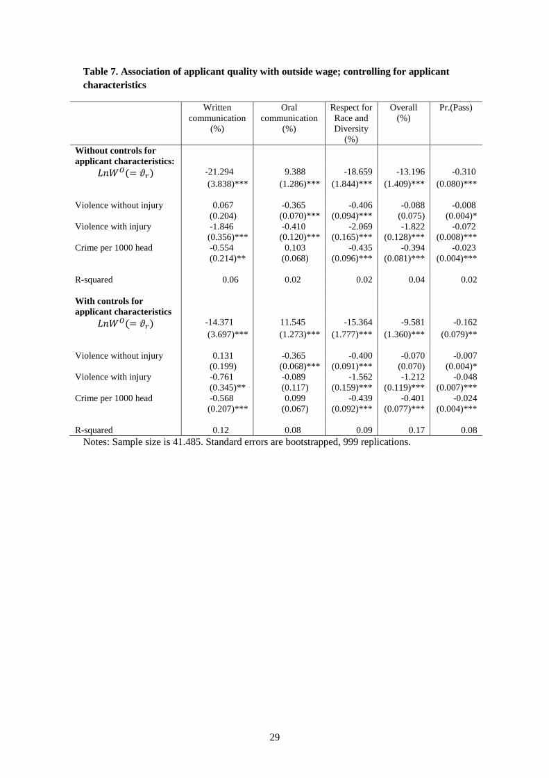
Finally, we turn to a brief discussion of how the association of quality with outside

wages and the disamenity of policing manifests itself – in particular, whether it is

driven by candidates with particular characteristics (observed skill types) being more

or less likely to apply. Table 7 illustrates the impact on our headline results from

Table 5 if we additionally control for candidate characteristics (age, sex, education,

ethnicity and previous experience as a Special Constable or a Police Community

18

Support Officer). Doing so reduces the magnitude of the associations between quality

and outside wages, and quality and disamenity, but does not eliminate them. This

suggests that part of the effect of national wages is to influence the composition of

applicants in terms of their observable characteristics, but in large part the effect

comes through differences in unobservable quality of candidates.

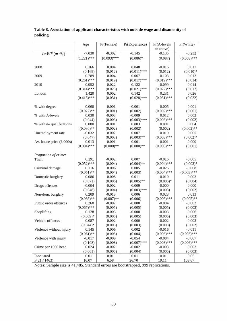
Table 8 presents the results of regressions that explore the association of candidate

characteristics (mean age, and the probability of being female, having A-levels or

higher qualifications, being of white ethnicity, and having previous policing

experience) with outside wages and the disamenity of policing. These suggest that

higher outside wages (i.e. a lower relative wage for policing) are associated with a

lower average age, and a smaller proportion of applicants who are female and who are

of white ethnicity. These are all characteristics that are associated with higher test

scores (see Table 2). There is little association between the outside wage and the

probability that an applicant has previous policing experience. However, variation in

the prevalence of previous experience among applicants is likely to be driven by

different forces’ decisions regarding the role of Special Constables and Police

Community Support Officers in their workforce, rather than a selection effect of

whether individuals with such experience go on to apply to be police officers. There is

also little association between broad measures of the educational qualifications of

candidates and outside wages. This may reflect selection issues. In terms of the

impact of the disamenity of policing on candidate characteristics, perhaps surprisingly

we do not find that a high proportion of violent crime is association with a lower

proportion of female applicants. However, we do find that it is associated with a lower

proportion of white applicants, and a lower proportion of applicants with higher

qualifications.10

6. Conclusions

In this paper we have used a novel dataset to analyse the impact of centrally regulated

pay on the quality of applicants to the police in England and Wales. This data –

10 An interesting question is whether the nature of policing is endogenous to types of crime – for

example, as to whether police are armed (which is not automatic in the UK) and in the nature of

patrolling: see Southwick (1998) for a discussion in the US context. However we would not expect

applicants to be aware of these differences across police forces.

19

individual test scores from the national assessment required of all applicants –

provides a direct measure of ‘quality’ pertinent to the occupation in question, are

therefore represents an improvement over the existing literature that has relied on

inference from prior schooling or institutional performance.

We provide empirical evidence of two distinct channels through which centrally

regulated pay affects workforce quality. First, central wage setting implies relative

wages between the police and other occupations vary spatially and we demonstrate

that higher outside wages is associated with lower quality applicants (as measured by

their test scores). Second, national police wages cannot adjust to reflect spatial

variation in the disamenity of policing, and we demonstrate that a greater disamenity

of policing (as measured by crime rates and the proportion of crime that is violence) is

also associated with lower quality police applicants. For the most part these impacts

on applicant quality are not explained by an effect on the composition of applicants in

terms of observable characteristics. However, higher outside wages do appear to

slightly deter applications from women, older individuals, white individuals and those

with higher levels of education (all characteristics that are positively associated with

test performance), while higher disamenity of policing appears to deter older

applicants and those with higher levels of qualifications.

In the context of the police in England and Wales, the impacts on quality of spatial

variation in relative wages and spatial variation in the disamenity of policing offset

each other somewhat: the association between outside wages and quality is weaker

when disamenity is not separately controlled for. Whether this arises because the

higher relative wage in some areas directly compensates those who would otherwise

be put off by the greater disamenity of policing in those areas, or whether there are

different ‘types’ of people – those who respond to monetary incentives and those who

respond to non-monetary aspects of the job – is a topic for further research. However,

what is clear is that studies that analyse the impact of national wages on workforce

quality by considering only spatial variation in the relative wage potentially miss an

important part of the picture. Spatial variation in the disamenity of an occupation,

which cannot be reflected in local wages, may also be important, and in other settings

may not have an offsetting effect on the impact of wage differentials on workforce

quality.

20

References

Bacolod, M. (2007) ‘Do alternative opportunities matter? The role of female labor

markets in the decline of teacher quality’, Review of Economics and Statistics, 89,

4, 737-751.

Bloom, N., Propper, C., Seiler, S. and Van Reenen, J. (2010) ‘The impact of

competition on management quality: Evidence from public hospitals’, National

Bureau of Economic Research Working Paper No. 16032, Cambridge: Mass.,

forthcoming Review of Economic Studies.

Borjas, G. (2002) ‘The wage structure and the sorting of workers into the public

sector’, National Bureau of Economic Research Working Paper No. 9313,

National Bureau of Economic Research, Cambridge: Mass.

Crawford, R. and Disney, R. (2014) ‘Reform of police pensions in England and

Wales’, Journal of Public Economics, 116, August, 62-72.

Dal Bó, E., Finan, F. and Rossi, M.A. (2013) ’Strengthening state capabilities: The

role of financial incentives in the call to public service’, Quarterly Journal of

Economics, 128, 3, 1169-1218.

Disney, R. and Gosling, A. (2003) ‘A new method for estimating public sector pay

premia: Evidence from Britain in the 1990s’, CEPR Discussion Paper No. 3787,

http://ssrn.com/abstract=394603

Di Tommaso, M., Strom, S. Saether, E. (2009) ‘Nurses wanted: is the job too harsh or

is the wage too low?’ Journal of Health Economics, 28, 748-757.

Gibbons, S. and Machin, S. (2008) ‘Valuing school quality, better transport, and

lower crime: Evidence from house prices’, Oxford Review of Economic Policy,

24, 1, 99-119.

Hanuschek, E., Rivkin, S., Rothstein, R. and Podgursky, M. (2004) ‘How to improve

the supply of high-quality teachers’, Brookings Papers on Education Policy, 7,

7-44.

HMSO (2011, 2012) Independent Review of Police Officer and Staff Remuneration

and Conditions, (The ‘Winsor Review’) Part 1 Report, Cm8024; Final report,

Cm 8325; TSO: London, March.

21

Hoxby, C.M. and Leigh, A. (2004) ‘Pulled away or pushed out? Explaining the

decline of teacher aptitude in the United States’, American Economic Review

Papers and Proceedings, 94, May, 236-240.

Mas, A. (2006) ‘Pay, reference points and police performance’, Quarterly Journal of

Economics, 121, 3, 783-821.

Nickell, S. and Quintini, G. (2002) ‘The consequences of the decline in public sector

pay in Britain: A little bit of evidence’, Economic Journal, 112, February, F107–

F118.

Propper, C. and Britton, J. (2012) ‘Does wage regulation harm kids? Evidence from

English schools’, Centre for Market and Public Organisation Working Paper No:

12/293, University of Bristol.

Propper, C. and Van Reenen, J. (2010) ‘Can pay regulation kill? Panel data evidence

on the effect of labour markets on hospital performance’, Journal of Political

Economy, 118, 2, 222-272.

Roback, J. (1982) ‘Wages, rents and the quality of life’, Journal of Political Economy,

90. 6, 1257-1278.

Roback, J. (1988) ‘Wages, rents and amenities: Differences among workers and

regions’, Economic Inquiry, 26, 1, 23-41.

Rosen, S. (1986) ‘The theory of equalizing differences’, in Ashenfelter O. And

Layard, R. (eds) Handbook of Labor Economics, Volume 1, Ch. 12, pp. 641-692,

Amsterdam: Elsevier/North Holland.

Southwick, L. (1998) ‘An economic analysis of murder and accident risks for police

in the United States’, Applied Economics, 30, 5, 593-608.

22

Tables and figures

Figure 1: Average position of police officers in the local hourly wage distribution of full-

time employees

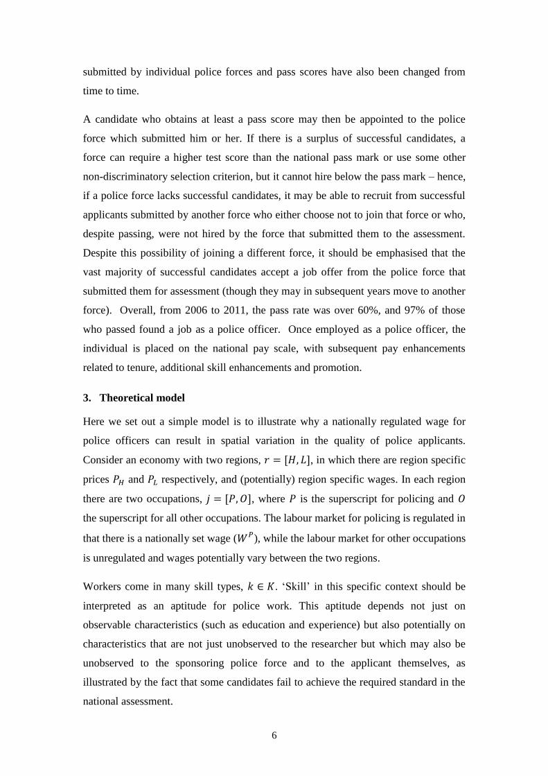
Table 1: Matrix of competency areas assessed by exercise, 2008

Exercises

Interactive Written Psychometric Tests

1 2 3 4 1 2 Interview

Verbal

logical

reasoning

Numerical

reasoning

Co

mp

eten

cy a

rea

s

Community &

Customer Focus

Effective

Communication

Oral

Communication

Written

Communication

Personal

Responsibility

Problem

Solving

Resilience

Respect for Race

& Diversity

Teamworking

23

2: Distribution of candidate test scores, 2008

Notes: In 2008 the required marks to pass the SEARCH assessment were 44% for written communication, 50% for

oral communication, 50% for Respect for Race and Diversity and 50% overall.

Figure 3. Distribution of police force area fixed effects on outside wages

0%

5%

10%

15%

20%

25%

0 10 20 30 40 50 60 70 80 90 100

Pro

po

rtio

n o

f ca

nd

idat

es

Written score (percent)

0%

10%

20%

30%

40%

50%

60%

70%

0 10 20 30 40 50 60 70 80 90 100

Oral score (percent)

0%

5%

10%

15%

20%

25%

0 10 20 30 40 50 60 70 80 90 100

Pro

po

rtio

n o

f ca

nd

idat

es

RfRD score (percent)

-1%

1%

3%

5%

7%

9%

0 10 20 30 40 50 60 70 80 90 100

Overall score (percent)

-0.20

-0.15

-0.10

-0.05

0.00

0.05

0.10

0.15

0.20

0.25

0.30

Dyf

ed P

ow

ys

Dev

on

an

d C

orn

wal

l C

um

bri

a H

um

ber

sid

e D

urh

am

Cle

vela

nd

N

orf

olk

W

est

Mer

cia

Sou

th Y

ork

shir

e

No

rth

Wal

es

Gw

ent

No

rth

Yo

rksh

ire

Do

rset

So

uth

Wal

es

Lan

cash

ire

Der

bys

hir

e N

ort

hu

mb

ria

Lin

coln

shir

e St

affo

rdsh

ire

Mer

seys

ide

No

ttin

gham

shir

e G

lou

cest

ersh

ire

Suff

olk

So

mer

set

and

Avo

n

Wes

t M

idla

nd

s W

est

York

shir

e Le

ices

ters

hir

e G

reat

er M

anch

este

r Su

ssex

C

hes

hir

e H

amp

shir

e W

arw

icks

hir

e W

iltsh

ire

Ken

t N

ort

ham

pto

nsh

ire

B

edfo

rdsh

ire

Esse

x C

amb

rid

gesh

ire

Tham

es V

alle

y Su

rrey

H

ertf

ord

shir

e Lo

nd

on

Met

24

Table 2: Characteristics associated with candidates’ test scores

Written

score

Oral

score

RFD

score

Overall score Pr(pass)

2008 -3.858 -0.248 0.433 -0.635 -0.036

(8.64)** (1.72) (2.36)* (4.20)** (3.95)**

2009 -11.381 1.082 1.332 -2.822 -0.124

(25.32)** (7.48)** (7.21)** (18.52)** (13.66)**

2010 -1.931 1.576 -0.171 0.566 0.010

(3.48)** (8.82)** (0.75) (3.01)** (0.88)

Age 1.224 0.558 1.045 0.930 0.038

(10.47)** (14.84)** (21.79)** (23.49)** (15.98)**

Age squared -0.019 -0.009 -0.016 -0.014 -0.001

(9.82)** (14.66)** (20.50)** (22.42)** (15.31)**

Male -2.434 -1.014 -2.255 -1.820 -0.062

(10.77)** (13.93)** (24.30)** (23.75)** (13.58)**

GCSEs 1.840 1.082 0.176 0.371 0.012

(3.48)** (6.36)** (0.81) (2.07)* (1.11)

A levels 5.933 1.736 1.813 2.397 0.098

(11.24)** (10.22)** (8.36)** (13.40)** (9.19)**

Graduate 9.767 2.381 3.303 4.491 0.168

(18.22)** (13.80)** (15.00)** (24.71)** (15.55)**

Experience: PCSO 2.685 2.006 3.902 4.003 0.132

(9.12)** (21.17)** (32.29)** (40.11)** (22.29)**

Experience: SC 3.120 1.473 2.682 2.860 0.092

(8.30)** (12.17)** (17.38)** (22.45)** (12.18)**

Mixed white -3.395 -0.161 0.139 -0.512 -0.031

(5.17)** (0.76) (0.51) (2.30)* (2.35)*

Asian -15.309 -2.801 -2.190 -3.793 -0.209

(32.84)** (18.67)** (11.44)** (24.00)** (22.24)**

African -19.627 -4.656 -1.827 -5.436 -0.288

(27.93)** (20.59)** (6.33)** (22.82)** (20.33)**

Chinese -10.194 -3.974 -1.614 -2.433 -0.103

(5.63)** (6.82)** (2.17)* (3.97)** (2.83)**

Other -19.962 -5.271 -2.486 -5.903 -0.269

(13.17)** (10.80)** (3.99)** (11.49)** (8.82)**

Missing ethnicity -3.939 -0.702 -1.012 -1.126 -0.053

(9.12)** (5.05)** (5.71)** (7.69)** (6.14)**

Constant 47.661 86.282 49.329 42.231 0.176

(25.94)** (145.90)** (65.39)** (67.80)** (4.75)**

R-squared 0.11 0.06 0.08 0.16 0.08

Notes: Sample size is 41,485 individuals. Figures are marginal effects from linear regression (first four columns)

and linear probability model (final column). Baseline candidate is female, with no qualifications, no previous

experience in the police, and of white ethnicity. Standard errors are in parentheses. ***, ** and * indicate

statistical significance at the 1%, 5% and 10% level respectively.

25

Table 3. Distribution of average candidate performance, candidate composition, local

area characteristics, and the disamenity of policing across forces and time

Mean Standard

deviation

25th

percentile Median

75th

percentile

Candidate performance Pass rate 75.6 14.857 70.8 77.5 83.7 Mean score:

Written communication 64.8 8.478 60.3 66.1 69.5 Oral communication 95.8 2.177 94.9 96.0 97.2 Respect for Race and Diversity 66.7 4.234 64.9 67.0 68.5 Overall 57.3 2.876 55.4 57.3 59.0

Candidate characteristics

Mean age 26.6 2.057 25.9 26.7 27.3 % male 68.0 11.109 62.6 66.7 71.1 % with only A-levels 38.8 14.790 34.5 39.2 43.3 % with degree 27.8 16.402 21.2 28.1 32.1 % with experience 27.0 18.841 17.1 25.0 33.0 % white 86.0 15.533 82.9 90.8 94.6

Local area characteristics

% of population with degree 33.6 9.489 28.3 31.1 36.9 % of population with only A-levels 20.1 3.421 19.3 20.6 21.9 % of population with only GCSEs 22.8 4.201 21.6 23.6 25.4 Unemployment rate (%) 4.3 2.072 3.0 4.0 4.9 Median house price (£,000s) 158.1 52.607 119.3 145.0 175.0

Disamenity of policing

Crime per 1000 population 7.3 1.759 6.2 7.2 8.3 % crime: theft 17.5 4.441 15.7 16.9 18.4 % crime: criminal damage 22.0 4.384 20.5 22.4 24.6 % crime: domestic burglary 5.2 1.677 4.2 5.2 6.3 % crime: drugs offences 4.4 2.260 3.2 3.9 4.5 % crime: non-domestic burglary 6.7 1.055 6.1 6.6 7.4 % crime: public order offences 4.4 1.185 3.5 4.2 5.1 % crime: shoplifting 6.9 1.501 5.9 6.9 7.8 % crime: vehicle offences 12.2 2.811 10.6 12.2 14.2 % crime: violence without injury 9.9 1.752 8.8 9.7 11.0 % crime: violence with injury 1.1 0.856 0.6 0.8 1.3

Notes: Distributions are calculated over 133 force-time observations (42 forces, observed

between once and four times).

26

Table 4. Association of applicant quality with outside wage

Written

communication

(%)

Oral

communication

(%)

Respect for

Race and

Diversity

(%)

Overall

(%)

Pr.(Pass)

-11.104 11.752 -9.087 -9.539 -0.116

(2.824)*** (0.924)*** (1.350)*** (1.029)*** (0.060)*

2008 -2.725 -0.069 0.815 -0.246 -0.018

(0.446)*** (0.159) (0.217)*** (0.160) (0.009)*

2009 -10.612 1.185 1.983 -2.210 -0.100

(0.517)*** (0.178)*** (0.242)*** (0.191)*** (0.011)***

2010 -2.495 2.195 0.327 1.124 0.038

(0.620)*** (0.201)*** (0.274) (0.228)*** (0.013)***

London -0.663 -0.899 -0.116 -0.877 -0.018

(0.761) (0.249)*** (0.338) (0.278)*** (0.015)

% with degree -0.312 -0.050 0.076 0.005 -0.003

(0.063)*** (0.018)** (0.028)*** (0.022) (0.001)**

% with A-levels -0.228 -0.024 0.123 0.023 -0.001

(0.120)* (0.038) (0.057)** (0.044) (0.003)

% with no qualifications -0.596 -0.038 0.011 -0.020 -0.004

(0.076)*** (0.022) (0.034) (0.027) (0.002)**

Unemployment rate 0.297 -0.052 -0.125 0.017 -0.001

(0.094)*** (0.024) (0.038)*** (0.031) (0.002)

Av. house price (£,000s) 0.028 -0.012 0.019 0.028 0.001

(0.008)*** (0.002)*** (0.004)*** (0.003)*** (0.000)***

R-Squared 0.05 0.02 0.01 0.04 0.02

F(10,41474) 228.17 71.62 40.11 153.65 70.90

Notes: Sample size is 41,485. Bootstrapped standard errors, 999 replications.

27

Table 5. Association of applicant quality with outside wage; controlling for disutility of

policing

Written

communication

(%)

Oral

communicatio

n

(%)

Respect for

Race and

Diversity

(%)

Overall

(%)

Pr.(Pass)

-21.294 9.388 -18.659 -13.196 -0.310

(3.838)*** (1.286)*** (1.844)*** (1.409)*** (0.080)***

2008 -3.355 -0.343 0.320 -1.136 -0.060

(0.565)*** (0.186)* (0.256) (0.204)*** (0.011)***

2009 -10.988 0.115 0.430 -4.216 -0.187

(0.823)*** (0.285) (0.381) (0.306)*** (0.017)***

2010 -2.288 0.787 -1.133 -1.166 -0.055

(0.986)** (0.331)** (0.445)*** (0.360)*** (0.020)***

London 2.302 -0.997 5.110 3.541 0.171

(1.369) (0.458)** (0.625)*** (0.485)*** (0.029)***

% with degree -0.317 -0.046 0.049 0.070 -0.001

(0.078)*** (0.023)* (0.036) (0.028)** (0.002)

% with A-levels -0.419 0.071 -0.028 0.096 0.001

(0.147)*** (0.047) (0.071) (0.057)* (0.003)

% with no qualifications -0.403 -0.095 0.012 0.082 -0.000

(0.106)*** (0.030)*** (0.046) (0.038)** (0.002)

Unemployment rate 0.422 0.084 0.395 0.330 0.012

(0.159)*** (0.048)* (0.068)*** (0.053)*** (0.003)***

Av. house price (£,000s) 0.051 -0.014 0.025 0.032 0.001

(0.012)*** (0.004)*** (0.005)*** (0.004)*** (0.000)**

Proportion of crime:

Theft 0.496 -0.384 -0.177 -0.156 -0.005

(0.167)*** (0.057)*** (0.079)** (0.060)** (0.003)

Criminal damage 0.429 -0.399 -0.234 -0.149 -0.006

(0.156)** (0.057)*** (0.072)*** (0.058)** (0.003)*

Domestic burglary 1.343 -0.078 0.488 0.638 0.026

(0.245)*** (0.074) (0.109)*** (0.089)*** (0.005)***

Drugs offences 0.090 -0.058 -0.410 -0.105 -0.005

(0.162) (0.051) (0.072)*** (0.060)* (0.003)

Non-dom. burglary -0.536 0.248 -0.361 0.044 -0.003

(0.287)* (0.090)** (0.127)*** (0.106) (0.006)

Public order offences -0.116 -0.441 -0.023 -0.170 -0.009

(0.215) (0.072)*** (0.100) (0.078)** (0.004)**

Shoplifting 0.166 -0.400 -0.177 0.017 -0.004

(0.231) (0.077)*** (0.106)* (0.086) (0.005)

Vehicle offences 0.384 -0.304 0.172 0.056 0.004

(0.151)** (0.051)*** (0.070)*** (0.058) (0.003)

Violence without injury 0.067 -0.365 -0.406 -0.088 -0.008

(0.204) (0.070)*** (0.094)*** (0.075) (0.004)*

Violence with injury -1.846 -0.410 -2.069 -1.822 -0.072

(0.356)*** (0.120)*** (0.165)*** (0.128)*** (0.008)***

Crime per 1000 head -0.554 0.103 -0.435 -0.394 -0.023

(0.214)** (0.068) (0.096)*** (0.081)*** (0.004)***

R-squared 0.06 0.02 0.02 0.04 0.02

F(21,41463) 115.63 45.83 37.05 90.67 43.68

Notes: Sample size is 41,485. Standard errors are bootstrapped, 999 replications.

28

Table 6. Sensitivity analysis

Written

communication

(%)

Oral

communication

(%)

Respect for

Race and

Diversity

(%)

Overall

(%)

Pr.(Pass)

Baseline (LFS, all)

-21.294 9.388 -18.659 -13.196 -0.310

(3.838)*** (1.286)*** (1.844)*** (1.409)*** (0.080)***

Violence without injury 0.067 -0.365 -0.406 -0.088 -0.008

(0.204) (0.070)*** (0.094)*** (0.075) (0.004)*

Violence with injury -1.846 -0.410 -2.069 -1.822 -0.072

(0.356)*** (0.120)*** (0.165)*** (0.128)*** (0.008)***

Crime per 1000 head -0.554 0.103 -0.435 -0.394 -0.023

(0.214)** (0.068) (0.096)*** (0.081)*** (0.004)***

R-squared 0.06 0.02 0.02 0.04 0.02

ASHE, excl. police wage

-14.404 5.777 -15.762 -8.595 -0.189

(4.938)*** (1.576)*** (2.036)*** (1.735)*** (0.100)*

Violence without injury 0.324 -0.477 -0.176 0.070 -0.004

(0.209) (0.067)*** (0.086)** (0.073) (0.004)

Violence with injury -1.602 -0.514 -1.838 -1.673 -0.068

(0.377)*** (0.120)*** (0.156)*** (0.133)*** (0.008)***

Crime per 1000 head -0.160 -0.063 -0.051 -0.154 -0.018

(0.223) (0.071) (0.092) (0.079)* (0.005)***

R-squared 0.05 0.02 0.02 0.04 0.02

ASHE, incl. police wage

16.182 -1.918 11.159 6.525 0.273

(2.680)*** (0.856)** (1.105)*** (0.941)*** (0.054)***

Violence without injury 0.442 -0.485 -0.103 0.114 -0.002

(0.210)** (0.067)*** (0.087) (0.074) (0.004)

Violence with injury -1.915 -0.454 -2.087 -1.815 -0.073

(0.378)*** (0.121)*** (0.156)*** (0.133)*** (0.008)***

Crime per 1000 head 0.046 -0.037 0.020 -0.105 -0.014

(0.224) (0.072) (0.092) (0.079) (0.005)***

R-squared 0.06 0.02 0.02 0.04 0.02

Notes: Sample size is 41,485. All regressions are the same specification as presented in Table

5. For brevity only a limited number of coefficients are reported here; full results are available

on request. Standard errors in the baseline regression are bootstrapped, 999 replications.

29

Table 7. Association of applicant quality with outside wage; controlling for applicant

characteristics

Written

communication

(%)

Oral

communication

(%)

Respect for

Race and

Diversity

(%)

Overall

(%)

Pr.(Pass)

Without controls for

applicant characteristics:

-21.294 9.388 -18.659 -13.196 -0.310

(3.838)*** (1.286)*** (1.844)*** (1.409)*** (0.080)***

Violence without injury 0.067 -0.365 -0.406 -0.088 -0.008

(0.204) (0.070)*** (0.094)*** (0.075) (0.004)*

Violence with injury -1.846 -0.410 -2.069 -1.822 -0.072

(0.356)*** (0.120)*** (0.165)*** (0.128)*** (0.008)***

Crime per 1000 head -0.554 0.103 -0.435 -0.394 -0.023

(0.214)** (0.068) (0.096)*** (0.081)*** (0.004)***

R-squared 0.06 0.02 0.02 0.04 0.02

With controls for

applicant characteristics

-14.371 11.545 -15.364 -9.581 -0.162

(3.697)*** (1.273)*** (1.777)*** (1.360)*** (0.079)**

Violence without injury 0.131 -0.365 -0.400 -0.070 -0.007

(0.199) (0.068)*** (0.091)*** (0.070) (0.004)*

Violence with injury -0.761 -0.089 -1.562 -1.212 -0.048

(0.345)** (0.117) (0.159)*** (0.119)*** (0.007)***

Crime per 1000 head -0.568 0.099 -0.439 -0.401 -0.024

(0.207)*** (0.067) (0.092)*** (0.077)*** (0.004)***

R-squared 0.12 0.08 0.09 0.17 0.08

Notes: Sample size is 41.485. Standard errors are bootstrapped, 999 replications.

30

Table 8. Association of applicant characteristics with outside wage and disamenity of

policing

Age Pr(Female) Pr(Experience) Pr(A-levels

or above)

Pr(White)

-7.030 -0.302 -0.145 -0.135 -0.232

(1.221)*** (0.093)*** (0.086)* (0.087) (0.058)***

2008 0.166 0.004 0.048 -0.016 0.017

(0.168) (0.012) (0.011)*** (0.012) (0.010)*

2009 0.789 -0.004 0.067 -0.103 0.012

(0.261)*** (0.019) (0.017)*** (0.019)*** (0.014)

2010 0.952 0.022 0.122 -0.099 -0.014

(0.314)*** (0.023) (0.021)*** (0.022)*** (0.017)

London 1.420 0.002 0.142 0.231 0.026

(0.418)*** (0.031) (0.028)*** (0.031)*** (0.022)

% with degree 0.060 0.001 -0.001 0.005 0.001

(0.022)** (0.001) (0.002) (0.002)*** (0.001)

% with A-levels 0.030 -0.003 -0.009 0.012 0.002

(0.044) (0.003) (0.003)*** (0.003)*** (0.002)

% with no qualifications 0.080 -0.001 0.003 0.001 0.004

(0.030)** (0.002) (0.002) (0.002) (0.002)**

Unemployment rate -0.032 0.002 0.007 0.010 0.005

(0.047) (0.003) (0.003)** (0.003)*** (0.002)*

Av. house price (£,000s) 0.013 0.001 0.001 -0.001 0.000

(0.004)*** (0.000)** (0.000)** (0.000)*** (0.001)

Proportion of crime:

Theft 0.191 -0.002 0.007 -0.016 -0.005

(0.052)*** (0.004) (0.004)** (0.004)*** (0.003)*

Criminal damage 0.116 0.006 0.005 -0.026 -0.008

(0.051)** (0.004) (0.003) (0.004)*** (0.003)***

Domestic burglary 0.086 0.008 0.011 -0.010 0.002

(0.071) (0.006) (0.005)** (0.006)* (0.004)

Drugs offences -0.004 -0.002 -0.009 -0.000 0.000

(0.048) (0.004) (0.003)*** (0.003) (0.002)

Non-dom. burglary 0.209 -0.013 0.006 0.023 0.013

(0.086)** (0.007)** (0.006) (0.006)*** (0.005)**

Public order offences 0.268 -0.007 -0.000 -0.004 -0.003

(0.067)*** (0.005) (0.005) (0.005) (0.003)

Shoplifting 0.128 -0.003 -0.008 -0.003 0.006

(0.069)* (0.005) (0.005) (0.005) (0.003)

Vehicle offences 0.087 0.002 0.000 -0.002 -0.003

(0.044)* (0.003) (0.003) (0.003) (0.002)

Violence without injury 0.145 0.006 0.002 -0.016 -0.011

(0.061)** (0.005) (0.004) (0.005)*** (0.003)***

Violence with injury -0.017 -0.009 -0.054 -0.084 -0.067

(0.108) (0.008) (0.007)*** (0.008)*** (0.006)***

Crime per 1000 head 0.024 -0.002 -0.002 -0.003 0.002

(0.061) (0.005) (0.004) (0.005) (0.003)

R-squared 0.01 0.01 0.01 0.01 0.05

F(21,41463) 16.07 6.58 26.70 19.11 103.67

Notes: Sample size is 41,485. Standard errors are bootstrapped, 999 replications.