Embed Size (px)
Citation preview

Principles of MRI Principles of MRI Physics and EngineeringPhysics and Engineering
Allen W. Song Allen W. Song
Brain Imaging and Analysis CenterBrain Imaging and Analysis Center
Duke UniversityDuke University
What if the RF field is not synchronized?
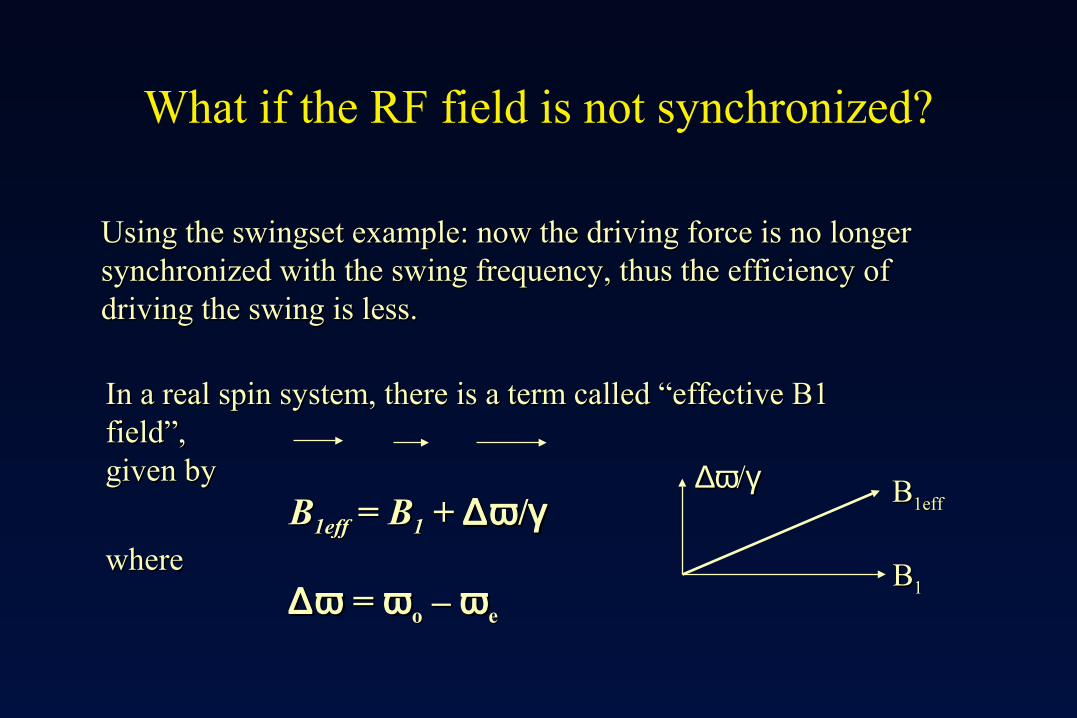
Using the swingset example: now the driving force is no longer Using the swingset example: now the driving force is no longer synchronized with the swing frequency, thus the efficiency of synchronized with the swing frequency, thus the efficiency of driving the swing is less.driving the swing is less.
In a real spin system, there is a term called “effective B1 In a real spin system, there is a term called “effective B1 field”,field”,given by given by
BB1eff1eff = = BB11 + + ∆ω∆ω //γγwhere where
∆ω∆ω = = ωω oo – – ωω e e
BB11
BB1eff1eff∆ω∆ω//γγ

Part II.1Part II.1
Image FormationImage Formation
What is image formation?
To define the spatial location of the protonTo define the spatial location of the protonpools that contribute to the MR signal afterpools that contribute to the MR signal afterspin excitation.spin excitation.
A 3-D gradient field (dB/dx, dB/dy, dB/dz) would A 3-D gradient field (dB/dx, dB/dy, dB/dz) would allow a unique correspondence between the spatial allow a unique correspondence between the spatial location and the magnetic field. Using this information,location and the magnetic field. Using this information,we will be able to generate maps that contain spatial we will be able to generate maps that contain spatial information – images.information – images.
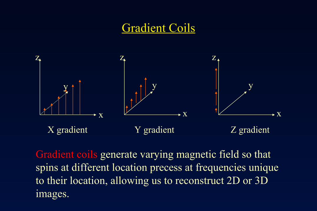
Gradient Coils
Gradient coils generate varying magnetic field so that spins at different location precess at frequencies uniqueto their location, allowing us to reconstruct 2D or 3Dimages.
X gradient Y gradient Z gradient
x
y
z
x
z z
x
y y
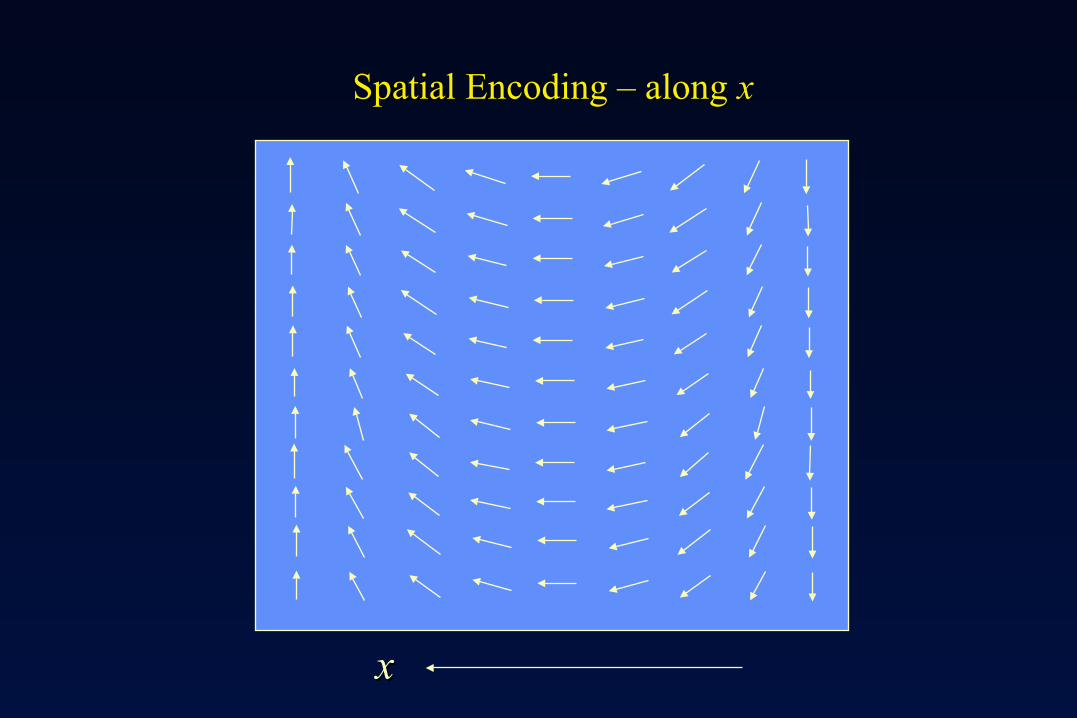
Spatial Encoding – along Spatial Encoding – along xx
xx
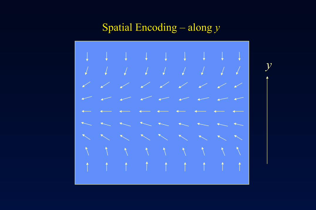
Spatial Encoding – along Spatial Encoding – along yy
yy
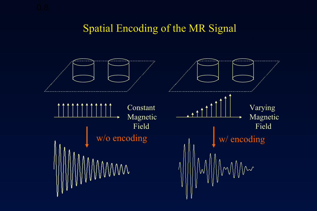
Spatial Encoding of the MR Signal
0.8
w/o encoding w/ encoding
ConstantMagnetic Field
VaryingMagnetic Field
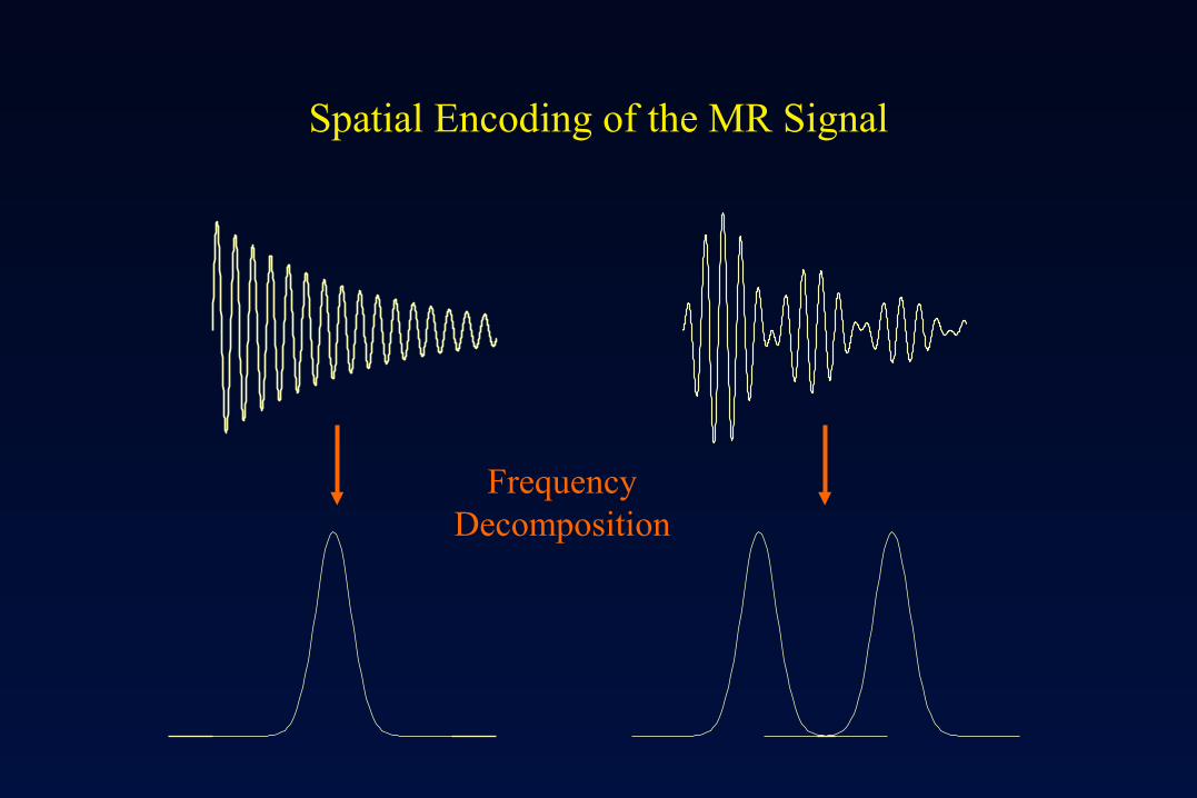
Spatial Encoding of the MR Signal
FrequencyDecomposition
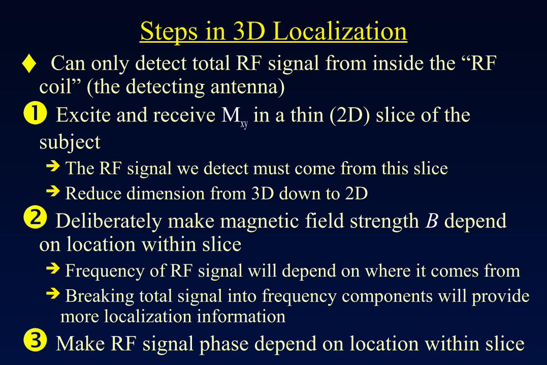
Steps in 3D Localization♦ Can only detect total RF signal from inside the “RF
coil” (the detecting antenna)
Excite and receive Mxy in a thin (2D) slice of the subject The RF signal we detect must come from this slice Reduce dimension from 3D down to 2D
Deliberately make magnetic field strength B depend on location within slice Frequency of RF signal will depend on where it comes from Breaking total signal into frequency components will provide
more localization information
Make RF signal phase depend on location within slice
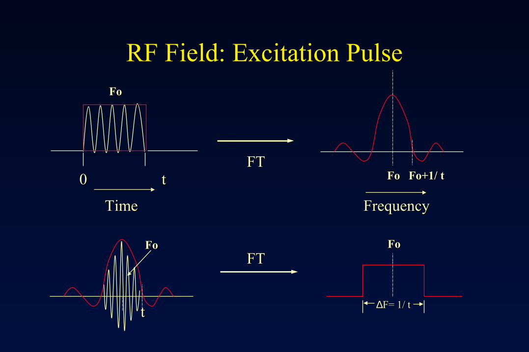
RF Field: Excitation Pulse
00 tt
FoFo
FoFo Fo+1/ tFo+1/ t
TimeTime FrequencyFrequency
tt
FoFo FoFo
∆∆F= 1/ tF= 1/ t
FTFT
FTFT
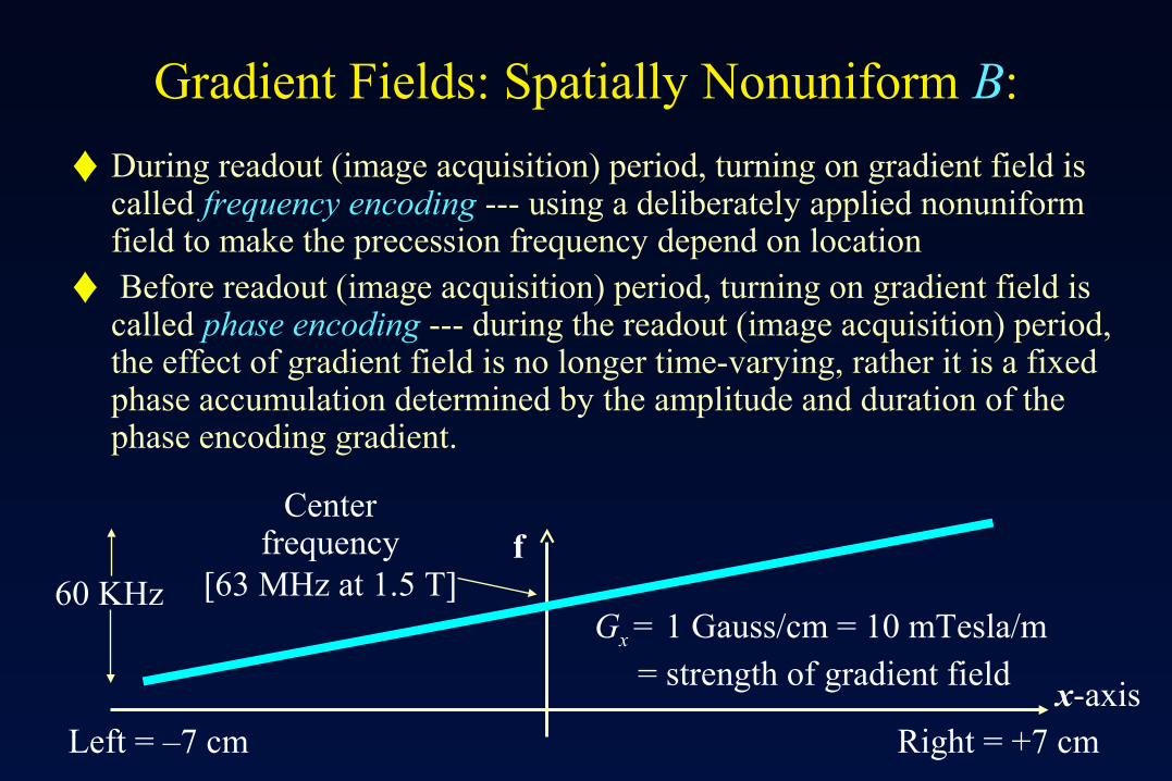
Gradient Fields: Spatially Nonuniform B:
♦During readout (image acquisition) period, turning on gradient field is called frequency encoding --- using a deliberately applied nonuniform field to make the precession frequency depend on location
♦ Before readout (image acquisition) period, turning on gradient field is called phase encoding --- during the readout (image acquisition) period, the effect of gradient field is no longer time-varying, rather it is a fixed phase accumulation determined by the amplitude and duration of the phase encoding gradient.
x-axis
f60 KHz
Left = –7 cm Right = +7 cm
Gx = 1 Gauss/cm = 10 mTesla/m = strength of gradient field
Centerfrequency
[63 MHz at 1.5 T]
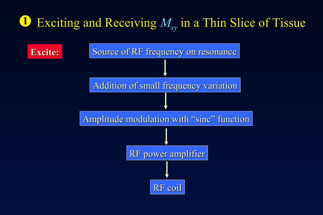
Exciting and Receiving Mxy in a Thin Slice of Tissue
Source of RF frequency on resonanceSource of RF frequency on resonance
Addition of small frequency variationAddition of small frequency variation
Amplitude modulation with “sinc” functionAmplitude modulation with “sinc” function
RF power amplifierRF power amplifier
RF coilRF coil
Excite:Excite:
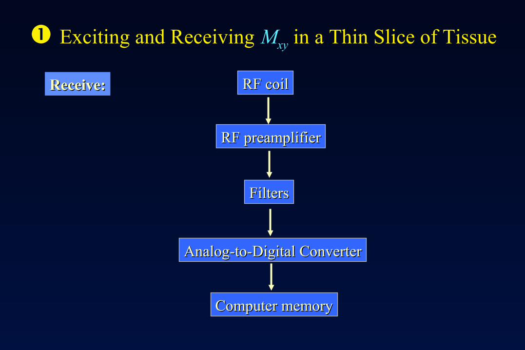
Exciting and Receiving Mxy in a Thin Slice of Tissue
RF coilRF coil
RF preamplifierRF preamplifier
FiltersFilters
Analog-to-Digital ConverterAnalog-to-Digital Converter
Computer memoryComputer memory
Receive:Receive:
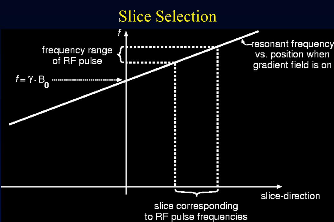
Slice Selection
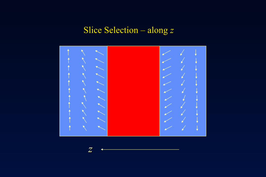
Slice Selection – along Slice Selection – along zz
zz
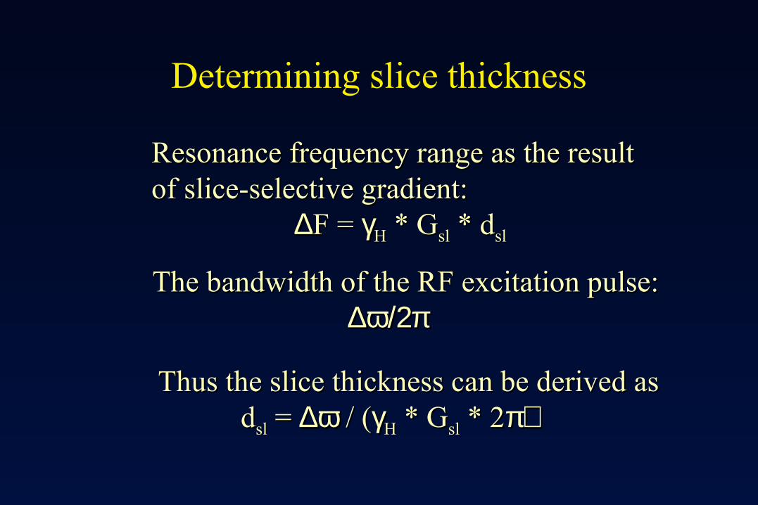
Determining slice thickness
Resonance frequency range as the resultResonance frequency range as the resultof slice-selective gradient:of slice-selective gradient: ∆ ∆F = F = γγHH * G * Gslsl * d * dslsl
The bandwidth of the RF excitation pulse:The bandwidth of the RF excitation pulse: ∆ω/2π∆ω/2π
Thus the slice thickness can be derived asThus the slice thickness can be derived as ddslsl = = ∆ω∆ω / ( / (γγHH * G * Gslsl * 2 * 2π)π)
Changing slice thickness
There are two ways to do this:There are two ways to do this:
(a)(a) Change the slope of the slice selection gradientChange the slope of the slice selection gradient
(b)(b) Change the bandwidth of the RF excitation pulseChange the bandwidth of the RF excitation pulse
Both are used in practice, with (a) being more popularBoth are used in practice, with (a) being more popular
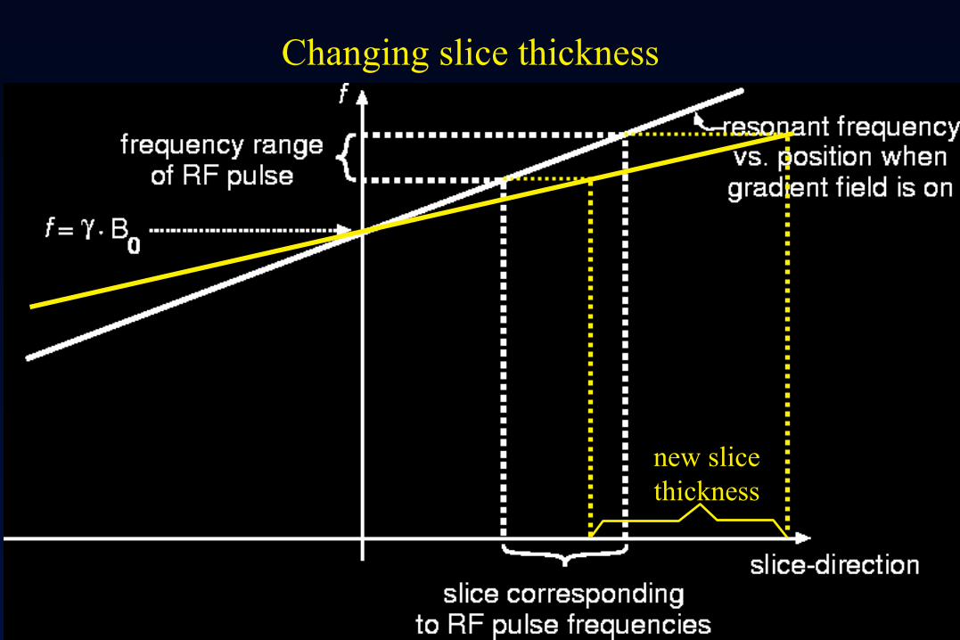
Changing slice thickness
new slicenew slicethicknessthickness
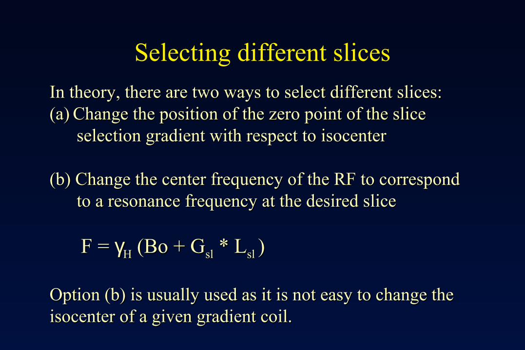
Selecting different slices
In theory, there are two ways to select different slices:In theory, there are two ways to select different slices:(a)(a) Change the position of the zero point of the sliceChange the position of the zero point of the slice selection gradient with respect to isocenterselection gradient with respect to isocenter
(b) Change the center frequency of the RF to correspond(b) Change the center frequency of the RF to correspond to a resonance frequency at the desired sliceto a resonance frequency at the desired slice
F = F = γγHH (Bo + G (Bo + Gslsl * L * Lsl sl ))
Option (b) is usually used as it is not easy to change theOption (b) is usually used as it is not easy to change theisocenter of a given gradient coil.isocenter of a given gradient coil.

Selecting different slices
new slicenew slicelocationlocation
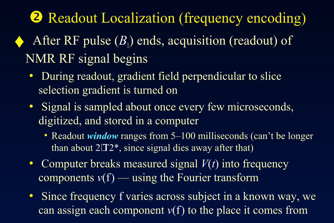
Readout Localization (frequency encoding)
♦ After RF pulse (B1) ends, acquisition (readout) of NMR RF signal begins• During readout, gradient field perpendicular to slice
selection gradient is turned on
• Signal is sampled about once every few microseconds, digitized, and stored in a computer
• Readout window ranges from 5–100 milliseconds (can’t be longer than about 2⋅T2*, since signal dies away after that)
• Computer breaks measured signal V(t) into frequency components v(f ) — using the Fourier transform
• Since frequency f varies across subject in a known way, we can assign each component v(f ) to the place it comes from
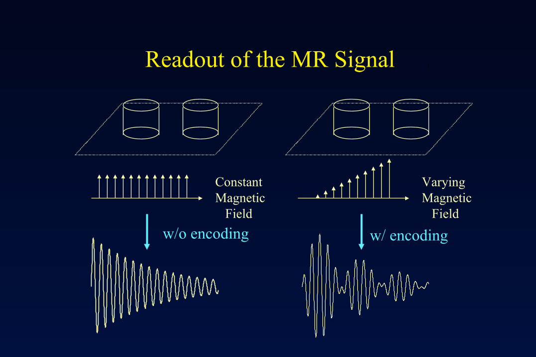
Readout of the MR Signal
w/o encoding w/ encoding
ConstantMagnetic Field
VaryingMagnetic Field
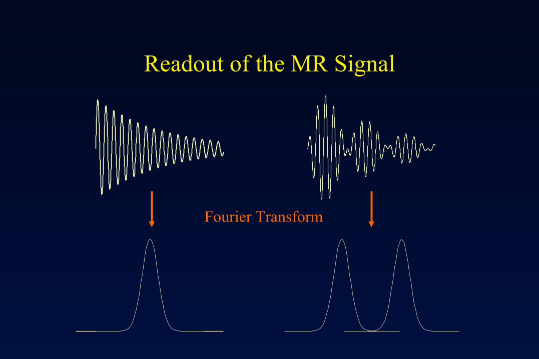
Readout of the MR Signal
Fourier Transform
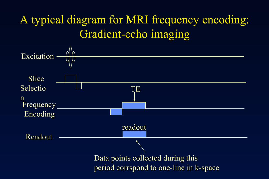
A typical diagram for MRI frequency encoding:Gradient-echo imaging
readoutreadout
ExcitationExcitation
SliceSliceSelectioSelectionnFrequencyFrequency EncodingEncoding
ReadoutReadout
TETE
Data points collected during thisData points collected during thisperiod corrspond to one-line in k-spaceperiod corrspond to one-line in k-space
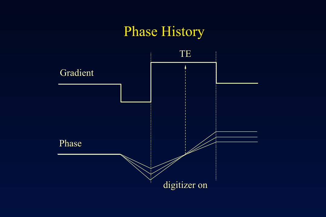
PhasePhase
Phase HistoryPhase History
digitizer ondigitizer on
GradientGradient
TETE
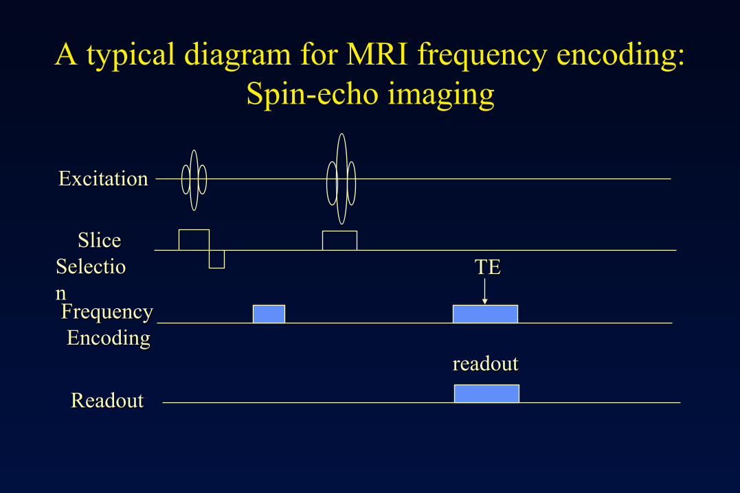
A typical diagram for MRI frequency encoding:Spin-echo imaging
readoutreadout
ExcitationExcitation
SliceSliceSelectioSelectionnFrequencyFrequency EncodingEncoding
ReadoutReadout
TETE
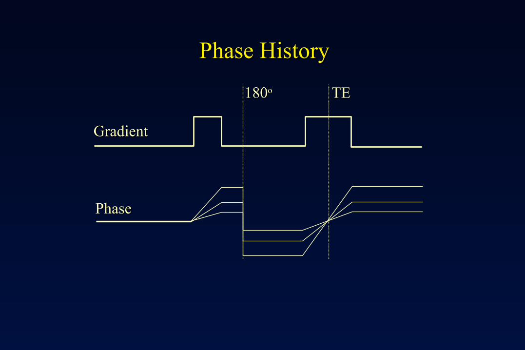
180180oo TETE
PhasePhase
Phase HistoryPhase History
GradientGradient
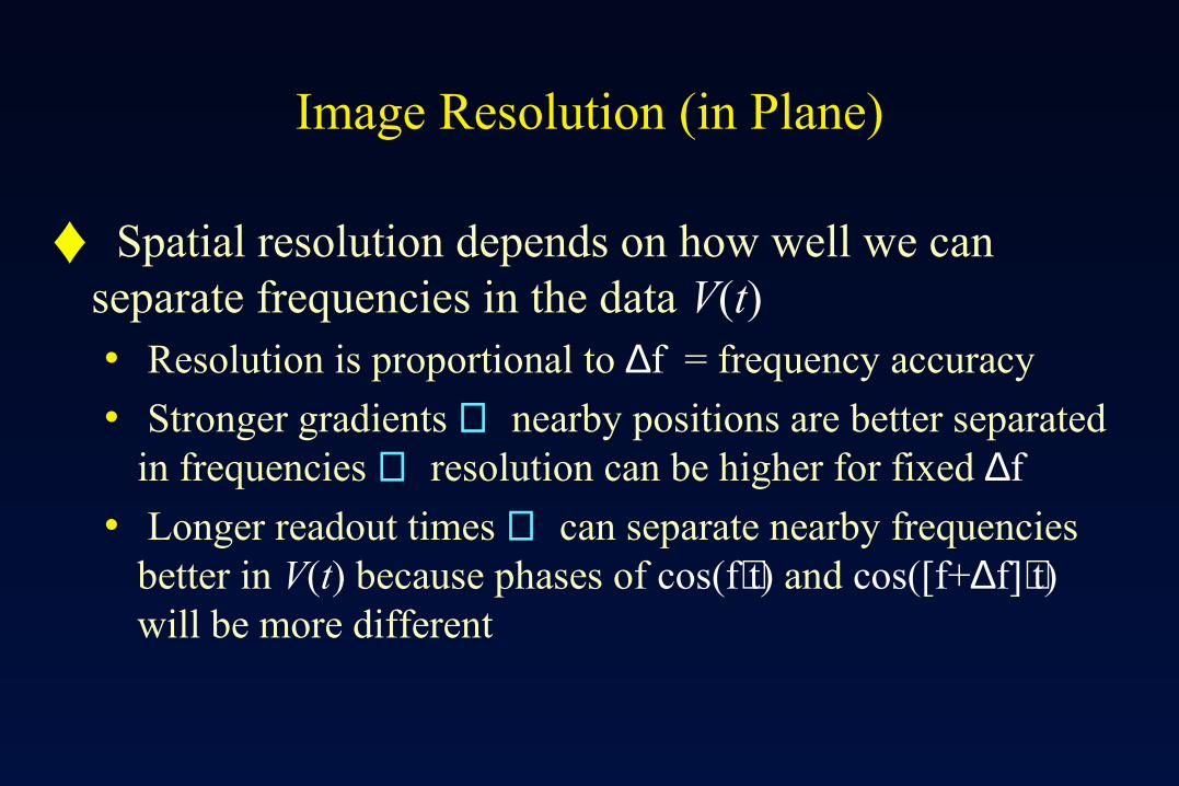
Image Resolution (in Plane)
♦ Spatial resolution depends on how well we can separate frequencies in the data V(t)• Resolution is proportional to ∆f = frequency accuracy
• Stronger gradients ⇒ nearby positions are better separated in frequencies ⇒ resolution can be higher for fixed ∆f
• Longer readout times ⇒ can separate nearby frequencies better in V(t) because phases of cos(f⋅t) and cos([f+∆f]⋅t) will be more different
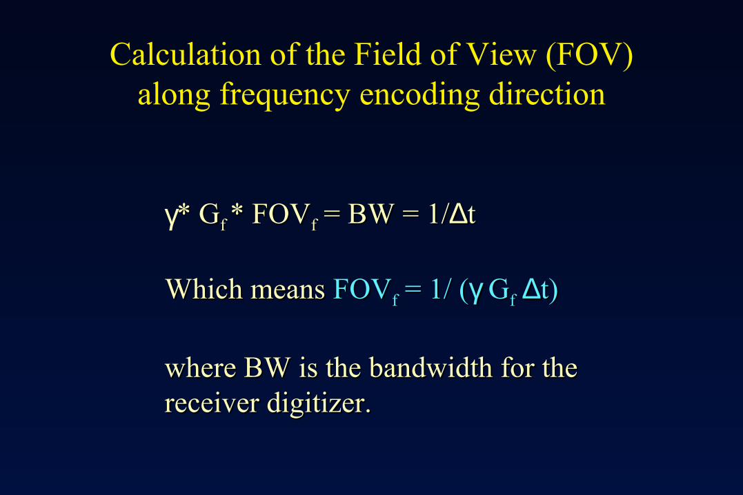
Calculation of the Field of View (FOV)along frequency encoding direction
γ* G* Gf f * FOV* FOVff = BW = 1/ = BW = 1/∆∆tt
Which means Which means FOVFOVff = 1/ ( = 1/ (γγ G Gff ∆∆t)t)
where BW is the bandwidth for thewhere BW is the bandwidth for thereceiver digitizer.receiver digitizer.
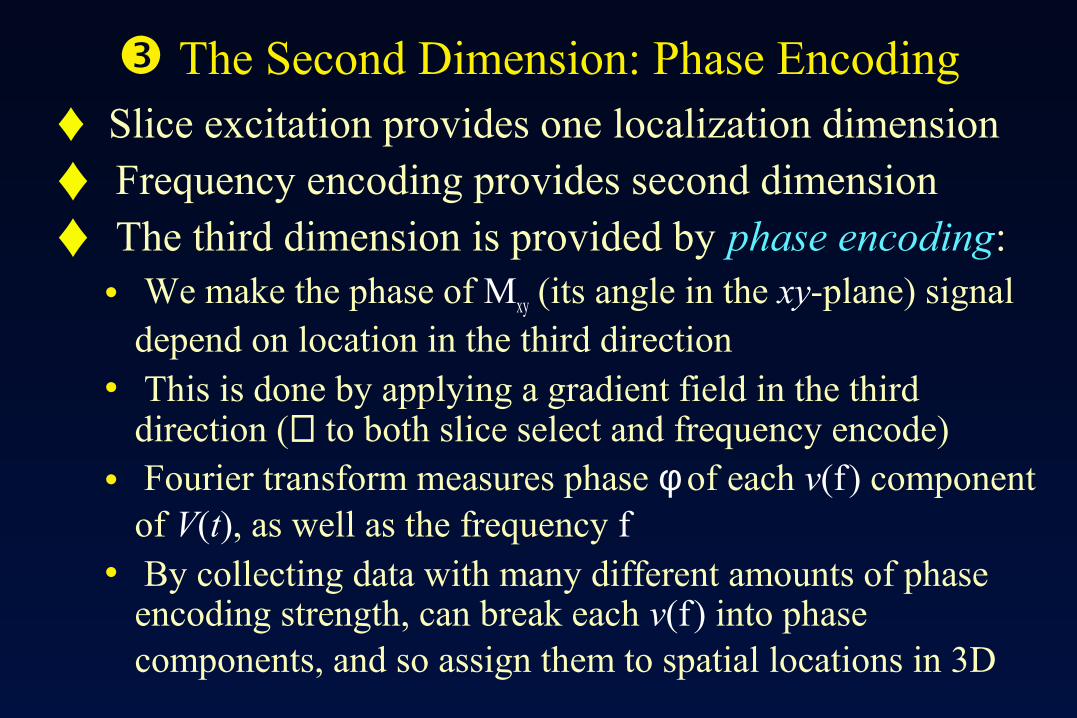
The Second Dimension: Phase Encoding
♦ Slice excitation provides one localization dimension
♦ Frequency encoding provides second dimension
♦ The third dimension is provided by phase encoding:• We make the phase of Mxy (its angle in the xy-plane) signal
depend on location in the third direction• This is done by applying a gradient field in the third
direction (⊥ to both slice select and frequency encode)• Fourier transform measures phase φ of each v(f ) component
of V(t), as well as the frequency f• By collecting data with many different amounts of phase
encoding strength, can break each v(f ) into phase components, and so assign them to spatial locations in 3D
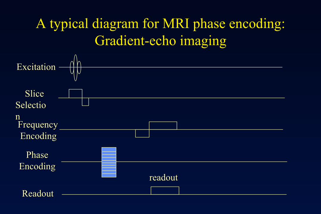
A typical diagram for MRI phase encoding:Gradient-echo imaging
readoutreadout
ExcitationExcitation
SliceSliceSelectioSelectionnFrequencyFrequency EncodingEncoding
PhasePhase EncodingEncoding
ReadoutReadout
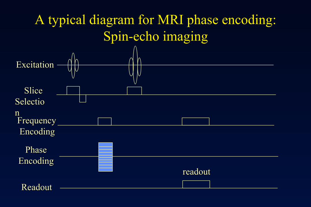
A typical diagram for MRI phase encoding:Spin-echo imaging
readoutreadout
ExcitationExcitation
SliceSliceSelectioSelectionnFrequencyFrequency EncodingEncoding
PhasePhase EncodingEncoding
ReadoutReadout
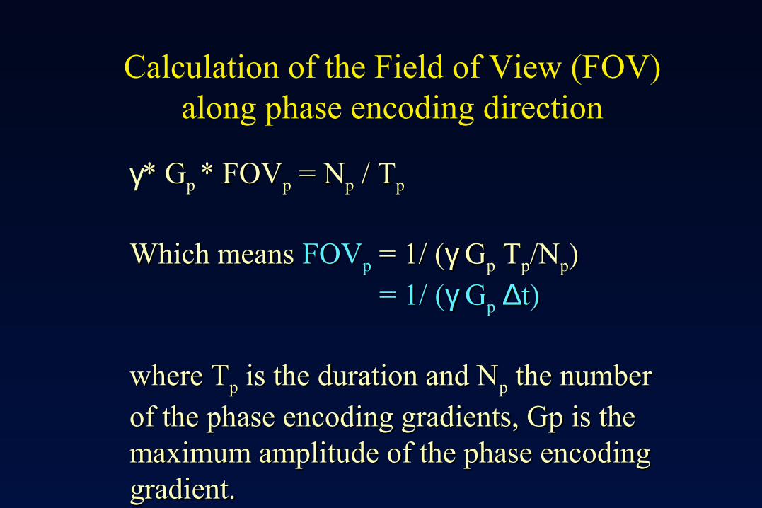
Calculation of the Field of View (FOV)along phase encoding direction
γ* G* Gp p * FOV* FOVpp = N = Npp / T / Tpp
Which means Which means FOVFOVpp = 1/ ( = 1/ (γγ G Gpp T Tpp/N/Npp))
= 1/ (= 1/ (γγ G Gpp ∆∆t)t)
where Twhere Tpp is the duration and N is the duration and Npp the number the number
of the phase encoding gradients, Gp is theof the phase encoding gradients, Gp is themaximum amplitude of the phase encodingmaximum amplitude of the phase encodinggradient.gradient.
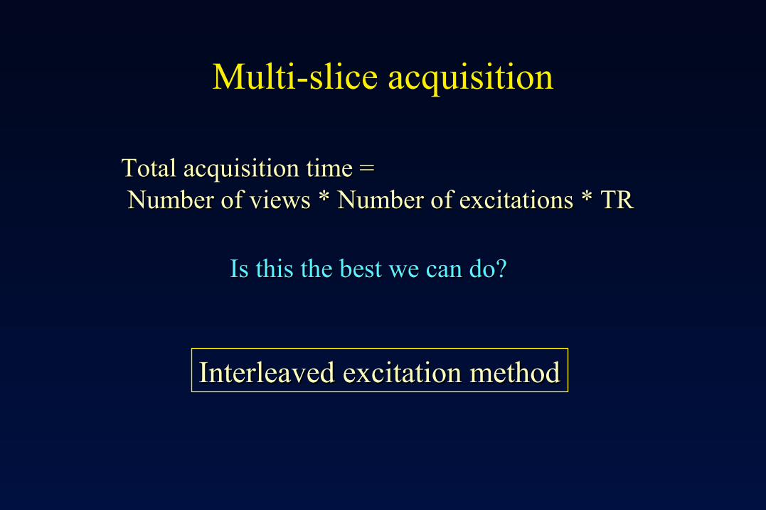
Multi-slice acquisition
Total acquisition time =Total acquisition time = Number of views * Number of excitations * TRNumber of views * Number of excitations * TR
Is this the best we can do?Is this the best we can do?
Interleaved excitation methodInterleaved excitation method
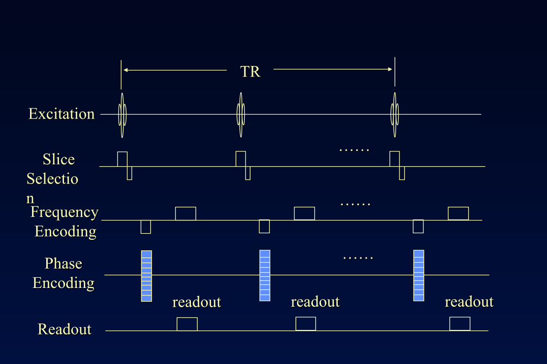
readoutreadout
ExcitationExcitation
SliceSliceSelectioSelectionnFrequencyFrequency EncodingEncoding
PhasePhase EncodingEncoding
ReadoutReadout
readoutreadout readoutreadout
…………
…………
…………
TRTR
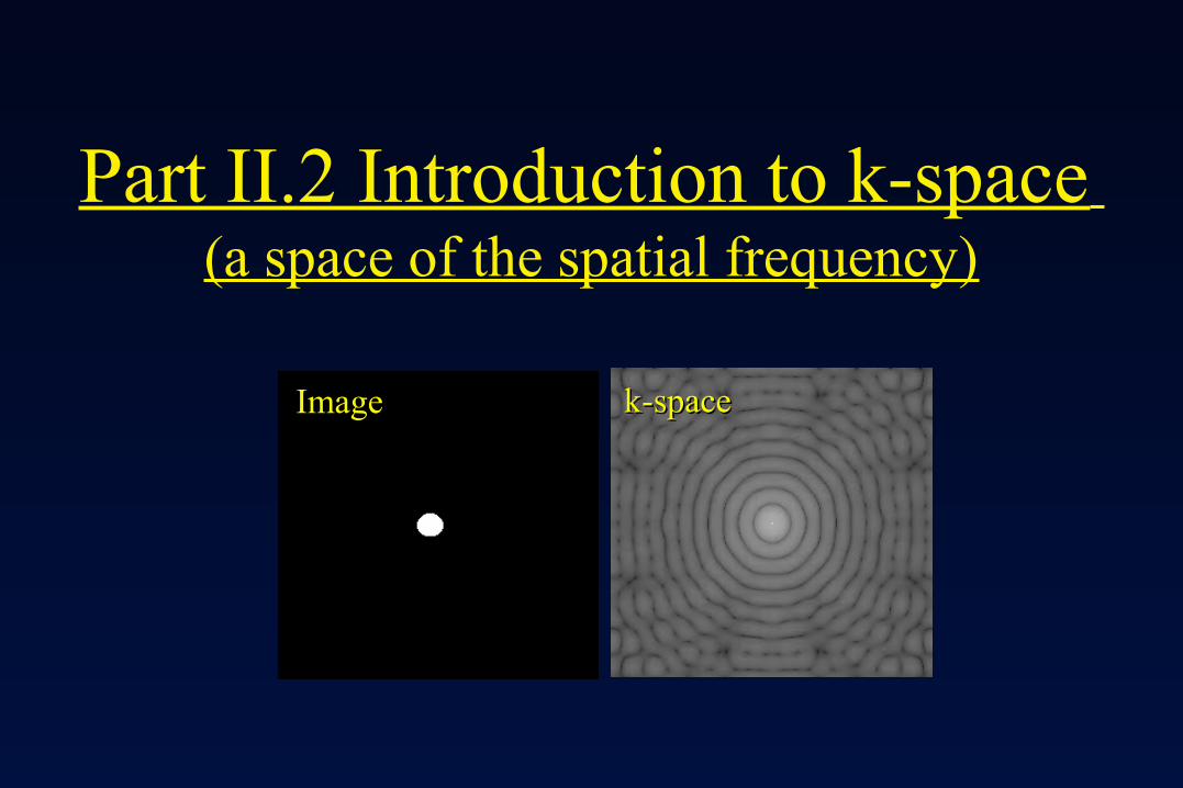
Part II.2 Introduction to k-space (a space of the spatial frequency)
ImageImage k-spacek-space
Acquired MR Signal
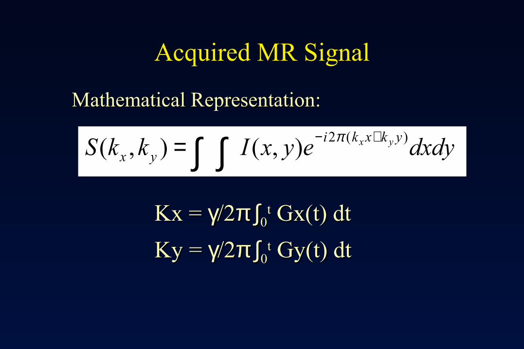
Mathematical Representation:Mathematical Representation:
dxdyeyxIkkS ykxkiyx
yx )(2),(),( +−∫∫= π
Kx = Kx = γγ/2/2π ∫π ∫00tt Gx(t) dtGx(t) dt
Ky = Ky = γγ/2/2π ∫π ∫00tt Gy(t) dtGy(t) dt
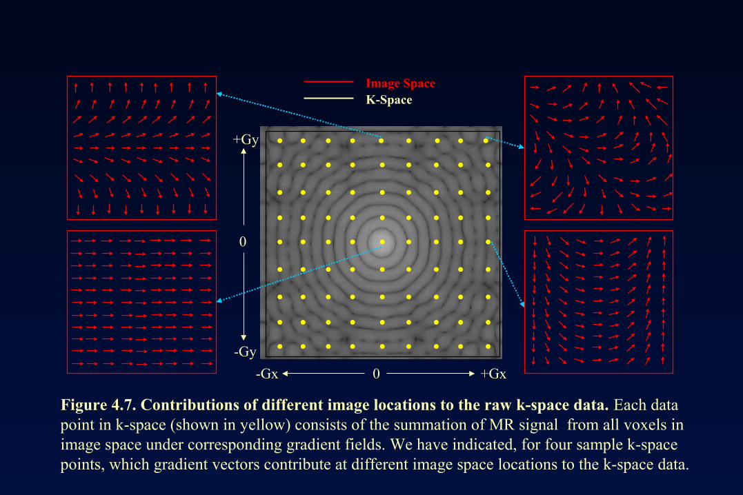
Figure 4.7. Contributions of different image locations to the raw k-space data. Each data point in k-space (shown in yellow) consists of the summation of MR signal from all voxels in image space under corresponding gradient fields. We have indicated, for four sample k-space points, which gradient vectors contribute at different image space locations to the k-space data.
..
.
..
.
.
.+Gx-Gx 0
0
+Gy
-Gy .
Image SpaceK-Space
..
.
..
.
.
..
..
.
..
.
.
..
..
.
..
.
.
..
..
.
..
.
.
..
..
.
..
.
.
..
..
.
..
.
.
..
..
.
..
.
.
..
..
.
..
.
.
..
Acquired MR Signal
dxdyeyxIkkS ykxkiyx
yx )(2),(),( +−∫∫= π
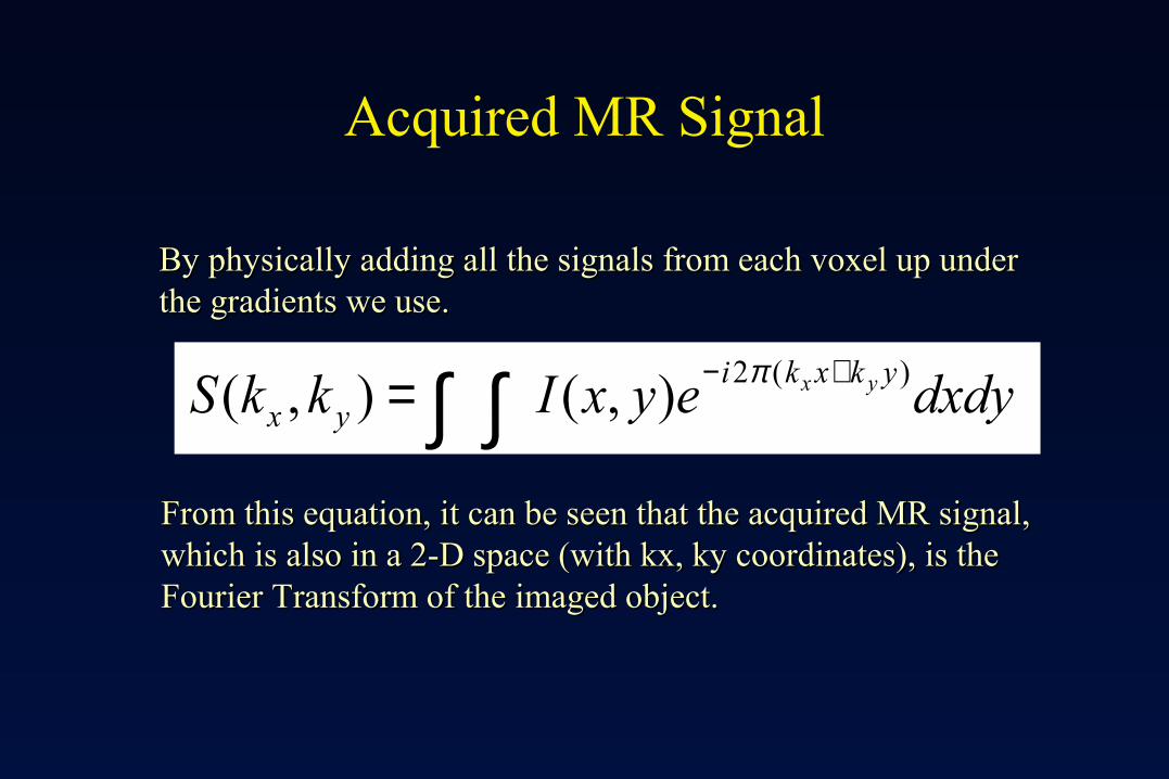
From this equation, it can be seen that the acquired MR signal,From this equation, it can be seen that the acquired MR signal,which is also in a 2-D space (with kx, ky coordinates), is the which is also in a 2-D space (with kx, ky coordinates), is the Fourier Transform of the imaged object.Fourier Transform of the imaged object.
By physically adding all the signals from each voxel up under By physically adding all the signals from each voxel up under the gradients we use.the gradients we use.
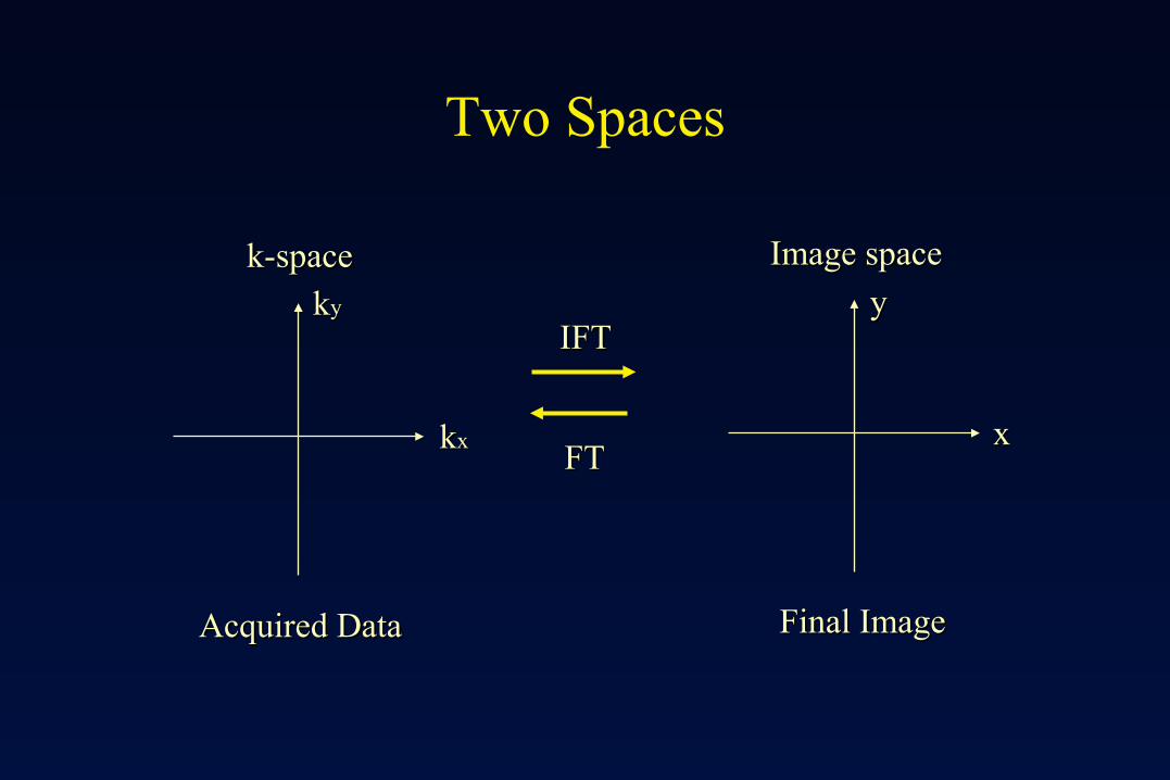
Two Spaces
FTFT
IFTIFT
k-spacek-space
kkxx
kkyy
Acquired DataAcquired Data
Image spaceImage space
xx
yy
Final ImageFinal Image
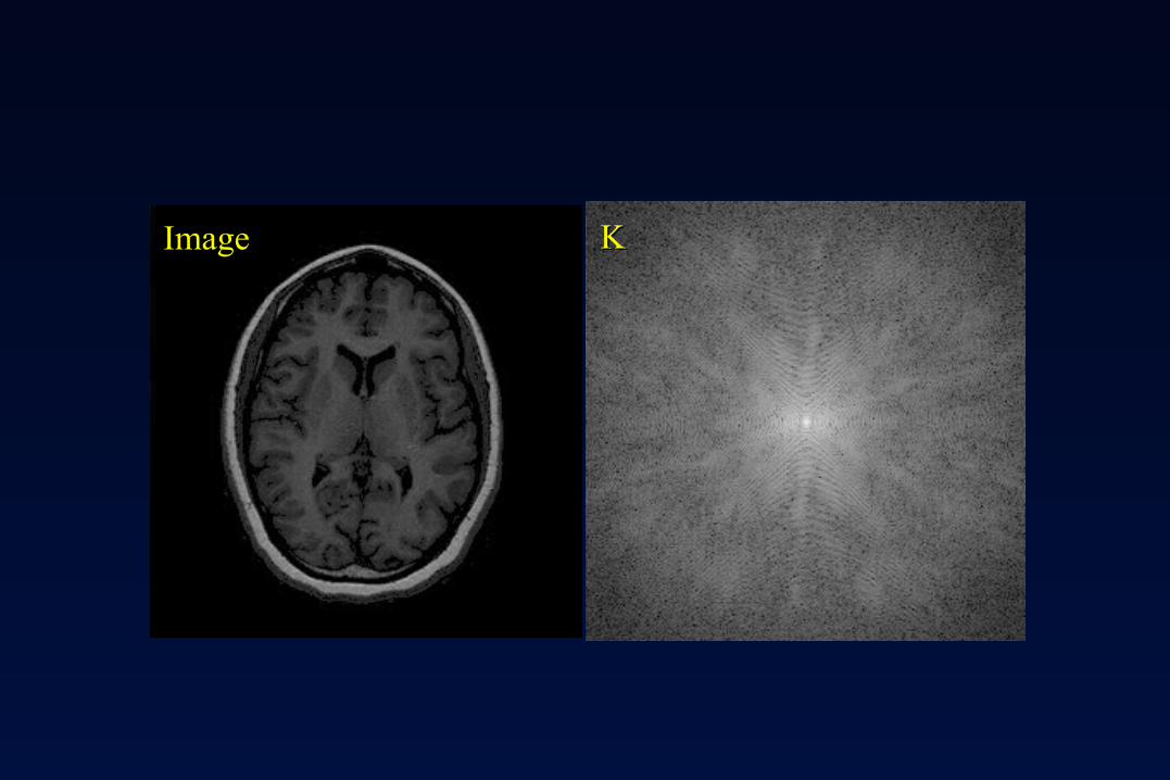
ImageImage KK
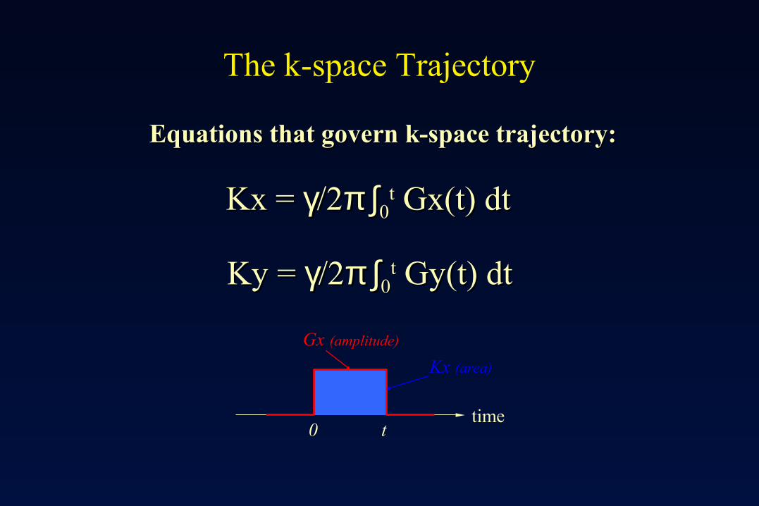
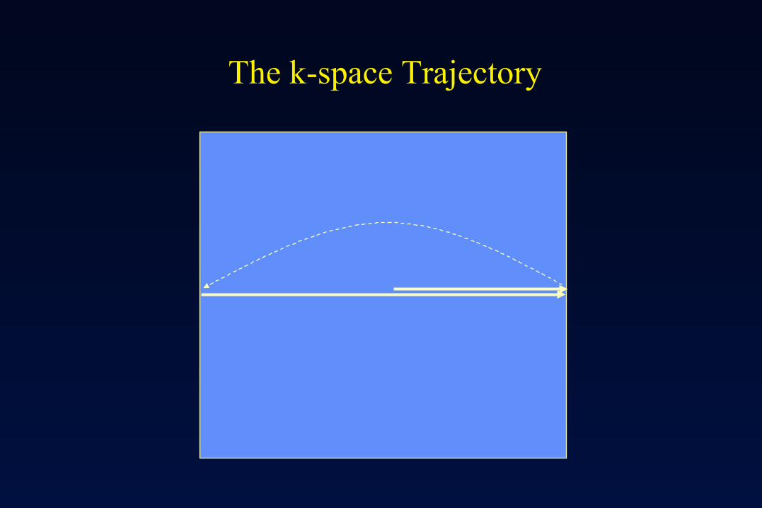
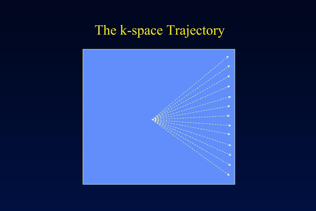
The k-space Trajectory
Kx = Kx = γγ/2/2π ∫π ∫00tt Gx(t) dtGx(t) dt
Ky = Ky = γγ/2/2π ∫π ∫00tt Gy(t) dtGy(t) dt
Equations that govern k-space trajectory:Equations that govern k-space trajectory:
time0 t
Gx (amplitude)
Kx (area)
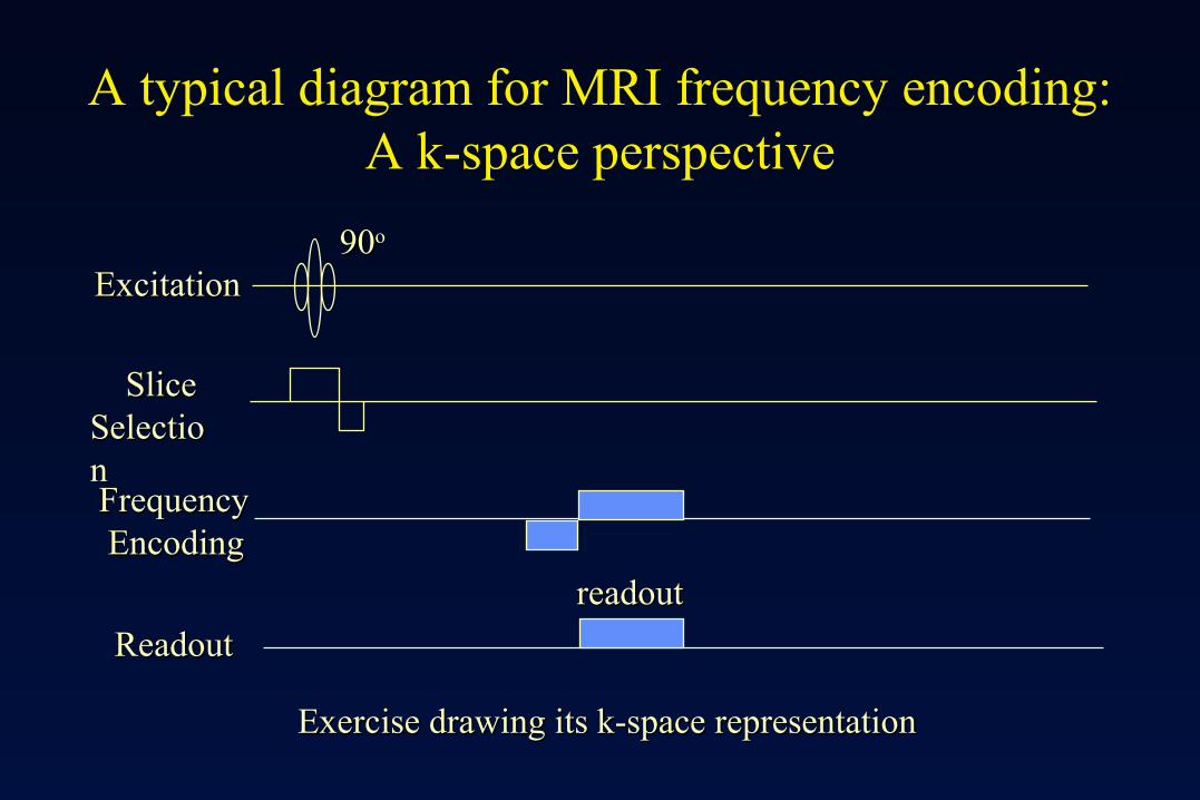
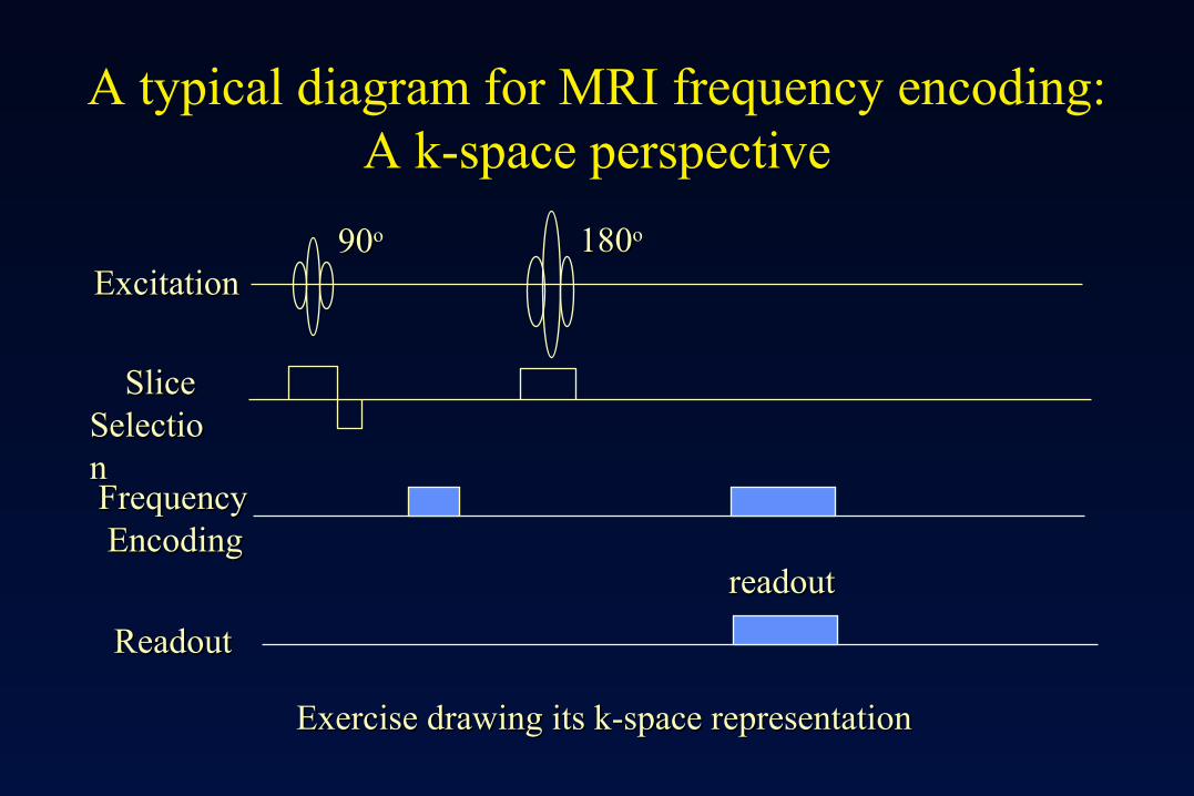
A typical diagram for MRI frequency encoding:A k-space perspective
readoutreadout
ExcitationExcitation
SliceSliceSelectioSelectionnFrequencyFrequency EncodingEncoding
ReadoutReadout
Exercise drawing its k-space representationExercise drawing its k-space representation
9090oo
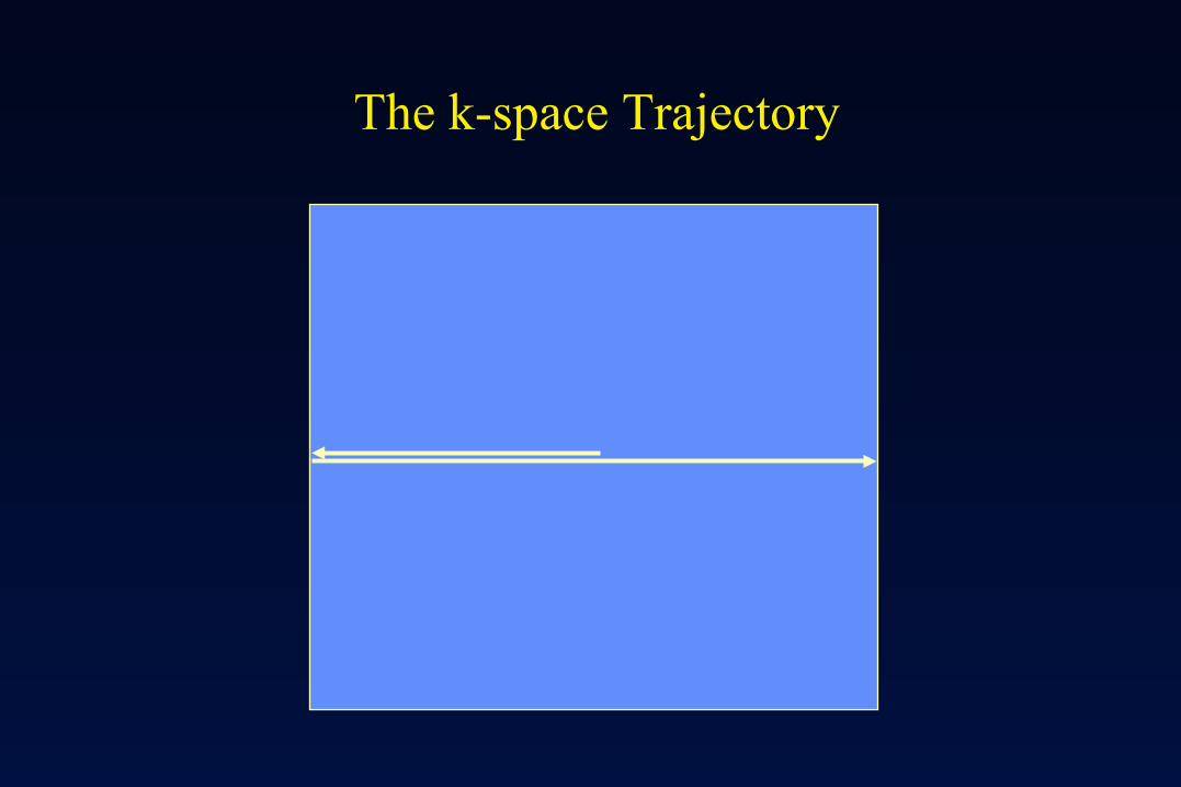
The k-space Trajectory
A typical diagram for MRI frequency encoding:A k-space perspective
readoutreadout
ExcitationExcitation
SliceSliceSelectioSelectionnFrequencyFrequency EncodingEncoding
ReadoutReadout
Exercise drawing its k-space representationExercise drawing its k-space representation
9090oo 180180oo
The k-space Trajectory
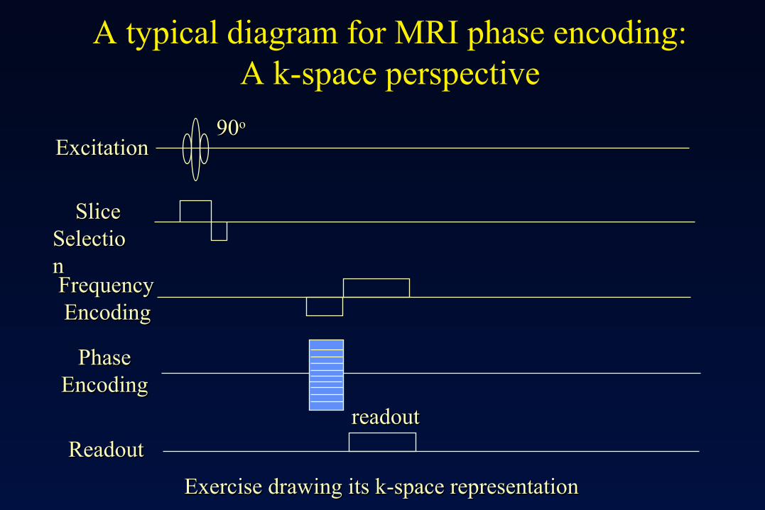
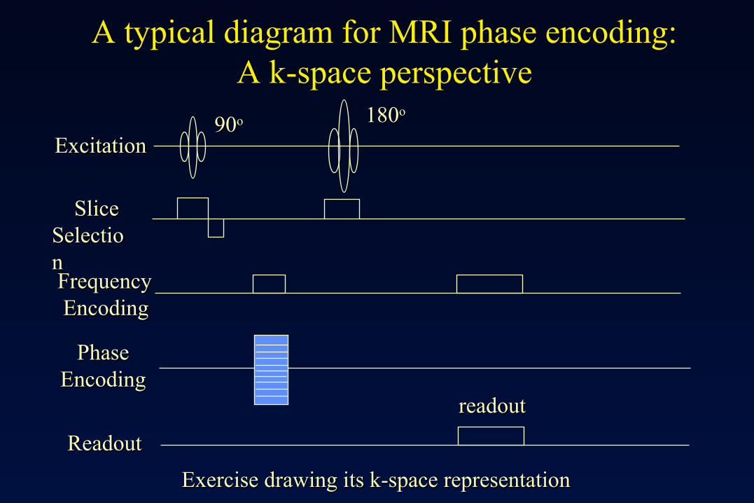
A typical diagram for MRI phase encoding:A k-space perspective
readoutreadout
ExcitationExcitation
SliceSliceSelectioSelectionnFrequencyFrequency EncodingEncoding
PhasePhase EncodingEncoding
ReadoutReadout
Exercise drawing its k-space representationExercise drawing its k-space representation
9090oo
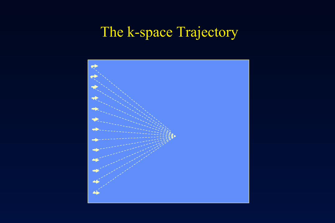
The k-space Trajectory
A typical diagram for MRI phase encoding:A k-space perspective
readoutreadout
ExcitationExcitation
SliceSliceSelectioSelectionnFrequencyFrequency EncodingEncoding
PhasePhase EncodingEncoding
ReadoutReadout
Exercise drawing its k-space representationExercise drawing its k-space representation
9090oo 180180oo
The k-space Trajectory
. . . . . . . . . .. . . . . . . . . .. . . . . . . . . .. . . . . . . . . .
. . . . . . . . . .. . . . . . . . . .. . . . . . . . . .. . . . . . . . . .. . . . . . . . . .. . . . . . . . . .. . . . . . . . . .. . . . . . . . . .. . . . . . . . . .. . . . . . . . . .
. . . . . . . . . .. . . . . . . . . .. . . . . . . . . .. . . . . . . . . .. . . . . . . . . .. . . . . . . . . .
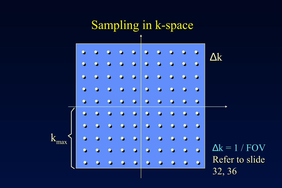
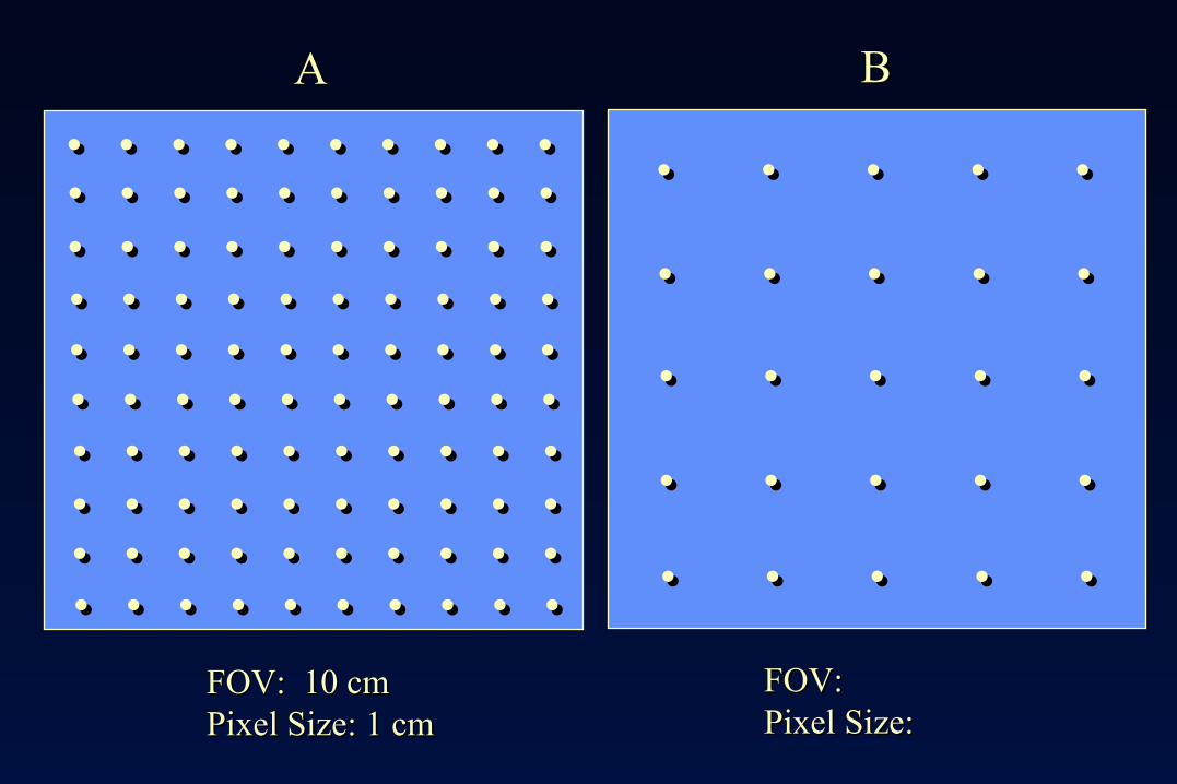
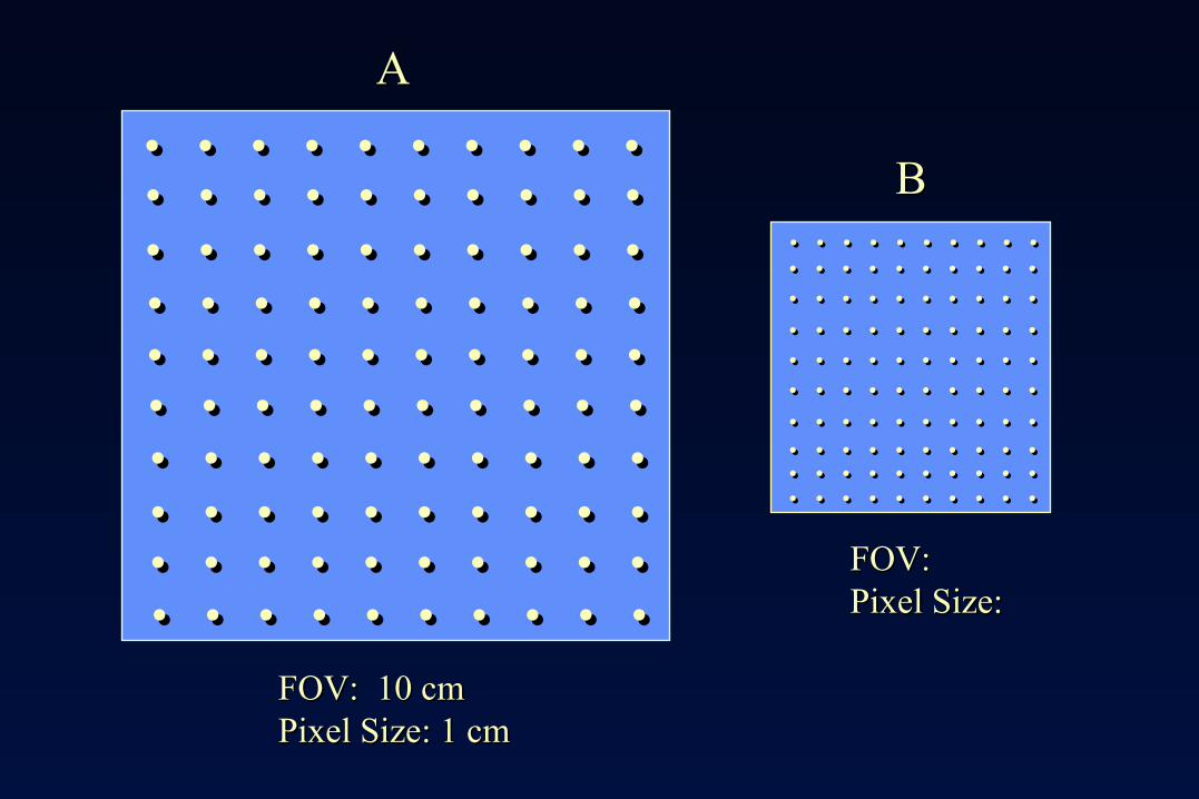
Sampling in k-spaceSampling in k-space
kkmaxmax
∆∆kk
∆∆k = 1 / FOVk = 1 / FOVRefer to slide Refer to slide 32, 3632, 36
. . . . . . . . . .. . . . . . . . . .. . . . . . . . . .. . . . . . . . . .
. . . . . . . . . .. . . . . . . . . .. . . . . . . . . .. . . . . . . . . .. . . . . . . . . .. . . . . . . . . .. . . . . . . . . .. . . . . . . . . .. . . . . . . . . .. . . . . . . . . .. . . . . . . . . .. . . . . . . . . .. . . . . . . . . .. . . . . . . . . .. . . . . . . . . .. . . . . . . . . .
. . . . .. . . . .. . . . .. . . . .. . . . .. . . . .. . . . .. . . . .. . . . .. . . . .
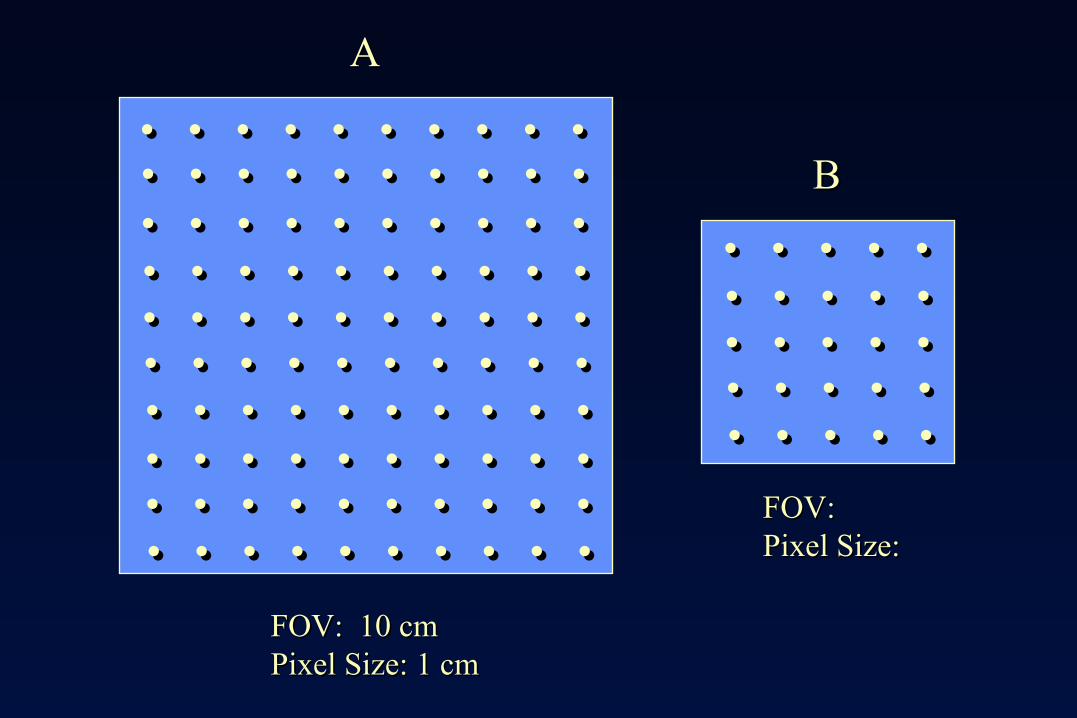
AA
BB
FOV: 10 cmFOV: 10 cmPixel Size: 1 cmPixel Size: 1 cm
FOV:FOV:Pixel Size:Pixel Size:
. . . . . . . . . .. . . . . . . . . .. . . . . . . . . .. . . . . . . . . .
. . . . . . . . . .. . . . . . . . . .. . . . . . . . . .. . . . . . . . . .. . . . . . . . . .. . . . . . . . . .. . . . . . . . . .. . . . . . . . . .. . . . . . . . . .. . . . . . . . . .. . . . . . . . . .. . . . . . . . . .. . . . . . . . . .. . . . . . . . . .. . . . . . . . . .. . . . . . . . . .
. . . . .. . . . . . . . . .. . . . . . . . . .. . . . . . . . . .. . . . . . . . . .. . . . .
AA BB
FOV: 10 cmFOV: 10 cmPixel Size: 1 cmPixel Size: 1 cm
FOV:FOV:Pixel Size:Pixel Size:
. . . . . . . . . .. . . . . . . . . .. . . . . . . . . .. . . . . . . . . .
. . . . . . . . . .. . . . . . . . . .. . . . . . . . . .. . . . . . . . . .. . . . . . . . . .. . . . . . . . . .. . . . . . . . . .. . . . . . . . . .. . . . . . . . . .. . . . . . . . . .. . . . . . . . . .. . . . . . . . . .. . . . . . . . . .. . . . . . . . . .. . . . . . . . . .. . . . . . . . . .
AA
BB. . . . . . . . . .. . . . . . . . . .. . . . . . . . . .. . . . . . . . . .. . . . . . . . . .. . . . . . . . . .. . . . . . . . . .. . . . . . . . . .. . . . . . . . . .. . . . . . . . . .. . . . . . . . . .. . . . . . . . . .. . . . . . . . . .. . . . . . . . . .. . . . . . . . . .. . . . . . . . . .. . . . . . . . . .. . . . . . . . . .. . . . . . . . . .. . . . . . . . . .
FOV: 10 cmFOV: 10 cmPixel Size: 1 cmPixel Size: 1 cm
FOV:FOV:Pixel Size:Pixel Size:
. . . . . . . . . .. . . . . . . . . .. . . . . . . . . .. . . . . . . . . .
. . . . . . . . . .. . . . . . . . . .. . . . . . . . . .. . . . . . . . . .. . . . . . . . . .. . . . . . . . . .. . . . . . . . . .. . . . . . . . . .. . . . . . . . . .. . . . . . . . . .. . . . . . . . . .. . . . . . . . . .. . . . . . . . . .. . . . . . . . . .. . . . . . . . . .. . . . . . . . . .
. . . . .. . . . .. . . . .. . . . .. . . . .. . . . .. . . . .. . . . .. . . . .. . . . .
. . . . .. . . . .. . . . .. . . . .. . . . .. . . . .. . . . .. . . . .. . . . .. . . . .
. . . . .. . . . .
. . . . .. . . . .
. . . . .. . . . .
. . . . .. . . . .
. . . . .. . . . .
. . . . .. . . . .
. . . . .. . . . .
. . . . .. . . . .
. . . . .. . . . .
. . . . .. . . . .
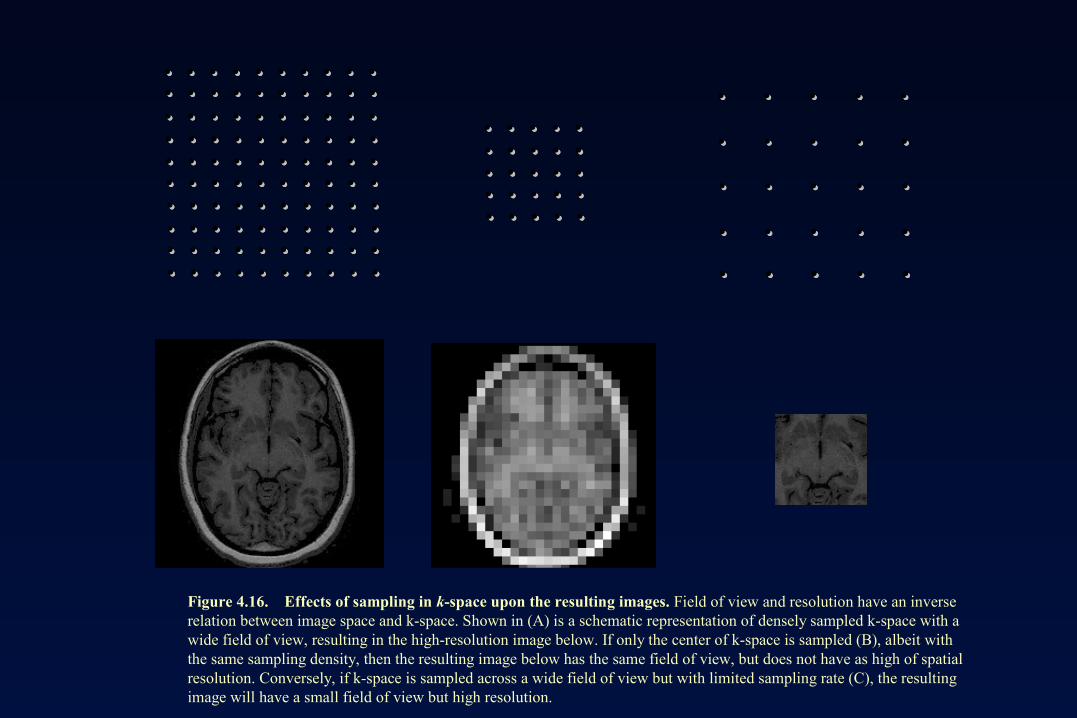
Figure 4.16. Effects of sampling in k-space upon the resulting images. Field of view and resolution have an inverse relation between image space and k-space. Shown in (A) is a schematic representation of densely sampled k-space with a wide field of view, resulting in the high-resolution image below. If only the center of k-space is sampled (B), albeit with the same sampling density, then the resulting image below has the same field of view, but does not have as high of spatial resolution. Conversely, if k-space is sampled across a wide field of view but with limited sampling rate (C), the resulting image will have a small field of view but high resolution.
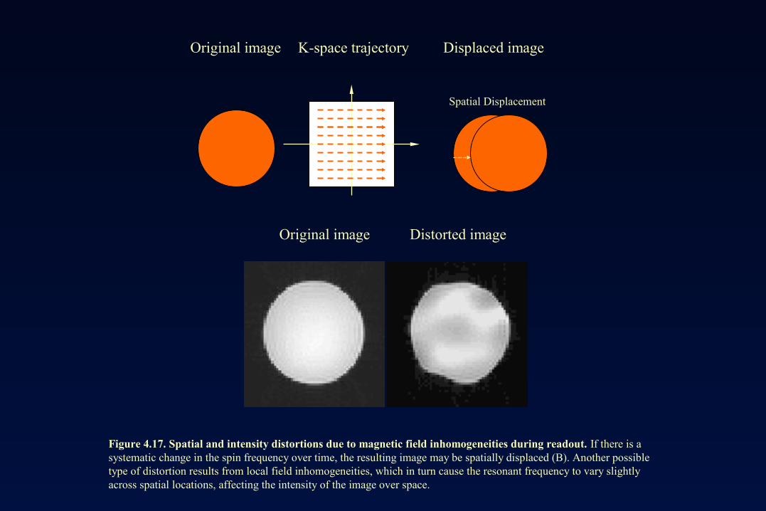
Spatial Displacement
Original image K-space trajectory Displaced image
Original image Distorted image
Figure 4.17. Spatial and intensity distortions due to magnetic field inhomogeneities during readout. If there is a systematic change in the spin frequency over time, the resulting image may be spatially displaced (B). Another possible type of distortion results from local field inhomogeneities, which in turn cause the resonant frequency to vary slightly across spatial locations, affecting the intensity of the image over space.
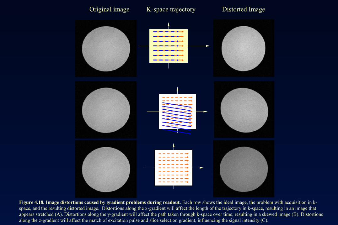
Figure 4.18. Image distortions caused by gradient problems during readout. Each row shows the ideal image, the problem with acquisition in k-space, and the resulting distorted image. Distortions along the x-gradient will affect the length of the trajectory in k-space, resulting in an image that appears stretched (A). Distortions along the y-gradient will affect the path taken through k-space over time, resulting in a skewed image (B). Distortions along the z-gradient will affect the match of excitation pulse and slice selection gradient, influencing the signal intensity (C).
Original image K-space trajectory Distorted Image