1I11111111111111111111111111111111111111111111111111111111111111 i

3 1176 00163 3172

CRS·1·80

THE USE OF SATELLITES IN ENVIRONMENTAL MONITORING

NASA-CR-162409 19800002442

OF COASTAL WATERS

W. Philpot and V. Klemas

..

THE USE OF SATELLITES IN ENVIRONHENTAL HONITORING

OF COASTAL l-lATERS

w. Philpot and V. K1emas College of Marine Studies University of Delaware Newark, Delaware 19711

eRS-I-SO

September .20, 1979 Final Report

NASA Grant NSG 1433

Prepared for

National Aeronautics & Space Administration Langley Research Center Hampton, Virginia 23665

7

..

TABLE OF CONTENTS

Page

I. Introduction 1

II. General Aspects of Environmental Monitoring 2

- major criteria in program d~~ign

- categories of monitoring programs

III. Remote Sensing of Water 6

3.1 Visible and near infrared region 8

3.1.1 Physical interactions 8

Volume interaction 8

Air-sea interface 17

Polarization 21

Atmospheric effects 21

3.1.2 System characteristics 26

Spectral characteristics 26

Radiometric sensitivity and dynamic range 27

Spatial resolution, swath width and coverage frequency 35

3.1.3 Visible sensors on satellites

3.2 Thermal infrared region

3.3 Microwave region

IV. The Role of Satellite Remote Sensing in Environmental Monitoring

4.1 Specific targets

4.1.1 Photosynthetic pigments

4.1.2 Iron-acid waste

4.1.3 Sewage sludge

4.2 General monitoring

V. Con.c1us ions

37

41

43

47

47

47

53

56

58

61

References

Appendix A: Landsat

Appendix B: Nimbus

Appendix C: Multispectral Resource Sampler

Appendix D: NOSS

Appendix E: Thermal Sensors

Appendix F: Microwave Sensors

Page

64

70

72

73

74

76

77

.,

I. Introduction

Satellite remote sensing is likely to play an important and very

special role in environmental monitoring in coastal waters. Satellite

systems are the only tools available which are capable of truly synoptic

coverage of the enormous areas requiring surveillance. Beyond the

obvious role of providing a synoptic view, the role of satellite remote

sensing is not easily defined. In the first place, the water parameters

which can be measured remotely are often only indirectly related to

measurements that would be made from ship. Shipboard measurements are

the standard against which remote measurements must be compared, and

which will probably never be supplanted by remote sensing, even though

ships cannot be expected to provide adequate coverage of the entire

coastal region. Secondly, the utility of satellite data for detection

and identification of pollutants will depend on the sensor characteristics

of the satellite systems (spectral bands, spectral and spatial resolution,

sensitivity and dynamic range). In some cases satellite data may be

adequate for positive identification of a specific pollutant, in other

cases the pollutant may be only marginally detectable or entirely

undetectable from the available satellite data. Thirdly, the coastal

regime is a dynamic system. Characteristic features of dumps or spills

will change relatively rapidly due to advection, diffusion, settling and

physical or chemical changes of the material. This temporal variability

will lead to stringent requirements for the temporal coverage needed for

different monitoring programs. Finally, the role of satellite remote

sensing in environmental monitoring will depend heavily on the specific

goals of the monitoring program.

The objective of this study is to evaluate the feasibility of using

2

satellites available during the 1978-1990 time period in an operational

system for monitoring the type, concentration, location, drift and

dispersion of pollutants in coastal waters.

II. General Aspects of Environmental Monitoring

"Environmental monitoring is the systematic collection and evaluation

of physical, chemical, biological and related data pertaining to environ­

mental quality, pollution sources, and other factors which influence, or

are influenced by environmental quality." (EPA, 1973). We, of course,

are concerned here only with the environmental monitoring of coastal and

estuarine waters and the role that remote sensing will play in this

task. As is suggested by the above definition, the monitoring task is

broader than the detection and identification of pollutants in water; it

also involves the determination of the nature of the unperturbed aquatic

environment and observation of long term trends in environmental quality.

In the discussions that follow, the word "pollution" will be used

frequently. We will define pollution as the presence of matter or

energy whose nature, location or quantity produces undesired environ­

mental effects (EPA, 1977). This definition includes such things as

heated water discharged from a power plant and undesireable plankton

blooms as well as oil spills and sewage sludge dumps. Likewise, the

term "pollution event" will be used to mean the occurence of a par­

ticular incident (e.g. an oil spill) or a set of circumstances (e.g. the

presence of the necessary physical, chemical and biological conditions

for an undesireable plankton bloom) which results in pollution of the

water.

Several very different types of monitoring programs can be developed.

3

The nature of the programs will depend primarily on three criteria:

1) Data requirements

Generally, the more narrow and specific the goals of the monitoring

effort, the simpler the data requirements. For instance, monitoring the

thermal effluent from one power plant is a relatively simple matter only

requiring measurements of temperature; monitoring the effect of the

thermal effluent on the area near the outfall is vastly more complex.

The quality of data will also vary. For instance, for some purposes it

may be necessary only to detect the presence of a pollutant while for

other purposes it may be necessary to establish the concentration and/or

distribution of the material.

2) Temporal constraints

Both data rate and the total period of data acquisition will vary

depending on the types of measurements being made, the time scales of

motion in the region being monitored and the goals of the monitoring

program. Another factor which must be considered is the time frame in

which the data is to be used. In cases where immediate action is

necessary, the information must be available as quickly as possible. As

an instance, when a large oil spill occurs, information about the

location and movement of the oil is needed quickly in order to direct

clean-up operations. At the other extreme are the long-term monitoring

programs where no fast response is expected.

3) Geographic area

An extremely important characteristic which must be considered in

designing a monitoring system is the physical size of the area which

must be monitored. If the area is small it may be feasible to have

permanent instrument installations, e.g. a thermistor array used to

4

monitor the hot water ~vastes from a pmver plant. For larger areas,

permanent installations are generally impractical and other means must

be found. It is in the monitoring of large areas that remote sensing is

most promising.

Hith these criteria in mind ~ve may identify several different

categories of environmental monitoring in coastal waters:

1) Fast response operations

In this category, the goal of monitoring is to provide early warning

of a pollution event so that protective and/or corrective measures may

be taken. This requires early detection of the pollutant and fast

information transfer. The requirement for early detection suggests that

monitoring must be either continual or very high frequency. Continual

monitoring is usually accomplished with permanent systems dedicated to

the monitoring of specific pollutants. This category may include both

point and non-point sources.

The requirement for early detection also implies that the infor­

mation about the pollution event must be made available to the respon­

sible agency as soon as possible after the event. Thus the data must be

available quickly and in a form which is readily usable.

2) Long-term local monitoring

This category involves the continual assessment of environmental

quality in particular areas. The purpose of this type of monitoring may

be 1) to evaluate long-term pollution levels, 2) to evaluate effectiveness

of pollution abatement efforts or 3) to identify potential problems.

Included here are such things as point sources, legal dumpsites, fishing

grounds or recreational areas. This category is similar to the first

category except that there is no requirement for real-time data. Data

5

should be available in a matter of weeks or a few months. The frequency

of data collection depends on the specific type of pollution and the

dynamics of the system being observed but long-term changes are most

important. The major defining characteristic though, is that only a

limited geographic area is being monitored.

3) Long-term regional monitoring

In this case interest is in the general environmental quality of

large regions over extended periods of time. The data collected in this

type of program will generally be used in setting pollution guidelines

(or evaluating the effect of existing programs) and in observing the

long-term trends in pollution levels and their effect on the ecosystem.

The geographic area covered will be large and the time scale for data

availability will be on the order of months or years.

4) Enforcement monitoring

Enforcement monitoring involves documenting violations of environ­

mental quality standards. Data in this category are generally collected

through intensive, short-term monitoring efforts and are focused on

detection of specific pollutants or specific effects of those pollutants.

5) Historical data aCquisition

Historical data refers to data which already exists, which in some

way relates to environmental monitoring problems.

The monitoring categories are intended to be quite general (except

for being restricted to the aquatic environment) and to include all

forms of monitoring. These are not "official" categories as outlined by

any monitoring agency. Rather, these categories are delineated by

characteristics which are relevant to remote sensing (nature of the

data, temporal constraints, geographic area) and they are presented here

6

in order to gain a better perspective of the role of remote sensing in

monitoring programs.

III. Remote Sensing of Hater

Some form of remote sensing is likely to be an important facet of

the data gathering effort for many environmental monitoring efforts.

Aerial photography and aircraft-mounted sensor systems have already been

used for many monitoring-style applications. However, in most instances

satellite remote sensing data has not figured very heavily in environ­

mental monitoring. To some extend this is due to the limited types of

data available and the fact that satellite data had not been proven to

be useful for this purpose. This is changing; satellite data has been

used in many studies of environmentally significant features in coastal

and estuarine waters. It has been shown possible to detect oil (Deutsch,

1977) iron-acid waste (Ohlhorst and Bahn, 1978; Klemas et al., 1978) and

suspended solids whether occurring naturally as sediments (Maul and

Gordon, 1975; Johnson, 1975) or deposited in the ocean by man (Johnson

et a1., 1977). There has even been some limited success with detection

of chlorophyll from space (Strong, 1978; Hovis and Clark, 1979; Jensen

et al., 1979).

Besides the detection of specific materials in ocean water, satellite

data can be used for observation of other water features which are

important in environmental monitoring. Circulation patterns have been

inferred from sediment patterns seen in Landsat data (K1emas et al.,

1974; Carlson, 1974) as well as from the temperature patterns apparent

in thermal imagery from the NOAA satellites (Halliwell, 1978). Satellite

data has even been found useful in inferring fish distribution and

7

abundance estimates (Kemmerer, 1979) and in observing the impacts of

land use on estuarine water quality (Hill, 1979).

Given this broad range of success it is reasonable to expect that

satellite data will become a standard part of many monitoring programs.

Certainly there are many advantages to satellite data: (1) The most

obvious of the advantages is the large area coverage - the synoptic

view. This is extremely important for monitoring in coastal waters

since the areas to be covered are enormous. While satellite data do not

replace direct measurements they remove the restriction to the very

limited point-by-point gathering of water quality information. The

conventional data base can be greatly expanded and extrapolated spatially.

(2) In those cases for which satellite data proves to be useful, the

data volume-to-cost ratio should be significantly higher than for surface­

based techniques (Alfoldi and Munday, 1977). The actual cost of using

satellite data in an operational system depends both on the data require­

ments and the type of analysis. As yet no thorough cost-benefit analysis

has been done evaluating an operational use of satellite data. In fact,

there are actually very few estimates of the costs involved in either

research or operational uses. Such evaluations are needed and should be

undertaken in the near future. (3) Another advantage to satellite data

is that it can be used to provide an historical perspective on the

environment. Data is available from the Landsat and NOAA satellites

dating from 1972 and 1970 respectively. This data may be used as base­

line information for observations of long-term environmental changes.

Satellite remote sensing is likely to play a very important role in

environmental monitoring. The possible applications will depend heavily

8

on the satellite and sensor characteristics. In this section we will

consider the general characteristics of satellite remote sensing systems,

the types of measurements each can make and the constraints inherent in

each system. There are three regions of the electromagnetic spectrum

which are useful for the remote sensing of water: the visible and near

infrared (.4 ~m to 3 ~m, the thermal infrared (3 ~m to 5 ~m; 8 ~m to 14

~m) and the microwave (0.1 cm to 100 cm). Each of these regions will be

considered separately.

3.1 Visible and near infrared region (.4 ~m - 3 ~m)

3.1.1 Physical interactions

The visible and near infrared regions are grouped together here

because of the overall similarity of the physical interactions of light

at these wavelengths with the water, and because the sensor character­

istics are similar and sometimes identical.

Volume Interactions

The visible region of the electromagnetic spectrum is unique in

that it allows information to be carried from below the ocean surface to

a remote sensor. In pure water (water from which all particulate matter

has been removed) the attenuation of light is dominated by the absorption

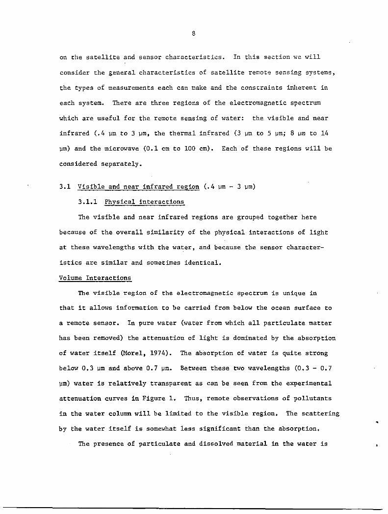
of water itself (Morel, 1974). The absorption of water is quite strong

below 0.3 ~m and above 0.7 ~m. Between these two wavelengths (0.3 - 0.7

~m) water is relatively transparent as can be seen from the experimental

attenuation curves in Figure 1. Thus, remote observations of pollutants

in the water column will be limited to the visible region. The scattering

by the water itself is somewhat less significant than the absorption.

The presence of particulate and dissolved material in the water is

9

10.0

I

.§. U

I-Z UJ

u 1.0 '"" u.. t u..

UJ I

0

f u z '" 0

~ ....

'. I-< '11·· => 0.1 z UJ l-I-< ... ~"! : .,

~ . : .....

< UJ ~

0.01

0.001 200 300 400 500 600 700 800

WAVELENGTH (nm)

............................................ Sawyer (1931) 310 - 650 nm

200 - 400 nm Dawson and Hulburt (1934) and Hulburt (1945)

400 - 700 nm

--------------- James and Birge {193BI 365 - BOO nm

.. _.-._._.-._._-_ .. Clark and James (1939) 365 - BOO nm

.......................................... Curcio and Petty (1951) 710 - 800 nm

• • • • • Lenoble and Saint-Guilly (1955) 220 - 400 nm

• • • •• • Armstrong and Boalch (1961a.b) 200 - 400 nm

•••••••• Sullivan (1963) 400 - 450 nm

580 - 790 nm

Figure 1. Attenuation curves for water in the near ultraviolet and visible parts of the spectrum. The spectral scattering coefficient, b, is shown for distilled water and sea water. Adapted from Smith and Tyler (1976).

10

generally far mc~e important to the penetration of light in water and

the intensity and color of the light scattered back in the direction of

the remote sensor. The strong scattering by the particulates (relatively

independent of wavelength) and absorption by all types of materials

(often significantly wavelength dependent) are the mechanisms which will

change the spectral reflectance characteristics of the water, and it is

the spectral reflectance characteristics of the water which are the most

important factor in the identification of substances in the water.

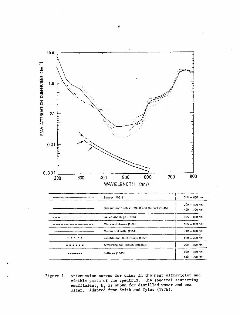
Typical variations in the apparent color of sea water are illus­

trated in Figure 2. These data representing a wide variety of water

types are selected from the spectral irradiance measurements reported by

Tyler and Smith (1970). The data in Figure 2 are spectra of the upwelling

irradiance measured at a depth of 5 meters except for the San Vincente

data which, because of the extreme turbidity of the water, was measured

at a depth of 1 meter. The curves have been normalized to the maximum

irradiance to facilitate comparison. The solar irradiance at the water

surface at three of the stations, also normalized to the maximum irradiance,

is also presented in Figure 2 in order to illustrate that the spectral

variations in the upwelling radiance are primarily due to differences in

the water masses and not because of spectral changes in illumination

conditions. Crater Lake water is "exceptionally free of contaminants of

any kind including chemical, planktonic or particulate contaminants"

(Tyler and Smith, 1970) and is about as close to pure water as can be

found anywhere in the world. Both the Gulf Stream and Tongue of the

Ocean are clear oceanic water types. The Gulf of California represents

coastal water while San Vincente, a man-made lake, represents water

11

A.

• 5 -. f."OOr:/ ~.. _ .. ;,# ,,~IJ

.; •• W ... ., ", ~"" .. ' . ..... ~

f

0".00

0.1 w u z B, « Q ~ 0:: 0::

0.1 " " W D

> " " " .- " « " " -l • UJ 0.01 •

" 0::: " " . " 0 . .

" 0

" "

0.001

,1, .S .6 .7

WAVELENGTH

Figure 2. a) Solar irradiance on the water surface.

b) Upwelling irradiance below the water surface. Depth is 5m for all stations except San Vincente which is for a depth of 1m.

All curves have been normalized to the maximum values. The data is taken from Tyler and Smith (1970).

Crater Lake Gulf Stream --------------­Tongue of the Ocean ••••••••••••• Gulf of California III I I III I I San Vincente 06000-0 0000 (

12

~vhich is "heavily contaminated ~vith pt:ytoplankton, zooplankton and

plankton decomposition products."

There certainly appears to be a sufficient range of spectral

variation in these examples for identifying water types. Unfortunately,

it is not merely the type of material present in the ~vater, but its

distribution in the water column that will affect the observed radiance

at the surface. The signal measured by a remote, passive, optical

system represents the integrated return from the entire water column.

The integration is weighted by the vertical distribution of optically

important materials in the water column. It is common to assume that

the water is vertically homogeneous, however this is often untrue. If a

pollutant is less dense or only slightly more dense than the water it

may remain near the water surface and not be distributed evenly throughout

the column. When the material does sink, a pycnocline or thermocline

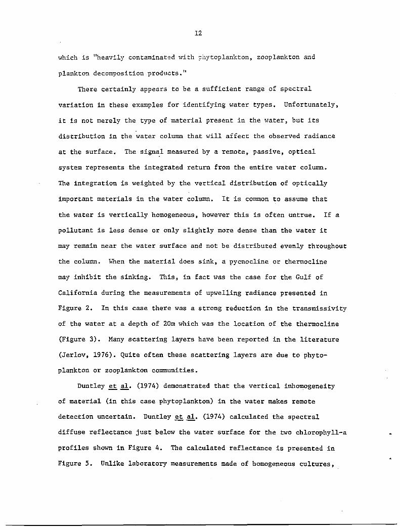
may inhibit the sinking. This, in fact was the case for the Gulf of

California during the measurements of upwelling radiance presented in

Figure 2. In this case there was a strong reduction in the transmissivity

of the water at a depth of 20m which was the location of the thermocline

(Figure 3). Many scattering layers have been reported in the literature

(Jerlov, 1976). Quite often these scattering layers are due to phyto­

plankton or zooplankton communities.

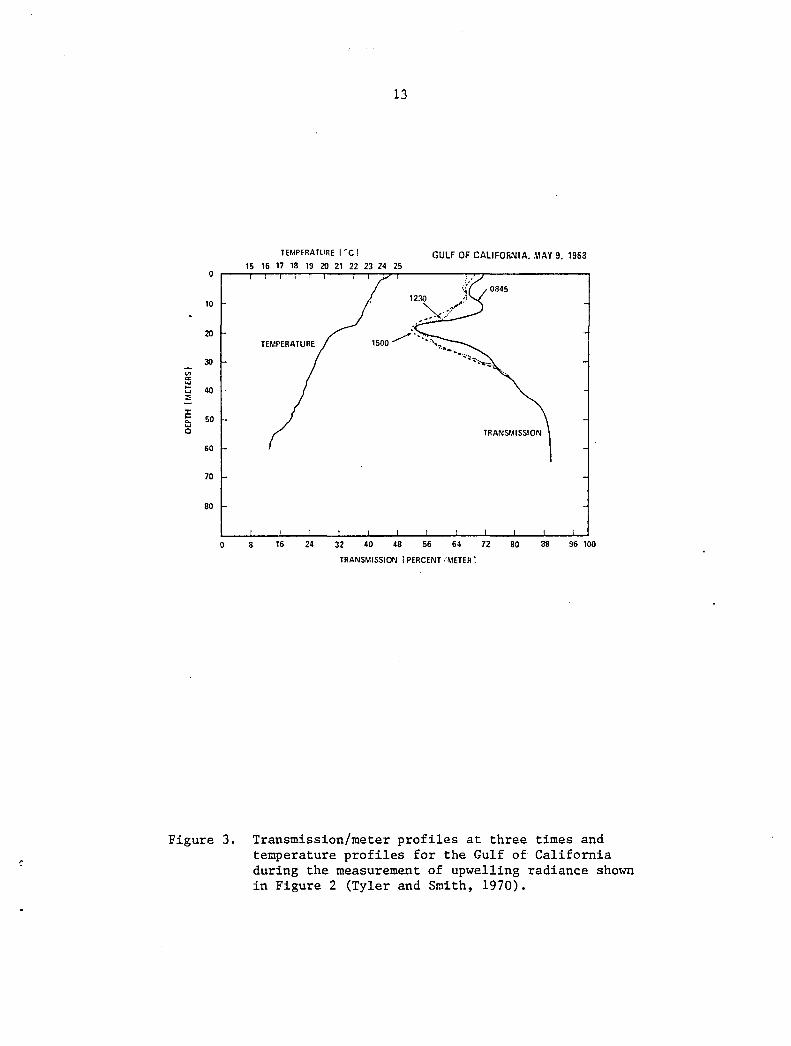
Duntley et al. (1974) demonstrated that the vertical inhomogeneity

of material (in this case phytoplankton) in the water makes remote

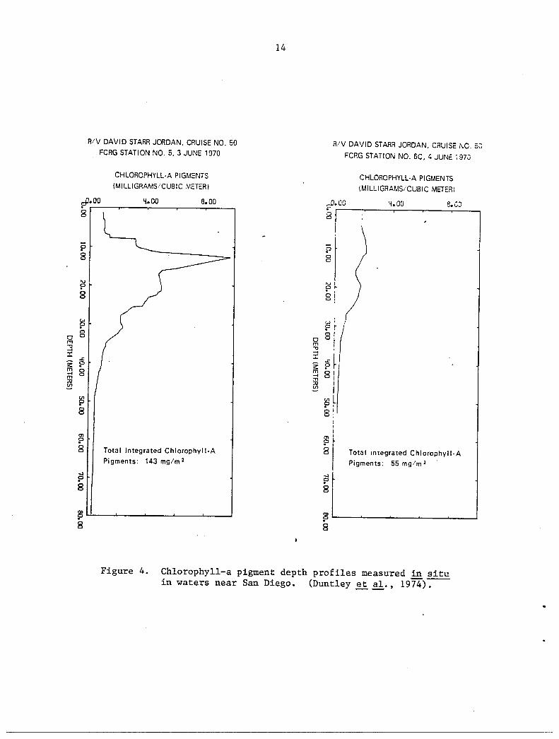
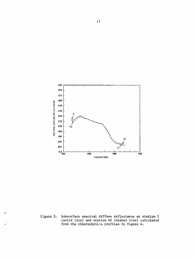
detection uncertain. Duntley et al. (1974) calculated the spectral

diffuse reflectance just below the water surface for the two chlorophyll-a

profiles shown in Figure 4. The calculated reflectance is presented in

Figure 5. Unlike laboratory measurements made of homogeneous cultures,

13

TEMPERA TURE I °c 1 GULF OF CALlFOR."lIA. MAY 9. 1968 15 16 17 18 19 20 21 22 23 24 25

0 :: .. ' "1 0845

10 1230 "

... ;,..:.:?,.... .. 20

1500,..........·····" 0':". .. -

30 VI a: "" ... 40 "" ::;;

~ 50 ... a 60

70

80

o 8 16 24 32 40 48 56 64 72 80 96 100

TRANSMISSION I PERCENT (METER I

Figure 3. Transmission/meter profiles at three times and temperature profiles for the Gulf of California during the measurement of upwelling radiance shown in Figure 2 (Tyler and Smith, 1970).

0 m "'0 -i ::c ;: m -i m ::D

!:!2

RN DAVID STARR JORDAN. CRUISE NO. 50

FCRG STATION NO.5. 3 JUNE 1970

CHLOROPHYLL-A PIGMENTS

(MILLIGRAMS/CUBIC METER)

14

RN DAVID SiARR JORDAN. CRUISe ;\0. 5;;

FCRG STATION NO. 6C. 4 JUNe ,97;)

CHLOROPHYLL-A PIGMENTS

(MILLIGRAMS/CUBIC METER)

~.oo 'i. 00 8.00 't.DO 8.CO co o

? 8

I\.J

? 8

? 0 0

J:;

? 0 0

P 8

'" ? 0 0

..... ? 8

Q)

? 8

Total Integrated Chlorophyll-A

Pigments: 143 mg/m 2

'" o • I

01 0,

..... ? 8

Total Integrared Chlorophyll-A

Pigments: 55 mg/m 2

pL....--'--_---' ____ ---' __ --" __ -J

8

Figure 4. Chlorophyll-a pigment depth profiles measured in situ in waters near San Diego. (Duntley et al., 1974).

.026

.024

.022

UJ .020 u z

.018 <{ ..... u UJ .016 ...J U-

S UJ a:

.014 , UJ

':S u.. .012 ,/ u- ! Ci ...J .010 6C <{ a: ..... .008 u w Cl. U) .006

.004

.002

0.0 400

15

/..-~

500

NANOMETERS

\ 6C

~--j r S

600 700

Figure 5. Subsurface spectral diffuse reflectance at station 5 ·(solid line) and station 6C (dashed line) calculated from the chlorophyll-a profiles in Figure 4.

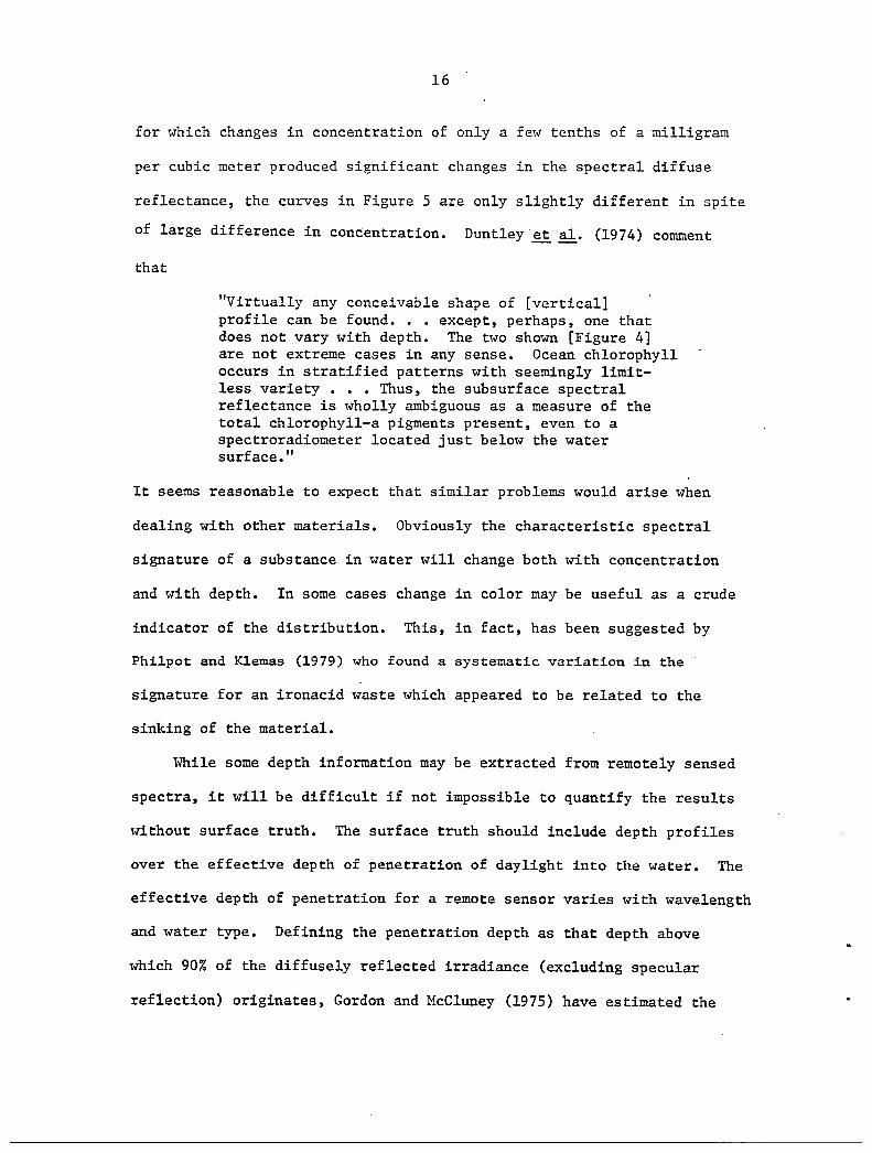
16

for which changes in concentration of only a fffiv tenths of a milligram

per cubic meter produced significant changes in the spectral diffuse

reflectance, the curves in Figure 5 are only slightly different in spite

of large difference in concentration. Duntley et ale (1974) comment

that

"Virtually any conceivable shape of [vertical] profile can be found ••• except, perhaps, one that does not vary with depth. The two shown [Figure 4] are not extreme cases in any sense. Ocean chlorophyll occurs in stratified patterns lvith seemingly limit­less variety ••• Thus, the subsurface spectral reflectance is wholly ambiguous as a measure of the total chlorophyll-a pigments present, even to a spectroradiometer located just below the water surface."

It seems reasonable to expect that similar problems would arise when

dealing with other materials. Obviously the characteristic spectral

signature of a substance in water will change both with concentration

and with depth. In some cases change in color may be useful as a crude

indicator of the distribution. This, in fact, has been suggested by

Philpot and Klemas (1979) who found a systematic variation in the

signature for an ironacid waste which appeared to be related to the

sinking of the material.

While some depth information may be extracted from remotely sensed

spectra, it will be difficult if not impossible to quantify the results

without surface truth. The surface truth should include depth profiles

over the effective depth of penetration of daylight into the water. The

effective depth of penetration for a remote sensor varies with wavelength

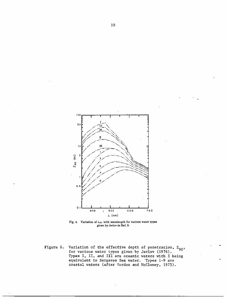
and water type. Defining the penetration depth as that depth above

which 90% of the diffusely reflected irradiance (excluding specular

reflection) originates, Gordon and McCluney (1975) have estimated the

17

penetration ciepth for Jerlov's water types. Their results are shown in

Figure 6. Jer1ov's water types (Jer1ov, 1976) would correspond to the

base waters in which one might look for pollution. The spectral signature

relative to the base water signature may be related to concentration and

depth distribution of a pollutant (Philpot and K1emas, 1979), but quan­

titative results will at least require identification of the base water.

In general, while it may very well be possible to detect the presence

of a pollutant in water by passive, optical remote sensing, quantification

will usually require surface support. The situation (for satellite

remote sensing) is only likely to improve if active (lidar) systems are

found to be feasible for satellite. Lidar systems are presently under

development for oceanographic applications (Collis and Russell, 1976;

Mumo1a et a1., 1973; Leonard ~ a1., 1979). However, 1idar systems are

still very much in the research stage even for aircraft, and problems

with power and eye-safety requirements will seriously hamper extension

of this technique to satellite based observations.

Air-sea interface

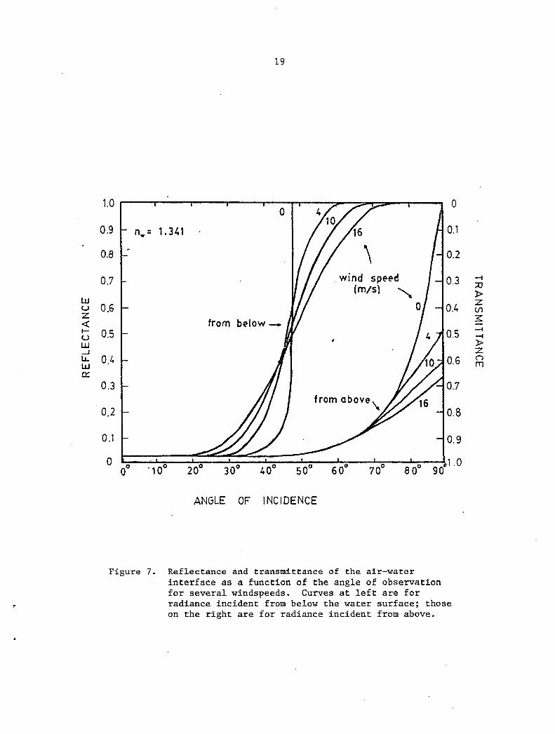
The air-sea interface affects the remotely sensed radiance in two

ways (1) it reduces the upwelling radiance from below the surface by

internal reflection and (2) it reflects sunlight and/or skylight into

the field of view of the sensor. Gordon (1969) has calculated the

reflectance coefficients for different angles of view and for a variety

of windspeeds. These are presented in Figure 7. According to Figure 7

the internal reflection will be less than 0.03 for most wind speeds, for

observation angles of ~30° in air. (This corresponds to an observation

angle in water of ~22°.) The specular reflection is easily less than

0.03 out beyond observation angles of 30°.

18

IOO~--~--~----~---r--~r---,----j

0.1 '--__ ....... __ --L _________ ....... __ --' ____ -'-__ ....

400 500 coo 100

A (nm)

Fig. 4. Variation of Z90 with wavelength for various water types given by Jerlov in Ref. 9.

Figure 6. Variation of the effective depth of penetration, 290

, for various water types given by Jerlov (1976). Types I, II, and III are oceanic waters with I being equivalent to Sargasso Sea water. 'Types 1-9 are coastal waters (after Gordon and McCluney, 1975).

w u z <{ t-u w .J LL lLJ 0::

19

1.0 a 0

0.9 n = 1. 341 0.1 w

0.8 \ 0.2

0.7 . wind speed 0.3 (m/s)

"" 0.6 0 0.4 from below_

0.5 0.5

0.4 0.6

0.3 0.7

0.2 from above\

0.8

0.1 0.9

0 Cl1.0 0° '10° 20° 30° 40° 50° 60° 70° 80° 90

ANGLE OF INCIDENCE

Figure 7. Reflectance and transmittance of the air-water interface as a function of the angle of observation for several windspeeds. Curves at left are for radiance incident from below the water surface; those on the right are for radiance incident from above.

-I ;0

l> z (J)

3: -I -I » z (')

rn

20

For most observation-angles of importance for satellite remote

sensing, the loss to internal reflection will not be a significant loss

due to refraction. The refraction effect is described by Austin, (1974).

"The flux contained in a small solid angle, Qw below the surface will be

2 spread into a larger solid angle, Qa = n Q, above the surface. There­w

fore, a radiance emerging from the water surface will be decreased

further by the factor 1/n2 or 0.555 by virtue of refraction alone." The

total reduction in radiance upon crossing the air-water interface will

be ~ 50%.

The above discussion refers to water surfaces which are free of

contaminants. Surface contaminants can change the reflectance charac-

teristics of the sea surface. Surface films of one sort or another are

a very common feature on natural waters. These films may be naturally

occurring organic slicks produced by marine phytoplankton (Wilson and

Collier, 1972), by fish, or they may be the result of oil spills.

Natural slicks are usually only monomolecular layers, less than a wave-

length of light in thickness. Oil slicks from oil spills, on the other

hand, are frequently thick enough to cause visible interference colors

(Cox, 1974). These slicks may change the reflectance characteristics of

the water surface either by changing the sea surface roughness due to

the change in surface tension or by a direct change in the reflection

coefficient. If the index of refraction of the slick is greater than

water - the usual case - then the reflectance will exceed that of water

alone. Cox and Munk (1956) estimated that the reflection coefficient

will increase by ~ 50% at normal incidence and less at other angles.

Measurements by Horvath et ale (1971) indicate that the increase in

reflectance is somewhat greater. In any case, surface slicks are often

detectable by passive, optical remote sensing.

21

Slicks are not the only surface contami~ents. Detritus and living

biological material will also be present on the water surface at times.

In most cases, the relatively high reflectance from these surface materials

relative to water makes them readily detectable. This is especially

true for the near ultraviolet and infrared regions. Virtually useless

for detection of volume characteristics, the ultraviolet infrared reflectance

can be an invaluable aid for detecting oi~ (Horvath et al., 1971; White

and Breslau, 1978) or phytoplankton at the water surface (Bressette and

Lear, 1973)-.

Polarization

The use of polarization can, at least theoretically, aid in the

remote sensing of water properties. At Brewster's angle, which for

water is 53.3° (observation angle in air), the specular reflectance from

a flat ocean is perfectly polarized. A remote sensor viewing at this

angle may either reduce the subsurface radiance by half while accepting

all the specularly reflected radiance - this is a useful method for

observing surface features (Horvath et al., 1971) or reject the specular --component entirely in order to enhance the subsurface component.

Unfortunately, as Austin (1974) points out at Brewster's angle, "the air

mass is increased to 1.67, which may severely increase problems associated

with the atmospheric transmittance and path radiance in a significant

number of instances. Additionally, the introduction of the polarizer

must reduce the desired subsurface water signal by at least a factor of

two and this may prove detrimental "

Atmospheric effects

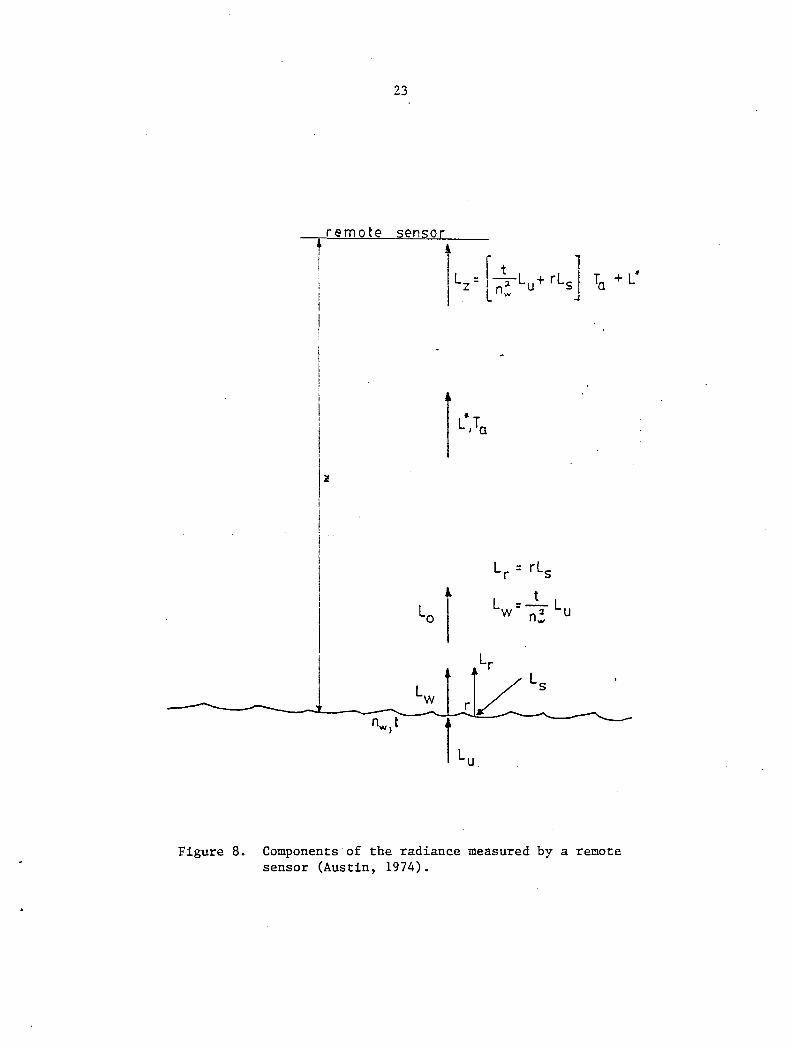
The radiance measured by a remote sensor is composed of several

components. These components are illustrated in Figure 8. The components

are as follows:

22

L = up_veIling radiance immediately below the water surface. u

L = upwelling radiance immediately above the water surface. w 2 = (tin ) L w u

L = sky radiance from that part of the sky ~vhich will be the s

source of specular reflectance seen by the remote sensor.

L = specularly reflected sky radiance = r L • r s

* L = path radiance, i.e. the radiance at the remote sensor due

entirely to the atmospheric scattering of sunlight and

skylight.

* L = (L + L ) T + L = radiance at the remote sensor. z w r a

r = reflectance of the air-water interface.

t = transmittance of the air-water interface.

T = atmospheric transmittance. a

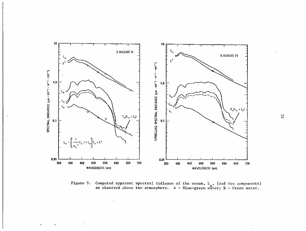
The various relative contributions to the satellite measured

radiance are illustrated in Figure 9 for two different water masses

(Austin, 1974). These curves are based on in situ reflectance measure----ments and on atmospheric transmittance measurements. They are fairly

typical for "clear" days and for clear coastal water types. The four

* circled points on the L and L curves for the 3 August data are values r

computed from shore station measurements.

The differences in color between the two water types is quite

evident in the radiance immediately above the water surface, L. Even w

after the addition of the specu1arly reflected skylight and degradation

due to atmospheric losses the major characteristics of the water color

are still quite apparent (see the curves marked T (L + L). However, a w r

* the signal measured at the satellite includes the path radiance, L ,

23

remote sensor

I : I I

i I Iz I

Lo

Lw

n ..... ,t

Lr : rLs

i t LW =-2 Lu

n ...

Lr

r~ Ls

k

T + L" a

Figure 8. Components of the radiance measured by a remote sensor (Austin, 1974).

I E c

I iii

I' §

~ ~ w u z ~ 0 « a: ...J

~ I-u w Q. II)

10 I 10

3 AUGUST 71 ~ f Lz

~~ 5 AUGUST 71

L* -" --....'" J I L·

I

~

I

lii

1.0 N

I 1.0 5

Lu ~ ~ w r Lu

Lw u

Lr

z « a ~ Lw « a: ...J Lr

0.1 T p(L,. t Lr) ~

~

"'~ I u ~ 0.1 II)

"-." CJ z :3 w

Lz~[_I_L trLJT tL" '\.....

il: 2 u d La

;:)

nw

0.01 1'----:~~:---.-.:L--L----'L----iL--.-.J 350 500 700

0.01 I 1. __ -,-_~

350 400 450 500 400 550 600 650 450 550 600 650 700

WAVELENGTH (nm) WAVELENGTH (nm)

Figure 9. Computed apparent spectral radiance of the ocean, L , (and its components) z as observed above the atmosphere. A - Blue-green water; B - Green water.

N .p-

25

which is nearly an order of magnitude greater than the transmitted

signal. In the examples sho,.u, the transmitted signal was never more

than about 20% of the path radiance and the spectral differences of the

total radiances measured at the satellite, L , are greatly reduced. z

Path radiance is the single most significant problem in remote

sensing in the visible region. It will vary greatly in both time and

space and may, at various times, be either significantly smaller or

greater than in the examples in Figure 9. There are basically two

approaches to dealing with the path radiance problem. The simplest,

most direct and, in many ways, most appealing approach is to emphasize

the relative changes in the spectra. This can be done by using ratios

of two or more bands (Arvesen ~ al., 1971; Curran, 1972) or by comparing

the spectra obtained from immediately adjacent areas (Clarke and Ewing,

1974; Philpot and Klemas, 1979), or by using some normalizing procedure

which will highlight the subtle changes in the spectra (Mueller, 1976).

The other approach is to measure or calculate the path radiance and

subtract it from the measured signal. This approach is frought with

difficulties. The determination of the path radiance must be quite

accurate since small changes in the path radiance can, and often do,

cause changes in the apparent radiance. Inaccurate determinations of

the path radiance will only introduce further anomalies in the apparent

radiance.

There is an awesome array of techniques proposed for determining

the path radiance. We will not attempt to describe or even to list

these methods here. It is an extremely important facet of optical

remote sensing and is an essential prerequisite if the full potential of

26

optical remote sensing is to be realized. It is also an extremely

difficult problem and is likely to be with us for some time.

3.1.2 System characteristics

In this section we will consider some of the characteristics of

remote sensing systems which will affect the utility of the system for

the various monitoring tasks.

Spectral characteristics

The question of the position, bandwidth and number of spectral

bands needed for the remote sensing of ocean color is not yet resolved.

The preferred spectral bands will vary depending on the particular

target (chlorophyll, sediment, oil, etc.) and may also vary with the

base water in or on which the target substance appears. Only general

spectral characteristics of ocean color will be presented here. Dis­

cussion of specific bands will be left for section IV.

The spectral characteristics of substances in the water will always

be masked to some extent by the absorption and scattering characteristics

of the water itself. The absorption and scattering effects of water

were described earlier. A more complete and excellent discussion of

this topic is provided by Morel (1974). One characteristic which has

important implications for remote sensing is that the absorption and

scattering effects of water are broadband, phenomena; there is little

fine structure. This is most explicitly demonstrated by the research

of Drummeter and Knestrick (1967) who found no narrow absorption bands

of any significance in water. This implies that it may not be necessary

(or even advantageous) to use extremely narrow bandwidths for most

observations of ocean color.

27

Some insight into the number of bands necessary has been provided

by Mueller's (1976) study of ocean color at 31 stations off the Oregon

coast. Mueller measured the complete water color spectra betw·een 420

and 700nm at a resolution of Snm to 7nm. Using characteristic vector

analysis, Mueller found that 99% of the variance in the normalized

reflectance could be accounted for by only four characteristic vectors.

In principle, then, one might need only five carefully chosen wavebands

to reproduce the essential variational features of the observed spectra:

one for each characteristic vector and one for the mea~ spectrum. Of

course, these spectra did not include observations of any of the more

common pollutants. Thus more than five bands may be needed for pollution

monitoring systems. In particular, Mueller (1979) notes that a fifth

characteristic vector is required to account for the spectra of iron­

acid waste.

Mueller (1979) also explored the effect of widening the bandwidth.

If, as suggested above, the spectral variations are truly broadband,

then Snm bandwidth may not be necessary. Mueller found that increasing

the bandwidth to more than about 20nm degrades the informational content

of the spectra. This implies that 20nm may be the optimal bandwidth for

remote sensing purposes; any wider and the information content will be

reduced, narrower and the total power in the received signal will be

reduced.

Radiometric sensitivity and dynamic range

It was stated above that one of the most important aspects of ocean

color analysis is the observation of subtle variations in the spectra.

This implies that the sensors must be quite sensitive. Yet the sensors

must be capable of this high sensitivity over a broad enough dynamic

..

28

range for the data to be usable under very hazy conditions, when path

radiance is very high, as ~vell as on clear days •

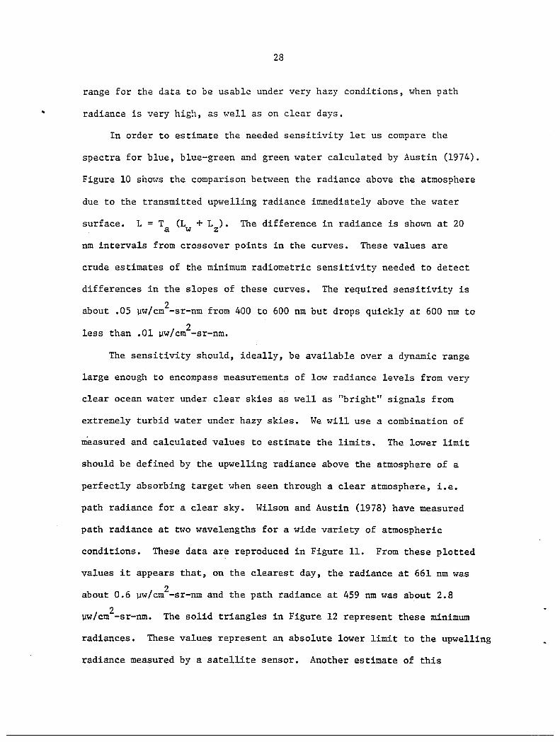
In order to estimate the needed sensitivity let us compare the

spectra for blue, blue-green and green water calculated by Austin (1974).

Figure 10 shows the comparison between the radiance above the atmosphere

due to the transmitted upwelling radiance immediately above the water

surface. L = T (L + L). The difference in radiance is shown at 20 a w z

nm intervals from crossover points in the curves. These values are

crude estimates of the minimum radiometric sensitivity needed to detect

differences in the slopes of these curves. The required sensitivity is

2 about .05 ~w/cm -sr-nm from 400 to 600 nm but drops quickly at 600 nm to

less than .01 ~w/cm2-sr-nm.

The sensitivity should, ideally, be available over a dynamic range

large enough to encompass measurements of low radiance levels from very

clear ocean water under clear skies as well as "bright" signals from

extremely turbid water under hazy skies. We will use a combination of

measured and calculated values to estimate the limits. The lower limit

should be defined by the upwelling radiance above the atmosphere of a

perfectly absorbing target when seen through a clear atmosphere, i.e.

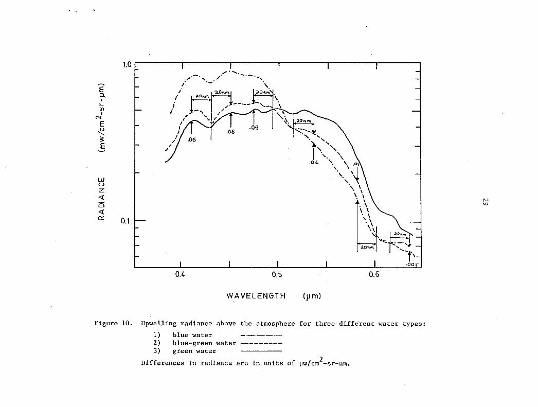
path radiance for a clear sky. Wilson and Austin (1978) have measured

path radiance at two wavelengths for a wide variety of atmospheric

conditions. These data are reproduced in Figure 11. From these plotted

values it appears that, on the clearest day, the radiance at 661 nm was

about 0.6 ~w/cm2-sr-nm and the path radiance at 459 nm was about 2.8

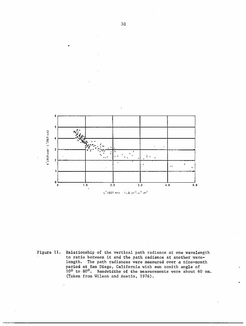
2 ~w/cm -sr-nm. The solid triangles in Figure 12 represent these minimum

radiances. These values represent an absolute lower limit to the upwelling

radiance measured by a satellite sensor. Another estimate of this

E ::l.. I ~

III I

N

E ~ ~ E

w u z « o <t: ~

1.0 'f-~~:::.c=----'-----'------'---",'

, ..... ,/' ...... -

• .J- "

0.1

, I

i

I

I

0.4

:10"", '. -:lO"",

-iI

\" , . '\~Or\'" 'Il.

-- .... '. .. ", " ...

0.5

WAVELENGTH

'. " '. , , \.0

.0(, \ \ {

(~m)

. \ '. '. \ '. \

\ \ . \ '. , \.\ . \

\ \ . \ \,

0.6

...... -f\ .OO~

Figure 10. Upwelling radiance above the atmosphere for three different water types:

1) blue water _._.-._.-2) blue-green water ---------3) green water

Differences in radiance are in units of llw/cm2-sr-nm.

N \.0

30

5

:: c

;; 4 to .--l

3

-CT>

'" .,. 2

~-:+ +~/~ .. \~

'+ +~ + + t* ,..... ." ·r +_., .... . . . ,,-.4 _ .. :: ... . '. , , . ,

+, . . , i ,.' . , . . , , ,

'-l . , " ,

o o 1.0 2.0 3.0 4.0 5.0

Figure 11. Relationship of the vertical path radiance at one wavelength to ratio between it and the path radiance at another wave­length. The path radiances were measured over a nine-month period at San Diego, California with sun zenith angle of 10° to 80°. Bandwidths of the measurements were about 60 nm. (Taken from Wilson and Austin, 1976).

-E ::l... I ~

VI I

N

E u

~ .E

<1.1 U c: c::s "0 c::s

0;:

10.0

1.0

0.1 0.4

.............. A ...........

= o

----....

0.5

...... ....... ,

....... ,

0.6

31

iii o

~ ... ... . ..... ...........

0.7

WAVELENGTH

II

o

...... , ...... ..........

0.8

(J..Im)

............

......................... ...... ......

0.9

.......

o

......... o

Figure 12. Estimates of the range of spectral radiances measured above the atmosphere for a variety of atmospheric conditions and water types.

A minimum path radiance (Wilson and Austin, 1978) A path radiance measurements (Wilson and Austin, 1978) o minimum radiance measurements from Landsat data

over ocean waters. • maximum clear water radiance for high haze conditions

from Landsat data. o maximum turbid water measurements from Landsat data • • expected maximum radiance.

1.0

32

minimum radiance ~vas provided by Hezernak ~ al., (1976) >vho calculated

the upHelling radiance above the .:.-tmosphere ~vhen the solar zenith angle

was 45° and the visibility was 23 km with a haze H (Diermendjian, 1969).

Haze H is used to describe a marine or coastal haze. The calculated

results are shown in Figure 12 as the lower solid line. This line is

somewhat higher than the measured values probably because of the assumption

of higher haze conditions than existed during the measurements. A pair

of path radiance measurements for higher haze conditions fit the predicted

curve quite well (open triangles, 6. , on Figure 12).

The set of measurements in Figure 11 suggest that there is a relation­

ship between the path radiance at one wavelength and that at another.

Wilson and Austin (1978) state that this relationship has been verified.

We will use this fact to draw a line through the low radiance points

which is roughly parallel to the calculations by Wezernak ~ al., (1976).

This then will be the lower end of the sensitivity range needed for

water observations.

As a further check on these values, Landsat data for clear waters

on the continental shelf off of Delaware was reviewed. The open circles,

() , represent the lowest values observed in any of the available data.

It is interesting to note that the circles agree well with the calculations

by Wezernak et al., (1976). The value at 950 nm represents the lowest

possible count value for the Landsat 2 MSS in band 7, i.e. this is the

dark current. Landsat 2 is incapable of lower measurements.

In order to estimate the upper limit of radiance needed we first

estimated the maximum radiance over clear water for high haze conditions.

The solid circles, 41, are the radiance values from Landsat data over

clear shelf water for data which· was marginally useful because of haze

33

and cloud conditions. Again, measured values for path radiance (Wilson

and Austin, 1978) in this range is plotted (open circles, ()) and all

the points have been connected with a line. The next step was to estimate

the maximum range of radiance values which might be expected for water

targets. To do this, the Landsat data was again searched, this time for

the maximum radiances for water areas. The search was not limited to

particular haze conditions. The open squares, [J, represent the highest

values found. The radiances in the visible are from extremely turbid

water in the Delaware River; the IR radiances were found in shelf waters

at the sight of a suspected oil slick. The high radiance values were

found on different scenes than the low radiance values. Nonetheless,

the difference between the high and low values were taken as the maximum

range to be expected for a single scene, and this difference was used to

plot the maximum radiance range expected in each band for very hazy

days. These points are plotted using solid squares, Cl. The upper

limit for the sensitivity range was chosen to be half again higher in

radiance than the maximum estimates in order to allow for the possibility

of extremely bright targets that might appear. The maximum sensitivity

is represented by the upper solid line. The total dynamic range needed

for coastal water observations is then given by the lower dotted line

and the top solid line in Figure 12.

The final question to be asked here is: "Given the dynamic range

just presented, what is required in order to have the required radiometric

sensitivity?" The controlling factor here is the precision of the data.

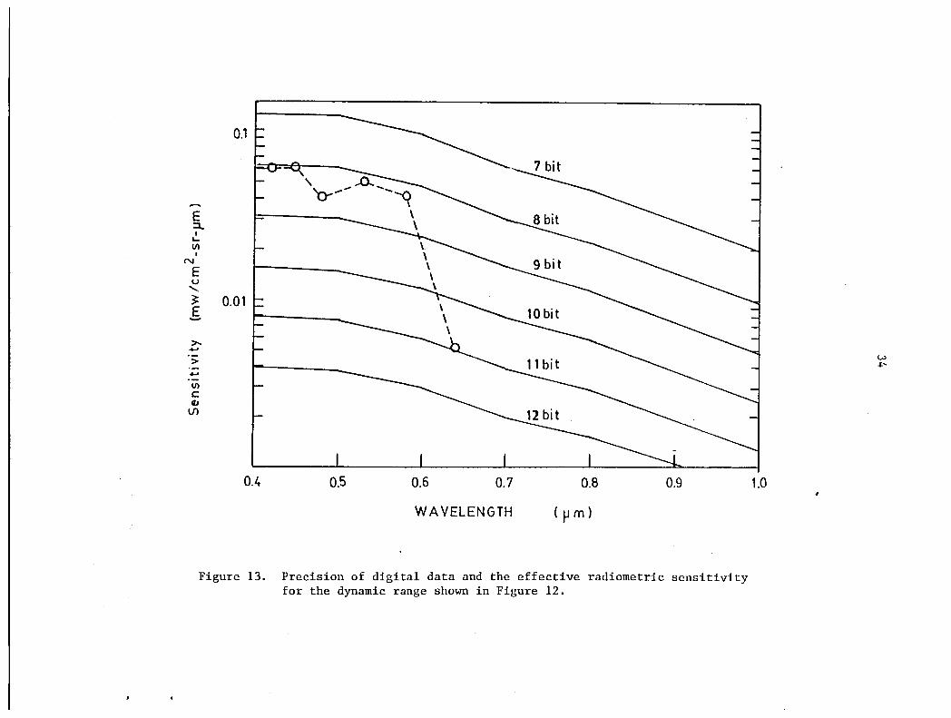
Figure 13 shows the estimated radiometric sensitivity needed to detect

subtle variations in ocean color spectra. Assuming the dynamic range

given above and a linear gain, the precision required is 8-bit data for

E ::J... I ~

III I

N

E u

........

0.1

~ 0.01 oS ,...r---_ >-..... > ..... III C IIJ

Ul

0.4 0.5 0.6 0.7

WAVELENGTH

0.8

( pm)

0.9

Figure 13. Precision of digital data and the effective radiometric sensitivity for the dynamic range shown in Figure 12.

1.0

w ~

35

the 400-600 nm region and 11- or l2-bit data for ~.;ravelengths greater

than 600 nm. Certainly, 8-bit data is necessary and attainable.

Spatial resolution, swath width and coverage freguency

There is often a tendency among researchers, the prese~t authors

included, to wish for higher and higher resolution. It seems as if

there is always some feature which is almost but not quite detectable

and that higher resolution might bring it within the range of detection.

This wish tends to wane when the researcher is faced with the very real

problems usually associated with higher resolution digital data. Data

processing, storage and manipulation become increasingly difficult and

time consuming projects. For research purposes the increase in complexity

may be acceptable for marginal improvements in results, but for opera­

tional systems higher spatial (or spectral) resolution than is necessary

for the task at hand can only increase delays in processing and raise

the cost of the final product. Wherever possible the resolution should

be appropriate for the task.

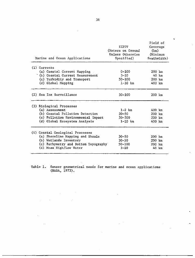
Surprisingly little information is available on resolution require­

ments for any remote sensing application. Most of the stated requirements

for spatial resolution seem to be estimates based more on intuition than

on experimental evidence. One such set of estimates (NASA, 1973) is

presented in Table 1. These values seem quite reasonable and there is

little reason to alter these estimates. Some comments are in order,

however. One of the principal advantages of remote sensing in general

is the ability to cover relatively large areas effectively instantaneously.

Monitoring projects which cover limited regions often require higher

resolution and high frequency coverage than has been available from

satellite systems. Such projects are often better suited to aircraft

36

Marine and Ocean Applications

(1) Currents (a) Coastal Current Happing (b) Coastal Current Heasurement (c) Turbidity and Transport (d) Global Mapping

(2) Sea Ice Surveillance

(3) Biological Processes (a) Assessment (b) Coastal Pollution Detection (c) Pollution Environmental Impact (d) Global Ecosystem Analysis

(4) Coastal Geological Processes (a) Shoreline Mapping and Shoals (b) Wetlands Inventory (c) Bathymetry and Bottom Topography (d) Hean High/Low Water

EIFOV (Meters on Ground Unless Otherwise

Specified)

0-100 3-10

50-100 1-10 km

30-100

1-2 km 30-50 30-300 1-10 km

30-50 30-50 50-100

3-10

Field of Coverage

(km) (Minimum

Swathwidth)

200 km 40 km

200 km 400 km

200 km

400 km 200 km 200 km 400 km

200 km 200 km 200 km

40 km

Table 1. Sensor geometrical needs for marine and ocean applications (NASA, 1973).

37

remote sensing. Examples-might include observations of tidal ~arshes

and creek~, surveillance of pollution along rivers, monitoring and/or

mapping of thermal plumes and detailed surveillance of oil spills. For

these projects a 1m to 10m resolution would be preferable.

Satellite systems are particularly well-suited to observations of

large areas where extremely high resolution is not required. For most

coastal water surveillance, 50-100m resolution is quite adequate. Near

to shore and within bays and estuarines a 30-S0m resolution may be

required due to the presence of point sources of pollution and generally

smaller scales of motion. Farther offshore and into the deep ocean the

scales of motion become quite large and the importance of small pollution

events decrease. The resolution requirements may then diminish to hun­

dreds of meters. In such cases it is worthwhile to trade off the

spatial resolution for better spectral resolution, improved radiometric

sensitivity, larger field of coverage and a higher coverage frequency.

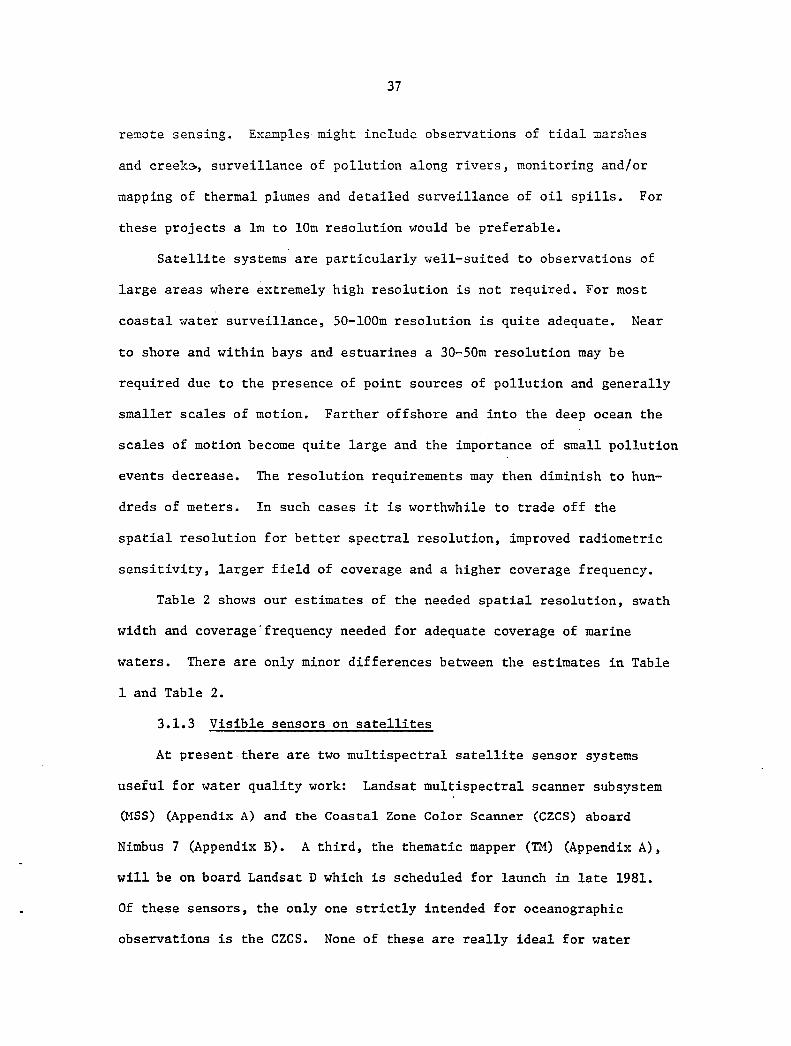
Table 2 shows our estimates of the needed spatial resolution, swath

width and coverage'frequency needed for adequate coverage of marine

waters. There are only minor differences between the estimates in Table

1 and Table 2.

3.1.3 Visible sensors on satellites

At present there are two multispectral satellite sensor systems

useful for water quality work: Landsat multispectral scanner subsystem

(MSS) (Appendix A) and the Coastal Zone Color Scanner (CZCS) aboard

Nimbus 7 (Appendix B). A third, the thematic mapper (TM) (Appendix A),

will be on board Landsat D which is scheduled for launch in late 1981.

Of these sensors, the only one strictly intended for oceanographic

observations is the CZCS. None of these are really ideal for water

38

Regime IFOV S~vath ~vidth Freguency

Shelf waters

Chlorophyll Sludge Iron-acid waste Oil 200m SOOkm daily Current pattern Oceanic fronts

Internal waves 30-S0m 200km monthly

Near shore (bays & estuarines)

Turbidity } Major current pattern 30-S0m 200km weekly Wetland inventory

Pollution detection 30-S0m IOOkm daily Frontal systems } Shoreline mapping IO-20m IOOkm bi-weekly Shoals

Table 2. Suggested spatial and temporal coverage for satellite observations of coastal waters.

39

quality monitoring. The Landsat NSS has adequate resolution (80m) for

most monitoring tasks but the coverage frequency is too low and the ~

, radiometric sensitivity is inappropriate. The latter can be seen

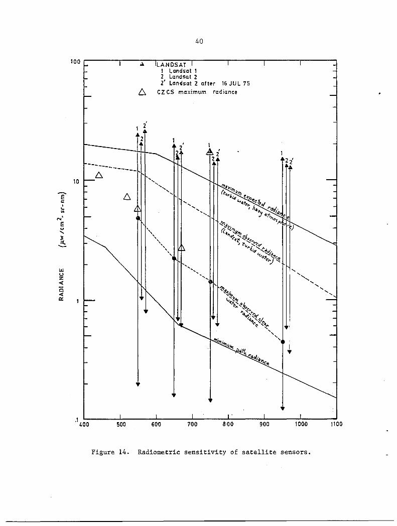
explicitly in Figure 14. The maximum and minimum radiance expected from

a ~vater target for extreme conditions are represented by the t~vo solid

lines ~vhich have been taken from Figure ·12. The sensitivity range for

the Landsat bands (vertical lines, solid arrowheads) easily exceeds the

maximum expected radiance in all bands and is essentially insensitive to

the lower ranges of radiance in bands 6 and 7.

The CZCS, although the bandwidths and choice of wavelengths is gen-

erally superior to that of the MSS, has poorer resolution (800m, nadir)

which is adequate only for offshore work, and will often preclude

identification of a pollutant by spatial features (dumping pattern).

The gain settings on the CZCS are set for water observations, but this,

too, may pose a problem. The maximum radiance (saturation) for the

lowest gain setting of the CZCS is shoWn on Figure 14 with open triangles.

These saturation values are well below the maximum radiances observed

for turbid waters in Landsat data and, in fact, below the maximum radiance

of a fresh iron-acid waste plume as observed by Landsat on a clear day

(25 Aug. 75). It would appear that the CZCS is really designed for

observation of relatively clear waters, and that spectral detail would

be lost due to saturation when observing very turbid waters. Thus, the

CZCS may be an excellent instrument for observations of the relatively

clear continental shelf and shelf slope waters, but may not be very

useful for nearshore observations.

The Thematic Mapper (TM) will provide improvements in both spatial

and spectral resolution over theMSS system. The TM, however, will be

-E c I

"-11\

N'

E u ..... ~

..==.

UJ U Z < Ci < 0:::

40

100 ~------~--~--'--------r------~-------'--------r-----~

-------

10

.1 400 500

after 16JUL75

L:. CZ CS maximum radiance

i 1

2

, " , , , , ,

600

, , , ,

, , , " ... ,

900

Figure 14. Radiometric sensitivity of satellite sensors.

1100

41

subject to the same radiometric and temporal li~itations as the }fSS.

Nonetheless, the TIl is expected to provide a signifi~ant improvement

over the MSS for nearshore and estuarine observations.

Several other sensors are either in the proposal or planning stages.

Two which may be important for ocean color observations are the Multispectral

Resource Sampler (MRS) (Appendix C) and the updated CZCS in the National

Oceanic Satellite System (NOSS) (Appendix D) program. The }ffiS will mark

a slight improvement in sensitivity over the }lSS and TM and allow a wide

variety of narrow band, filter combinations which could prove quite

advantageous. Perhaps the major advantage of the MRS, though, is the

pointing capability. The MRS is designed to be pointed in flight at

chosen targets. Even though the MRS will be flown on a satellite which

is likely to have orbital characteristics similar to Landsat, the pointing

capability can increase coverage frequency to ~ to ~ days. This could

be extremely useful for monitoring pollutant dispersion and transport.

The NOSS program includes an updated version of the CZCS. This

CZCS will probably provide better spectral resolution by adding several

bands and a slightly improved spatial resolution due to a lower orbit.

However, the most important aspect of the NOSS program for water quality

monitoring is that it includes plans for near real-time data products

(NASA/DOC/DOD, 1979). This aspect of satellite remote sensing has not

received a great deal of attention, yet the rapid availability of data

is extremely important for many monitoring tasks.

3.2 Thermal infrared region

Infrared radiation at wavelengths from 3 to 14 pm is called the

thermal IR region. There are two atmospheric windows within this region

42

(3-5 1J!!l and 8-14 1J!!l). For !!lost purposes the 8 1J!!l to 14 1J!!l ,vave1ength

band is preferred to the other atmospheric ,vindmv since 8-14 '.lm band

includes the maximum intensity of the radiant energy flux for the earth's

surface. Thermal IR radiation is absorbed by the glass lenses of con-

ventional optical systems and cannot be detected by photographic films.

Special detectors and optical-mechanical scanners are used to detect and

record images in the thermal IR region.

Thermal IR images record the radiant heat of a material. The

radiant heat is a measure of the ability of the material to absorb and

radiate thermal energy. Thermal scanners record the radiant temperature

of the water surface which, with proper calibration and surface truth,

can be related to absolute temperatures in waters free of surface con-

tamination. A major advantage of thermal imagery is that it is not

dependent on daylight. It is, however, severely limited by weather and

the interpretation of the data may vary depending on whether the data

was collected during the day or at night. La Violette (1975) describes

the difficulties:

"When clouds are present between the sensor and the ocean, the sensor records cloud rather than ocean radiation temperatures. The surface thermal features of the ocean in these cases are effectively blocked from the satellite's view. Thin clouds and water vapor affect sensor data by making the ocean's surface appear cooler than it actually is. The amount of apparent cooling is directly proportional to the amount of water vapor in the air.

"Another problem in the utilization of satellite infrared sensors for oceanographic purposes, is the type of energy being measured. The "sea surface temperature" collected by infrared sensors is the equivalent blackbody radiation of the first milli­meter of the surface layer ••• Sufficient radiation loss occurs at night, so that the surface radiation temperature in the early morning hours can easily

43

represent a dynamic m~:nng to a depth of several meters. Duing the daytime, however, isolation offsets the radiation loss by a variable amount. If there is no mechanical mixing, such as ,,,hen \Vind speeds are less than 10 knots, then infrared daytime measurements may be the radiation of a surface film quite different in temperature than the water a fe,,, centimeters deeper."

Thermal IR data has been used for observations of oceanic and shelf

water circulation patterns using the temporal variations of the ocean's

temperature field (Hal1iwa11, 1978; Bisagni, 1976), and for observations

of coastal upwelling (Szekie1da, 1973). As higher resolution systems

become available, smaller details of the circulation patterns and thermal

effluents will come within range of observation. Accurate absolute

temperature maps are not yet possible since they require complex ca1ibra-

tions to account for atmospheric effects. Absolute accuracy is presently

limited to about 2°C. Relative changes of about 0.5°C are detectable.

3.3 Microwave region

Micro\Vave systems have the greatest potential for observation of

ocean dynamics. A considerable amount of research has been done exploring

the many applications of microwave remote sensing for oceanographic

purposes. Unfortunately, very little satellite data is available at

present and very little is likely to be available in the near future.

Waters ~ al. (1975) and the CORSPERS (1977) report revie,,, the develop-

ment of satellite microwave measurements. The only sensor presently

available is the SMMR aboard Nimbus 7, and the only other data which

will be available during the 1980-1985 time frame will be from systems

flown on the space shuttle (SIR-A, SIR-B, SIMS, SMMRE). The NOSS program,

should it be approved, will contain several microwave sensors and would

be available 1985 or later. We will consider microwave systems, although

44

only briefly, because of the likelihood of their eventual importance in

monitoring systems.

Microwave systems are unique in that both active and passive systems

are feasible for satellite applications. Active (radar) and passive

(radiometer) systems have very different characteristics and applications.

An excellent review of the characteristics of these systems can be found

in the CORSPERS (1977) report. The description below is largely excerpted

from this report.

The microwave radiometer measures the electromagnetic energy radiated

towards it from some target or area. Being a passive sensor, it is

related more to the classical optical and IR sensors than to radar,

its companion active microwave sensor. The energy detected by a radiometer

at microwave frequencies is the thermal emission from the target itself

as well as thermal emission from the sky that arrives at the radiometer

after reflection from the target. The thermal emission depends on the

product of the target's absolute temperature and its emissivity. At

microwave frequencies, it is the change in emissivity rather than the

change in temperature that produces most of the significant differences

between the various targets. The intervening atmosphere between the

target and the radiometer can have an adverse effect on the measurement

by attenuating the desired energy due to its own temperature and emissivity.

One of the major limitations of a spaceborne radiometer is its

relatively crude resolution, which is a consequence of the antenna

beamwidth and the long range to the target area. The thermal radiation

from the body of temperature T is not as great in the microwave as in

the IR region. The microwave radiometer is also less sensitive. There

are, however, significant differences in the brightness temperature

45

measurement at microwave frequencies that make the radiometer of interest

as a remote sensor. Measurements at microwave frequencies, both active

and passive, are less affected by haze, fog, and clouds than are those

of IR and optical sensors. In fact, at lower frequencies microwave

radiation is particularly insensitive to the presence of clouds, fog and

haze. Since the sensitivity to water is frequency dependent, a multi­

frequency system can provide measurements of atmospheric water vapor and

liquid water over the oceans, thus providing sufficient information to

calibrate surface temperature measurements.

Other measurements possible with the microwave radiometer are the

temperature profile, sea-ice boundaries, discrimination of first-year

and multi-year ice, salinity of water, oil slicks and sea state.

An active microwave sensor (radar) is responsive to the reflected

energy from sharp discontinuities in the transmission medium or from

those features of the target that have sizes comparable to the sensor's

wavelength. Thus, the energy of a microwave radar signal interacts with

those features of a target that have characteristic sizes on the order.

of centimeters, while optical and IR sensors are sensitive to scatterer

sizes on the order of micrometers. The radar senses different characteristics

of a target than an optical or an IR sensor. A radar image should

therefore not be expected to look like or contain the identical information

as an optical image even if the resolutions are comparable.

Large ocean waves (gravity waves) behave like an ensemble of specular

reflectors so that the strength of the scattered radiation is proportional

to the slope of the gravity waves. However, ocean waves comparable to

the wavelengths of the microwave systems used show resonant, or Bragg,

scattering effects for angles of incidence larger than 20°. This type

46

of scattering is controlled by the capillary waves, which in turn depend

on the local short-term surface wind field and the ocean water surface

tension. The latter changes when an oil film covers the water surface,

resulting in a modification of the character of the capillary waves.

Thus, oil is detectable with active microwave systems.

There are three different instruments which will be useful for

remote sensing of ocean waters: altimeters, scatterometers and imagery

radars. The radar altimeter can provide information on sea-surface

topographic features: sea surface height, and significant wave height.

The scatterometer, viewing the oceans at 0° to 10° incidence angles,

provides sea-state information through the detection of the slope statistics

of the ocean waves. For higher incidence angles, local wind fields can

be determined.

Perhaps the most versatile instrument is the imaging radar. This

instrument can provide a variety of information on wave patterns and

dynamic behavior. Imaging radar can function through clouds to provide

information on wave heights, wave patterns near shore, oil spills, and

current patterns.

A rather thorough discussion of the physics of radar interactions

with the ocean and the uses and limitations of radar systems in remote

sensing is provided in the Active Microwave Workshop Report (NASA,

1975).

The Scanning Multichannel Microwave Radiometer (SMMR), which is

aboard the Nimbus 7 satellite, will provide data on sea surface temperature

and near-surface winds on a nearly all-weather basis. The surface wind

speed, a parameter which is not available from other remote systems will

be particularly valuable for transport and dispersion predictions. The

47

S}~m is a five-wavelength; dual polarized scanning radiometer. The

multiple wavelengths are needed to correct the observed brightness tem­

perature for atmospheric absorption and emission.

IV. The Role of Satellite Remote Sensing in Environmental Monitoring

4.1 Specific targets

4.1.1 Photosynthetic pigments

The remote detection of chlorophyll and other photosynthetic

pigments has been an important research topic for several years. The

major emphasis has·been on using the relationship of chlorophyll to

phytoplankton to assess primary productivity of ocean waters. While

primary productivity is not the goal of a pollution monitoring system, a

knowledge of the productivity of the waters in the vicinity of a dump or

spill can be important to the assessment of the impact of a pollution

event. More directly, an unusual plankton bloom or an unusual drop in

chlorophyll levels can be an indicator of a pollution event.

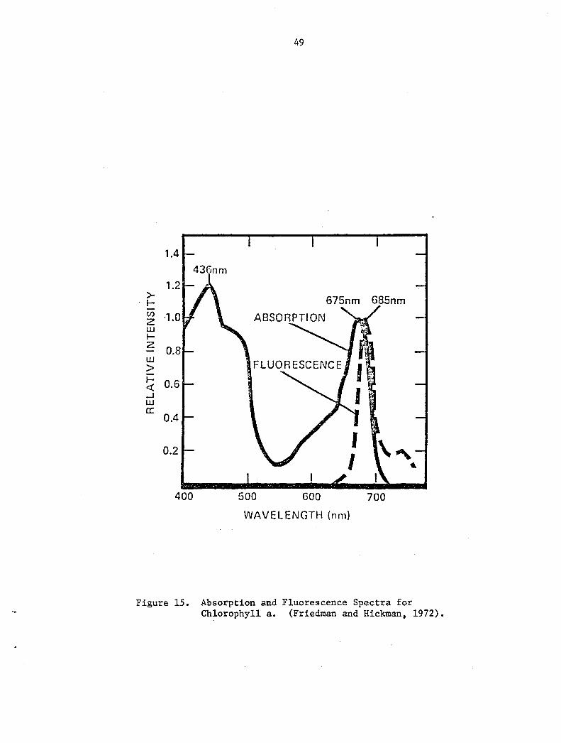
The uniqueness of a pigment's signature rests more in the absorptive

and fluorescence characteristics of the pigment than in the scattering

characteristics. Chlorophyll absorbs most strongly in the blue and has

a second absorption peak around 670-680 nm with the absorption minimum

occurring around 550 nm (Figure 15). Carotenoids are more effective in

absorbing light in the region around 500 nm. When carotenoids are

present the absorption minimum will generally shift towards the red.

Several investigators have attempted to use these absorption charac­

teristics to detect chlorophyll. Clarke et a1. (1970) used a ratio of

the upwelling radiance at 540 nm to that at 460 nm. This ratio was

later also used by Curran (1972) and by Arvesen ~ a1. (1971). This

48

two band ratio has worked rather vlell in several instances, but has

proven troublesome in applying ~vhen the chlorophyll is masked by the

presence of suspended particulates, absorbing materials such as yellow

substance or pigments other than chlorophyll.

Smith and Baker (1978) suggested an algorithm using measured reflec­

tance at three wavelengths to disentangle the chlorophyll signal. Wilson

~ ale (1978) applied this algorithm (using the wavelengths 471 nm, 547

nm and 662 nm with a 22 nm bandwidth) to data collected in the N.Y.

Bight. While the corel1ation with the chlorophyll measurements was

quite good it was found that the algorithm had to be adjusted for the

ambient water mass. Three classes were found: class 1 for near coastal

waters, class 2 for offshore waters and class 3 for waters in the vicinity

of an acid dump.

Duntley et al. (1972) pointed out that, for a given species of

phytoplankton in an otherwise homogeneous water mass, changes in the

phytoplankton concentration will not alter the reflectance of optically

deep water at a particular v7avelength. This "hinge point" will occur at

different wavelengths for different species but appeared between 500-540

nm for the species which Duntley et al. (1972) modeled. Presumably, a

band in this wavelength region would be useful for observing changes in

the background water.

Recently it has become apparent that the presence of chlorophyll

can be detected by passive remote sensing of the fluorescence maximum

around 685 nm. Neville and Gower (1977) and Morel and Prieur (1977)

have reported such observations and Gordon (1979) corroborated this by

establishing that the quantum efficiencies of the chlorophyll fluorescence

are sufficient to produce the observed effect. Thus, it would seem that a

>­l-t/)

2 w I-2

1.4

1.2

w > l-e:( 0.6 -1 w 0::

0.4

0.2

400

49

436nm

675nm G85nm

ABSORPTION

500 GOO 700

WAVELENGTH (nm)

Figure 15. Absorption and Fluorescence Spectra for Chlorophyll a. (Friedman and Hickman, 1972).

50

band in the vicinity of 685 nrn should aid in detecting chlorophyll.

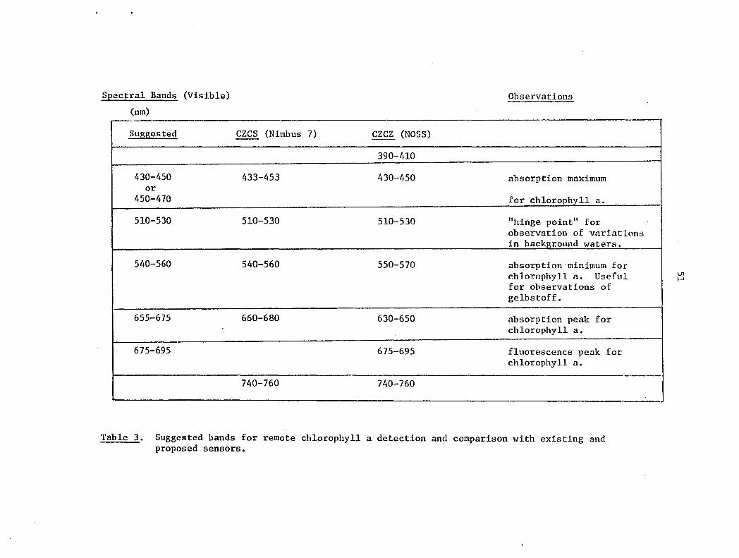
Given the above considerations, we would suggest a 5-band sensor

for the detection of chlorophyll. The spectral bands and their purposes

are given in Table 3. The bands suggested in Table 3 are essentially

the same as those of the CZCS except that the CZCS red band (660-680 nm)

overlaps the two bands suggested here. If fluorescence is important,

such a band would give a higher reading than might be expected. It may

be somewhat premature to suggest a chlorophyll fluorescence band since

passive fluorescence observations are few and none have been made from

satellite altitudes. However, the observations, although few,are rather

convincing and suggest that a fluorescence band would be valuable. The

expanded CZCS being proposed for the NOSS program includes such a band.

As far as spectral characteristics are concerned the CZCS is far

preferrable to any existing or approved satellite system for the detec­

tion of chlorophyll in oceanic waters. Yet there are limitations to the

applicability of the CZCS. Because of the relatively crude spatial res­

olution (800 m) only large features will be seen. Features smaller than

a few kilometers will not be discernable and larger areas which are dynam­

ically complex on a small scale may appear washed out. This suggests that

the CZCS would be most appropriate for continental shelf and open ocean.

This predilection for offshore waters is further supported by the radio­

metric sensitivity of the CZCS. As can be seen in Figure 14, the CZCS

channels (open triangles, A ) will, probably be driven off scale when

observing very turbid water or even clear waters on very hazy days even

at the lowest gain settings. The CZCS should provide excellent data for

the relatively clear offshore waters but will be of limited use in turbid,

nearshore or estuarine waters.

Spectral Bands (Visible)

(nm)

Suggested

430-450 or

450-470

510-530

540-560

655-675

675-695

CZCS (Nimbus 7)

433-453

510-530

540-560

660-680

740-760

Observations

CZCZ (NOSS)

390-410

430-450 absorption maximum

for chlorophyll a.

510-530 "hinge point" for observation of variations in background waters.

550-570 absorption minimum for chlorophyll a. Useful for observations of ge1bstoff.

630-650 absorption peak for chlorophyll a.

675-695 fluorescence peak for chlorophyll a.

740-760

Table 3. Suggested bands for remote chlorophyll a detection and comparison with existing and proposed sensors.

I

I !

VI t-'

52

Other satellite systems may be useful to some extent, especially

~ .... hen smaller features are of interest. The Landsat HSS spectral bands

are clearly not designed for observations of marine chlorophyll. I'mile

it may be possible to use Landsat data for chlorophyll observations it

will be a limited role, probably restricted to observations of offshore

waters where phytoplankton can dominate as the optically important

material in the water. One important use would be to use the MSS data to

provide detailed spatial information in conjunction with the spectral

observations of the CZCS. If the CZCS data shows an area to be high in

chlorophyll, Landsat data may be able to show some of the smaller scale

distribution patterns of the chlorophyll.

The 1M will be an improvement over the HSS both in the spectral

bands available and in the radiometric sensitivity. The spectral bands

are still rather wide and do not really correspond to the ideal for

chlorophyll sensing, but they are some~"hat better placed than the HSS

bands. Some further improvement will be possible ~vith the HRS. Again,

the bands have not been chosen with marine chlorophyll sensing in mind,

but with the selectable filters it should be possible to have a reasonable

set of spectral bands. Given the proposed bands the best selection for

chlorophyll detection would probably be as follows:

Array 1, Filter 2 (540-560 nm): This corresponds exactly to one of

recommended bands.

Array 2, Filter 2 (670-690 nm): This band should be useful for the

fluorescence measurement. It is

slightly shifted toward the blue

into the chlorophyll absorption

peak.

53

Array 3, Filter 3 (630-690): Subtracting the radiance measured by

the red band above (670-690 nm) ~.;rill

give a value for the radiance in the

region 630-670. This is some,.;rhat

broader than desirable but it does

correspond to the chlorophyll absorb­

tion peak.

Array 4, Filter 3 (400-420) or Filter 4 (490-510):

4.1.2 Iron-acid waste

It is difficult to say which of these

filters is preferable; they bracket

the chlorophyll absorption maximum.

Iron-acid waste, a by-product of titanium dioxide production, is

one of the pollutants most visible from space. Several investigators

have reported on the detection of this waste from satellite, notably

Bowker and Witte (1977), Schmidt (1978) and Philpot and Klemas (1979).

The optically important component of the iron-acid waste is a ferric­

hydroxide precipitate which forms when the acid waste is buffered by the

seawater. Lewis (1977) presents remotely measured spectra of the iron­

acid waste (Figure 16). The spectra show a peak in the observed radiance

at about 580 nm for high concentrations of acid. The peak shifts towards

the blue for very low concentrations finally approaching the ambient

water signature with a peak at about 480 nm. Little response was seen

at any concentration for the spectral region from 425-470 nm and at a

narrow band around 740 nm. Lewis (1977) suggested using the ratio of

observed radiance at 580 nm to that at 440 nm as a measure of the acid

concentration.

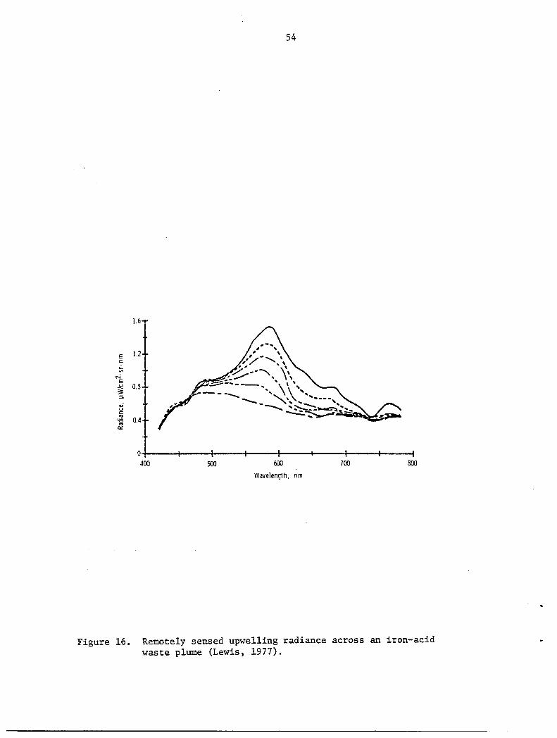
54

1.6

E 1.2 c: .:.. '" N E ~ 0.3 ;;: :::l.

oi u c: "' 'i5 0.4 "' a::

0 400 500 600 700 800

Waveleng1h. nm

Figure 16. Remotely sensed upwelling radiance across an iron-acid waste plume (Lewis, 1977).

55

Further examination of the upwelling radiance curves presented by

Lewis (1977) reveal that the change in radiance across an iron-acid

plume does not occur at the same rate at all wavelengths. The family of

curves presented in Figure 16 shows an initial rapid increase in radiance

around 500 nm and then a leveling off. In contrast, at 650-700 nm the

initial change is rather slow but later becomes quite rapid. It is not

possible to say why these sorts of variations occur, although Philpot

and K1emas (1979) have suggested that they may be due to changes in

concentration with depth. Spectral bands in these regions might assist

in the detection and quantification of iron-acid waste. Thus, preferred

bands for observation of ironacid waste are as follows (in order of

preference):

Band 1: 570-590 nm

Band 2: 450-470 nm

Band 3: 500-520 nm

Band 4: 650-670 nm

-maximum response to the presence of the

iron-acid waste.

-minimum response to the presence of

iron-acid waste.

-indicator of the shift of the peak towards

the blue, - possibly related to depth

distribution.

-radiance changes in this region are at a

different rate than either Band 1 or Band 3.

The Landsat MSS bands have been used quite successfully in identifying

the acid waste although some difficulty has been encountered in distin­

guishing between acid waste and other materials (Philpot and K1emas,

1979). The difficulty is probably due to the very broad bands of the

MSS.

The TM bands are a significant improvement over the MSS bands for

56

detection and identification of acid. Using the TIl bands it should be

possible to distinguish the acid from other materials. The ~ms can

improve on this somewhat by substituting a filter in the 490-510 nm

range (Array 4, filter 4). Spectrally the CZCS bands are preferable to

any of the above sensors. However, the CZCS has poor spatial resolution

'''hich will degrade the sensitivity of the sensor for iron-acid waste

detection.

4.1.3 Sewage Sludge

Ocean dumping of sewage sludge has occurred for years and is likely

to continue for several years to come unless acceptable alternatives are

found. There have been relatively few remote observations of sludge

dumps partially due to the rapid settling rate of the particulate fraction

of the sludge (Kupferman and Murphy, 1973). Johnson et ale (1977) have

reported on an experiment designed to remotely detect se,,,age sludge.

Observations included a fresh, very highly concentrated IIspotll dump as

well as a fresh IIlinell dump. The "linell dump is the typical dumping

pattern. Spectra of these dumps, normalized to ocean water spectra, are

shown in Figure 17 (from Johnson et al., 1977). The normalized spectra

of the fresh "spot" dump actually peaks in the near infrared and is

quite strong in the red. The peak radiance is quite broad. The normalized

spectra from the line dump also has a broad peak in the red/infrared.

In both cases the spectral peaks shift toward the blue with age. These

spectra suggest that it is primarily the particulate pahse which is

responsible for the appearance of the sludge. The absolute change in

radiance is strong in all bands (Figure 18) indicating that the upwelling

spectral radiance is due to IIwhite", or wavelength independent scattering.

Since there are no apparent absorption or emission lines, a system

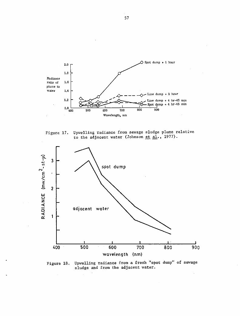
57

2.0 Spot dump + 1 hO!lr

1.8

Radiance ratio of 1.6 plume to water 1.4

1.2

1.0 400 500 600 700 L_J;~~~~:::::L=_:-:~~:::::-:~~~r~/=.:L~in~e:.5dump + 4 hr-45 min Spot dump + 4 hr-45 min

900

Wavelength, nm

Figure 17. Upwelling radiance from sewage sludge plume relative to the adjacent water (Johnson ~ al., 1977).

~ , -1/1 I

N

E u ...... ~ .§.

w u z « c « a::

3 spot dump

2

adj acent water

400 500 600 700 800 900 wavelength (nm)

Figure 18. Upwelling radiance from a fresh "spot dump" of sewage sludge and from the adjacent water.

58

designed for detection of se~age sludge might best have 3 or 4 rather

broad spectral bands ranging from about 450 nm to 800 or 900 nm. The

first four TH bands are probably near ideal for detection of sludge.

Landsat bands should be quite good. In fact the spectral bands available

on any of the existing or planned multispectral systems are good for the

detection of sludge. The difficulty in sludge detection will lie, not

with the spectral characteristics, but with spatial resolution and

radiometric sensitivity. Like the acid waste and most other regulated

ocean-dumped materials, the sludge actually covers an area of less than

25 km2

even when the dumpsites are considerably larger. The resolution

of the CZCS (800m) is such that only about 50-70 pixels will cover areas

with any sludge in it, and most of those pixels will view water predominantly;

a line dump is often less than a kilometer wide. As can be seen from

Figure 17, the spectral signature of the sludge from aircraft data in

which the pixels are entirely within the boundaries of the plume, rapidly

approach the background water signature. Such a low background signature

would be effectively lost if averaged with the background water signature.

The Landsat resolution is far better for observation of "line" dumps;

unfortunately, the Landsat radiometric sensitivity is not. The TM is

the best compromise available. The TM has both improved spatial resolution

and radiometric sensitivity over the Landsat HSS.

4.2 General monitoring

In Section II of this report several broad criteria were described

which will define the role of satellite systems in the monitoring of

coastal water properties. Using these criteria several categories of

environmental monitoring were discussed. We ~vill nO,"l review these

categories in reference to the use of satellite remote sensing in the 1980's.

59

1) Fast response operations: Satellite systems will not generally be

appropriate for this type of monitoring during the 1980's. The coverage

frequency of satellite systems, especially those with higher resolution

is rather poor. For instance, the coverage frequency for the Landsat MSS

(80 m resolution) is 18 days. As the spatial resolution is degraded the

swath width of the sensor can be increased. The CZCS, with 800 m resolution,

will provide once daily coverage in the visible region. One answer to the

problem of coverage frequency is built into the design of the proposed

Multispectral Resource Sampler (MRS). This sensor may be pointed in both

the along track and cross track directions allowing frequent observations

of a particular target area at high resolution (15 m).

Another factor that is crucial to fast-response operations is real-

time or near real-time availability of data. With the exception of thermal

imagery and the accompanying visible, single-band imagery, no satellite

data is presently available in anything approaching real-time. Landsat

digital data is generally available to the general user in two to three

months after the overpass. The lag time for CZCS data is about to 9-10

months although this should improve as the data processing procedures are

finalized. The large lag times are not so much a fault in the system

designs (both Landsat and the CZCS were experimental in nature and geared

toward research rather than operational uses) as they are a problem in using

the system for monitoring purposes. Rapid data availability is very

important for monitoring purposes and efforts should be made to reduce the

time delay in receiving data. Such efforts might include cost/benefit

analyses of timely satellite data for a monitoring program and perhaps a

pilot program to explore the problems involved in providing usable data

rapidly. A program of this type is being proposed as part of the NOSS program.

60

As mentioned above, the one exception to the rule is thermal imagery

from the NOAA satellites. The Dvice-daily imagery is routinely available

several days after an overpass and can be made available on the same day.

However, thermal imagery is something of a special case, i.e., it is single­

band data which requires minimal processing and little or no enhancement

to be put into a usable form. The multispectral data which could be used

for environmental monitoring may require far more processing before it is

in a usable form. For instance, producing chlorophyll distribution maps

from CZCS data requires that the data first be corrected to remove

atmospheric effects before the chlorophyll algorithms can be applied.

2) Long-term monitoring: Satellite systems are particularly well­

suited to observations of large regions and for repetitive coverage over

long time periods. Thus satellite observations could be extremely valuable

to monitoring programs for which the goal is observation of long term

changes in environmental parameters. The utility of a particular sensor

for a specific monitoring task will depend heavily on the sensor charac­

teristics and the orbital characteristics of the parent satellite.

3) Enforcement monitoring: One of the advantages of satellite

remote senSing is that data is collected routinely and periodically. For

enforcement purposes this means that, if a pollution event or its effects

are detectable from satellite, data will be available before, after and

perhaps even during the pollution event.

4) Historical data acquisition: Again, since satellite data is

collected routinely and periodically, it can provide an excellent source

for observation of long-term changes.

61

V. Conclusions

1) The satellit2s ~vhich ~vill be available during the 1980 I s ~vill

not be ideal for water quality assessment or pollution

monitoring in the near coastal waters ,-.There pollution and environ­

mental changes may have the most obvious impact. These are

areas in which small scale changes can be quite important.

Unfortunately, systems having the best spatial resolution (HSS,

TM, MRS) have poor spectral characteristics and the systems

with the best spectral characteristics for water color observa­

tions (CZCS) have poor spatial resolution. Nonetheless, the

systems having sufficient spatial resolution will provide

valuable information for environmental monitoring particularly

in the role of spatial extrapolation of surface measurements.

2) The CZCS is uniquely appropriate to the observation of ~vater

color. Although the spectral response was designed specifically

for chlorophyll detection, the spectral bands should be adequate

for many other uses. The CZCS will be primarily useful in

offshore waters both because its relatively poor resolution

(800 m) will not show adequate detail of very near-shore or

estuarine phenomena and because the radiometric sensitivity is

carefully tuned to the low radiance of offshore waters.

3) Satellite remote sensing should be an important part of most

moderate or large scale monitoring programs. In most cases,

if the spatial and temporal requirements of the program are

compatible with the satellite data characteristics, the

satellite data will be a valuable addition to the program:

62

a) The satellite imagery provides a synoptic vi~v of large

areas impossible to achieve by other means. Using this

data a conventional data base ~~y be greatly expanded and

extrapolated spatially.

b) Satellite data can be used to provide a historical perspec­

tive on the environment. Even without simultaneous surface

truth, satellite imagery can be used to develop a qualitative

assessment of circulation patterns, shoreline changes,

sediment distribution and surface temperature variations.

4) Much research remains to be done before satellite remote sensing

data can be used to obtain quantitative results operationally.

A solid groundwork has been laid by research in the use of

Landsat MSS data and aircraft systems for water observations

and in theoretical studies of the radiative transfer properties

of the ocean and atmosphere. Research efforts in the early

1980's to demonstrate operational use of satellite data for

quantitative observations could lead to operational systems in

the mid to late 1980's. This is most likely to be the case with

the CZCS scanner as applied to offshore monitoring of chlorophyll,

and with the continually improving thermal data which will be

available during the early 1980's.

5) More attention should be given to cost/benefit analysis of

using satellite data especially in long-term operational

monitoring efforts. A particular test project would have to be

defined such as monitoring chlorophyll distributions using the

CZCS and minimal surface truth compared to purely ship-based

observations. \~i1e there is every reason to expect that the

63

remote observations would be cost effective, this has not been

demonstrated by any careful study.

6) Efforts should be made to improve the time lag between a satellite

overpass and the availability of the data. The proposed NOSS

project (NOSS, 1979) includes real time data processing as a

major part of the project. Such efforts should be undertaken

since long lag times are a major drawback to the use of satellite

data for operational monitoring.

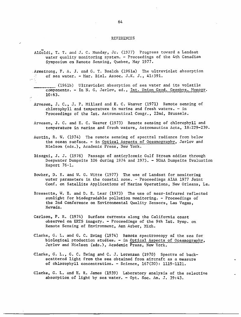
64

REFERENCES

" A1fo1di, T. T. and J. C. Munday, Jr. (1977) Progress toward a Landsat water quality monitoring system. - Proceedings of the 4th Canadian Symposium on Remote Sensing, Quebec, May 1977.

Armstrong, F. A. J. and G. T. Boalch (1961a) The ultraviolet absorption of sea water. - Mar. BioI. Assoc. J.K. J., 41:591.

(1961b) Ultraviolet absorption of sea ~vater and its volatile components. - In N. G. Jerlov, ed., Int. Union Geod. Geophys. Monogr. 10:63.

Arvesen, J. C., J. P. Millard and E. C. ~veaver (1971) Remote sensing of chlorophyll and temperature in marine and fresh waters. - in Proceedings of the Int. Astronautical Congr., 22nd, Brussels.

Arvesen, J. C. and E. C. Weaver (1973) Remote sensing of chlorophyll and temperature in marine and fresh waters, Astronautica Acta, 18:229-239.

Austin, R. W. (1974) The remote sensing of spectral radiance fro~ below the ocean surface. - in Optical Aspects of Oceanography, Jerlov and Nielson (eds.), Academic Press, Ne~v York.

Bisagni, J. J. (1976) Passage of anticylconic Gulf Stream eddies through Deepwater Dumpsite 106 during 1974 and 1975. - NOAA Dumpsite Evaluation Report 76-1.

Bowker, D. E. and W. G. Witte (1977) The use of Landsat for monitoring water parameters in the coastal zone. - Proceedings AlAA 1977 Joint Conf. on Satellite Applications of Marine Operations, New Orleans, La.

Bressette, W. E. and D. E. Lear (1973) The use of near-infrared reflected sunlight for biodegradable pollution monitoring. - Proceedings of the 2nd Conference on Environmental Quality Sensors, Las Vegas, Nevada.

Carlson, P. R. (1974) Surface currents along the California coast observed on ERTS imagery. - Proceedings of the 9th Int. Symp. on Remote Sensing of Environment, Ann Arbor, Mich.

Clarke, G. L. and G. C. Ewing (1974) Remote spectroscopy of the sea for biological production studies. - in Optical Aspects of Oceanography, Jerlov and Nielsen (eds.), Academic Press, New York.

Clarke, G. L., G. C. Ewing and C. J. Lorenzen (1970) Spectra of back­scattered light from the sea obtained from aircraft as a measure of chlorophyll concentration. - Science, 167(20): 1119-1121.

Clarke, G. L. and H. R. James (1939) Laboratory analysis of the selective absorption of iight by sea water. - Opt. Soc. Am. J. 39:43.

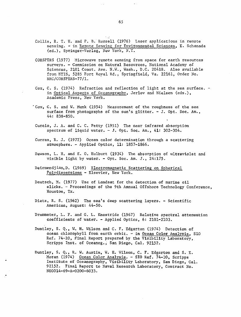
65

Collis, R. T. H. and P. B. Russell (1976) Laser applications in remote sensing. - in Remote Sensing for Environmental Sciences, E. Schanada (ed.), Springer-Verlag, New York, N.Y.

CORSPERS (1977) Microwave remote sensing from space for earth resources surveys. - Commission on Natural Resources, National Academy of Sciences, 2101 Const. Ave. N.W., Wash., D.C. 20418. Also available from NTIS, 5285 Port Royal Rd., Springfield, Va. 22161, Order No. NRC/CORSPERS-77/l.

Cox, C. S. (1974) Refraction and reflection of light at the sea surface. -in Optical Aspects of Oceanography, Jer10v and Nielsen (eds.), Academic Press, Ne,. York.

'Cox, C. S. and W. Munk (1954) Measurement of the roughness of the sea surface from photographs of the sun's glitter. - J. Opt. Soc. Am., 44: 838-850.

Curcio, J. A. and C. C. Petty (1951) The near infrared absorption spectrum of liquid water. - J. Opt. Soc. Am., 41: 302-304.

Curran, R. J. (1972) Ocean color determination through a scattering atmosphere. - Applied Optics, 11: 1857-1866.

Dawson, L. H. and E. O. Hulburt (1934) The absorption of ultraviolet and visible light by water. - Opt. Soc. Am. J., 24:175.

Deirmendjian,D. (1969) Electromagnetic Scattering on Spherical Po1ydispersions - Elsevier, New York.

Deutsch, M. (1977) Use of Landsat for the detection of marine oil slicks. - Proceedings of the 9th Annual Offshore Technology Conference, Houston, Tx.

Dietz, R. s. (1962) The sea's deep scattering layers. - Scientific American, August: 44-50.

Drummeter, L. F. and G. L. Knestride (1967) Relative spectral attenuation coefficients of water. - Applied Optics, 6: 2101-2103.

Duntley, S. Q., w. H. Wilson and C. F. Edgarton (1974) Detection of ocean chlorophyll from earth orbit. - in Ocean Color Analysis, SIO Ref. 74-10, Final Report prepared by the Visibility Laboratory, Scripps Inst. of Oceanog., San Diego, Cal. 92152.

Duntley, S. Q., R. W. Austin, W. H. ~Vilson, C. F. Edgarton and S. E. Moran (1974) Ocean Color Analysis. - SIO Ref. 74-10, Scripps Institute of Oceanography, Visibility Laboratory, San Diego, Cal. 92152. Final Report to Naval Research Laboratory, Contract No. N00014-69-A-0200-6033.

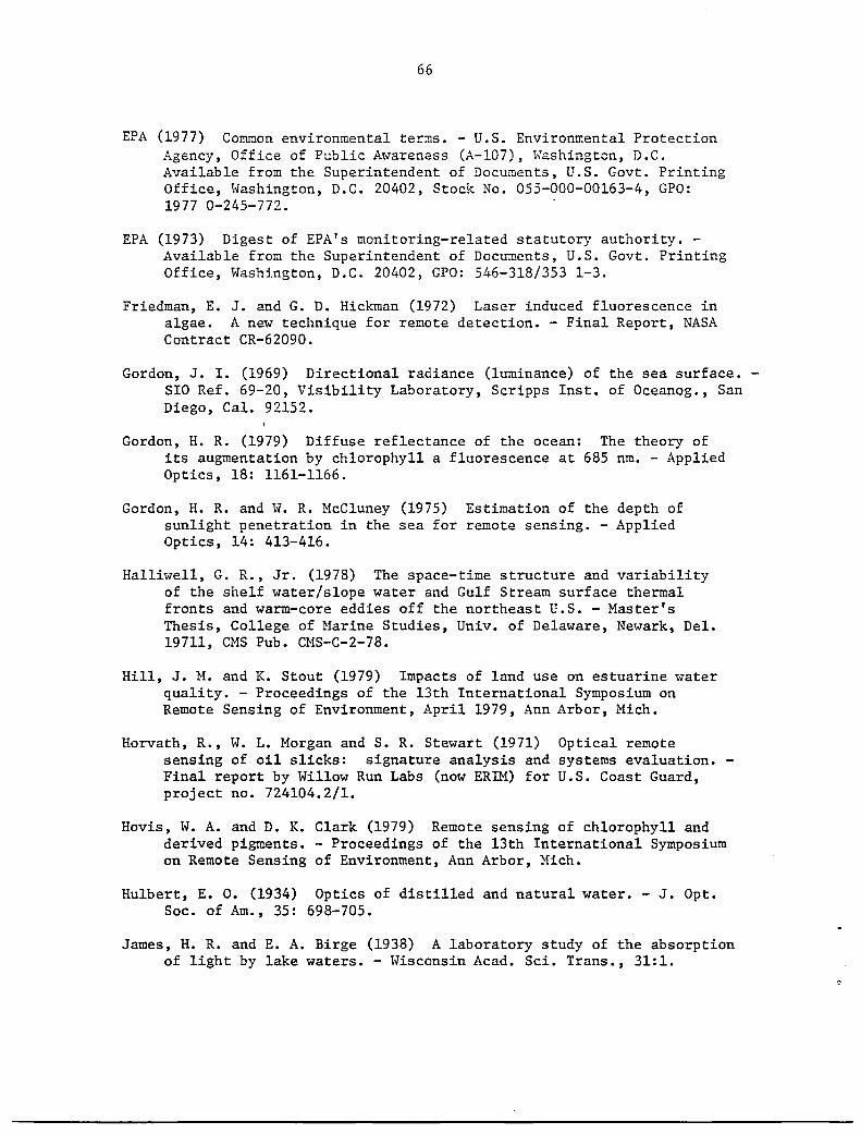
66

EPA (1977) Common environmental terms. - U.S. Environmental Protection Agency, Office of Public A~V'areness (A-107), \{ashingtcn, D.C. Available from the Superintendent of Documents, U.S. Govt. Printing Office, Washington, D.C. 20402, Stock No. 055-000-00163-4, GPO: 1977 0-245-772.

EPA (1973) Digest of EPA's monitoring-related statutory authority. -Available from the Superintendent of Documents, U.S. Govt. Printing Office, Washi.ngton, D.C. 20402, GPO: 546-318/353 1-3.

Friedman, E. J. and G. D. Hickman (1972) Laser induced fluorescence in algae. A new technique for remote detection. - Final Report, NASA Contract CR-62090.

Gordon, J. I. (1969) Directional radiance (luminance) of the sea surface. -SIO Ref. 69-20, Visibility Laboratory, Scripps Inst. of Oceanog., San Diego, Cal. 92152.

Gordon, H. R. (1979) Diffuse reflectance of the ocean: The theory of its augmentation by chlorophyll a fluorescence at 685 nm. - Applied Optics, 18: 1161-1166.

Gordon, H. R. and W. R. McCluney (1975) Estimation of the depth of sunlight penetration in the sea for remote sensing. - Applied Optics, 14: 413-416.

Halliwell, G. R., Jr. (1978) The space-time structure and variability of the shelf water/slope water and Gulf Stream surface thermal fronts and warm-core eddies off the northeast U.S. - Master's Thesis, College of Marine Studies, Univ. of Delaware, Ne~V'ark, Del. 19711, CMS Pub. CMS-C-2-78.

Hill, J. M. and K. Stout (1979) Impacts of land use on estuarine water quality. - Proceedings of the 13th International Symposium on Remote Sensing of Environment, April 1979, Ann Arbor, Mich.

Horvath, R., W. L. Morgan and S. R. Stewart (1971) sensing of oil slicks: signature analysis and Final report by Willow Run Labs (now ERIM) for project no. 724104.2/1.

Optical remote systems evaluation. -U.S. Coast Guard,

Hovis, W. A. and D. K. Clark (1979) Remote sensing of chlorophyll and derived pigments. - Proceedings of the 13th International Symposium on Remote Sensing of Environment, Ann Arbor, Mich.

Hulbert, E. o. (1934) Optics of distilled and natural water. - J. Opt. Soc. of Am., 35: 698-705.

James, H. R. and E. A. Birge (1938) A laboratory study of the absorption of light by lake waters. - Wisconsin Acad. Sci. Trans., 31:1.

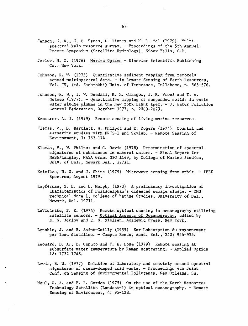
67

Jensen, J. R., J. E. Estes, L. Tinney and H. R. ~fel (1979) Multi­spectral kelp resource survey. - Proceedings of the 5th Annual Pecora Symposium (Satellite Hydrology), Sioux Falls, S.D.

Jerlov, N. G. (1976) Marine Optics - Elsevier Scientific Publishing Co., New York.

Johnson, R. w. (1975) Quantitative sediment mapping from remotely sensed multispectral data. - in Remote Sensing of Earth Resources, Vol. IV, (ed. Shahrokhi) Univ. of Tennessee, Tullahoma, p. 565-576.

Johnson, R. W., I. W. Duedall, R. M. Glasgow, J. R. Proni and T. A. Nelsen (1977). - Quantitative mapping of suspended solids in waste water sludge plumes in the New York Bight apex. - J. Water Pollution Control Federation, October 1977, p. 2063-2073.

Kemmerer, A. J. (1979) Remote sensing of living marine resources.

Klemas, V., D. Bartlett, W. Philpot and R. Rogers (1974) Coastal and estuarine studies with ERTS-l and Skylab. - Remote Sensing of Environment, 3: 153-174.

Klemas, V., W. Philpot and G. Davis (1978) Determination of spectral signatures of substances in natural waters. - Final Report for NASA/Langley, NASA Grant NSG 1149, by College of Marine Studies, Univ. of Del., Newark Del., 19711.

Kritikos, R. N. and J. Shiue (1979) Microwave sensing from orbit. - IEEE Spectrum, August 1979.

Kupferman, S. L. and L. Murphy (1973) A preliminary investigation of characteristics of Philadelphia's digested sewage sludge. - CMS Technical Note 1, College of Marine Studies, University of Del., Newark, Del. 19711.

LaViolette, P. E. (1974) Remote optical sensing in oceanography utilizing satellite sensors. - Optical Aspects of Oceanography, edited by N. G. Jerlov and E. S. Nielsen, Academic Press, New York.

Lenoble, J. and B. Saint~Guilly (1955) Sur Labsorption du rayonnement par leau distillee. - Compte Rendu, Acad. Sci., 240: 954-955.

Leonard, D. A., B. Caputo and F. E. Roge (1979) Remote sensing at subsurface water temperature by Raman scattering. - Applied Optics 18: 1732-1745.

Lewis, B. w. (1977) Relation of laboratory and remotely sensed spectral signatures of ocean-dumped acid waste. - Proceedings 4th Joint Conf. on Sensing of Environmental Pollutants, New Orleans, La.

Maul, G. A. and R. R. Gordon (1975) On the use of the Earth Resources Technology Satellite (Landsat-I) in optical oceanography. - Remote Sensing of Environment, 4: 95-128.

68

Horel, A. (1974) Optical properties of pure ~'later and pure sea ~vater. in Optical Aspects of Oceanographv, edited by Jerlov and Nielsen, Academic Press, New York.

Morel, A. and L. Prieur (1977) Analysis of variations in ocean color. -Limnology and Oceanography, 22:709

Mueller, J. L. (1976) Ocean color spectra measured off the Oregon coast: characteristic vectors. - Applied Optics, 15: 394-402.

Mueller, J. L. (1979) The remote measurement of ocean color. - in Remote Sensing for Ocean Dynamics, College of Marine Studies Technical Report (in preparation).

Mumola, P. B. (1973) Multiwavelength lidar for remote sensing of chlorophyll ~ in phytoplankton. - Proceedings Second Environmental Quality Sensor Conf., Las Vegas, Nevada.

NASA (1975) Active microwave remote sensing of oceans. - in Active Microwave Horkshop Report edited by R. E. Matthews, NASA SP-376 U.S.G.P.O. 033-000-00624-1.

NASA (1973) Advanced scanners and imagery systems for earth observations. NASA Special Publication SP-335, Government Printing Office.

NASA/DOC/DOD (1979) NOSS, National Oceanic Satellite System. - Available from NOSS Program Manager, Goddard Space Flight Center, Greenbelt, Md. 20771.

Neville, R. A. and J. F. R. Gower (1977) Passive remote sensing of phytoplankton via chlorophyll a fluorescence. - J. Geophys. Res., 82: 3487-3493.

Ohlhorst, C. H. and G. S. Bahn (1978) Quantitative mapping of particulate iron in an ocean dump using remotely sensed data. - Proceedings: ACSM-ASP Annual Spring Convention, ~vashington D.C.

Philpot, H. and V. Klemas (1979) Detection of ocean waste in the New York, Bight. - Final Report prepared for NASA, Langley Research Center, Hampton, Va. 23665, NASA grant NSG 1398.

Sawyer, H. R. (1931) The spectral absorption of light by pure water and Bay of Fundy water. - Contrib. Can. BioI. Fish., New Series, 7:74.

Smith, R. C. and K. S. Baker (1978) Remote sensing of chlorophyll. -Proceedings of XXth meeting COSPAR Symposium on the contribution of space observations to global food information systems.

Schmidt, D. (1978) Some more recent methods for the scientific inves­tigation of dumping of wastes in the North Sea Area. - Proceedings 1st Int. Ocean Dumping Symposium, Univ. of Rhode Island.

•

69

Smith, R. C. and J. E. Tyler (1976) Transmission of solar radiation into natural waters. - Photochem. Photobio1. Rev., 1: 117--155.

Strong, A. E. (1978) Chemical whitings and chlorophyll distribution in the Great Lakes as viewed by Landsat. - Remote "Sensing of Environment, 7: 61-72.

Sullivan, S. A. (1963) Experimental study of the absorption in distilled water, artificial sea water, and heavy water in the visible region of the spectrum. - J. Opt. Soc. Am., 53: 962-968.

Szekie1da, K. H. (1973) The validity of ocean surface temperatures monitored from satellites. - J. Cons. Int. Exp10r. Mer. 35(1): 78-86.

Tyler, J. E. and R. C. Smith (1970) Measurements of Spectral Irradiance Underwater. - Gordon and Breach Science Publ., New York.

Waters, J. W., F. T. Barath, E. Y. Chow, A. F. H. Goetz, E. J. Johnston, J. M. Stacey, J. J. Gustincic, D. H. Staelin, J. A. Kong, E. G. Njoku, K. F. Junzi, D. O. Muhleman, and T. T. Wilheit (1975) The shuttle imaging microwave system experiment. - Proceedings of the IEEE National Telecommunications Conference, New Orleans, La.

White, J. and L. R. Breslau (1978) Remote sensing for oil pollution control along coastal waters of the United States. -- Proceedings of the 12th Int. Symp. on Rem. Sense of Environment, Manila, Philippines.

Wezernak, C. T., R. E. Turner and D. R. Lyzenga (1975) Spectral reflectance and radiance characteristics of water pollutants. - Final Report, NASA Contract NAS1-l3589 by ERIM, P.O. Box 618, Ann Arbor, Michigan, 48107.

Wilson, W. H. and R. W. Austin (1978) Remote sensing of ocean color. -in Proceedings of Ocean Optics V, San Diego, Cal., SPIE, Vol. 160.

Wilson, W. H., R. W. Austin and R. C. Smith (1978) Optical Remote Sensing of chlorophyll in ocean waters. - Proceedings 12th Int. Symposium on Remote Sensing of Environment, Manila, Philippines.

Wilson, W. B. and A. Collier (1972) The production of surface-active material by marine phytoplankton cultures. - J. Marine Research, 30: 15-26 •

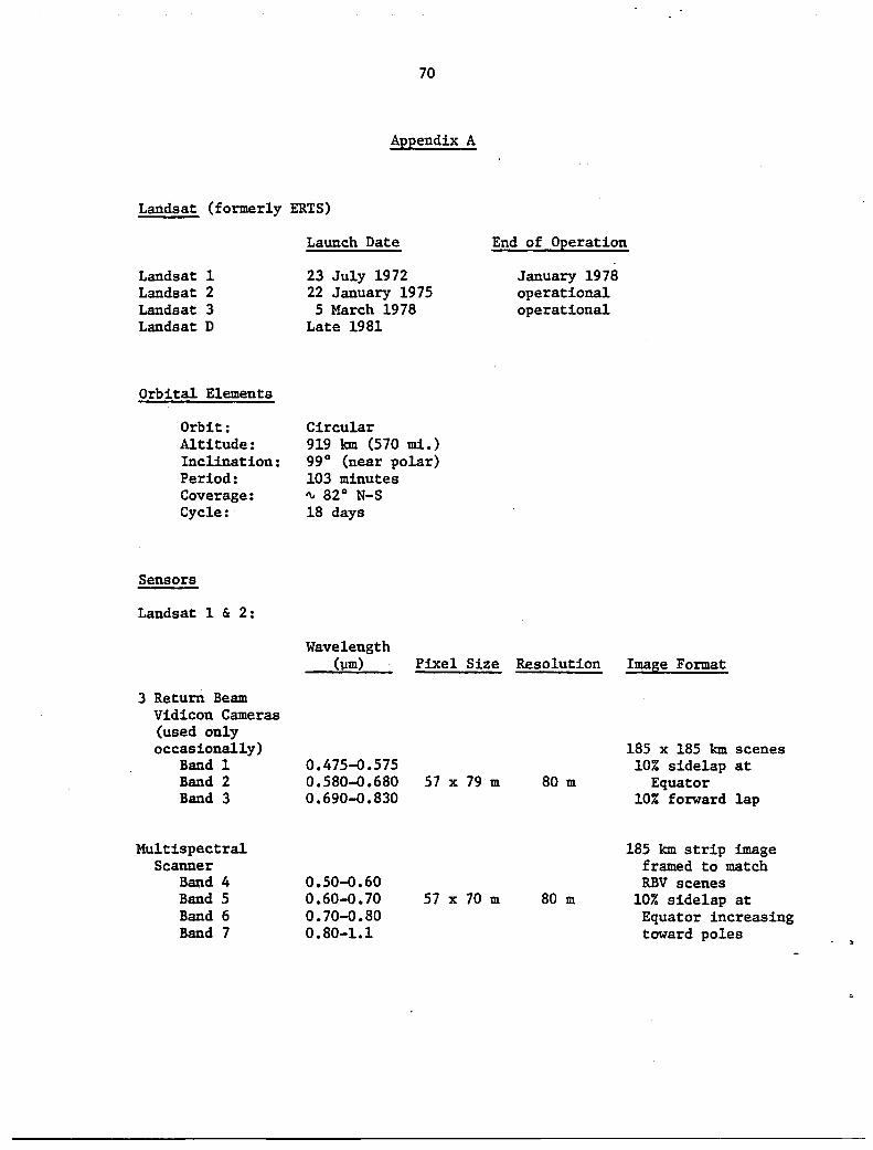
70

Appendix A

Landsat (formerly ERTS)

Landsat 1 Landsat 2 Landsat 3 Landsat D

Orbital Elements

Orbit: Altitude: Inclination: Period: Coverage: Cycle:

Sensors

Landsat 1 & 2:

3 Return Beam Vidicon Cameras (used only occasionally)

Band 1 Band 2 Band 3

Multispectral Scanner

Band 4 Band 5 Band 6 Band 7

Launch Date End of Operation

23 July 1972 22 January 1975 5 March 1978

Late 1981

Circular 919 km (570 mi.) 99° (near polar) 103 minutes '" 82° N-S 18 days

Wavelength

January 1978 operational operational

(~m) Pixel Size Resolution Image Format

0.475-0.575 0.580-0.680 0.690-0.830

0.50-0.60 0.60-0.70 0.70-0.80 0.80-1.1

57 x 79 m

57 x 70 m

80 m

80 m

185 x 185 km scenes 10% sidelap at

Equator 10% forward lap

185 km strip image framed to match RBV scenes

10% sidelap at Equator increasing toward poles

• >

•

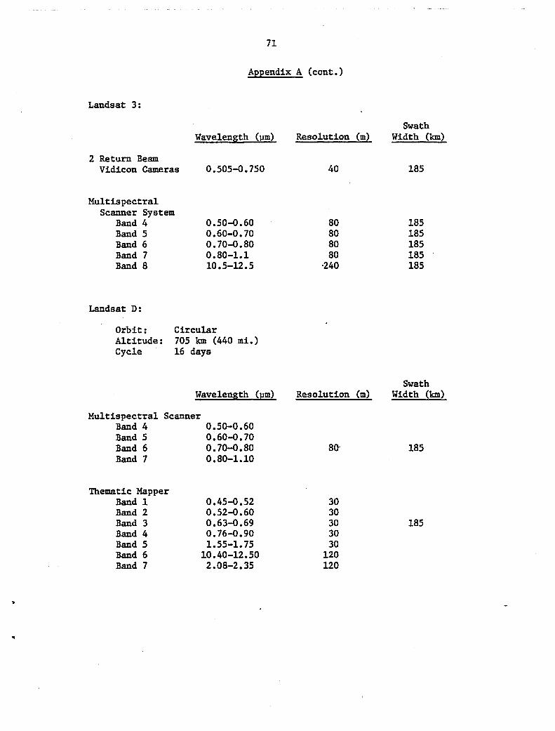
71

Appendix A (cont.)

Landsat 3:

Wavelength (llm)

2 Return Beam Vidicon Cameras 0.505-0.750

Multispectral Scanner System

Band 4 Band 5 Band 6 Band 7 Band 8

Landsat D:

Orbit: Altitude: Cycle

0.50-0.60 0.60-0.70 0.70-0.80 0.80-1.1 10.5-U.5

Circular 705 km (440 mi.) 16 days

Wavelength (llm)

Multispectral Scanner Band 4 0.50-0.60 Band 5 0.60-0.70 Band 6 0.70-0.80 Band 7 0.80-1.10

Thematic Mapper Band 1 0.45-0.52 Band 2 0.52-0.60 Band 3 0.63-0.69 Band 4 0.76-0.90 Band 5 1.55-1.75 Band 6 10.40-12.50 Band 7 2.08-2.35

Resolution (m)

40

80 80 80 80

·240

Resolution (m)

80-

30 30 30 30 30

120 120

Swath Width (km)

185

185 185 185 185 185

Swath Width (km)

185

185

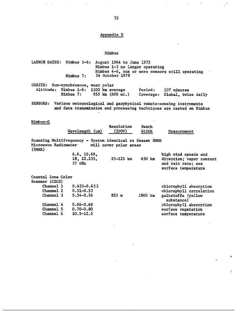
72

Appendix B

Nimbus

LAUNCH DATES: Nimbus 1-6: August 1964 to June 1975 Nimbus 1-3 no longer operating Nimbus 4-6, one or more sensors still operating

Nimbus 7: 24 October 1978

ORBITS: Sun-synchronous, near polar Altitude: Nimbus 1-6: 1100 km average

Nimbus 7: 955 km (600 mi.) Period: 107 minutes Coverage: Global, twice daily

SENSORS: Various meteorological and geophysical remote-sensing instruments and data transmission and processing techniques are tested on Nimbus

Nimbus-G

Wavelength (~m) Resolution

(IFOV) Swath Width --- Measurement

Scanning Multifrequency - System identical to Seasat SMMR Microwave Radiometer will cover polar areas (SMMR)

Coastal Zone Color Scanner (CZCS)

Channel 1 Channel 2 Channel 3

6.6, 10.69, 18, 22.235, 37 GHz

0.433-0.453 0.51-0.53 0.54-0.56

Channel 4 Channel 5 Channel 6

0.66-0.68 0.70-0.80 10.5-12.5

25-125 km

825 m

high wind speeds and 650 km direction; vapor content

and rain rate; sea surface temperature

1800 km

chlorophyll absorption chlorophyll correlation gelbstoffe (yellow

substance) chlorophyll absorption surface vegetation surface temperature

..

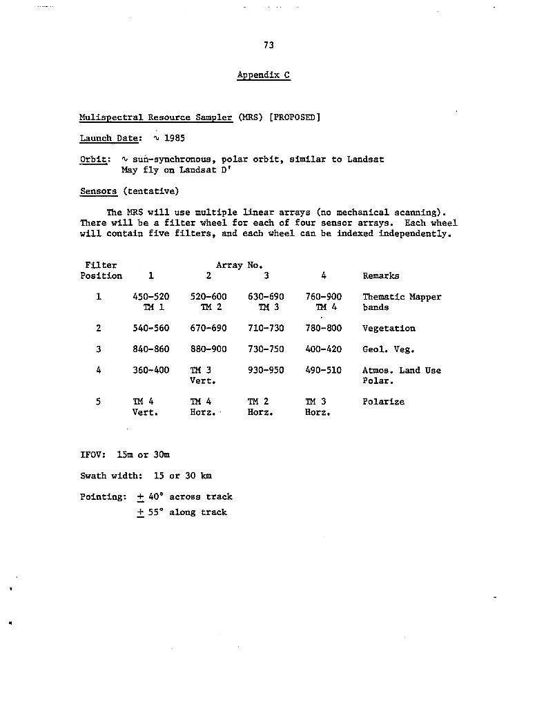
73

Appendix C

Mulispectral Resource Sampler (MRS) [PROPOSED]

Launch Date: ~ 1985

Orbit: ~ sun-synchronous, polar orbit, similar to Landsat May fly on Landsat Dr

Sensors (tentative)

The MRS will use multiple linear arrays (no mechanical scanning). There will be a filter wheel for each of four sensor arrays. Each wheel will contain five filters, and each wheel can be indexed independently.

Filter Array No. Position 1 2

1 450-520 520-600 TMI TM2

2 540-560 670-690

3 840-860 880-900

4 360-400 TM3 Vert.

5 TM4 TM4 Vert. Horz •.

IFOV: 15m or 30m

Swath width: 15 or 30 km

Pointing: + 40° across track

+ 55° along track

3

630-690 TM3

710-730

730-750

930-950

TM2 Horz.

4 Remarks

760-900 Thematic Mapper TM4 bands

780-800 Vegetation

400-420 Geo!. Veg.

490-510 Atmos. Land Use Polar.

TM3 Polarize Horz.

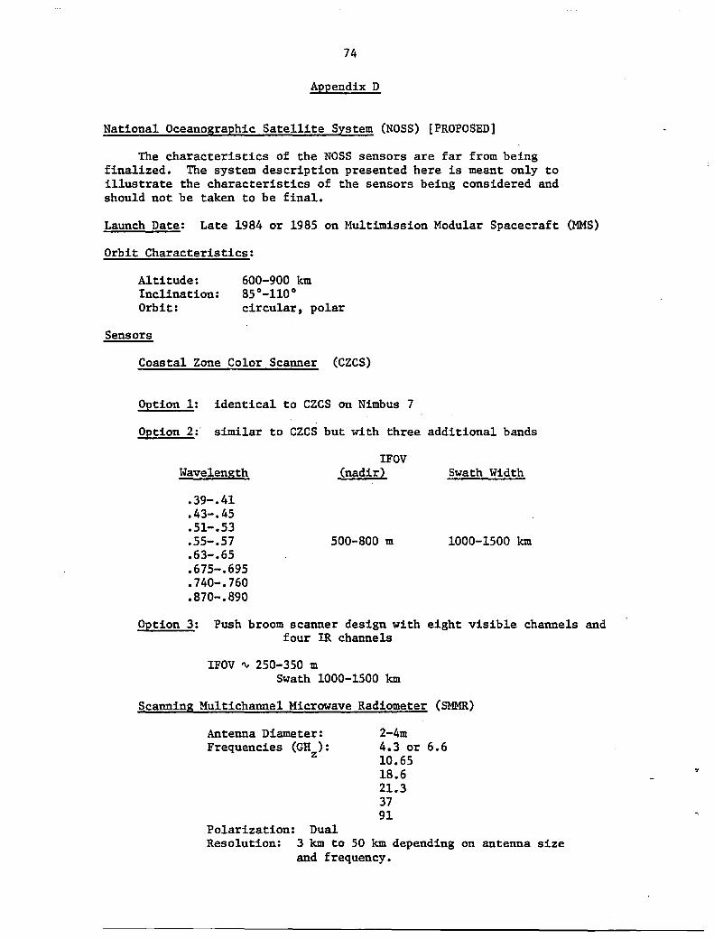
74

Appendix D

National Oceanographic Satellite System (NOSS) [PROPOSED]

The characteristics of the NOSS sensors are far from being finalized. The system description presented here is meant only to illustrate the characteristics of the sensors being considered and should not be taken to be final.

Launch Date: Late 1984 or 1985 on Multimission Modular Spacecraft (MMS)

Orbit Characteristics:

Altitude: Inclination: Orbit:

Sensors

600-900 km 85°-110° circular, polar

Coastal Zone Color Scanner (CZCS)

Option 1: identical to CZCS on Nimbus 7

Option 2:' similar to CZCS but with three additional bands

Wavelength

.39-.41

.43-.45

.51-.53

.55-.57

.63-.65

.675-.695

.740-.760

.870-.S90

IFOV (nadir)

500-S00 m

Swath Width

1000-1500 km

Option 3: Push broom scanner design with eight visible channels and four IR channels

IFOV IV 250-350 m Swath 1000-1500 km

Scanning Multichannel Microwave Radiometer (SMMR)

Antenna Diameter: Frequencies (GH ): z

Polarization: Dual

2-4m 4.3 or 6.6 10.65 lS.6 21.3 37 91

Resolution: 3 km to 50 km depending on antenna size and frequency.

..

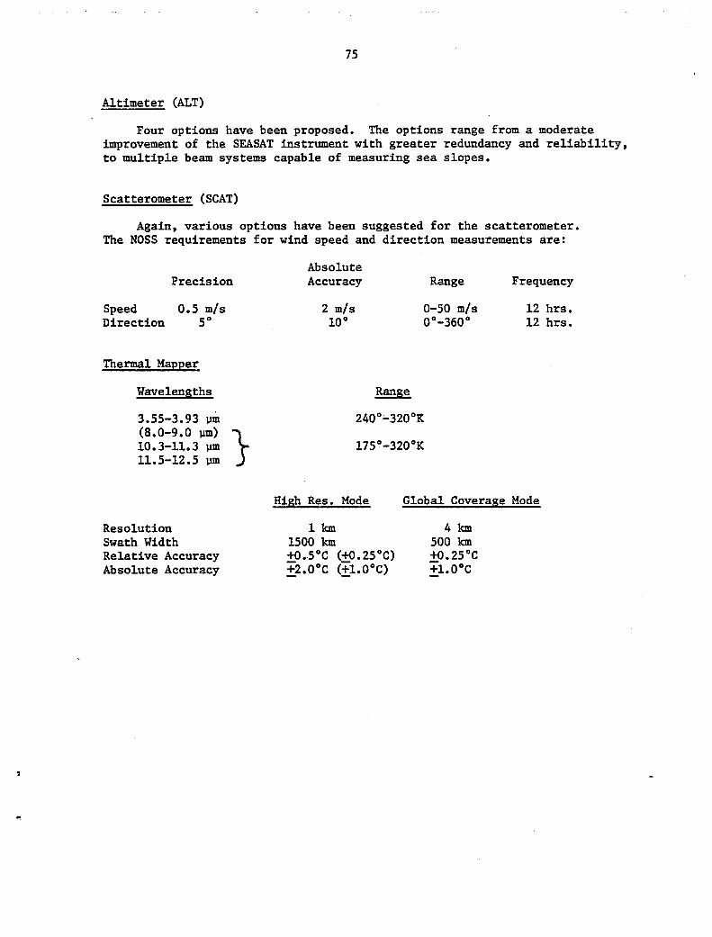
75

Altimeter (ALT)

Four options have been proposed. The options range from a moderate improvement of the SEASAT instrument with greater redundancy and reliability, to multiple beam systems capable of measuring sea slopes.

Scatterometer(SCAT)

Again, various options have been suggested for the scatterometer. The NOSS requirements for wind speed and direction measurements are:

Precision

Speed Direction

0.5 mls 5°

Thermal Mapper

Wavelengths

3.55-3.93 j.lm (8.0-9.0 j.lm) } 10.3-11.3 j.lm 11.5-12.5 j.lm

Resolution Swath Width Relative Accuracy Absolute Accuracy

Absolute Accuracy

2 mls 10°

High Res. Mode

1km 1500 km +O.SoC (+O.2S 0 C) +2.0°C (+1.0 0 C)

Range Frequency

12 hrs. 12 hra.

Global Coverage Mode

4km 500 km +O.2SoC +1.0°C

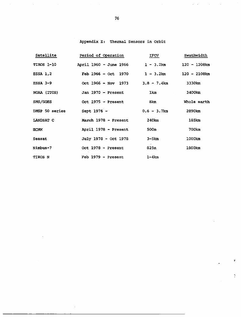
Satellite

TlROS 1-10

ESSA 1,2

ESSA 3-9

NOAA (ITOS)

SMS/GOES

DMSP 50 series

LANDSAT C

HCMM

Seasat

Nimbus-7

TlROS N

76

Appendix E: Thermal Sensors in Orbit

Period of Qperation

April 1960 - June 1966

Feb 1966 - Oct 1970

Oct 1966 - Nov 1973

Jan 1970 - Present

Oct 1975 - Present

Sept 1976 -

March 1978 - Present

April 1978 - Present

July 1978 - Oct 1978

Oct 1978 - Present

Feb 1979 - Present

IFOV

1 - 3.2km

1 - 3.2km

3.8 - 7.4km

lkm

8km

0.6 - 3.7km

240km

500m

3-5km

825m

1-4km

swathwidth

120- 1208km

120 - 2108km

3330km

3400km

Whole earth

2890km

185km

700km

1000km

1800km

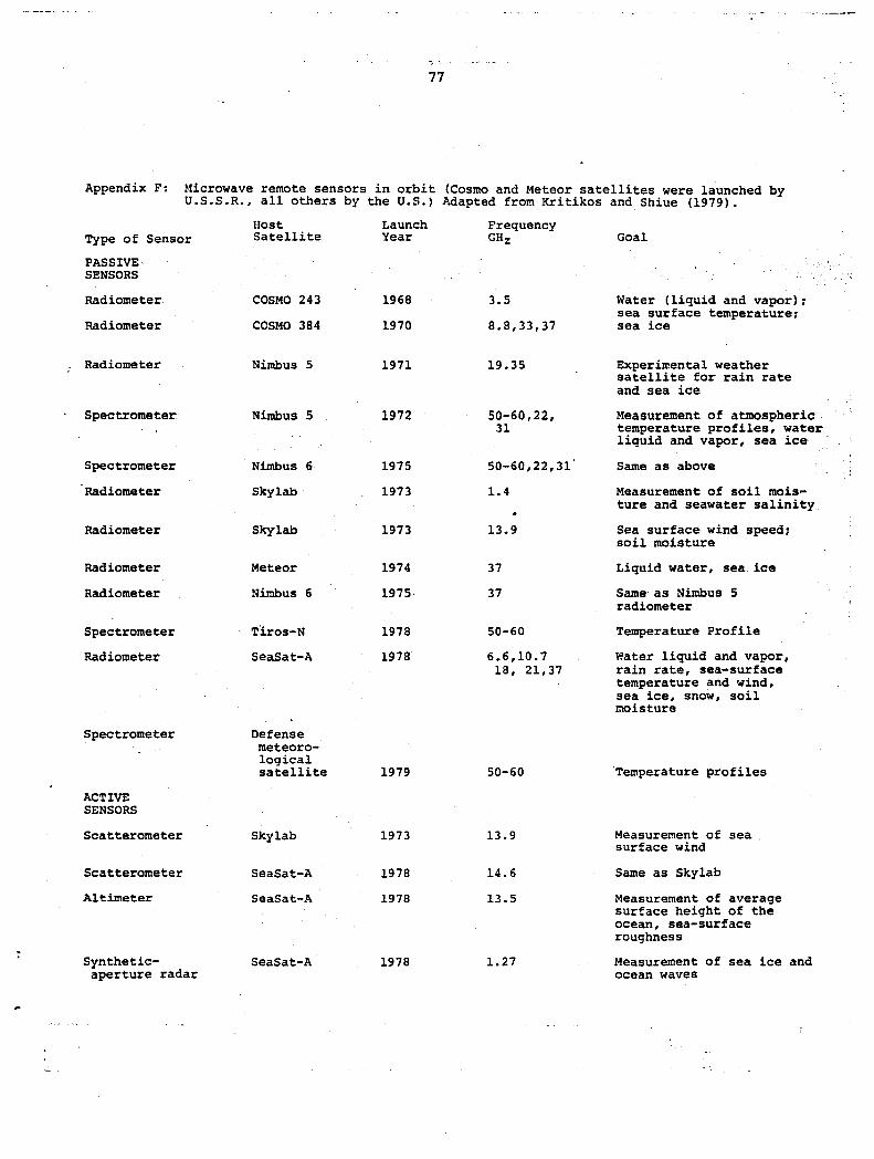
77

Appendix F: Microwave remote sensors in orbit (Cosmo and Meteor satellites were launched by U.S.S.R., all others by the U.S.) Adapted from Kritikos and Shiue (1979).

Type of Sensor

PASSIVE SENSORS

Radiometer

Radiometer

Radiometer

Spectrometer

Spectrometer

Radiometer

Radiometer

Radiometer

Radiometer

Spectrometer

Radiometer

Spectrometer

ACTIVE SENSORS

Scatterometer

Scatterometer

Altimeter

Synthetic­aperture radar

Host Satellite

COSMO 243

COSMO 384

Nimbus 5

Nimbus 5

Nimbus 6

Skylab

Skylab

Meteor

Nimbus 6

Tlros-N

SeaSat-A

Defense meteoro­logical satellite

Sky lab

SeaSat-A

SeaSat-A

SeaSat-A

Launch Year

1968

1970

1971

1972

1975

1973

1973

1974

1975

1978

1978

1979

1973

1978

1978

1978

Frequency GHz

3.5

8.8,33,37

19.35

50-60,22, 31

50-60,22,31

1.4

13.9

37

37

50-60

6.6,10.7 18, 21,37

50-60

13.9

14.6

13.5

1.27

Goal

Water (liquid and vapor): sea surface temperature: sea ice

Experimental weather satellite for rain rate and sea ice

Measurement of atmospheric temperature profiles, water liquid and vapor, sea ice

Same as above

Measurement of soil mois­ture and seawater salinity

Sea surface wind speed: soil moisture

Liquid water, sea ice

Same as Nimbus 5 radiometer

Temperature Profile

Water liquid and vapor, rain rate, sea-surface temperature and wind, sea ice, snow, soil moisture

Temperature profiles

Measurement of sea . surface wind

Same as Sky lab

Measurement of average surface height of the ocean, sea-surface roughness

Measurement of sea ice and ocean waves

· End of Document