W OTO.COM/© SIGAL SUHLER MORAN - Department of Electrical and

IEEE SIGNAL PROCESSING MAGAZINE [68] SEPTEMBER 2012

Digital Object Identifier 10.1109/MSP.2012.2186531

[ S.C. Chan, K.M. Tsui, H.C. Wu, Yunhe Hou, Yik-Chung Wu, and Felix F. Wu]

Date of publication: 20 August 2012

1053-5888/12/$31.00©2012IEEE

ith the promises of smart grids, power can be more efficiently and reliably

generated, transmitted, and consumed over conventional electricity systems. Through the two-way flow of informa-

tion between suppliers and consumers, the grids can also adapt more readily to the increased penetration of renewable energy sources and encourage users’ participation in energy savings and cooperation through the demand-response (DR) mechanism. An important issue in smart grids is therefore how to manage DR to reduce peak electricity load and hence future investment in thermal generations and transmission net-works, and better utilize renewable energies to reduce our depen-dence on hydrocarbon. Effective DR depends critically on demand management and price/load/renewable energy forecasting, which call for sophisticated signal processing and optimization techniques. The objectives of this article are to: 1) introduce to the signal processing commu-nity the concept of smart grids, especially on the problems of price/load forecasting and DR management (DRM) and optimization, 2) highlight related signal processing appli-cations and state-of-the-art methodologies, and 3) share the authors’ research experience through concrete examples on price predictions and DRM and optimization, with emphasis on recursive online solutions and future challenges.

SMART GRID

MOTIVATIONThe efficient utilization, control, and exploration of various energy resources have always been subjects of great con-cern to our society. Conventional power systems are optimized to generate electricity, based primarily on fossil-fueled centralized generating stations, and move it through a one-way transmission and distribution (T&D) system to the consumers. However, to further improve cost-effectiveness and reliability in production and delivery of electricity to

[Methodologies and challenges]

ISTO

CK

PH

OTO

.CO

M/©

SIG

AL

SU

HLE

R M

OR

AN

W


meet the growing demand and to reduce the production of greenhouse gas emissions, there is a need to transform gradual-ly the existing power systems or power grids to “smarter” ones that incorporate advanced technologies to offer better flexibility, reliability, and security with large-scale integration of various renewable energies and support of the growing fleet of electric vehicles to reduce the depen-dence of oil and hydrocarbon. This calls for a “smart grid,” which allows efficient, flexible and reliable two-way flow of energy and information for bet-ter coordination between suppli-ers and customers and control of the power grids (see [11] and Figure 1 for an illustration). This also allows better utilization of existing assets to maintain long-term sustainability.

Apart from the economic benefit brought along by the increased energy efficiency, there is also an urgent global need to reduce carbon emissions such as carbon dioxide, which is closely tied up with the generation and hence consumption of electricity [1]. Generally, this can be reduced by using clean (or cleaner) energy sources and the control of electricity con-sumption or demands at the users’ side. Technologies for reducing carbon dioxide in electricity generation using coal such as carbon capture and sequestration will continue to evolve and be deployed. Alternate energy sources with much less carbon emissions include natural gas, hydro, geothermal,

wind, solar and nuclear energies, among which wind and solar have received much attention because of no pollution and minimal environmental impact. There is already a high penetration of wind farms in Europe amounting to two-thirds of the world’s capacity. In the United States, Texas has rela-

tively high wind penetration. Rooftop as well as large-scale solar photovoltaic panels are also widely deployed. However, unlike conventional forms of generation, these distributed wind and solar energies are variable in nature and cannot be controlled. Their integration to

the grid not only requires specific technology [2], [3] but also efficient control strategies for reliable grid operation, since the grid must always maintain a real-time (RT) balance of load and generation.

IMPACT OF RENEWABLE ENERGY TO FUTURE GRIDSIn conventional power systems, electricity is generated cen-trally using thermo and limited renewable resources, which are then transmitted at high voltages through transmission lines to minimize energy lost. The voltage is then stepped down at substations using transformers to feed the distribu-tion networks of the customers. Broadly speaking, convention-al power systems can be broken into generation, transmission, substation, distribution, and the customer, which do not

DistributedWindIndustrial/

Factory

Commercial/Building

Residential/Smart Home

Distributed Wind

Solar

ThermostatBuildingAutomationCity

Solar

ThermalStorage

SmartMeter

Gateway Automation

Gateway

Appliances

SmartMeter

Multidwelling

CustomerServices

Operations

Distribution

Markets

Cogeneration

Lighting

Machine

Gateway

ElectricVehicle

SmartMeter

[FIG1] The future electricity system.

WITH THE PROMISES OF SMART GRIDS, POWER CAN BE MORE

EFFICIENTLY AND RELIABLY GENERATED, TRANSMITTED, AND

CONSUMED OVER CONVENTIONAL ELECTRICITY SYSTEMS.


interact much with each other to simplify design and control. The aggregate load is usually highly predictable and hence the thermo generators and other spinning reserve can be sched-uled a day ahead to satisfy the predicted load demand after tak-ing into physical constraints arising from transmission capacity and physical on/off and ramp up/down time of thermo and other generators. This problem is commonly referred to as the unit-commitment (UC) problem [4]. RT adjustment is then performed the next day to meet RT demand. This process is generally deterministic and controllable and is now employed on a daily basis in power markets of the United States (see the section “Demand-Response Management and Optimization” for more details). With increased usage of renewable energies in the future, the operation of the power system will become more dynamic and stochastic in nature. In fact, it is expected to provide 20% of the U.S. electricity mar-ket by 2030 [5]. This open problem not only calls for reliable wind/solar power forecasting methods, increased use of high-capacity electricity storage, and a flexible grid to deliver the intermittent energy to end users, but also sophisticated sched-uling and optimization algorithm to harvest these free ener-gies, while maintaining reliable and stable grid operation.

Currently, frequent wind entailments were reported in [6] and [7] due to limited local transmission capacity and low loads. A wind curtailment of 380,000 MWh amounting to approximately US$21.4 million was reported in Texas at the McCamey area in 2002. Therefore, there is a growing trend to employ distributed energy resources (DER) for standalone facilities such as campus, remote units, or even home power generation. DER encompasses a wide range of prime mover technologies, such as internal combustion (IC) engines, gas turbines, microturbines, photovoltatic systems, fuel cells, wind power, and ac storage [8]. Most emerging technologies have an inverter to interface with the electrical distribution system. With increased utilization of renewable energies, DER have potentially lower emissions, lower operating costs, and better power quality (PQ) due to availability of local genera-tors. Moreover, the facilities can also be viewed as demand responsive loads, and their energy consumption from the grid can be curtailed in case of peak load or emergency. In case of

power failure, the facilities can even be put in an intentional island mode (called islanding), in which power will be grabbed from distributed resources or local generators until the grid is back online. This not only helps to balance the energy load and the deferral of T&D upgrades but also drastically simpli-fies the grid’s management of a wide and dynamic set of resources. Moreover, the surplus energy can be fed back into the grid. The integrated energy system, which consists of interconnected loads and DER and can operate in parallel with the grid or in island, is also called a microgrid. Microgrids also facilitate local consumption and distributed storage of renew-able energies and alleviate the wind curtailment problem due to T&D network capacity limitation in case of excessive wind generation.

WHY DEMAND RESPONSE?As mentioned earlier, another mission of the smart grid is to facilitate the general public to participate in energy-saving programs through education and electronically available information so as to control their energy consumption and costs. Such cooperative actions can also benefit the power utilities in reducing the peak loads and hence the huge investment in upgrading the grids and greenhouse gas emis-sions. It is estimated that the capacity to meet demand during the top 100 hours in the year accounts for 10–20% of elec-tricity costs [9], since generation and transmission capacity is provided to meet peak demand that occurs infrequently [10]. Such inefficiency at peak demand can be mitigated by intro-ducing the concept of DR, which generally refers to mecha-nisms used to encourage consumers to reduce demand, thereby reducing the peak electricity load. Current DR schemes are implemented with commercial as well as resi-dential customers, often through either incentive-based or time-based rates DR schemes [11], [12]. In incentive-based DR, customers enroll voluntarily in certain rewarding pro-grams or schemes and allow the operators to control directly some of their electric appliances such as air conditioners (ACs) to shed loads during peak or emergency. Time-based rates relies on dynamic pricing of electricity to regulate elec-tricity consumption and can take many different forms,

[TABLE 1] A SUMMARY OF KEY BENEFITS AND CONCEPT OF SMART GRIDS (FROM [16]).

THE GRID“THE GRID” REFERS TO THE ELECTRIC GRID, A NETWORK OF TRANSMISSION LINES, SUBSTATIONS, TRANSFORMERS, AND MORE THAT DELIVER ELECTRICITY FROM THE POWER PLANT TO YOUR HOME OR BUSINESS.

WHAT MAKES A GRID “SMART?”IN SHORT, THE DIGITAL TECHNOLOGY THAT ALLOWS FOR TWO-WAY COMMUNICATION BETWEEN THE UTILITY AND ITS CUSTOMERS, AND THE SENSING ALONG THE TRANSMISSION LINES IS WHAT MAKES THE GRID SMART. LIKE THE INTERNET, THE SMART GRID WILL CONSIST OF CONTROLS, COMPUTERS, AUTOMATION, AND NEW TECHNOLOGIES AND EQUIPMENT WORKING TOGETHER, BUT IN THIS CASE, THESE TECHNOLOGIES WILL WORK WITH THE ELECTRICAL GRID TO RESPOND DIGITALLY TO OUR QUICKLY CHANGING ELECTRIC DEMAND.

BENEFITS ASSOCIATED WITH THE SMART GRID■ MORE EFFICIENT TRANSMISSION OF ELECTRICITY ■ QUICKER RESTORATION OF ELECTRICITY AFTER POWER DISTURBANCES ■ REDUCED OPERATIONS AND MANAGEMENT COSTS FOR UTILITIES, AND ULTIMATELY LOWER POWER COSTS FOR CONSUMERS ■ REDUCED PEAK DEMAND, WHICH WILL ALSO HELP LOWER ELECTRICITY RATES ■ INCREASED INTEGRATION OF LARGE-SCALE RENEWABLE ENERGY SYSTEMS ■ BETTER INTEGRATION OF CUSTOMER-OWNER POWER GENERATION SYSTEMS, INCLUDING RENEWABLE ENERGY SYSTEMS ■ IMPROVED SECURITY


ranging from simple schemes such as scheduled time-of-use (TOU) pricing to schemes that set higher prices only during critical peak periods, peak-pricing (PP) to RT-pricing (RTP) at regular intervals based on, say, the wholesale market rates. For appropriate pricing to be released electronically to the consumers and their cooperative response, the consumption at peak hours may be reduced because customers can shift usage to off-peak periods, curtailing less important loads and compromising slightly the quality of services according to their “sensitivity to price.” Although recent studies [13], [14] and pilot studies [15] show great promise of DR, there are, however, still many complications and obstacles in its launching. First, RTP may result in the volatility of the cost of electricity, which may significantly impact low-income customers whom may not able to shift usage sufficiently to save on their overall bill. Second, advanced metering infra-structure (AMI), so-called “smart meters,” has to be exten-sively deployed to exchange hourly pricing and other information to support various DR programs, which requires a considerable investment. On the other hand, automated home/building energy management systems (EMS) at com-mercial and residential customers need to be developed to control their electrical appliances in response to demand requests or RTP (see Tables 1 and 2 for AMI, smart home, and related concepts). This has received much attention in the research and industrial communities and new systems are now rolling out. The development of low-cost integrated home EMS with RT networking, intelligence control, and optimization of electric appliances using advanced digital sig-nal processing techniques (Figure 2) are thus of paramount

importance. Finally, many operators are still using fixed elec-tricity pricing and reducing customers’ electricity bills may imply a cut in their revenues, which hinders further develop-ment. Therefore, an appropriate DR scheme has yet to be found that can produce a win-win situation, i.e., lowering the costs of both utilities and customers. Fortunately, evidence from recent studies indicates that there is increasing motiva-tion for utilities to deploy DR as they can serve as dynamic loads for better system control and integration of renewable energies. Moreover, we shall show in the section “Demand Response-Management and Optimization” that with effective optimization techniques, users can better respond to RTP and considerable savings in electricity cost and reduction of peak load can be realized.

KEY BENEFITSSome of the key benefits and concept of the smart grid envi-sioned by the U.S. Department of Energy [16] are summa-rized in Table 1. A diagram showing the future electricity system is given in Figure 1. In this article, we wish to intro-duce a general picture of the smart grid to the signal process-ing community, especially on the important issues of price/load forecasting, management of DR, and highlight some pos-sible signal processing applications. After a brief review of estimation theory and related signal processing challenges for the smart grid in the section “Potential Applications of Signal Processing Techniques to Smart Grids,” we review the state-of-the-art methodologies for price/load forecasting and related prediction problems. Finally, we focus on the various aspects of DRM and optimization. Due to page-length

[TABLE 2] A SUMMARY OF THE CONCEPT OF SMART METERS, SMART HOME, EMS, HOME POWER GENERATION (FROM [16]), AND MICROGRIDS (FROM [8]).

SMART METERS AND HOME EMSSMART METERS PROVIDE THE SMART GRID INTERFACE BETWEEN THE CUSTOMERS AND THEIR ENERGY PROVIDERS. THEY OPERATE DIGITALLY AND ALLOW FOR AUTOMATED AND COMPLEX TRANSFERS OF INFORMATION BETWEEN THE TWO PARTIES. FOR INSTANCE, SMART METERS WILL DELIVER SIGNALS FROM ENERGY PROVIDERS THAT CAN HELP THEIR CUSTOMERS CUT ENERGY COSTS AND PROVIDE UTILITIES WITH GREATER INFORMATION ABOUT HOW MUCH ELECTRICITY IS BEING USED THROUGHOUT THEIR SERVICE AREAS. THIS ENERGY INFORMATION COMING TO AND FROM A CUSTOMER’S HOME THROUGH THE SMART METER CAN BE RUN THROUGH A HOME EMS, WHICH WILL ALLOW ONE TO VIEW THE INFORMATION ON A COMPUTER OR HAND-HELD DEVICE. A HOME EMS ALSO ALLOWS THE CUSTOMERS TO TRACK THE ENERGY USE IN DETAIL TO BETTER SAVE ENERGY, MONITOR RT INFORMATION AND PRICE SIGNALS FROM THEIR UTILITY, CREATE SETTINGS TO AUTOMATICALLY USE POWER WHEN PRICES ARE LOWEST, AND ALLOW SPECIFIC APPLIANCES AND EQUIPMENT TO TURN OFF AUTOMATICALLY WHEN A LARGE DEMAND THREATENS TO CAUSE AN OUTAGE OR AVOIDING PEAK DEMAND RATES. THIS HELPS TO BALANCE THE ENERGY LOAD AND PREVENT BLACKOUTS. THE UTILITY MAY IN RETURN PROVIDE FINANCIAL INCENTIVES.

SMART HOME AND SMART APPLIANCESIN A SMART HOME, COMPUTERIZED CONTROLS IN A CONSUMER’S HOME AND APPLIANCES CAN BE SET UP TO RESPOND TO SIGNALS FROM THE ENERGY PROVIDER TO MINIMIZE THEIR ENERGY USE AT TIMES WHEN THE POWER GRID IS UNDER STRESS FROM HIGH DEMAND, OR EVEN TO SHIFT SOME OF THEIR POWER USE TO TIMES WHEN POWER IS AVAILABLE AT A LOWER COST. THESE “SMART APPLIANCES” WILL BE NETWORKED TOGETHER, ALLOWING THE CUS-TOMERS TO ACCESS AND OPERATE THEM THROUGH THE EMS. SMART APPLIANCES WILL ALSO BE ABLE TO RESPOND TO SIGNALS FROM YOUR ENERGY PRO-VIDER TO AVOID USING ENERGY DURING TIMES OF PEAK DEMAND. FOR INSTANCE, A SMART AIR CONDITIONER MIGHT EXTEND ITS CYCLE TIME SLIGHTLY TO REDUCE ITS LOAD ON THE GRID, WHILE GOING UNNOTICED BY THE CUSTOMERS. OF COURSE, THESE SMART APPLIANCES WILL INCLUDE CONSUMER CON-TROLS TO OVERRIDE THE AUTOMATED CONTROLS WHEN NEEDED.

HOME POWER GENERATION AND MICROGRIDSROOFTOP SOLAR ELECTRIC SYSTEMS AND SMALL WIND TURBINES ARE NOW WIDELY AVAILABLE, AND EVEN SMALL HYDROPOWER SYSTEMS ARE CONSID-ERED TO BE INSTALLED ON A NEARBY STREAM. COMPANIES ARE ALSO STARTING TO ROLL OUT HOME FUEL CELL SYSTEMS, WHICH PRODUCE HEAT AND POWER FROM NATURAL GAS. AS CONSUMERS MOVE TOWARD HOME ENERGY GENERATION SYSTEMS WITH THESE DERS, THE INTERACTIVE CAPACITY OF THE SMART GRID WILL BECOME MORE AND MORE IMPORTANT. THE SMART GRID, WITH ITS SYSTEM OF CONTROLS AND SMART METERS, WILL HELP TO EFFEC-TIVELY CONNECT ALL THESE MINIPOWER GENERATING SYSTEMS TO THE GRID, TO PROVIDE DATA ABOUT THEIR OPERATION TO UTILITIES AND OWNERS, AND TO KNOW WHAT SURPLUS ENERGY IS FEEDING BACK INTO THE GRID VERSUS BEING USED ON SITE. A POTENTIAL FEATURE OF THE SMART GRID WILL BE TO ALLOW THE COMMUNITY TO USE THEIR SOLAR ARRAY—AND THEIR NEIGHBORS’—TO KEEP THE LIGHTS ON EVEN WHEN THERE IS NO POWER COMING FROM A UTILITY. CALLED “ISLANDING,” IT WILL ALLOW A HOME TO GRAB POWER FROM DISTRIBUTED RESOURCES UNTIL THE GRID IS BACK ONLINE. HOME POWER GENERATION IS CLOSELY RELATED TO THE CONCEPT OF MICROGRIDS. ACCORDING TO [8], MICROGRIDS ARE INTEGRATED ENERGY SYSTEMS CONSISTING OF INTERCONNECTED LOADS AND DISTRIBUTED ENERGY RESOURCES WHICH, AS A SYSTEM, CAN OPERATE IN PARALLEL WITH THE GRID OR IN AN INTENTIONAL ISLAND MODE. DYNAMIC ISLANDING IS A KEY FEATURE OF A MICROGRID.


constraints, we apologize for not being able to cite many other related works in this tutorial.

POTENTIAL APPLICATIONS OF SIGNAL PROCESSING TECHNIQUES TO SMART GRIDSTo realize the promises of the smart grid, a wide range of communications, electronics, and other related technologies have to be deployed at various levels of the grid. For instance, automatic sensors such as phase measurement units (PMUs) [17] will increasingly be deployed at both T&D levels. Such units allow RT synchronous measurements of voltages and currents at transmission lines and distribution stations. This facilitates reliable detection, iso-lation, and recovery of faults and greatly simplifies distribut-ed state estimations in power systems [18] to offer better monitoring for system stability, optimization, and recovery (self-healing). Moreover, with increased state estimation at the dis-tribution level, the PQ of customers can be improved by detecting PQ events such as voltage dwells and take appropri-ate recovery actions. Both parametric and nonparametric esti-mation methods have been proposed to estimate important parameters such as frequency, amplitudes, and transients of power signals [19].

Time-critical communication technologies are also required to transmit reliably data and control information across the grid for proper operation. The large amount of infor-mation exchange between the users and suppliers also calls for an efficient compression method and secure transmission

schemes. On the consumer side, low-cost and low-power auto-mated home EMS with networked smart electric appliances possessing DR capability also need to be developed. Energy effi-cient methodologies at the circuits and systems level remain prime movers to reduce power consumption.

COMMUNICATIONS OF SMART DEVICESAn important signal processing application to the smart grid is advanced communications technology to facilitate informa-tion exchange between smart devices. For instance, wireless

networks are popular because of their cost effectiveness. However, the network reliability and throughput are often affect-ed by network congestion. A multigate mesh network archi-tecture recently reported in [71] utilizes a timer-based multipath diversity routing scheme so that the transmission path and gate-ways can be flexibly chosen to

reduce interference from other signals. Moreover, a novel backpressure-based packet scheduling scheme is used to bal-ance the network traffic among multiple pathways. These methods significantly improve network reliability and reduce network congestion. On the other hand, power line communi-cation (PLC) technology is gaining popularity for its low deployment cost and network latency. It exploits the existing power grid so that the deployment cost can be greatly reduced. Since the communication channel is owned by the utility, net-work security and latency can be directly controlled. A recent review in [72] shows that the PLC can be applied to different components of the smart grid, from high-voltage lines to smart meters down to and within the home.

With advances in these secure transmission schemes, the network throughput can be improved so that it is possible to exchange a large amount of information between the users and suppliers. This calls for efficient signal processing algo-rithms to analyze the information so that decisions can be made by the home EMS in a shorter time interval to provide finer control of appliances and achieve better DR on the cus-tomers’ side, and a more accurate prediction of the users’ demand can be performed to better coordinate the power resources at the utility side.

TIME-SERIES ANALYSIS FOR FORECASTING AND ANALYSISAccording to [20], a fully realized grid will be self-healing, flex-ible, predictive, interactive, optimized, and secure. To be able to predict the behaviors of the grid and customers, one needs to establish appropriate models and estimate the correspond-ing parameters from measurements using statistical estima-tion techniques. Based on these models, one can then make prediction of its behavior in the future. This is also closely related to machine learning, event detection, and time-series

Schedule-Based Appliances

Battery-AssistedSmart Appliances

Air Conditioner

Home EMS

UtilityDistributed

Energy Resources

[FIG2] DRM and optimization in a smart home through home EMS.

TO BE ABLE TO PREDICT THE BEHAVIORS OF THE GRID AND CUSTOMERS, ONE NEEDS TO

ESTABLISH APPROPRIATE MODELS AND ESTIMATE THE CORRESPONDING PARAMETERS FROM MEASUREMENTS

USING STATISTICAL ESTIMATION TECHNIQUES.


analysis. Here, we provide a brief review of estimation theory for time series and highlight their potential applications in smart grid systems. They can be integrated with other time-series analysis tools such as artificial neural networks (ANNs) and support vector machines (SVMs) [73].

Most electric appliances such as ACs, heaters, and ventila-tion units can be described by differential equations [21], [22] involving device-specific as well as environment parameters. In the digital domain, its evolution behaviors can therefore be described by the discrete-time nonlinear state-space models (SSMs) in (1a) and (1b), where xk, uk, and zk are respectively the state, input, and observation vectors at the kth time instant of the dynamical system.

Nonlinear SSM

State equation xk5 h 1xk21, uk 2 1wk (1a)

Measurement equation zk5 g 1xk, uk 2 1 vk (1b)

Linear SSM

State equation xk5 Ak xk211Bk uk1wk (2a)

Measurement equation zk5 Ck xk1Dk uk1 vk (2b)

Equation (1a) is called the state equation, and it describes the evolution of the states as a function of the previous state and input through the nonlinear vector function h 1 # 2 and wk with probability density function (pdf) pwk

1 . 2 , represents the model-ing errors and other disturbance. Equation (1b) is called the measurement equation, which describes the relationship between the states to be measured either directly or indirectly and the measurements or observations through the nonlinear vector function g(.) with vk representing the measurement noise with pdf pvk

1 . 2 . wk and vk are usually assumed to be mutually independent. For linear discrete-time state-space systems, (1a) and (1b) will reduce to (2a) and (2b), where Ak and Bk are respectively the state transition matrix and the control input matrix, and Ck and Dk denote the observation model which maps the state and input spaces into the observa-tion space. For time-series problems, the control input uk is usually omitted. The state vector xk and hence matrix Ck will depend on the particular model used. For example, in the lin-ear modelzk5 uk

T xk1 vk, where uk is the input and xk are the parameters to be determined. If uk5 3zk21, zk22, c, zk2L 4

T, we obtained an Lth order AR model and xk contains the AR coefficients. Let Zk be the set of measurements up to the kth time instance, then the a priori probability of xk given the pos-terior density at the (k21)th time instant p 1xk21| Zk21 2 can be expressed as (3).

Bayesian Kalman Filter

Predict p 1xk | Zk21 2 5 ep 1xk 21| Zk212 p 1xk

| xk21 2dxk21

5ep 1xk 21| Zk212 pwk211xk 2Ak xk212dxk21

(3)

Bayesian Kalman Filter

Update p 1xk | Zk 2 5 ck p 1zk

| xk 2p 1xk | Zk21 2

5 ck pvk1zk2 Ck

xk 2p 1xk | Zk21 2

ck215 ep 1zk| xk 2p 1xk| Zk21 2dxk (4)

Kalman Filter Predict xk| k215 Ak xk21| k21

Pk| k215 Ak Pk21| k21 AkT1Qk (5)

Kalman FilterUpdate xk| k5 xk| k211Kk 1zk2 Ck xk |k21 2

Pk|k5 1I2KkCk 2Pk |k21

Kk5 Pk |k21CkT 3Ck Pk |k21Ck

T1Rk 421. (6)

In other words, we can “predict” the density of xk from the state equation and posterior density obtained at the previous iteration. After receiving the kth measurement, one can utilize Bayes’ rule to “update” the posterior density of the state as in (4). This process can be repeated for each new incoming mea-surement to form a recursive online algorithm called the Bayesian Kalman filtering (BKF) algorithm [23], [24]. If vk and wk are zero mean Gaussian distributed, then (3) and (4) can be simplified analytically to the conventional Kalman filter (KF) [25] shown in (5) and (6), where Qk and Rk are the covariance of vk and wk, respectively. The subscripts in xk|k21 and xk|k, etc., are used to denote quantities after prediction and update.

For time-series analysis, the state equation may be unknown, and it is either imposed as prior information or esti-mated online from past estimates using the expectation-maxi-mization (EM) algorithm [26]. A common approach is to choose Ak as the identity matrix where xk|k is constrained around the previous iterate. If Ak is chosen to be zero, the vari-ation of xk|k will be constrained depending on the pdf of vk. If vk is zero, one obtains the recursively least squares algorithm (RLS) where a linear model is fitted solely from the measure-ments. For vk Gaussian distributed, it represents a prior L2 reg-ularization on xk|k, and one gets a L2 regularized RLS. For Laplacian distribution, a prior L1 regularization will be imposed [27] and one gets a L1 regularized RLS algorithm that enhances sparsity. If one chooses the Huber worse case distri-bution, the regularization function will become a Huber func-tion. Other function such as smoothly clipped absolute deviation (SCAD) [28], [29] can also be used to avoid biased estimate. This establishes the relationship between robust sta-tistics and regularization and the M-estimate regularization like SCAD can be viewed as a robust measure of complexity of xk|k. On the other hand, if the pdf of vk is chosen as Laplacian or Huber worst-case distribution, increased robustness of the estimates can be obtained in the presence of outliers, which is directly related to robust statistics where the M-estimate func-tion is used as cost function for data fitting, etc. [30]. Further simplification can be obtained if the prediction residual or error zk2 Ck xk |k21 in (5) is replaced by c 1zk2 Ck xk |k21 2 ,


where c 1e 2 is a robust score function that de-emphasizes abnormally large residual to reduce the sensitivity of the algo-rithm to outliers [31]. Without the state equation, one gets the recursive least M-estimate (RLM) algorithm [32]. We will illus-trate more applications of these algorithms on forecasting elec-tricity price in the next section.

In general, these problems cannot be solved directly using the conventional KF in (4) and (5). One needs to resort to (2) and (3) by computing the integral using Monte Carlo tech-niques by representing the pdf say as histograms. It gives rise to a class of KF algorithms called particle filters [33]. However, the complexity grows exponentially with the number of dimension. More recently, it was shown that by modeling the densities as a Gaussian mixture, then (2) and (3) of the BKF can be approximated by simplifying the densities directly [34]. As a result, the arithmetic complexity is significantly reduced and all the above problems can be approximately solved even at high dimension.

NONSTATIONARITIES IN TIME-SERIES ANALYSISAnother problem commonly encountered is the nonstationar-ities of time series. Such estimation unavoidably involves the selection of a window size or bandwidth to seek an appropri-ate tradeoff between bias and variance of the estimators. In RLS and KF, this issue is usually addressed by using a forget-ting factor [35] or by choosing the covariance matrix of the excitation. Another efficient nonparametric approach is based on local polynomial regression (LPR), which is a popular technique for data smoothing and density estimation [36]. It assumes that the function to be estimated is continuous locally so that the noisy samples can be fitted locally by a polynomial using a least-squares (LS) fit with a kernel func-tion (window) having a certain bandwidth (size). An impor-tant practical issue in LPR is the selection of a proper window size. There is considerable progress in the automatic selec-tion of bandwidth for data smoothing and the intersection of confident interval (ICI) bandwidth selection [37], [38] and the data driven variable bandwidth selector [36] are frequently used. Moreover, LPR can be applied to time-varying linear systems to yield linear polynomial modeling (LPM) [39], which is a powerful method for modeling of time series and systems under nonstationary environment. To suppress the effect of possible outliers, robust statistics techniques can also be incorporated. The use of LPM in modeling electric signals in power systems have been reported recently in [39]–[41]. In addition, the performance of these algorithms can further be improved by regularization technique to reduce estimation variance or enhancing sparsity. We now illustrate the application of an M-estimation-based regular-ized adaptive windowed Lomb periodogram (ME-RAWLP) for spectral analysis of power signals with transients [41]. The ME-RAWLP is computed by fitting the observation x 1tk 2 to a sinusoid with a given frequency v using an adap-tive window size and robust M-estimation, which reduces the sensitivity of LS fit to outliers or transients. The data

x 1tk 2 are modeled by the linear regression model x 1tk 2 5

a 1v 2cos 1vtk 2 1 b 1v 2sin 1vtk 2 1 e 1tk 2 where a 1v 2 and b 1v 2 are the regression coefficients and e 1tk 2 is the modeling error. The window size is chosen using the ICI rule and a SCAD reg-ularization is imposed to reduce estimation variance. After computing the sinusoidal components using regularized M-estimation, the impulsive transient components can be iso-lated by subtracting the sinusoidal components fromx 1tk 2 . As an illustration, Figure 3(a) shows a 50-Hz power waveform contaminated with an impulsive transient at 40 ms, a 300-Hz oscillatory transient from 95 ms to 125 ms, and a zero-mean Gaussian noise with an SNR of 20 dB. Fig ure 3(e) shows that the LS-based AWLP is considerably contaminated by the impulsive transient and it cannot achieve a sparse represen-tation for the oscillatory transient in the time-frequency domain. As shown in parts (c), (d), and (f) of Figure 3, these two problems can be well addressed by the ME-RAWLP meth-od with SCAD regularization. Therefore, robust statistics and bandwidth selection are useful to the analysis of nonsta-tionary signal for power monitoring and other signals at smart grids.

FORECASTING TECHNIQUES FOR ELECTRICITY PRICE AND LOADEffective DR will depend critically on the ability of load/renew-able energies forecasting at the utilities’ side and price fore-casting at the market as well as customers’ side. Conventional load/demand forecasting is a reasonably mature field, but with the introduction of RTP, such forecasting has to be done in a much shorter interval of perhaps one hour, half an hour, or even five minutes, since DR introduces interactions between demand and price of electricity and high penetration of renew-able energies with variable nature. This also calls for tools that can provide confident intervals instead of just a point estima-tor to account for the increased uncertainties.

According to a recent review [42], [43], common behavior of electricity prices can be broadly summarized in the follow-ing four aspects:

1) strongly seasonal nature of prices2) mean reversion nature3) price-dependent volatilities and spikes4) correlation between electricity price and load. Different algorithms have been put forward for predicting

these characteristics of electricity prices as summarized in Table 3 [44], [45], [73], [74]. Due to the time-varying nature of electricity price/load, batch processing of these algorithms are required to adapt to possible change of trend. This requires high-arithmetic complexity. Here, we introduce new recursive subspace algorithms with low-arithmetic complexity. In this regard, forecasts can be more efficiently computed to cope with the time-critical requirement of RTP.

Previous studies [47] show that day-ahead (DA) hourly prices should not be treated as a single time series, because they are not generated consecutively in DA market clearing. Therefore, it is desirable to slice spot prices into segments of


curves of one-day long, and consider time series of curves. Consequently, the functional principal component analysis (FPCA) was proposed recently in [48] where the prices vector z 1n 2 in a day is approximated by a linear combination of prin-cipal components (PCs) and their corresponding scores, called PC scores:

z 1n1 h 2 5m 1n 2 1 aM

m51tm 1n1 h 2pm 1n 2 1 e 1n 2 ,

where n indices the days, m 1n 2 is the mean, tm 1n1 h 2 is the h days ahead forecasted mth PC score, pm 1n 2 is the PC, and e 1n 2 is the modeling error. A major limitation of the FPCA algorithm is that it requires batch eigen-decomposition (ED) of the covari-ance matrix, which requires high online arithmetic complexity.

Here, we propose to employ an RLM-based robust projection approximation subspace tracking (PAST) [49] and PC tracking algorithms in [50] for recursively tracking the PCs and scores in presence of outliers. The PC scores are further tracked and pre-dicted recursively using the robust KF mentioned above with online adaptive threshold selection (ATS) [51]. Advantages of the proposed robust recursive FPCA (RFPCA) approach are its low online arithmetic complexity, robustness to outliers, and the availability of the confidence interval thanks to the KF framework.

While most of these techniques are based on statistical model, a recent work in [52] proposed a multifactor price model to capture the market fundamentals in the following three time horizons:

9

8

7

6

2

1

0

–1

2

1

0

–1

0 20 40Time (ms)

(a)

(c)

60 80 100 120 140

0 20 40Time (ms)

(f)

60 80 100 120 140

120 140

0 20 40Time (ms)

60 80 100 120 140

Vol

tage

(p.

u.)

0.7

0.6

0.5

0.4

0.3

0.2

0.1

Am

plitu

de (

p.u.

)

400

350

300

250

200

Fre

quen

cy (

Hz)

Vol

tage

(p.

u.)

2

1

0

–1

(b)

0 20 40Time (ms)

60 80 100

Vol

tage

(p.

u.)

10

5

0

(d)

0 20 40Time (ms)

60 80 100 120 140V

olta

ge (

p.u.

)

4000.7

0.6

0.5

0.4

0.3

0.2

0.1

350

300

250

2000 20 40

Time (ms)(e)

60 80 100 120 140

Fre

quen

cy (

Hz)

Am

plitu

de (

p.u.

)A

mpl

itude

(p.

u.)

Am

plitu

de (

p.u.

)

[FIG3] Time-frequency representation and separation of impulsive and transient power transients. (a) Simulated 50-Hz power waveforms with an impulsive transient at 40 ms and an oscillatory transient from 95 ms to 125 ms; (b) true 50-Hz voltage component (yellow line) and its estimate reconstructed from ME-RAWLP (black line); (c) true oscillatory transient (yellow line) and its estimate reconstructed from ME-RAWLP (black line); (d) true impulsive transient (yellow line) and its estimate (black line); (e) LS-AWLP; and (f) ME-RAWLP with SCAD regularization.


■ In the short term of one week: market driving forces are variations of electricity load and generation dispatches.

■ In the midterm of one year: effecting forces are seasonal weather and annual generation planned outage.

■ In the long run of multiple years: significant forces are economic development and generation investment and retirement. A similar idea can also be applied to the robust RFPCA.

For a two-factor model, the price vector can be split into two components as z 1n 2 5 z

1day2 1n 2 1 z 1week2 1 <n/7= 2 and solved

separately on a different time horizon. For the daily compo-nent z1day2 1n 2 , the AR component ym 1n 2 of its PC score tm

1daily2 1n 2 5 ym 1n 2 1 fm 1n 2 can be tracked by the robust KF. On the other hand, the seasonal i ty component fm 1n 2 5 g 3S/24

,51 b1, cos 12pn,/S 2 1 b2, sin 12pn,/S 2 c a n b e obtained by solving for the periodic components in the Fourier series as in [53]. The weekly component z1week2 1 <n/7= 2 can be computed similarly. Generally, this concept can be

extended to a multifactor model by incorporating models of longer time horizons, such as monthly and yearly models. As an illustration, we now compare the proposed robust RFPCA, FPCA, the auto-regressive model with time varying mean (ARV) in [53], and their multifactor counterparts on predict-ing the electricity spot price using the electricity price col-lected from the New England DA energy market in the United States [54], which are hourly locational marginal pricing (LMP) data at the Internal Hub from 1 January 2005 to 31 October 2010. For the proposed and the FPCA algorithms, the same ARV(1) model as in [53] is used to update and pre-dict the PC scores. The number of chosen PCs is B5 4, which is determined by the minimum description length (MDL) method. The forgetting factor b in a robust PAST algorithm is chosen as 0.99. An initial data block of length ten is used to initialize the robust RFPCA. Whereas for the FPCA and the ARV algorithms, a sliding window of size of 1,000 days is cho-sen for batch processing. The performance of all algorithms is

[TABLE 3] A SUMMARY OF ALGORITHMS FOR FORECASTING ELECTRICITY PRICE/LOAD, WIND, AND SOLAR ENERGIES.

ELECTRICITY PRICE/LOAD FORECASTING [44], [45], [73], [74]

ALGORITHMS DESCRIPTIONS

SIGNAL PROCESSING-BASED SOLUTIONS

ARTIFICIAL NEURAL NETWORKS (ANNS) THE PREDICTED PRICE/LOAD IS A COMBINATION OF DIFFERENT APPROXIMATION FUNCTIONS SUCH AS MULTILAYER PERCEPTION OR RADIAL BASIS FUNCTIONS. THE WEIGHTS OF EACH APPROXIMATION FUNCTIONS ARE ESTIMATED FROM A SET OF TRAINING DATA.

SUPPORT VECTOR MACHINES (SVMS) THE SVM APPROXIMATES PRICE/LOAD IN TERMS OF DIFFERENT KERNEL FUNCTIONS. THE CONTRIBUTION OF EACH KERNEL FUNCTION IS ESTIMATED FROM TRAINING DATA.

ARMA, ARMA WITH EXOGENOUS VARIABLES (ARMAX), AND GENERALIZED AUTOREGRESSIVE CONDITIONAL HETEROSKEDASTICITY (GARCH).

IN THE ARMA, ARMAX, AND GARCH, FUTURE PRICE/LOAD IS EXPRESSED IN TERMS OF A COMBINATION OF PREVIOUS PRICE/LOAD. THE ARMA AND ARMAX ARE COMMONLY USED TO APPROXIMATE THE MEAN REVERTING ORNSTEIN-UHLENBECK (OU) PROCESSES [46]. ON THE OTHER HAND, THE GARCH MODEL IS COMMONLY USED TO DEAL WITH NONSTATIONARY PROPERTY OF ELECTRICITY PRICES.

FUNCTIONAL PRINCIPAL COMPONENT ANALYSIS (FPCA) THE ELECTRICITY PRICE/LOAD IS APPROXIMATED BY A LINEAR COMBINATION OF PCS. PC SCORES ARE COMPUTED BY PROJECTING THE DATA ONTO THE PCS. THEN, PARAMETRIC TIME-SERIES MODELS SUCH AS ARMA CAN BE APPLIED ON THE PC SCORES TO PERFORM PREDICTION.

OTHER APPROACHES

CONTINUOUS TIME MODELS ELECTRICITY PRICE/LOAD IS MODELED BY A SYSTEM OF STOCHASTIC DIFFERENTIAL EQUATIONS.

PRODUCTION COST MODELS AND GAME THEORY MODELS MONTE CARLO SIMULATIONS ARE PERFORMED TO PREDICT THE PRICE/LOAD BY SIMULATING THE STRATEGIC BEHAVIOR OF THE PRODUCER AND THE CONSUMER.

WIND FORECASTING [75]–[76]


ANN, SVM SEE DESCRIPTIONS ABOVE.

RANDOM FORESTS A GROUP OF PREDICTORS ARE USED TO PREDICT QUANTITIES SUCH AS WIND SPEED OR DIRECTION. THE RETURNED PREDICTED VALUE IS THE MODE OF THE PREDICTED VALUES OBTAINED FROM INDIVIDUAL PREDICTORS.

OTHER APPROACHES

NUMERICAL WEATHER PREDICTION SIMULATIONS ARE CARRIED OUT TO PREDICT THE WEATHER BASED ON PHYSICS-BASED MODELS THAT ARE RELATED TO CURRENT WEATHER CONDITIONS.

SOLAR FORECASTING [77]–[79]


ANN, SVM SEE DESCRIPTIONS ABOVE.

LINEAR REGRESSION A LINEAR MODEL IS USED TO PERFORM PREDICTION. THE MODEL IS BUILT ON PHYSICAL QUANTITIES SUCH AS RADIATION, SUNSHINE DURATION, AND LATITUDE OF SITE.

OTHER APPROACHES

NUMERICAL WEATHER PREDICTION SEE DESCRIPTIONS ABOVE.


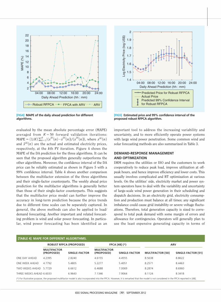
evaluated by the mean absolute percentage error (MAPE) averaged from K5 50 forward validation iterations: MAPE5 11/K 2g

Kk51 0 1x

1k2 1n 22x1k2 1n 22 / 1x

1k2 1n 22 0 , where x1k2 1n 2 and x1k2 1n 2 are the actual and estimated electricity prices, respectively, at the kth FV iteration. Figure 4 shows the MAPE of the DA prediction for the three algorithms. It can be seen that the proposed algorithm generally outperforms the other algorithms. Moreover, the confidence interval of the DA price can be reliably estimated as shown in Figure 5 with a 99% confidence interval. Table 4 shows another comparison between the multifactor extension of the three algorithms and their single-factor counterparts. The weekly ahead price prediction for the multifactor algorithms is generally better than those of their single-factor counterparts. This suggests that the multifactor price model can further improve the accuracy in long-term prediction because the price trends due to different time scales can be separately captured. In general, the above methods can also be applied to load/demand forecasting. Another important and related forecast-ing problem is wind and solar power forecasting. In particu-lar, wind power forecasting has been identified as an

important tool to address the increasing variability and uncertainty, and to more efficiently operate power systems with large wind power penetration. Some common wind and solar forecasting methods are also summarized in Table 3.

DEMAND-RESPONSE MANAGEMENT AND OPTIMIZATIONDRM requires the utilities or ISO and the customers to work cooperatively to reduce peak load, improve utilization at off-peak hours, and hence improve efficiency and lower costs. This usually involves complicated and RT optimization at various levels. On the utilities’ side, electricity market and power sys-tem operators have to deal with the variability and uncertainty of large-scale wind power generation in their scheduling and dispatch decisions. In an electricity grid, electricity consump-tion and production must balance at all times; any significant imbalance could cause grid instability or severe voltage fluctu-ations. Therefore, total generation capacity is sized to corre-spond to total peak demand with some margin of errors and allowance for contingencies. Operators will generally plan to use the least expensive generating capacity in terms of

04:001.4

1.5

1.6

Log

Ele

ctric

ity P

rice

(log

US

$)

1.7

1.8

1.9

2

08:00Daily Ahead Prediction (hh : mm)

12:00 16:00 20:00 24:00

Predicted Price for Robust RFPCAActual PricePredicted 99% Confidence Intervalfor Robust RFPCA

[FIG5] Estimated price and 99% confidence interval of the proposed robust RFPCA algorithm.

22

20

18

16

14

12

MA

PE

(%

)

10

8

6

4

2

04:00 08:00Daily Ahead Prediction (hh : mm)

12:00 16:00 20:00 24:00

Robust RFPCA FPCA with ARV ARV

[FIG4] MAPE of the daily ahead prediction for different algorithms.

[TABLE 4] MAPE FOR DIFFERENT ALGORITHMS.

ROBUST RFPCA (PROPOSED) FPCA [48] (*) ARV

MULTIFACTOR (PROPOSED) SINGLE-FACTOR

MULTIFACTOR (PROPOSED) SINGLE-FACTOR MULTIFACTOR [50] SINGLE-FACTOR [51]

ONE DAY AHEAD 4.2395 2.8240 4.6155 4.4555 8.5638 8.8622

ONE WEEK AHEAD 4.7792 5.4805 5.2277 5.4051 8.2571 8.4463

TWO WEEKS AHEAD 5.7729 6.6612 6.4688 7.0069 8.2874 8.6960

THREE WEEKS AHEAD 6.6033 6.9643 7.1346 7.9064 8.1124 8.3418

(*) For illustrative purpose, the proposed multifactor model is also incorporated into the FPCA. However, it is remarked that the model is not considered in the FPCA reported in [48].


marginal cost, and use additional capacity from more expensive plants as demand increases. In most cases, DR aims to reduce peak demand to reduce the risk of potential disturbances, avoiding additional capital investment for additional plants as well as avoiding the use of more expensive and/or less efficient operating plants. Another less common use of DR is to increase demand during periods of high supply and/or low demand to maintain grid stability. Energy storage such as pumped-storage hydroelectricity is another way to increase load during periods of low demand for use at later time. To get a better picture of the optimization involved, we briefly review the short-term operation of the power systems and markets in the United States and illustrate the concept with some simple examples later in the section “Utilities—The Unit Commitment Problem and Real-Time Pricing.”

In addition to the UC problem above, the operators have to collect and analyze RT network information and related events such as outages, voltage loss, and maintain a database of demand responsive resources. Depending on the sophistication of the control system, analysis of the demand responsive behavior and compliance with DR requests may have to be per-formed. Using this information, appropriate price and DR requests can be determined to meet the electricity load, while minimizing costs and observing stability, transmission capacity limitations and other physical constraints. We shall also illus-trate with a simple example the kind of optimization involved.

At the customer side, one has to response to dynamic pricing and make appropriate decisions possibly though optimization

approaches. As mentioned in the section “Smart Grid,” exam-ples of dynamic pricing include: RTP, PP, and TOU pricing. In [12], an open automated DR communications specifications (OpenADR) data model was developed to standardize DR com-munication from the utility or independent system operator (ISO) to commercial and industrial customers [55]. OpenADR is a Web services-based information model that supports all the pricing tariffs above to facilitate customers participating in automated DR programs with building control systems to use the price information as input to their building control systems and automate DR strategies. Alternatively, prices can be mapped into “building operation modes,” to be inputted to the building control systems. Mapping prices to operation modes may facili-tate wider customer participation since it simplifies their pro-cessing of dynamic pricing signals and carrier communications, allows compatibility with existing DR customers and their DR strategies, and allows interoperability with less-sophisticated or legacy controls. Typical characteristics of the pricing tariffs and short-term power market operation in the United States are also summarized in Table 5.

It comes as no surprise that dynamic pricing comes in dif-ferent forms, which also forms different business models for load control aggregation [11]. Due to the complicated pricing structure and the RT nature of the price, automated DR at the customer side using an EMS is highly desirable. The detailed optimization differs somewhat for smart home or commercial and industrial users. In the sections “Smart Home and DRM Optimization” and “Microgrid for Commercial and Industrial

[TABLE 5] DYNAMIC PRICING SCHEMES [12] AND OPERATIONS OF POWER MARKETS IN THE UNITED STATES [56].

RTPIN RTP, ELECTRICITY PRICES VARY CONTINUOUSLY THROUGHOUT THE DAY AT REGULARLY INTERVAL (USUALLY HOURLY) AS A FUNCTION OF ENVIRONMEN-TAL CONDITIONS (SUCH AS OUTDOOR AIR TEMPERATURE) OR ELECTRICITY SUPPLY AND DEMAND CONDITIONS. RT PRICES CAN BE SET DAY AHEAD (DA) OR DAY OF (DO) SCHEDULES. IN DA-RTP, PRICES ARE SET DA, WHICH TAKES EFFECT THE NEXT DAY, WHEREAS IN DO-RTP, PRICES ARE SET AT REGULAR INTERVAL, USUALLY EACH HOUR AND TAKES EFFECT THE SAME DAY.

PPIN PP, ELECTRICITY PRICES ON PEAK DAYS ARE DIFFERENT FROM ELECTRICITY PRICES ON NONPEAK DAYS. PRICES ARE GENERALLY PRESENT.

TOUIN TOU, CUSTOMERS KNOW THEIR ELECTRICITY PRICES MORE THAN A DAY IN ADVANCE, THOUGH THE PRICE VARIES THROUGHOUT THE DAY.

OPERATIONS OF POWER MARKETS IN THE UNITED STATESA1) DETERMINATION OF RESERVE REQUIREMENTS: OPERATING RESERVES ARE ALWAYS REQUIRED TO MAINTAIN RELIABILITY AND SECURITY OF POWER SYSTEMS. THEY CAN BE MAINLY CLASSIFIED INTO 1) REGULATING RESERVE, WHICH IS ASSISTED BY GENERATING UNITS WITH AUTOMATIC GENERATION CONTROL (AGC) TO PROVIDE INSTANTANEOUS RESPONSE TO THE CHANGE OF SYSTEM GENERATION DUE TO FREQUENCY DEVIATIONS AND 2) CONTINGEN-CY RESERVE WHICH NEEDS TO RESPONSE TO EMERGENCY CONDITIONS, SUCH AS FORCED OUTAGES OF GENERATORS ETC., WITHIN, SAY, TEN MINUTES. THE CONTINGENCY RESERVE CAN FURTHER BE DIVIDED INTO SPINNING AND NONSPINNING (SUPPLEMENTAL) RESERVE, IN WHICH AT LEAST 50% MUST BE SPINNING, WHICH MAY BE ADJUSTED DUE TO SEASONAL CHANGES.

A2) DA OPERATIONS: AFTER COLLECTING THE NECESSARY INFORMATION FROM THE MARKET PARTICIPANTS (E.G., THE ENERGY DEMAND, OPERATING RESERVE, UC CONSTRAINTS INCLUDING THE RAMPING RATES, START-UP COSTS/TIMES, MINIMUM UP/DOWN-TIME OF GENERATING UNITS, ETC), A TWO-STAGE PROCEDURE FOR THE CLEARING OF DA MARKET IS PERFORMED. THE FIRST STAGE INVOLVES THE SECURITY CONSTRAINED UC (SCUC) PROBLEM, WHICH AIMS TO MINIMIZE THE OPERATING COSTS WHILE MEETING THE TOTAL DEMAND BID INTO THE MARKET AS WELL AS THE UC CONSTRAINTS. USUAL-LY, THE RESULTING PROBLEM IS A MIXED INTEGER LINEAR PROGRAMMING (MILP) PROBLEM IN THE PRESENCE OF THE UC CONSTRAINTS AND TRANSMISSION CONSTRAINTS ARE SOMETIMES SIMPLIFIED OR OMITTED SO AS TO SOLVE THE PROBLEM IN A REASONABLE TIME. IN THE SECOND STAGE, A SECURITY CON-STRAINED ECONOMIC DISPATCH (SCEC) IS RUN SUBJECT TO THE TRANSMISSION CONSTRAINTS TO DERIVE THE LMPS FROM THE ENERGY BALANCE CON-STRAINTS IN EACH OF THE TRANSMISSION NODES GIVEN THE COMMITTED SCHEDULE OBTAINED FROM THE SCUC. NOTE THAT THE TRANSMISSION CONSTRAINTS IN SCED ARE SOMETIMES SIMPLIFIED IN LINEAR REPRESENTATION OR OMITTED SO THAT THE RESULTING LINEAR PROBLEM CAN BE SOLVED IN A REASONABLE TIME. THE CALCULATED LMP AND MARKET CLEARING PRICES FOR DIFFERENT RESERVES ARE THEN USED IN THE FINANCIAL SETTLEMENT OF THE DA MARKET. AFTER CLEARING THE DA MARKET, THE SYSTEM OPERATOR WILL PERFORM POST-DA RELIABILITY ASSESSMENT WITH SCUC USING THE PRE-DICTED LOADS.

A3) RT OPERATIONS: TO HANDLE POSSIBLY CHANGING OPERATING CONDITIONS (E.G., FORCED OUTAGES, DEVIATION FROM PREDICTED LOADS, ETC), THE RELIABILITY ASSESSMENT MAY BE REPEATED DURING THE OPERATING DAY. MEANWHILE, MARKET PARTICIPANTS CAN BID THEIR REMAINING RESOURCES IN THE RT MARKET. WITHIN THE OPERATING HOURS, THE SCED IS RUN TO DISPATCH THE SYSTEM AT A SHORT TIME INTERVAL (SAY, FIVE MINUTES IN MOST ISO/RTO MARKETS), WHILE RT PRICES FOR ENERGY (LMP) AND OPERATING RESERVES ARE CALCULATED.


Users,” we will review recent approaches to these problems, propose several new concepts and approaches, and give sever-al illustrations.

UTILITIES—THE UNIT COMMITMENT PROBLEM AND REAL-TIME PRICINGTo get some ideas about the UC problem, let us examine the typical short-term operation of power systems based on ISO/regional transmission organization (ISO/RTO) markets in the United States [56]. Then we will describe approaches for addressing the variable nature of wind and other renewable power in the UC problem. Moreover, we will illustrate how DR can be taken into account in the dispatch operations to achieve RTP.

OPERATION OF POWER SYSTEMS AND MARKETS IN THE UNITED STATESIn general, the operation includes 1) determination of reserve requirements, 2) DA operations, and 3) RT operations, which are summarized in Table 5. Currently, most intermittent resources such as wind power are not included in the DA oper-ations of most U.S. markets and are considered as price takers in the RT operations. It is expected that they will be integrated to the DA in the future. This poses a considerable problem as the variability and uncertainty of intermittent renewable resources may increase in a short time interval the amount of regulation reserves in the system. An excellent overview of the required reserves due to wind power is reported in [57]. Case studies also confirm that higher wind penetration will need higher degree of backup reserves, which varies from 1% to 2% to around 18%.

UNIT COMMITMENT PROBLEM AND PRICING WITH DEMAND RESPONSETo address the variability of wind power in UC problem, [58] focused on the risk brought by high wind penetration and developed a risk evaluation method for the short-term opera-tion of power systems. References [59] and [60] employed sto-chastic optimization to deal with the uncertainty of wind power in the UC problem (see Table 5). Since the pdf of the wind is not easy to obtain, [61] proposed a robust UC model with bounds on wind power generation to capture the inter-mittent nature of wind energy generation and to derive both the price levels and generator schedule based on DR. The posi-tive effect of DR in the form of RTP on better wind utilization was also studied in [7], where additional contingency reserve requirements and transmission constraints are considered. As

an illustration, we consider the UC problem with RTP-DR as follows:

minaNG

i51 aT

t511 gi xi,t1 ri yi,t1 ai zi,t 2

2 aT

t51dta

M

m51 wt, m pm 111 hm 2

s.t.aM

m51wt, m5 1, 4t; a

NG

i51xi, t1 vt5 dta

M

m51wt, m 111 hm 2 ,

4t;

aT

t51dta

M

m51 wt,m pm 111 hm 2 # b; yi,t, zi,t, wt,m5 50,16,

xi,t $ 0, 4i, t;

and the generators’ constraints in Table 6, where the discrete price model for the DR in the second term of the objective is adopted from [61]. There are M different price levels, and each of them is associated with an expected increase/decrease of the demand at different time instants. At each time instant t, the first constraint ensures that only one price level is selected, which is determined by the binary decision variables wt, m. With the chosen price level pm, the resulting demand 111 hm 2dt has to be met by the generation and wind powers, as described in the second constraint. The objective is to simultaneously minimize the generation cost and maintain the same revenue of the operator before the RTP DR is applied. To achieve the latter objective, the total revenue is bounded as in the third constraint. On the other hand, the generators’ parameters commonly considered in the UC problem are sum-marized as follows: gi, ri, and ai are respectively the genera-tion, running, and start-up costs, xi, t is the power generation level, yi, t and zi, t are binary decision variables, which deter-mine respectively the on/off status and turn-on status. The descriptions of generators’ constraints are summarized in Table 6 and interested readers are referred to [58]–[61] and references therein for more details. To demonstrate the idea of the UC problem with RTP DR, a simulation was carried out with the following settings: the DA hourly demand and the generators’ characteristics are extracted from [62], where NG5 36 thermal units are present. Moreover, according to the initial minimum up, minimum down, and start-up conditions given in [62], additional constraints (similar to those in the second column of Table 6 with t5 1) are also included in the problem. The total revenue before the RTP DR is set as B5 10. For illustrative purposes, we consider M5 9 the price levels and the corresponding demand increases/decreases are summarized in Table 7. In this framework, other realistic price-demand models such as [13] can also be used. The resulting MILP problem is solved using CPLEX Optimization

[TABLE 6] SUMMARY OF GENERATORS’ CONSTRAINTS.

MINIMUM UP 2 yi, t211 yi, t2 yi,h # 0

4i, t $ 2, h [ 3t, min 1b1i 1 t21, T2124

RAMPING UP xi, t11 # xi,t1 yi,t D1i 1 112 yi,t 2ui # 0,

4i, t5 1,...,T2 1

MINIMUM DOWN yi, t212 yi,t1 yi,h # 1

4i, t $ 2, h[ 3t, min 1b2i 1 t21,T21 24,

RAMPING DOWN xi,t # xi, t111 yi, t11 D2i 1 112yi, t11 2ui # 0

4i, t5 1, c,T21

START-UP OPERATION 2 yi, t211 yi,t2 zi,t # 0, 4i,t $ 2, GENERATION CAPACITY li yi, t # xi, t # ui yi, t, 4i, t,


Studio 12.3. Figure 6 shows how the determined price levels vary with the demand.

SMART HOME AND DRM OPTIMIZATIONNext we consider the optimization in a smart home, where most electric appliances (smart appliances) are networked together and are controlled by a home EMS as shown in Figure 2. On one side, utilities gather the information such as the consumers’ usage of electricity from the smart meters, and set the price level using, say, the RTP DR algorithm mentioned previously to reduce the peak electricity load. In response to the price signals, the customers can shift their demands automatically or manually with the help of the home EMS to the off-peak hours so as to minimize their electricity payment. To achieve this goal, the home EMS automatically predicts the electricity price and coordinates the operating schedule of smart appliances with the consent of the customers. As rooftop solar electric systems and small wind turbines are widely deployed, the customers may fur-ther harvest these free DERs through the automatic coordi-nation of the EMS. It is also envisioned that battery-assisted (BA) smart appliances or high-capacity battery storage devic-es (fuel cells) will get into the mainstream to allow better utilization of DERs. Moreover, smart appliances may have

the ability to reduce its power consumption by slightly com-promising their quality of services upon receiving the demand requests from the EMS.

We now briefly review approaches that have been put for-ward for solving the DR optimization problem and propose a new scheduling algorithm based on L1 regularization tech-nique. The main objective of DR optimization is to minimize the electricity bill or maximize their users’ satisfaction/comfort-ability by continually monitoring the electricity price informa-tion, allocating available resources and actively managing the load of appliances. A number of algorithms such as particle swarm optimization (PSO) [63], linear programming [64], and convex programming [65] have been proposed for DR optimiza-tion. Unlike the PSO and other heuristic algorithms that may result in premature convergence, the latter two convex pro-gramming approaches are more attractive because the problem can be solved efficiently using interior point methods and the optimality of the solution is guaranteed.

To carry out DR optimization, appropriate models for the appliances are usually required so that proper control (load, charging discharging storage) can be performed using the forecasted electricity price and model-based predicted energy consumption. Examples of these appliances include heating, ventilation, and air-conditioning systems [21], [22]. Another common cost model involved in DR optimization is called the utility function, which measures the users’ satisfaction on the appliances [65], [66]. This function is usually inversely propor-tional to the amount of energy consumed by the appliances so that the electricity cost can be reduced without significantly discomfort the users. In the convex optimization approach, these models are usually chosen as convex or concave func-tions to obtain an overall convex problem. In [65], the models of four common types of electric appliances in a household were discussed. The first type is concerned with the tempera-ture-related appliances such as heaters and ACs, the second is the schedule-based (SB) appliances such as plug-in hybrid electric vehicles and washers, the third is related to the essen-tial appliances such as lighting, and the final one is the enter-tainment appliances such as TVs, video games, and computers. Each type of the appliances is characterized by its own utility function U 1qt 2 that measures the user’s satisfaction on the power consumption qt at time t as well as the constraints of qt. For example, the concave utility function of Type 1 appliances is related to the inside temperature W in 1t 2 and the most com-fortable temperature Wcomf 1t 2 as UW 1W

in 1t 2 , W comf 1t 22 5c12c2 1W

in 1t 22W comf 1t 22 2 for some positive constants c1 and c2. This in turn can be expressed in terms of qt using the lin-ear dynamical model W in 1t 2 5W in 1t21 2 1 a 3W out 1t 2 2 W in 1t21 241 bqt, where a and b denote the thermal condition surrounding the appliance and W out 1t 2 is the outside tempera-ture. Moreover, additional constraints can be imposed on qt to specify respectively its operating and temperature ranges as Q # qt # Q and W comf # W in 1t 2 # W comf(E1).

However, the models of the aforementioned Types 2 and 4 appliances allow them to be switched off during operation

5,500

5,000

4,500

MW

hU

S$/

kW/h

4,000

3,500

0.8

0.6

0.4

0.2

02 4 6 8 10 12

Time (h)14 16 18 20 22 24

2 4 6 8 10 12

Price

Demand

14 16 18 20 22 24

[FIG6] Illustration of RTP-DR in the UC problem.

[TABLE 7] SUMMARY OF THE PRICE-DEMAND MODEL.

PM HM

0.13 7.9%

0.23 4.1%

0.33 1.7%

0.43 0.0%

0.53 21.4%

0.63 22.5%

0.73 23.5%

0.83 24.4%

0.93 25.1%


[65], which may not be reasonable in practice. In this tutorial, we assume that they should have to run until completion once started. More specifically, suppose that there are NS such SB appliances, and each of them has to complete its task within a user’s preferred time period t [ 3TS_i , TS_i 4 and has a known load profile ES_i

o 1t 2 for t [ 30, kS_i2 1 4, where kS_i is the total number of time slots for the task being completed. Therefore, there are Mi5 TS_i2 TS_i2 kS_i1 2 possible schedules and the scheduling problem is to select the best schedule in 5ES_i

o 1t2 TS_i2m 2 , m5 0, c, Mi21}, which depends on the price level within the user’s preferred time period. Alternatively, the load schedule can be written as ES_i 1t 2 5 gMi21

m50 a i,m ES_io 1t2TS_i2m 2 , where ai,m5 0, 1 is the

binary decision variable indicating that the schedule is select-ed when it is equal to one. To ensure that only one schedule is selected at a time, we further impose gMi

m51 a i, m5 1 (E2). We can see that the resulting scheduling problem is a com-binatorial problem. To solve this difficult problem, we first relax the binary decision variable ai, m to a real-valued vari-able as 0 # a i, m # 1, 4i, m (E3). Then, we minimize a L1 regularization term in the form of gMi

m51 0a i, m 0 so as to enforce the value of ai, m associated with the best schedule to be as large as possible, while keeping others as close to zero as possible. A major advantage is that the resulting problem is convex.

In addition to the above household appliances, we also con-sider an appliance equipped with internal batteries, called BA appliances. Suppose that there are NA such appliances, each of them containing an internal battery that has a charging/dis-charging power of bi,t at time t. Its ability of charging 1bi, t . 0 2 or discharging 1bi, t , 0 2 offers additional to handle the inter-mittent renewable energy sources and improves the response to RTP. Following the battery model in [65], the constraints RB_i # bi,t # RB_i and 0 # g t

t51 bi,t # Bi

(E4) are imposed to restrict the maximum charging rate (RB_i . 0), max-imum discharging rate (RB_i , 0), and maximum capacity (Bi). Also, to model the possible damage against the bat-tery’s lifetime, the term Fi 1bi,t2 5hi,1 bi, t

2

2hi, 2 bi,t bi, t111 hi,3 min 1bi,t2hi,4 Bi, 0 22,

for some positive constants hi, k, k5 1, 2, 3, 4, is added to the cost func-tion. On the other hand, we assume that each appliance of this type consumes a power of EA_i 1t 2 and allows direct control DR up to DDC_i EA_i 1t 2 at time t, where DDC_i is the maximum possible percent-age reduction in load. Therefore, the actual DR of the ith appliance at time t, di, t, is bounded by 0 # di,t # DDC_i (E5). Similar to previous discussion, we also include a convex function, Gi 1di, t 2 5

l1 1DDC_i2 di,t1l2 22l3, in the objective

to measure user’s dissatisfaction for some positive constants lk, k5 1, 2, 3.

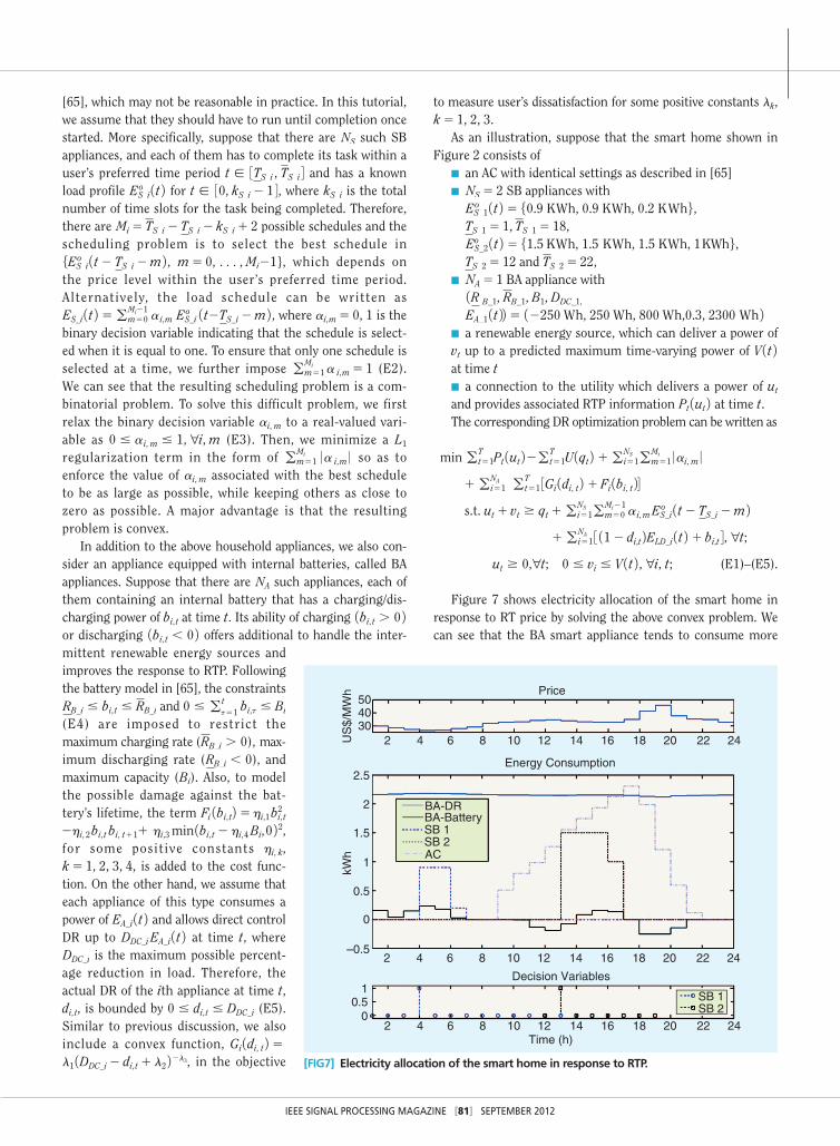
As an illustration, suppose that the smart home shown in Figure 2 consists of

■ an AC with identical settings as described in [65] ■ NS5 2 SB appliances with

ES_1o 1t 2 5 50.9 KWh, 0.9 KWh, 0.2 KWh6,

TS_15 1, TS_15 18, ES_2

o 1t 2 5 51.5 KWh, 1.5 KWh, 1.5 KWh, 1 KWh6, TS_25 12 and TS_25 22,

■ NA5 1 BA appliance with 1R B_1, RB_1, B1, DDC_1, EA_1 1t 22 5 12250 Wh, 250 Wh, 800 Wh,0.3, 2300 Wh 2

■ a renewable energy source, which can deliver a power of vt up to a predicted maximum time-varying power of V 1t 2 at time t

■ a connection to the utility which delivers a power of ut and provides associated RTP information Pt 1ut 2 at time t. The corresponding DR optimization problem can be written as

min gTt51Pt 1ut 22g

Tt51U 1qt 2 1 gNS

i51gMi

m51 0ai, m 0

1 gNA

i51 gTt51 3Gi 1di, t 2 1 Fi 1bi, t 24

s.t. ut1 vt $ qt1 gNS

i51gMi21m50 a i, m ES_i

o 1t2 TS_i2m 2

1 gNA

i51 3 112 di,t 2ELD_i 1t 2 1 bi,t 4, 4t;

ut $ 0,4t; 0 # vi # V 1t 2 , 4i, t; (E1)–(E5).

Figure 7 shows electricity allocation of the smart home in response to RT price by solving the above convex problem. We can see that the BA smart appliance tends to consume more

504030

2.5

Price

2 4 6 8 10

Energy Consumption

12 14 16 18 20 22 24

2 4 6 8 10

Decision Variables

Time (h)

12 14 16 18 20 22 24

2 4 6 8 10 12 14 16 18 20

SB 1SB 2

22 24

2

1.5

1

0.5

0

–0.5

10.5

0

US

$/M

Wh

kWh

SB 1SB 2AC

BA-BatteryBA-DR

[FIG7] Electricity allocation of the smart home in response to RTP.


power and its internal battery is charged up in the case of lower price. Moreover, for the SB appliances, the best schedule with the lowest price within the user’s preferred period can be select-ed. Here, we note that the Karush-Kuhn-Tucker conditions of the above DR optimization problem suggest that its solution is usually sparse. Also, the largest nonzero coefficient, which may not be exactly equal to one depending on the form of the price and utility functions, tends to indicate the most cost-effective schedule corresponding to the largest cost reduction. This is indicated in the lowest part of Figure 7, where the relaxed deci-sion variables corresponding to the best schedules can be easily singled out. Such schedule will be considered as the solution of target scheduling problem before the relaxation in (E3).

MICROGRID FOR COMMERCIAL AND INDUSTRIAL USERSAs mentioned earlier in the section “Smart Grid,” microgrids improve reliability and PQ, allow higher penetration of renew-

able sources and dynamic islanding, and simplify the control of the grid. If heat generation is required, the use of waste heat through cogeneration or combined cooling heat and power (CCHP) can deliver both electricity and useful heat from an energy source such as natural gas. In [67], the problem of optimal control of DERs with DR under electricity and fuel price uncertainty is studied. Given uncertain electricity and fuel prices modeled by the commonly used mean-reverting (OU) processes [46], a weighted average of the expected annual energy costs and CO2 emissions of the microgrid for various capacity sizes is minimized. The problem is solved via Monte Carlo simulation and dynamic programming (DP) since the discount cost is used for meeting energy loads over a number of test years. Using this stochastic DP (SDP) method, different policies such as doing nothing, DERs with DR and DERs with-out DR can be compared with different emphasis on costs and CO2 emission. It was found that DERs dominates the case of doing nothing in terms of lower expected energy bills, reduced

Tertiary Control

Secondary Control

Measurements

Ka

refa

Kr

refr

refp

refd

reff

Kp

Kf

Kd

Turbine Air Conditioners

Refrigerator

Pump

Controller

Wind Turbine

Controller

PV Generator

Uncontrollable Load

Microgrid

EV EV

Aggregator

Flywheel

Regulating

Battery Storage

Water Heater

Diesel Governor

Signal

Regulating

Signal

Regulating

Signal

+

+

+

+

+

–

–

–

–

–

–

[FIG8] Frequency regulation on a microgrid.


CO2 emissions, and lower condition value-at-risk (cVAR). Moreover, DR makes DERs more attractive, especially when the electricity price becomes more uncertain. It was also found that large distributed generator (DG) unit performs the best in terms of the environment aspect in minimizing CO2 emissions and medium DG units give the lowest expected cost. This shows the usefulness of microgrids with DER and DR in cost reduction and reducing CO2 emissions. An important problem, however, is how to control in RT the microgrids under RTP so as to minimize electricity costs and possibly CO2 emission and how to exercise DR. This is an optimal control problem that can be solved using approximate dynamic pro-gramming (ADP) [68]. An alternative approach using a formu-lation similar to the home EMS described in “Smart Home

and DRM Optimization” can also be developed [69]. This approach can also be extended to the power management of an electric vehicle charging station [69]. Next we present some results on the improved frequency regulation of microgrids.

FREQUENCY REGULATION OF MICROGRIDSIn traditional power systems, frequency deviation, which is an indicator of instantaneous imbalance of supply and demand of electricity, is regulated with a hierarchical control framework. The large variation of high wind power penetration poses sig-nificant challenges to the traditional load-following frequency regulation methodology, especially for microgrids operating in isolated mode. As the smart grid is equipped with state-of-the-art communication and control technologies, the load response provides a novel approach to balance power systems. By a comprehensive framework with demand and generation as described above, the traditional frequency regulation meth-odology will be shifted to a novel generation/load-following methodology. The appropriateness of this match has been rec-ognized by the Electric Reliability Council of Texas (ERCOT), which allows load curtailment to supply half of ERCOT’s 2,300 MW spinning reserve requirement. The PJM Interconnection also recently changed its reliability rules to allow loads to sup-ply spinning reserve [70]. Potential resources for load response include ACs, refrigerators, freezers, pumps, electric hot water heaters, washing machines and dryers, storage systems, plug-in electric vehicles, and lighting. For a microgrid, an alterna-tive scheme for frequency regulation may be employed as illustrated in Figure 8 [70], where a wind generator works together with the loads with load response. For example, with wind power output and total load in Figure 9, the frequencies of the microgrid with/without load response are illustrated in Figure 10. It can be seen that the load response also improves significantly the controllability of the microgrid.

ACKNOWLEDGMENTSThis work was supported in part by the National Basic Research Program (2012CB215102) and General Research Fund of Hong Kong Research Grant Council under projects 7124/10E and 7124/11E.

AUTHORSS.C. Chan ([email protected]) received the B.Sc. (Eng) and Ph.D. degrees from The University of Hong Kong, Pokfulam, in 1986 and 1992, respectively. Since 1994, he has been with the Department of Electrical and Electronic Engineering, the University of Hong Kong, where he is currently a professor. His research interests include fast transform algorithms, filter design and realization, multirate and biomedical signal process-ing, communications and array signal processing, high-speed A/D converter architecture, bioinformatics, image-based render-ing, and the smart grid. He is currently a member of the Digital Signal Processing Technical Committee of the IEEE Circuits and Systems Society, and he is an associate editor of Journal of Signal Processing Systems and IEEE Transactions on Circuits

0.8

0.6

0.4

0.2

0

3.4

3.2

3

0 100 200Time (s)

300 400 500

0 100 200Time (s)

(b)

(a)

300 400 500Win

d P

ower

(p.

u.)

Tot

al L

oad

(p.u

.)

[FIG9] (a) Output of a wind generator and (b) total load in a microgrid.

[FIG10] Frequency deviation (a) without load response and (b) with load response.

0–0.4

–0.2

df (

%)

df (

%)

0

0.2

0.4

–0.4

–0.2

0

0.2

0.4

100 200Time (s)

Time (s)

(a)

(b)

300 400 500

0 100 200 300 400 500


and Systems II. He was the chair of the IEEE Hong Kong Chapter of Signal Processing in 2000–2002, an organizing com-mittee member of the 2003 IEEE International Conference on Acoustics, Speech, and Signal Processing, the 2010 International Conference on Image Processing. He was an asso-ciate editor of IEEE Transactions on Circuits and Systems I from 2008 to 2009. He is a Member of the IEEE.

K.M. Tsui ([email protected]) received the B.Eng., M.Phil., and Ph.D. degrees in electrical and electronic engineer-ing from the University of Hong Kong, in 2001, 2004, and 2008, respectively. He is currently working as postdoctoral fel-low in the Department of Electrical and Electronic Engineering at the same university. His main research inter-ests are in array signal processing; high-speed AD converter architecture; biomedical signal processing; digital signal pro-cessing; multirate filter bank and wavelet design; and digital filter design, realization, and application.

H.C. Wu ([email protected]) received the B.Eng. degree in electrical engineering from the University of New South Wales, Australia, in 2008 and the M.Sc degree in electri-cal and electronic engineering from the University of Hong Kong in 2009. He is currently a Ph.D. student in the Department of Electrical and Electronic Engineering at the University of Hong Kong. His main research interests are in pattern recognition, bioinformatics, digital signal processing, and time-series analysis.

Yunhe Hou ([email protected]) received his B.E. (1999) and Ph.D. (2005) degrees from Huazhong University of Science and Technology, China. He worked as a postdoctoral research fellow at Tsinghua University from 2005 to 2007. He was a visiting scholar at Iowa State University and a research scientist at University College Dublin, Ireland, from 2008 to 2009. He was also a visiting scientist with the Laboratory for Information and Decision Systems, Massachusetts Institute of Technology, Cambridge in 2010. He is currently an assistant professor at the University of Hong Kong. He is a Member of the IEEE.

Yik-Chung Wu ([email protected]) received the B.Eng. degree in electrical and electronic engineering in 1998 and the M.Phil. degree in 2001 from the University of Hong Kong. He received the Ph.D. degree from Texas A&M University, College Station, in 2005. From 2005 to 2006, he was with the Thomson Corporate Research, Princeton, New Jersey, as a member of technical staff. He has been an assistant professor at the University of Hong Kong since 2006. He was a visiting scholar at Princeton University in 2011. His research interests are in general area of signal processing and communication systems. He is currently an associate editor of IEEE Communications Letters.

Felix F. Wu ([email protected]) is the Philip Wong Wilson Wong Professor in electrical engineering at the University of Hong Kong, where he served as pro vice chancellor (vice presi-dent) from 1997 to 2001. He is also a Professor Emeritus at the University of California, Berkeley, where he has been on the faculty since 1974. He is a Fellow of the IEEE.

REFERENCES[1] J. Conti and G. E. Sweetnam, “Emissions of greenhouse gases in the Unit-ed States 2008,” U.S. Energy Information Administration, U.S. Dept. Energy, Washington, DC, Tech. Rep. DOE EIA-0573(2008), Dec. 2009.

[2] M. Glinkowski, J. Hou, and G. Rackliffe, “Advances in wind energy technolo-gies in the context of smart grid,” Proc. IEEE, vol. 99, no. 6, pp. 1083–1097, June 2011.

[3] K. Turitsyn, P. Sulc, S. Backhaus, and M. Chertkov, “Options for control of reactive power by distributed photovoltaic generators,” Proc. IEEE, vol. 99, no. 6, pp. 1063–1073, June 2011.

[4] N. P. Padhy, “Unit commitment—A bibliographical survey,” IEEE Trans. Power Syst., vol. 2, no. 19, pp. 1196–1205, 2004.

[5] DOE. (2008, July). 20% wind energy by 2030: Increasing wind energy’s con-tribution supply. U.S. Dept. Energy, Office of Energy Efficiency and Renewable [Online]. Available: http://www1.eere.energy.gov/windandhydro/wind_2030.html

[6] P. Denholm and R. M. Margolis, “Evaluating the limit of solar photovolta-ics (PV) in traditional electric power systems,” Energy Policy, vol. 35, no. 6, pp. 2852–2861, 2007.

[7] R. Sioshansi and W. Short, “Evaluating the impacts of real-time pricing on the usage of wind generation,” IEEE Trans. Power Syst., vol. 24, no. 2, pp. 516–524, May 2009.

[8] R. H. Lasseter, “Smart distribution: Coupled microgrids,” Proc. IEEE, vol. 99, no. 6, pp. 1074–1082, June 2011.

[9] J. Wells, Electricity Markets—Consumers Could Benefit From Demand Programs, But Challenges Remain. Washington , DC: Government Accountability Office, 2004.

[10] G. W. Arnold, “Challenges and opportunities in smart grid: A position ar-ticle,” Proc. IEEE, vol. 99, no. 6, pp. 922–927, 2011.

[11] S. S. Oren, “Demand response: A historical perspective and business models for load control aggregation,” presented at the Power System Engineering Re-search Center Public Webinar, Feb. 1, 2011.

[12] G. Ghatikar, J. L. Mathieu, M. A. Piette, and S. Liliccote. (2010, Dec. 1–3). Open automated demand response technologies for dynamic pricing and smart grid. presented at Grid-Interop Conference 2010, Chicago, IL. [Online]. Avail-able: http://drrc.lbl.gov/sites/drrc.lbl.gov/files/lbnl-4028e.pdf

[13] A. Faruqui and S. Sergici, “Household response to dynamic pricing of elec-tricity: A survey of 15 experiments,” J. Regulatory Economics, vol. 38, no. 2, pp. 193–225, Oct. 2010.

[14] D. Kathan, C. Daly, E. Eversole, M. Farinella, J. Gadani, R. Irwin, C. Lankford, A. Pan, C. Switzer, and D. Wight, “National action plan on demand response,” The Federal Energy Regulatory Commission Staff, Federal Energy Regulatory Commission, Washington, DC, Tech. Rep. AD09-10, 2010.

[15] C. King. (2010). PowerCentsDC program final report. Smart Meter Pilot Program, Inc., eMeter Corp. Washington, DC, USA. [Online]. Available: http://www.powercentsdc.org/ESC%2010-09-08%20PCDC%20Final%20Report%20-%20FINAL.pdf

[16] “What Is the Smart Grid?” SmartGrid.gov. U.S. Dept. of Energy. [Online]. Available: www.smartgrid.gov/the_smart_grid#home

[17] A. G. Phadke, “Synchronized phasor measurements in power systems,” IEEE Comput. Appl. Power, vol. 6, no. 2, pp. 10–15, Apr. 1993.

[18] A. Gomez-Exposito, A. Abur, A. de la Villa Jaen, and C. Gomex-Quiles, “A multilevel state estimation paradigm for smart grids,” Proc. IEEE, vol. 99, no. 6, pp. 952–976, June 2011.

[19] M. H. J. Bollen, I. Y. H. Gu, S. Santoso, M. F. Mcgranaghan, P. A. Crossley, M. V. Ribeiro, and P. F. Ribeiro, “Bridging the gap between signal and power,” IEEE Signal Process. Mag., vol. 26, no. 4, pp. 12–31, July 2009.

[20] H. Gharavi and R. Ghafurian, “Smart grid: The electric energy system of the future,” Proc. IEEE, vol. 99, no. 6, pp. 917–921, June 2011.

[21] H. Sane and M. Guay, “Minimax dynamic optimization over a finite-time horizon for building demand control,” in Proc. 2008 American Control Conf., Seattle, WA, June 11–13, 2008, pp. 1469–1474.

[22] D. Bargiotas and J. D. Birdwell, “Residential air conditioner dynamic model for direct load control,” IEEE Trans. Power Delivery, vol. 3, no. 4, pp. 2119–2126, 1988.

[23] Y. C. Ho and R. C. K. Lee, “A Bayesian approach to problems in stochas-tic estimation and control,” IEEE Trans. Automat. Contr., vol. AC-9, no. 4, pp. 333–339, 1964.

[24] D. L. Alspach and H. W. Sorenson, “Nonlinear Bayesian estimation using Gaussian sum approximation,” IEEE Trans. Automat. Contr., vol. AC-17, no. 4, pp. 439–448, Aug. 1972.

[25] R. E. Kalman, “A new approach to linear filtering and prediction problems,” Trans. ASME, J. Basic Eng., vol. 82D, pp. 35–45, Mar. 1960.

[26] A. P. Dempster, N. M. Laird, and D. B. Rubin, “Maximum likelihood from incomplete data via the EM algorithm,” J. Roy. Statist. Soc. B, vol. 39, no. 1, pp. 1–38, 1977.

[27] R. Tibshirani, “Regression shrinkage and selection via the lasso,” J. Roy. Statist. Soc. B, vol. 58, no. 1, pp. 267–288, 1996.


[28] J. Fan and R. Li, “Variable selection via nonconcave penalized likelihood and its oracle properties,” J. Amer. Stat. Assoc., vol. 96, no. 456, pp. 1348–1360, Dec. 2001.

[29] S. C. Chan, Z. G. Zhang, and Y. J. Chu, “A new transform-domain regu-larized recursive least M-estimate algorithm for robust linear estimation,” IEEE Trans. Circuits Syst. II, vol. 58, no. 2, pp. 120–128, Feb. 2011.

[30] P. J. Huber, Robust Statistics. New York: Wiley, 1981.

[31] C. J. Masreliez and R. D. Martin, “Robust Bayesian estimation for the linear model and robustifying the Kalman filter,” IEEE Trans. Automat. Contr., vol. AC-22, pp. 361–371, June 1977.

[32] S. C. Chan and Y. Zou, “A recursive least M-estimate algorithm for robust adaptive filtering in impulsive noise: Fast algorithm and convergence perfor-mance analysis,” IEEE Trans. Signal Processing, vol. 52, no. 4, pp. 975–991, Apr. 2004.

[33] A. Doucet, N. De Freitas, and N. J. Gordon. Sequential Monte Carlo Methods in Practice. New York: Springer-Verlag, 2001.

[34] S. C. Chan, B. Liao, and K. M. Tsui, “Bayesian Kalman filtering, regulariza-tion and compressed sampling,” in Proc. IEEE MWSCAS, Aug. 2011, pp 1–4.

[35] S. Haykin, Adaptive Filter Theory, 4th ed. Englewood Cliffs, NJ: Prentice-Hall, 2001.

[36] J. Fan and I. Gijbels, Local Polynomial Modelling and its Applications. London, U.K.: Chapman & Hall, 1996.

[37] V. Katkovnik, “A new method for varying adaptive bandwidth selection,” IEEE Trans. Signal Processing, vol. 47, no. 9, pp. 2567–2571, Sept. 1999.

[38] Z. G. Zhang, S. C. Chan, K. L. Ho, and K. C. Ho, “On bandwidth selection in local polynomial regression analysis and its application to multi-resolution analy-sis of non-uniform data,” J. Signal Process. Syst., vol. 52, no. 3, pp. 263–280, Sept., 2008.

[39] S. C. Chan and Z. G. Zhang, “Local polynomial modeling and variable band-width selection for time-varying linear systems,” IEEE Trans. Instrum. Meas., vol. 60, no. 3, pp. 1102–1117, Mar. 2011.

[40] Z. G. Zhang and S. C. Chan, “Tracking of voltage flicker in power distribu-tion systems: A local polynomial modeling approach,” in Proc. ICGCS, Shanghai, China, June 21–23, 2010, pp. 543–548.

[41] Z. G. Zhang and S. C. Chan, “A new regularized adaptive windowed lomb periodogram for spectral analysis of time-varying signals with impulsive compo-nents,” submitted for publication.

[42] R. Weron, Modeling and Forecasting Electricity Loads and Prices: A Statistical Approach. West Sussex, England: Wiley, 2006.

[43] Y. Hou, C. C. Liu, and H. Salazar, “Electricity prices as stochastic processes,” in Advances in Electric Power and Energy (Power Engineering Series of IEEE Press/Wiley books), M. El Hawary, Ed., to be published.

[44] Z. Xia, Pricing and Risk Management in Competitive Electricity Markets, Ph.D. dissertation, School of Industrial and System Engineering, Georgia Inst. Technol., 2005.

[45] Y. Hou and Y. He, “Modeling of electricity prices,” in Proc. 2010 Int. Conf. Green Circuits and Systems, 21–23 June, 2010, pp. 549–554.

[46] Y. Hou and F. Wu, “Probability distribution functions of generator profit from spot market,” in Proc. 2008 16th Power Systems Computation Conf., pp. 1261–1266, 2008.

[47] R. Huisman and R. Mahieu, “Regime jumps in electricity prices,” Energy Economics, vol. 25, no. 5, pp. 425–434, 2003.

[48] H. L. Shang. (2010). Nonparametric modeling and forecasting electricity de-mand: An empirical study, in Proc. Australian Statistical Conf. [Online]. Avail-able: http://www.buseco.monash.edu.au/ebs/pubs/wpapers/2010/wp19-10.pdf

[49] B. Yang, “Projection approximation subspace tracking,” IEEE Trans. Signal Processing, vol. 43, no. 1, pp. 95–107, Jan. 1995.

[50] S. C. Chan, H. C. Wu, and K. M. Tsui, “Robust recursive eigen-decomposi-tion and subspace-based algorithms with application to fault detection in wireless sensor networks,” IEEE Trans. Instrum. Meas., vol. 61, no, 6, pp. 1703–1718, 2012.

[51] C. Y. Fung and S. C. Chan, “Estimation of fast fading channel in impulse noise environment,” in Proc. IEEE Int. Symp. Circuits and Systems (ISCAS), AZ, May 26–29, 2002, vol. 4, pp. 497–500.

[52] Y. He, “Modeling electricity prices for generation investment and scheduling analysis,” Ph.D. dissertation, Dept. Elect. Eng., Hong Kong Univ., Hong Kong, China, 2010.

[53] S. Heydari and A. S. Siddiqui, “Valuing a gas-fired power plant: A com-parison of ordinary linear models, regime switching approaches, and models with stochastic volatility,” Energy Economics, vol. 32, no. 3, pp. 709–725, Oct. 2009.

[54] ISO New England Inc. (2011). Hourly zonal information. [Online]. Avail-able: http://www.iso-ne.com/markets/hstdata/znl info/hourly/index.html

[55] M. A. Piette, S. Kiliccote, and G. Ghatikar. “Design and implementation of an open, interoperable automated demand response infrastructure,” presented at the Grid Interop Forum, Albuquerque, NM, Nov. 2007, Paper LBNL-63665.

[56] A. Botterud, J. Wang, V. Miranda, R. Bessa, H. Keko, and J. S. Akilimali, “Wind power forecasting and electricity market operations,” presented at the IAWind 2010 Conf., Ames, IA, Apr. 6, 2010.

[57] H. Holttinen, P. Meibom, A. Orths, B. Lange, M. O’Malley, J. O. Tande, A. Estanqueiro, E. Gomez, L. Söder, G. Strbac, J. C. Smith, and F. van Hulle, “Impacts of large amounts of wind power on design and operation of power sys-tems, results of IEA collaboration,” Wind Energy, vol. 14, no. 2, pp. 179–192, Mar. 2011.

[58] X. Li and C. Jiang, “Unit commitment and risk management based on wind power penetrated system,” in Proc. Int. Conf. Power System Technology, 2010, pp. 1–7.

[59] A. Tuohy, P. Meibom, E. Denny, and M. O’Malley, “Unit commitment for systems with significant wind penetration,” IEEE Trans. Power Syst., vol. 24, no. 2, pp. 592–601, 2009.

[60] J. Wang, M. Shahidehpour, and Z. Li, “Security-constrained unit commit-ment with volatile wind power generation,” IEEE Trans. Power Syst., vol. 23, no. 3, pp. 1319–1327, 2008.

[61] L. Zhao and B. Zeng. (2010). Robust unit commitment problem with de-mand response and wind energy. Univ. South Florida, Tech. Rep. [Online]. Avail-able: http://www.optimization-online.org/DB_HTML/2010/11/2784.html

[62] H. Ma and S. M. Shahidehpour, “Unit commitment with transmission secu-rity and voltage constraints,” IEEE Trans Power Syst., vol. 14, no. 2, pp. 757–764, 1999.

[63] M. A. A. Pedrasa, T. D. Spooner, and I. F. MacGill, “Coordinated scheduling of residential distributed energy resources to optimize smart home energy ser-vices,” IEEE Trans. Smart Grid, vol. 1, no. 2, pp. 134–143, Sept. 2010.

[64] A. Mohsenian-Rad and A. Leon-Garcia, “Optimal residential load control with price prediction in real-time electricity pricing environments,” IEEE Trans. Smart Grid, vol. 1, no. 2, pp. 120–133, Sept. 2010.

[65] N. Li, L. Chen, and S. H. Low, “Optimal demand response based on util-ity maximization in power networks,” in Proc. IEEE Power and Energy Society General Meeting, July 2011, pp. 1–8.

[66] P. Samadi, A. Mohsenian-Rad, R. Schober, V. W. S. Wong, and J. Jatskev-ich, “Optimal real-time pricing algorithm based on utility maximization for smart grid,” in Proc. IEEE Int. Conf. Smart Grid Communications, 2010, pp. 415–420.

[67] A. Siddiqui, M. Stadler, C. Marnay, and J. Lai, “Optimal control of distrib-uted energy resources and demand response under uncertainty,” in Proc. Int. Association for Energy Economics, June 6–9, 2010.

[68] R. N. Anderson, A. Boulanger, W. B. Powell, and W. Scott, “Adaptive sto-chastic control for the smart grid,” Proc. IEEE, vol. 99, no. 6, pp. 1098–1115, June 2011.

[69] K. M. Tsui, S. C. Chan, and Y. Hou, “Demand response optimization for microgrids and electric vehicle station under real-time pricing,” Dept. Elect. Electron. Eng., Hong Kong Univ., Hong Kong, P.R. China, Internal Rep., 2011.

[70] M. Ilic, N. Popli, J. Y. Joo, and Y. Hou, “Possible engineering and economic framework for implementing demand side participation in frequency regulation at value,” presented at IEEE PES General Meeting, 2011.

[71] H. Gharavi and B. Hu, “Multigate communication network for smart grid,” Proc. IEEE, vol. 99, no. 6, pp. 1028–1045, 2011.

[72] S. Galli, A. Scaglione, and Z. Wang, “For the grid and through the grid: The role of power line communications in the smart grid,” Proc. IEEE, vol. 99, no. 6, pp. 998–1027, June 2011.

[73] R. Samsudin, A. Shabri, and P. Saad, “A comparison of time series forecast-ing using support vector machine and artificial neural network model,” J. Appl. Sci., vol. 10, no. 11, pp. 950–958, 2010.

[74] T. Niimura, “Forecasting techniques for deregulated electricity market prices—Extended survey,” in Proc. IEEE PES Power Systems Conf. Exposition, (PSCE 2006), Oct. 2006, pp. 51–56.

[75] B. Ernst, B. Oakleaf, M. L. Ahlstrom, M. Lange, C. Moehrlen, B. Lange, U. Focken, and K. Rohrig, “Predicting the wind,” IEEE Power Energy Mag., vol. 5, no. 6, pp. 78–89, Nov. 2007.

[76] H. Zheng and A. Kusiak, “Prediction of wind farm power ramp rates: A data-mining approach,” J. Solar Energy Eng., vol. 131, no. 3, pp. 031011-1–031011-8, 2009.

[77] F. Deng, G. Su, C. Liu, and Z. Wang, “Global solar radiation modeling using the artificial neural network technique,” in Proc. IEEE Power and Energy Engi-neering Conf., Apr. 2010, pp. 1–5.

[78] A. Kudish and E. Evseev, “The assessment of four different correction mod-els applied to the diffuse radiation measured with a shadow ring using global and normal beam radiation measurements for Beer Sheva,” Solar Energy, vol. 82, no. 2, pp. 144–156, 2008.

[79] F. Deng, G. Su, C. Liu, and Z.Wang, “Prediction of solar radiation resources in China using the LS-SVM algorithms,” in Proc. IEEE ICCAE, Apr. 2010, pp. 31–35.

[SP]

Documents

W OTO.COM/© SIGAL SUHLER MORAN - Department of Electrical and