VSC-HVDC transmission line fault location based on

ARCHIVES OF ELECTRICAL ENGINEERING VOL. 70(2), pp. 381 –398 (2021)

DOI 10.24425/aee.2021.136991

VSC-HVDC transmission line fault location based ontransient characteristics

YANXIA ZHANG, ANLU BIo , JIAN WANG, FUHE ZHANG, JINGYI LU

School of Electrical and Information Engineering, Tianjin UniversityChina

e-mail: [email protected]

(Received: 14.09.2020, revised: 22.12.2020)

Abstract:Accurate and reliable fault location is necessary for ensuring the safe and reliableoperation of the VSC-HVDC transmission system. This paper proposed a single-terminalfault location method based on the fault transient characteristics of the two-terminal VSC-HVDC transmission system. The pole-to-pole transient fault process was divided into threestages, the time-domain expression of the DC current during the diode freewheel stagewas used to locate the fault point, and a criterion for judging whether the fault evolves tothe diode freewheel stage was proposed. Taking into account the enhancing effect of theopposite system to the fault current, theDC side pole-to-ground fault networkwas equated toa fourth-order circuit model, the relationship of fault distance with the characteristic roots offault current differential equationwas derived, and the Prony algorithmwas utilized for data-fitting to extract characteristic roots to realize fault location. A two-terminal VSC-HVDCtransmission system was modelled in PSCAD/EMTDC. The simulation result verifies thatthe proposed principle can accurately locate the fault point on the VSC-HVDC transmissionlines.Key words: characteristic roots, fault location, identification of fault stages, Prony algo-rithm, VSC-HVDC

1. Introduction

With the development of power electronics technology, voltage source converter-based highvoltage direct current (VSC-HVDC) technology has made rapid progress. VSC-HVDC adoptsbidirectional controllable power electronic devices, can control both active and reactive powersimultaneously, is suitable for long-distance power transmission, distributed energy interconnec-tion, power grid interconnection, and other fields [1, 2]. However, high voltage direct current

0

© 2021. The Author(s). This is an open-access article distributed under the terms of the Creative Commons Attribution-NonCommercial-NoDerivatives License (CCBY-NC-ND4.0, https://creativecommons.org/licenses/by-nc-nd/4.0/), which per-mits use, distribution, and reproduction in any medium, provided that the Article is properly cited, the use is non-commercial,and no modifications or adaptations are made.

https://orcid.org/0000-0003-0249-0165

mailto:[email protected]

https://creativecommons.org/licenses/by-nc-nd/4.0/

382 Yanxia Zhang et al. Arch. Elect. Eng.

(HVDC) transmission lines have relatively high fault possibility because of the complex geo-graphical environment and poor working conditions, and are difficult to manual inspect due to thefast reaction of protection and the inapparent external fault performance. Therefore, the researchon VSC-HVDC transmission line fault location is of great theoretical significance and practicalvalue for improving the reliability of the power system.

The existing VSC-HVDC transmission line fault location method can be divided into threecategories [3, 4]: the traveling wave method [5–9], the natural frequency method [10–12], andthe fault analysis method [14–18]. The traveling wave method locates the fault point accordingto the relationship among the traveling wave arrival time at the direct current (DC) bus, trav-eling wave velocity, and the fault distance. In order to extract the traveling wave arrival timeat the DC bus, the wavelet transform is applied in [8], it can effectively extract the charac-teristics of the fault traveling wave and eliminate the impact of dispersion, but the extractionaccuracy is affected by the transform scale. In order to obtain a relatively accurate wave veloc-ity, reference [9] utilizes the distributed traveling wave detection device to detect the travelingwave propagation time for a transmission line of known length, then the wave velocity can becalculated, but the distributed traveling wave detection device increases the cost. The naturalfrequency refers to a series of harmonic components that constitute the fault transient travelingwave spectrum, among them, the harmonic component with the lowest frequency and the largestamplitude is the dominant natural frequency. The natural frequency method located the faultpoint according to the functional relationship between the dominant natural frequency and thefault distance, it does not need to detect the traveling wave head. And the precise extractionof the dominant natural frequency is the key to locate accurately. For this reason, the multi-ple signal classification algorithm is applied to extract the dominant natural frequency in [12].Reference [13] combined the natural frequency method and the traveling wave method, it usesthe former to roughly detect the fault area, then uses the latter to accurately find out the ar-rival time of the traveling wave head. This method not only avoids the dead zone of the naturalfrequency method, but also improves the fault location accuracy. The fault analysis methodconstructs the equivalent equations according to the relationship between system parametersand the measured electric quantity, then locates the fault point by solving the equations. Ref-erences [16] and [17] calculate the voltage distributions along the transmission lines from theboth side measurements, then locate the fault point according to the principle that the voltagedistribution difference at the fault point is the smallest. The key factor affecting the accuracyof the fault analysis method is the accuracy of the line model. The adopted transmission linemodel in [16] is the Bergeron model and that in [17] is the distributed parameter model whichtakes the multi-order distance infinitesimal into account. The former line model is less accurate,the latter is more accurate but the multi-order infinitesimal increases the calculation amount.Reference [18] analyzes the fault characteristics of pole-to-pole and pole-to-ground fault onVSC-HVDC transmission lines, and calculates the fault distance by the voltage reference com-parison method. But it’s affected by the transition resistance and the accuracy needs to be furtherimproved.

Aiming at the two-terminal VSC-HVDC transmission system, this paper proposes a singleended fault location principle based on the transient characteristics analysis of the pole-to-poleand pole-to-ground fault. For the pole-to-pole fault, this paper divides the fault transient processinto three stages, and utilizes the time-domain expression of DC current at the diode freewheel

Vol. 70 (2021) VSC-HVDC transmission line fault location 383

stage to realize the fault location, and gives the identification criterion for judging whether thefault evolves to the diode freewheel stage. For the pole-to-ground fault, this paper takes the currentfrom the opposite system into account, and derives the differential equation of the fault current.The fault distance and transition resistance are solved as the expression of the characteristic rootsof the differential equation. Then the extended Prony algorithm is used to fit the data to extractthe characteristic roots. The simulation results under PSCAD/EMTDC show that the accuracy ofthe proposed fault location principle meets the engineering requirement.

2. Analysis of transient characteristics of VSC-HVDC transmission fault

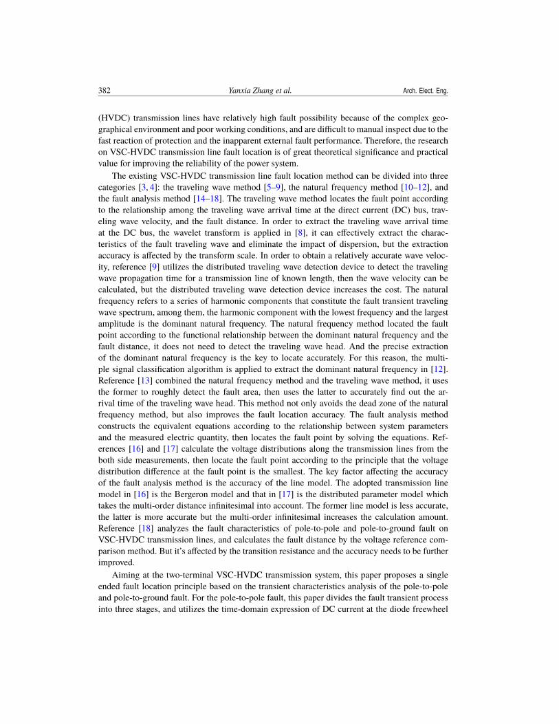
Since the conventional HVDC systems mostly adopt two-terminal structure, the two-terminalVSC-HVDC transmission system is analyzed in this paper. As is shown in Fig. 1, the VSC-HVDCsystem consists of converter stations at both sides and bipolar transmission lines, the connectingtransformers are connected in Ynd, that is, the neutral point of the transformer grid side winding isdirectly earthed. This connection can cut off the zero-sequence current propagation path betweenthe alternating current (AC) side and DC side. The neutral point of the DC side capacitor is alsoearthed to form symmetrical positive and negative DC transmission lines to reduce the insulationlevel of the DC line to ground.

Transformer

VSC1 VSC2

Transformer

Fig. 1. Typical earthing mode of two-terminal VSC-HVDC

2.1. Analysis of pole-to-pole fault transient characteristics

The pole-to-pole fault is the most serious fault of VSC-HVDC transmission lines. The shortcircuit current will rise to several times the rated current within a few milliseconds, and will causea huge impact on insulated gate bipolar transistors (IGBT).

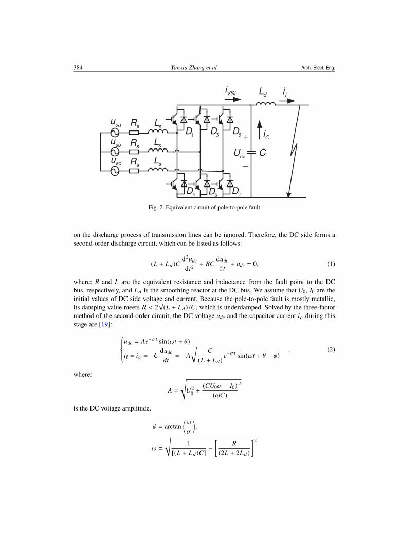
The Fig. 2. shows the equivalent circuit of the pole-to-pole fault. The two-level VSC consistsof six IGBTs and the freewheeling diodes D1~D6 connected in antiparallel, and C is the DC sideparallel capacitor. The IGBT can be instantaneously blocked after fault occurs due to its self-protection function. However, the anti-parallel diode is still connected to form a circuit betweenthe AC system, DC side and the fault point, thus the DC side fault cannot be completely isolated.The fault transient process is analyzed below.

1. Capacitor discharge stageAfter a pole-to-pole fault occurs on the transmission lines, during the initial stage, the DC

side voltage udc is greater than the AC side line voltage, the parallel capacitor begins to dischargethrough the DC lines and the smoothing reactor. So, the influence of distributed capacitance


CCi

li

dcU

sau

sbu

scu

sR sL

VSIi

sR

sR

sL

sL

2D4D

+

–

1D 3D 5D

6D

dL

Fig. 2. Equivalent circuit of pole-to-pole fault

on the discharge process of transmission lines can be ignored. Therefore, the DC side forms asecond-order discharge circuit, which can be listed as follows:

(L + Ld)Cd2udc

dt2 + RCdudc

dt+ udc = 0, (1)

where: R and L are the equivalent resistance and inductance from the fault point to the DCbus, respectively, and Ld is the smoothing reactor at the DC bus. We assume that U0, I0 are theinitial values of DC side voltage and current. Because the pole-to-pole fault is mostly metallic,its damping value meets R < 2

√(L + Ld)/C, which is underdamped. Solved by the three-factor

method of the second-order circuit, the DC voltage udc and the capacitor current ic during thisstage are [19]:

udc = Ae−σt sin(ωt + θ)

il = ic = −Cdudc

dt= −A

√C

(L + Ld)e−σt sin(ωt + θ − φ)

, (2)

where:

A =

√U2

0 +(CU0σ − I0)

(ωC)

2

is the DC voltage amplitude,

φ = arctan(ω

σ

),

ω =

√1

[(L + Ld)C]−

[R

(2L + 2Ld)

]2


is the frequency of DC voltage and current,

σ =R

[2 (L + Ld)]

is the attenuation coefficient,

θ = arctan[

UoωC(CUoσ − Io)

].

From Equation (2), it can be seen that the capacitor discharge stage is a second-order un-derdamped oscillation process, and the DC side current will gradually oscillate and decay. Thechanging trend of the DC side voltage and current are mainly determined by the resistance andinductance values in the fault loop. The larger the resistance value and the smaller the inductancevalue, the higher the oscillation frequency and the faster the attenuation rate.

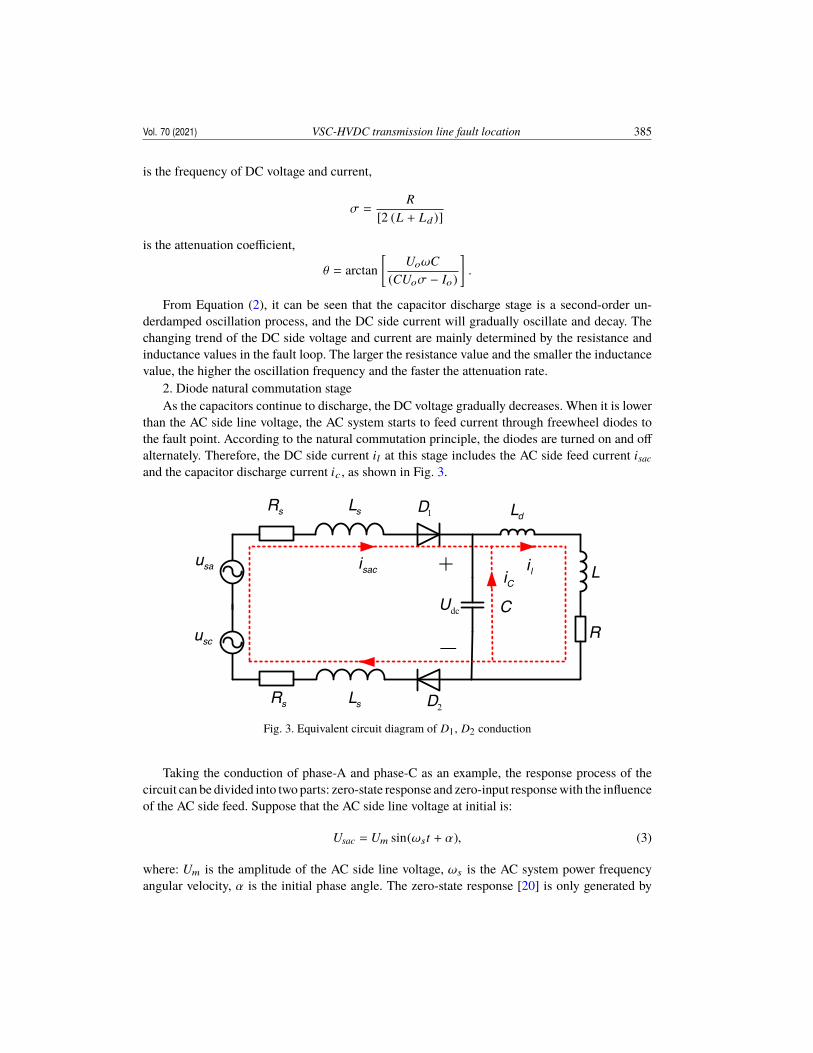
2. Diode natural commutation stageAs the capacitors continue to discharge, the DC voltage gradually decreases. When it is lower

than the AC side line voltage, the AC system starts to feed current through freewheel diodes tothe fault point. According to the natural commutation principle, the diodes are turned on and offalternately. Therefore, the DC side current il at this stage includes the AC side feed current isacand the capacitor discharge current ic , as shown in Fig. 3.

sau

1DsR sL

L

RCdcU

+

－

saci

2DsR sL

liCi

scu

dL

Fig. 3. Equivalent circuit diagram of D1, D2 conduction

Taking the conduction of phase-A and phase-C as an example, the response process of thecircuit can be divided into two parts: zero-state response and zero-input responsewith the influenceof the AC side feed. Suppose that the AC side line voltage at initial is:

Usac = Um sin(ωst + α), (3)

where: Um is the amplitude of the AC side line voltage, ωs is the AC system power frequencyangular velocity, α is the initial phase angle. The zero-state response [20] is only generated by


the external excitation source usac, and the DC side current component ilzs of the zero-stateresponse is:

ilzs = A sin (ωst + α − ϕ) , (4)where:

A =Um

√M2 + N2

is the magnitude of the fault component,

ϕ = arctan M/N

is the angle at which the fault component lags usac,

M = ωsLs

[1 − ω2

sC(L + Ld)]+ ωsCRRs + ωs (L + Ld),

N = R + ωsLsCR − Rs

[1 − ω2

sCL + Ld)].

The zero-input response is produced by the original energy storage of the inductance andcapacitance. According to the characteristics of the circuit, the differential equation is

di3lzi

dt3 + A1di2

lzi

dt2 + A2dilzidt+ A3 = 0, (5)

where: ilzi is the DC current component in the zero-input response, the coefficients are ex-pressed as:

A1 =[Rs (Ld + L) + Ls + R]

(LsL), A2 =

(2RsCR + 2Ls + Ld + L)(2LsLC)

, A3 =(R + Rs)2LsLC

.

Substituting the above coefficient expression into Formula (5), according to Shengjin’s for-mula, the characteristic roots of the differential equation are judged to consist of negative realroots and a pair of conjugate complex roots.

Therefore, the DC side current at this stage is superimposed of three kinds of components:the synchronous frequency sine component, the attenuated non-periodic component and theattenuated free oscillation periodic component.

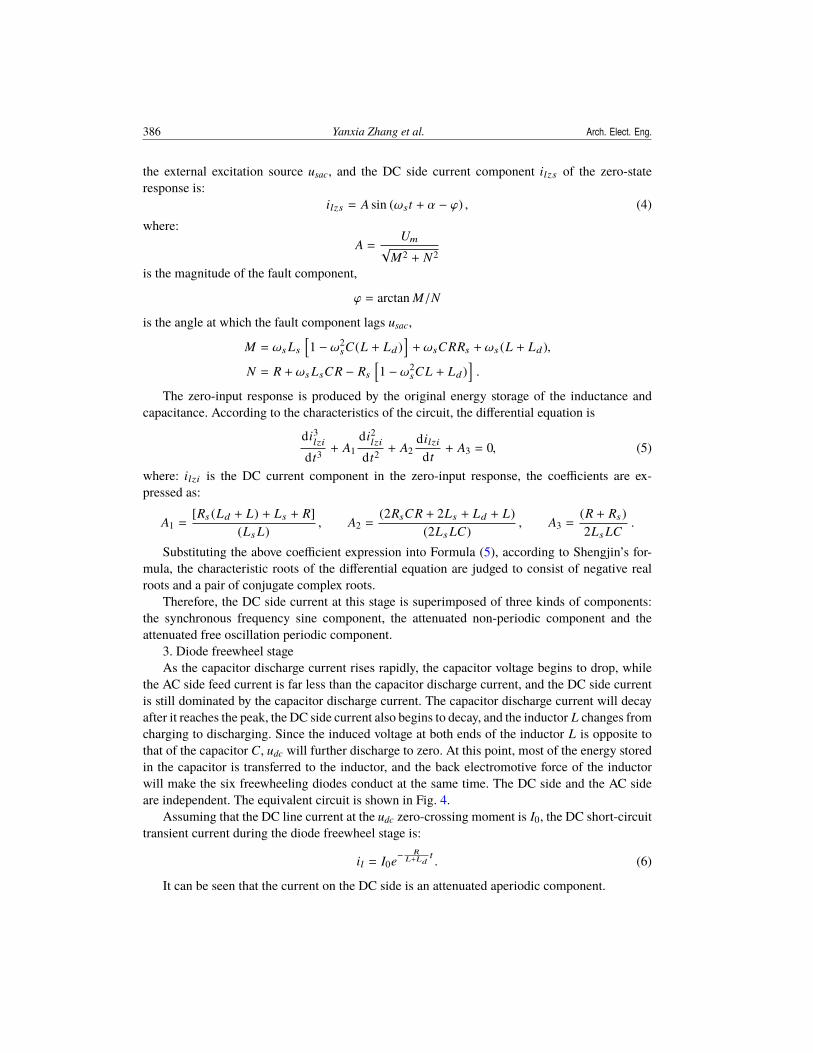
3. Diode freewheel stageAs the capacitor discharge current rises rapidly, the capacitor voltage begins to drop, while

the AC side feed current is far less than the capacitor discharge current, and the DC side currentis still dominated by the capacitor discharge current. The capacitor discharge current will decayafter it reaches the peak, the DC side current also begins to decay, and the inductor L changes fromcharging to discharging. Since the induced voltage at both ends of the inductor L is opposite tothat of the capacitor C, udc will further discharge to zero. At this point, most of the energy storedin the capacitor is transferred to the inductor, and the back electromotive force of the inductorwill make the six freewheeling diodes conduct at the same time. The DC side and the AC sideare independent. The equivalent circuit is shown in Fig. 4.

Assuming that the DC line current at the udc zero-crossing moment is I0, the DC short-circuittransient current during the diode freewheel stage is:

il = I0e−R

L+Ldt. (6)

It can be seen that the current on the DC side is an attenuated aperiodic component.


sau

sbu

scu

sR sLsai 1D

3D

5D

2D

6D

4Dsbi

sci1D 3D 5D

2D6D4D

dLli

sR sL

sR sLR

L

(a) (b)

Fig. 4. Equivalent circuit of diode freewheel stage: DC side (a); AC side (b)

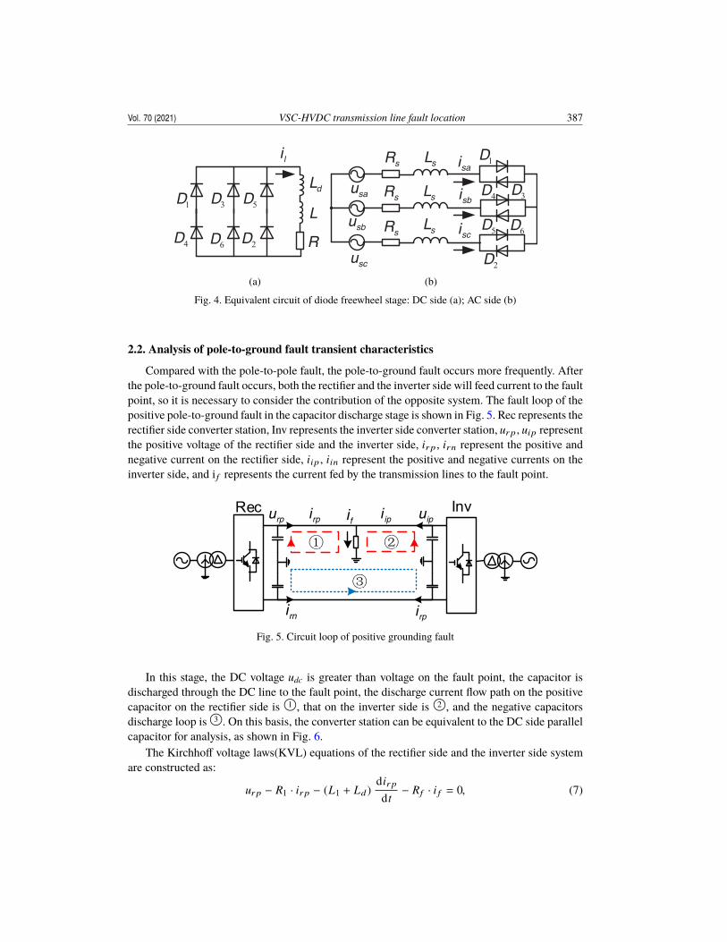
2.2. Analysis of pole-to-ground fault transient characteristics

Compared with the pole-to-pole fault, the pole-to-ground fault occurs more frequently. Afterthe pole-to-ground fault occurs, both the rectifier and the inverter side will feed current to the faultpoint, so it is necessary to consider the contribution of the opposite system. The fault loop of thepositive pole-to-ground fault in the capacitor discharge stage is shown in Fig. 5. Rec represents therectifier side converter station, Inv represents the inverter side converter station, urp , uip representthe positive voltage of the rectifier side and the inverter side, irp , irn represent the positive andnegative current on the rectifier side, iip , iin represent the positive and negative currents on theinverter side, and i f represents the current fed by the transmission lines to the fault point.

① ②

③

Rec Invrpu rpi fi ipi ipu

rpirniFig. 5. Circuit loop of positive grounding fault

In this stage, the DC voltage udc is greater than voltage on the fault point, the capacitor isdischarged through the DC line to the fault point, the discharge current flow path on the positivecapacitor on the rectifier side is 1O, that on the inverter side is 2O, and the negative capacitorsdischarge loop is 3O. On this basis, the converter station can be equivalent to the DC side parallelcapacitor for analysis, as shown in Fig. 6.

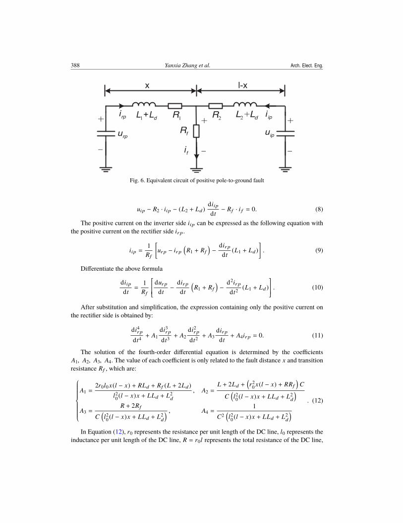
The Kirchhoff voltage laws(KVL) equations of the rectifier side and the inverter side systemare constructed as:

urp − R1 · irp − (L1 + Ld)dirpdt− Rf · i f = 0, (7)


+

—

+

—

+

—

x l-x

2 + dL L2R1Rrpi

rpu fRipi

ipu

fi

1+ dL L

Fig. 6. Equivalent circuit of positive pole-to-ground fault

uip − R2 · iip − (L2 + Ld)diipdt− Rf · i f = 0. (8)

The positive current on the inverter side iip can be expressed as the following equation withthe positive current on the rectifier side irp .

iip =1

Rf

[urp − irp

(R1 + Rf

)−

dirpdt

(L1 + Ld)]. (9)

Differentiate the above formula

diipdt=

1Rf

durpdt−

dirpdt

(R1 + Rf

)−

d2irpdt2 (L1 + Ld)

. (10)

After substitution and simplification, the expression containing only the positive current onthe rectifier side is obtained by:

di4rpdt4 + A1

di3rpdt3 + A2

di2rpdt2 + A3

dirpdt+ A4irp = 0. (11)

The solution of the fourth-order differential equation is determined by the coefficientsA1, A2, A3, A4. The value of each coefficient is only related to the fault distance x and transitionresistance Rf , which are:

A1 =2r0l0x(l − x) + RLd + Rf (L + 2Ld)

l20 (l − x)x + LLd + L2

d

, A2 =L + 2Ld +

(r2

0 x(l − x) + RRf

)C

C(l20 (l − x)x + LLd + L2

d

)A3 =

R + 2Rf

C(l20 (l − x)x + LLd + L2

d

) , A4 =1

C2(l20 (l − x)x + LLd + L2

d

) . (12)

In Equation (12), r0 represents the resistance per unit length of the DC line, l0 represents theinductance per unit length of the DC line, R = r0l represents the total resistance of the DC line,


L = l0l represents the inductance of the DC line, Ld is the smoothing reactance at the DC outletof the converter station, and l is the total length of the DC line.

The Appendix verifies that the characteristic root discriminant of Equation (11) is above zero,so the solution of the differential equation consists of a pair of conjugate complex roots and twodifferent real roots [21]. The irp can be expressed as:

irp (t) = C1eλi t + C2eλ2t + C3eαt sin βt + C4eαt cos βt, (13)

where: C1eλi t , C2eλ2t are the attenuate aperiodic components, λ1, λ2 represent the attenuationcoefficients; C3eαt sin βt, C4eαt cos βt represent the damped free oscillation period component,α is the attenuation constant, β is the free oscillation angular frequency, corresponding to a pairof conjugate complex roots of the characteristic equation λ3,4 = αk ± i βk .

3. Method of fault location

3.1. Pole-to-pole fault location principle3.1.1. Identification of different fault stages

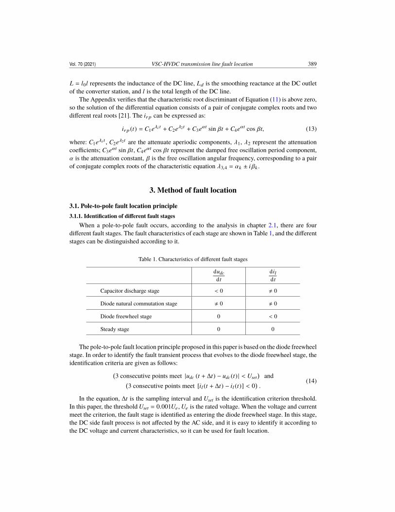
When a pole-to-pole fault occurs, according to the analysis in chapter 2.1, there are fourdifferent fault stages. The fault characteristics of each stage are shown in Table 1, and the differentstages can be distinguished according to it.

Table 1. Characteristics of different fault stages

dudcdt

dildt

Capacitor discharge stage < 0 , 0

Diode natural commutation stage , 0 , 0

Diode freewheel stage 0 < 0

Steady stage 0 0

The pole-to-pole fault location principle proposed in this paper is based on the diode freewheelstage. In order to identify the fault transient process that evolves to the diode freewheel stage, theidentification criteria are given as follows:(

3 consecutive points meet |udc (t + ∆t) − udc(t) | < Uset)

and(3 consecutive points meet [il (t + ∆t) − il (t)] < 0

).

(14)

In the equation, ∆t is the sampling interval and Uset is the identification criterion threshold.In this paper, the threshold Uset = 0.001Ue, Ue is the rated voltage. When the voltage and currentmeet the criterion, the fault stage is identified as entering the diode freewheel stage. In this stage,the DC side fault process is not affected by the AC side, and it is easy to identify it according tothe DC voltage and current characteristics, so it can be used for fault location.


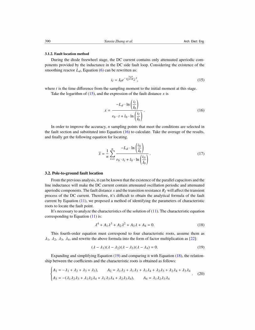
3.1.2. Fault location methodDuring the diode freewheel stage, the DC current contains only attenuated aperiodic com-

ponents provided by the inductance in the DC side fault loop. Considering the existence of thesmoothing reactor Ld , Equation (6) can be rewritten as:

il = I0e−r0x

l0x+Ldt, (15)

where t is the time difference from the sampling moment to the initial moment at this stage.Take the logarithm of (15), and the expression of the fault distance x is

x =−Ld · ln

(ilI0

)r0 · t + l0 · ln

(ilI0

) . (16)

In order to improve the accuracy, n sampling points that meet the conditions are selected inthe fault section and substituted into Equation (16) to calculate. Take the average of the results,and finally get the following equation for locating.

x =1n

n∑i=1

−Ld · ln(

iliI0

)r0 · ti + l0 · ln

(iliI0

) . (17)

3.2. Pole-to-ground fault locationFrom the previous analysis, it can be known that the existence of the parallel capacitors and the

line inductance will make the DC current contain attenuated oscillation periodic and attenuatedaperiodic components. The fault distance x and the transition resistance Rf will affect the transientprocess of the DC current. Therefore, it’s difficult to obtain the analytical formula of the faultcurrent by Equation (11), we proposed a method of identifying the parameters of characteristicroots to locate the fault point.

It’s necessary to analyze the characteristics of the solution of (11). The characteristic equationcorresponding to Equation (11) is:

λ4 + A1λ3 + A2λ

2 + A3λ + A4 = 0. (18)

This fourth-order equation must correspond to four characteristic roots, assume them asλ1, λ2, λ3, λ4, and rewrite the above formula into the form of factor multiplication as [22]:

(λ − λ1)(λ − λ2)(λ − λ3)(λ − λ4) = 0. (19)

Expanding and simplifying Equation (19) and comparing it with Equation (18), the relation-ship between the coefficients and the characteristic roots is obtained as follows:

A1 = −λ1 + λ2 + λ3 + λ3), A2 = λ1λ2 + λ1λ3 + λ1λ4 + λ2λ3 + λ2λ4 + λ3λ4

A3 = −(λ1λ2λ3 + λ1λ2λ4 + λ1λ3λ4 + λ2λ3λ4), A4 = λ1λ2λ3λ4. (20)


Substitute Equation (12) into Equation (20), the transition resistance Rf and fault distance xare obtained as:

Rf = −1

2C

(1λ1+

1λ2+

1λ3+

1λ4

)−

r0l2, (21)

x1,2 =l2±

12l0

(4L2

d + l20l2 + 4l0lLd −

4λ1λ2λ3λ4C2

) 12

. (22)

The fault distances solved by Equation (22) have two roots x1, x2 (x1 < x2), which aresymmetric about the midpoint of the line. In order to eliminate the false root, the differencebetween the calculated voltage and the actual measured voltage is used. Name the initial end ofthe line as M (rectifier side) and the terminal as N (inverter side). We assumed that the voltage atthe distance x from the initial end be u(x, t), and the current at the initial end be iM . According tothe equation of the uniform transmission line, the voltage at the beginning uM can be obtained by:

uM =u(x, t) + iM Zc sinh γx

cosh γx, (23)

where:

Zc =

√(r0 + jωl0)

(G0 + jωC0),

γ =√

(r0 + jωl0)(G0 + jωC0) ,

r0, l0, G0 and C0 are, respectively, the resistance, inductance, conductance and capacitance perunit line length, ω is the frequency corresponding to the characteristic roots λ3, λ4.

Substitute x2 into Equation (7) to obtain the calculated voltage at the fault point.

u f x2 = i f Rf = urp − R0 · x2 · irp − (L0 · x2 + Ld)dirpdt

. (24)

Then, substitute u f x2 into Equation (23) to replace u(x, t) to obtain the calculated voltage atthe exit of the rectifier side.

uMx2 =u f x2 + iM Zc sinh γx2

cosh γx2. (25)

When the real fault distance is x2, the calculated fault uMx2 and the actual measured valueuM are equal. When the real fault distance is x1, the calculated voltage uMx2 and the actualmeasured value uM are not equal. Therefore, by comparing the calculated voltage value with theactual measured voltage value, a simple and reliable criterion for identifying the false root of faultdistance is proposed as follows:

|uMx2 − uM | > Krel · 5%UN . (26)

Determine the actual fault points as x1 when consecutive points meet (26).There,UN is the rated value of DC voltage, Krel = 1.15 is the reliability coefficient. When the

calculated value uMx2 of port voltage and the actual value uM meet the above criteria, determinethe actual fault point as x1; otherwise, determine the actual fault point as x2.


The key of fault location is to accurately obtain λ1, λ2, λ3, λ4 from the sampling data. Theestimation model of the extended Prony algorithm has good adaptability to the fault currentrepresented in Equation (13), and the use of the extended Prony algorithm can effectively avoidthe iterative problem caused by the nonlinear solution. So, this paper uses the extended Pronyalgorithm to fit the sampling data and calculate the characteristic roots.

Assume that there are N measured data x(n), n = 0 ∼ N − 1, the extended Prony algorithmestimation model x(n) in discrete time form is:

x(n) =p∑i=1

Aieαin∆t cos (2π f in∆t + θi) =p∑i=1

bi zni , (27)

where:

bi = Ai exp[jθi

],

zi = exp[(αi + j2π f i)∆t

],

p is the order of the model; Ai , f i , θi , αi are the amplitude, frequency, initial phase angle andattenuation factor;∆t is the sampling interval. References [23,24] presented the numerical methodfor solving the four characteristic parameters. Combined with Equation (27), the characteristicroots λi (i = 1, 2, 3, 4) in Equation (13) are:

λi = αi + i2π f i = ln |zi | /∆t + arctan [Im(zi)/Re(zi)] /2π∆t . (28)

4. Simulation and verification

4.1. Parameters and oscillograms of simulationA two-terminal VSC-HVDC transmission system has been modelled in PSCAD/EMTDC.

The rectifier side adopts constant active power and constant reactive power control, the inverterside adopts constant DC voltage and constant AC voltage control. The parameters of HVDCtransmission systems are listed in Table 2. A data sampling frequency of 5 kHz is adopted, andthe data is imported into MATLAB for verification.

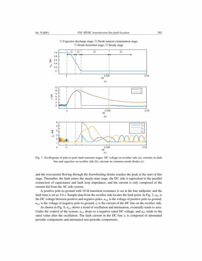
The pole-to-pole fault is set at the midpoint of the DC line (100 km), and the fault time is setas 2.0 s. The simulation oscillogram is shown in Fig. 7 below.

Fig. 7 shows that the transient process of the pole-to-pole fault consists of four stages: thecapacitor discharge stage, diode natural commutation stage, the diode freewheel stage and steadystage. During the capacitor discharge stage, the DC voltage drops while the fault current increasesrapidly, the current flowing through the freewheeling diodes is zero, and fault current is onlyprovided by the parallel capacitor discharge current on the DC side. When the DC voltage dropsto the AC side voltage, the AC side system starts to feed current into the fault point, and the faulttransient process enters the diode free commutation stage. Once the DC voltage drops to zero,the back electromotive force of the inductor will make the six freewheeling diodes conduct at thesame time, the DC side and the AC side are independent, so the fault transient process will enterthe diode freewheeling stage, the fault current is only provided by the inductance on the DC side,


1O Capacitor discharge stage; 2O Diode natural commutation stage;3O Diode freewheel stage; 4O Steady stage

00.20.40.60.81.0

t/s

① ② ③ ④

2 2.05

t/s

cili

2 2.05

024681012

0

1

23

4

56

2 2.05

/u d

cpu

/i D

kA

t/s

/ikA

1DI3DI5DI

2.025

2.025

2.025

(a)

(b)

(c)

Fig. 7. Oscillogram of pole-to-pole fault transient stages: DC voltage on rectifier side (a); currents in faultline and capacitor on rectifier side (b); currents in common-anode diodes (c)

and the overcurrent flowing through the freewheeling diodes reaches the peak at the start of thisstage. Thereafter, the fault enters the steady-state stage, the DC side is equivalent to the parallelconnection of capacitance and fault loop impedance, and the current is only composed of thecurrent fed from the AC side system.

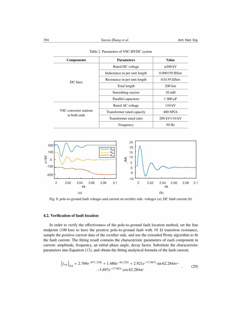
A positive pole-to-ground with 10 Ω transition resistance is set at the line midpoint, and thefault time is set as 2.0 s. Sample data from the rectifier side locates the fault point. In Fig. 2, udc isthe DC voltage between positive and negative poles, urp is the voltage of positive pole-to-ground,urn is the voltage of negative pole-to-ground, il is the current of the DC line on the rectifier side.

As shown in Fig. 8, urp shows a trend of oscillation and attenuation, eventually tends to zero.Under the control of the system, urn drops to a negative rated DC voltage, and udc tends to therated value after the oscillation. The fault current in the DC line il is composed of attenuatedperiodic components and attenuated non-periodic components.


Table 2. Parameters of VSC-HVDC system

Components Parameters Value

DC lines

Rated DC voltage ±200 kV

Inductance in per unit length 0.000159 H/km

Resistance in per unit length 0.0139 Ω/km

Total length 200 km

Smoothing reactor 10 mH

Parallel capacitors 1 000 µF

VSC converter stationsat both ends

Rated AC voltage 110 kV

Transformer rated capacity 400 MVA

Transformer rated ratio 200 kV/110 kV

Frequency 50 Hz

2 2.02 2.04 2.06 2.08 2.1

-200

-100

0

100

200dcurpurnu

t/s

-10

-505

10152025

2 2.02 2.04 2.06 2.08 2.1t/s

l/kA/

ukV

(a) (b)

Fig. 8. pole-to-ground fault voltages and current on rectifier side: voltages (a); DC fault current (b)

4.2. Verification of fault location

In order to verify the effectiveness of the pole-to-ground fault location method, set the linemidpoint (100 km) to have the positive pole-to-ground fault with 10 Ω transition resistance,sample the positive current data of the rectifier side, and use the extended Prony algorithm to fitthe fault current. The fitting result contains the characteristic parameters of each component incurrent: amplitude, frequency, an initial phase angle, decay factor. Substitute the characteristicparameters into Equation (13), and obtain the fitting analytical formula of the fault current.

irp

kA= 2.769e−871.150t + 1.480e−44.325t + 2.921e−17.967t sin 62.284πt−

−3.697e−17.967t cos 62.284πt. (29)


The four characteristic roots of the characteristic equation can be obtained by substituting αi

and f i into Equation (28).

λ1 = −871.150; λ2 = −44.325; λ3,4 = −17.967 ± i62.284π . (30)

Substitute l0 = 0.000159 mH, Ld = 10 mH, l = 200 km, C = 1000 µF and the abovecharacteristic roots into Equation (22), the fault distance is solved as follows:

x1,2 =l2±

12l0

(4L2

d + l20l2 + 4l0lLd −

4λ1λ2λ3λ4C2

) 12

=

= 100 ± 3144.65 ·(0.00268 −

4000000871.150 · 44.325 · (17.9672 + 62.2842π2)

) 12

.

(31)

The two solutions of the fault distance are:

x1 = 98.427, x2 = 101.572. (32)

According to the criterion in Equation (26), x1 is the real root of the fault distance.Table 3 lists the results of characteristic roots fitted by the extended Prony algorithm of the

pole-to-ground fault.

Table 3. The characteristic results of roots extracted by extended Prony algorithm of pole-to-ground fault

Fault distance/km Transitionresistance/Ω λ1 λ2 λ3,4

1 –901.290 –48.921 −106.850 ± 193.391i

10 10 –1171.235 –44.289 −134.865 ± 202.884i

100 –1114.264 –49.329 −22.570 ± 195.701i

1 –604.871 –63.843 −186.406 ± 62.121i

100 10 –871.150 –44.325 −17.967 ± 195.671i

100 –779.621 –49.552 −21.537 ± 195.263i

1 –901.287 –48.938 −106.847 ± 193.358i

190 10 –1169.861 –44.057 −13.486 ± 202.873i

100 –1112.071 –49.377 −22.461 ± 195.722i

The error of location is calculated by the following equation:

error =|calculated fault distance − real fault distance|

total length× 100%. (33)

Change the fault types, fault distance and the value of the transition resistance, the faultlocation results are shown in Table 4.

The results of the fault location show that the method proposed in this paper can avoid theinfluence of transition resistance effectively in the case of the pole-to-ground fault, and accuratefault location can be realized at both the near and far end of the DC bus.


Table 4. Fault location results

Fault Fault Transition Locating errortype distance/km resistance/Ω distance/km %

10Metallic

10.161 0.081

Pole-to-pole 100short circuit

100.181 0.090

190 190.165 0.083

1 9.683 0.159

10 10 10.055 0.028

100 10.609 0.305

1 101.415 0.708

Pole-to-ground 100 10 98.427 0.787

100 101.476 0.738

1 190.324 0.162

190 10 189.270 0.365

100 189.178 0.411

5. Conclusion

This paper proposed a simple and reliable method for the pole-to-pole fault according towhich the time-domain expression of the DC current during the diode freewheel stage was usedto locate the fault point, and the identification criterion for judging whether the fault evolves to thediode freewheel stage was presented. Considering the enhancing effect of the opposite system onthe fault current, the DC side pole-to-ground fault network was equated to a fourth-order circuitmodel, the relationship of transition resistance and fault distance with the characteristic roots ofthe fault current differential equation were derived, and the extended Prony algorithmwas utilizedfor data-fitting to extract characteristic roots to realize fault location. In principle, the influenceof transition resistance is eliminated, and the accuracy meets engineering requirements.

The proposed fault location method used single-terminal transient data after the fault occurs,there is no requirement of clock synchronization for both terminals of the system, and a samplingfrequency of 5 kHz can meet the accuracy requirement.

Appendix

In order to analyse the transient characteristics of the pole-to-ground fault, it’s necessary toclarify the character of characteristic roots. To simplify the expression, introduce intermediatevariables D, E, F.

D = 3(A21 − 8A2)2, E = 3A4

1 + 16A22 − 16A1 A2 + 16A1 A3 − 64A4

F = A31 − 4A1 A2 + 8A3

. (A1)


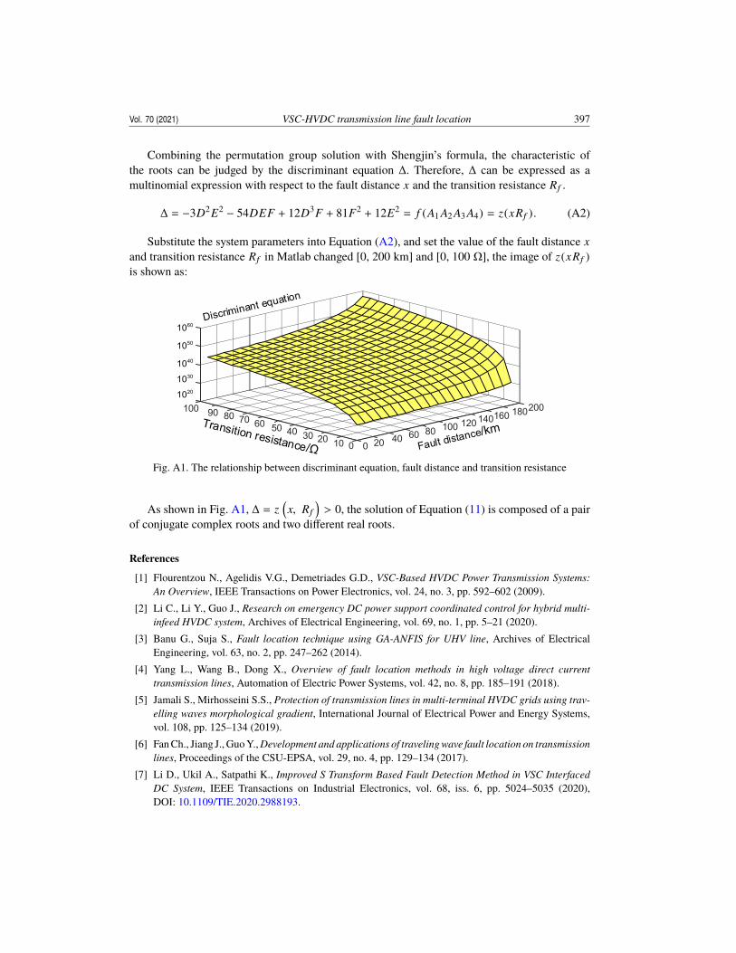
Combining the permutation group solution with Shengjin’s formula, the characteristic ofthe roots can be judged by the discriminant equation ∆. Therefore, ∆ can be expressed as amultinomial expression with respect to the fault distance x and the transition resistance Rf .

∆ = −3D2E2 − 54DEF + 12D3F + 81F2 + 12E2 = f (A1 A2 A3 A4) = z(xRf ). (A2)

Substitute the system parameters into Equation (A2), and set the value of the fault distance xand transition resistance Rf in Matlab changed [0, 200 km] and [0, 100 Ω], the image of z(xRf )is shown as:

100 20090 18080 16070 14060 12050 10040 8030 6020 4010 200 0

60105010401030102010

Fig. A1. The relationship between discriminant equation, fault distance and transition resistance

As shown in Fig. A1, ∆ = z(x, Rf

)> 0, the solution of Equation (11) is composed of a pair

of conjugate complex roots and two different real roots.

References

[1] Flourentzou N., Agelidis V.G., Demetriades G.D., VSC-Based HVDC Power Transmission Systems:An Overview, IEEE Transactions on Power Electronics, vol. 24, no. 3, pp. 592–602 (2009).

[2] Li C., Li Y., Guo J., Research on emergency DC power support coordinated control for hybrid multi-infeed HVDC system, Archives of Electrical Engineering, vol. 69, no. 1, pp. 5–21 (2020).

[3] Banu G., Suja S., Fault location technique using GA-ANFIS for UHV line, Archives of ElectricalEngineering, vol. 63, no. 2, pp. 247–262 (2014).

[4] Yang L., Wang B., Dong X., Overview of fault location methods in high voltage direct currenttransmission lines, Automation of Electric Power Systems, vol. 42, no. 8, pp. 185–191 (2018).

[5] Jamali S., Mirhosseini S.S., Protection of transmission lines in multi-terminal HVDC grids using trav-elling waves morphological gradient, International Journal of Electrical Power and Energy Systems,vol. 108, pp. 125–134 (2019).

[6] FanCh., Jiang J., GuoY.,Development and applications of traveling wave fault location on transmissionlines, Proceedings of the CSU-EPSA, vol. 29, no. 4, pp. 129–134 (2017).

[7] Li D., Ukil A., Satpathi K., Improved S Transform Based Fault Detection Method in VSC InterfacedDC System, IEEE Transactions on Industrial Electronics, vol. 68, iss. 6, pp. 5024–5035 (2020),DOI: 10.1109/TIE.2020.2988193.

https://doi.org/10.1109/TIE.2020.2988193


[8] Qin J., Peng L., Wang H., Single terminal methods of traveling wave fault location in transmission lineusing wavelet transform, Automation of Electric Power Systems, vol. 29, no. 19, pp. 62–65+86 (2005).

[9] Xu X., Sheng G., Liu Y., Fault location method for transmission lines based on distributed travelingwave detection, Proceedings of the Chinese Society of Universities for Electric Power System and itsAutomation, vol. 24, no. 3, pp. 134–138 (2012).

[10] He Z., Liao K., Li X., Lin S., Yang J., Mai R., Natural Frequency-Based Line Fault Location in HVDCLines, IEEE Transactions on Power Delivery, vol. 29, no. 2, pp. 851–859 (2014).

[11] He Z., Liao K., Natural frequency-based protection scheme for voltage source converter-based high-voltage direct current transmission lines, IETGeneration, Transmission andDistribution, vol. 9, no. 13,pp. 1519–1525 (2015).

[12] Cai X., Song G., Gao S., A novel fault-location method for VSC-HVDC transmission lines based onnatural frequency of current, Proceedings of the CSEE, vol. 31, no. 28, pp. 112–119 (2011).

[13] Zhang Y., Wang H., Li T., Combined single-end fault location method for LCC-VSC hybrid HVDCtransmission lines, Automation of Electric Power Systems, vol. 43, no. 21, pp. 187–199 (2019).

[14] Suonan J., Gao S., Song G., Jiao Z., Kang X., A Novel Fault-Location Method for HVDC TransmissionLines, IEEE Transactions on Power Delivery, vol. 25, no. 2, pp. 1203–1209 (2010).

[15] Yanxia Z., JianW., Huilan J., Fang Z., A Novel Fault Location Method for Hybrid-HVDC TransmissionLine, 2019 IEEE Power and Energy Society General Meeting (PESGM), Atlanta, GA, USA, pp. 1–5(2019).

[16] Song G., Zhou D., Jiao Z., A novel fault location principle for HVDC transmission lines, Automationof Electric Power Systems, vol. 31, no. 24, pp. 57–61 (2007).

[17] Kang L., Tang K., Luo J., Two-terminal fault location of monopolar earth fault in HVDC transmissionlines, Power System Technology, vol. 38, no. 8, pp. 2268–2273 (2014).

[18] Jin Y., Fletcher J.E., O’Reilly J., Short- circuit and ground fault analyses and location in VSC-based DCnetwork cables, IEEE Transactions on Industrial Electronics, vol. 59, no. 10, pp. 3827–3837 (2012).

[19] Liu D., Wei T., Huo Q., DC side line-to-line fault analysis of VSC-HVDC and DC-fault-clearingmethods, 2015 5-th International Conference on Electric Utility Deregulation and Restructuring andPower Technologies (DRPT), Changsha, China, pp. 2395–2399 (2015).

[20] Dessouky S.S., Fawzi M., Ibrahim H.A., Ibrahim N.F., DC Pole to Pole Short Circuit Fault Anal-ysis in VSC-HVDC Transmission System, 2018 Twentieth International Middle East Power SystemsConference (MEPCON), Cairo, Egypt, pp. 900–904 (2018).

[21] Ke J., Meng L.I., Shu B.T., A voltage resonance-based single-ended online fault location algorithm forDC distribution networks, Sciences China Technological Sciences, vol. 59, no. 5, pp. 721–729 (2016).

[22] Hwang K.S., Chang F.C., Chiou J.Y., A numerical approach to fast evaluation of time-invariant systemresponses, International Journal of Computer Mathematics, vol. 73, no. 3, pp. 361–369 (2000).

[23] Liu D., HuW., Chen Z., SVD-TLS extending Prony algorithm for extracting UWB radar target feature,Journal of Systems Engineering and Electronics, vol. 19, no. 2, pp. 286–291 (2008).

[24] XuM.M.,XiaoL.Y.,WangH.F.,A prony-based method of locating short-circuit fault in DC distributionsystem, 2-nd IETRenewable PowerGenerationConference (RPG2013), Beijing, China, pp. 1–4 (2013).

Documents

VSC-HVDC transmission line fault location based on