Embed Size (px)
Citation preview
eeh power systemslaboratory
David Lehnen
MATLAB Simulator for Dynamic Studies withVSC-HVDC Links
Semester ThesisPSL1308
EEH – Power Systems LaboratorySwiss Federal Institute of Technology (ETH) Zurich
Examiner: Prof. Dr. Göran AnderssonSupervisor: Markus Imhof
Zurich, July 5, 2013

AbstractIn the context of this semester project, an existing dynamic simulator was combinedwith an existing Optimal Power Flow (OPF) framework in a way, such that the startvalues for the dynamic simulation are set according to the OPF result. This approachsolves the problem that the initialization of the dynamic simulation sometimes doesnot converge, i.e. does not find the steady state start values for the simulation. Inaddition, the set points of the High Voltage Direct Current (HVDC) lines should bedetermined as well with the OPF result. This means that the power transfer throughthe HVDC line and the reactive power production at both ends of the HVDC line areset, such that the system is optimal, e.g. that there are minimal losses in the system.The OPF calculation can be executed with either flexible generation or with a givenproduction profile for the generators. In the second case, only the powers of the HVDClines are optimized, while in the first case the production of the generators is optimizedas well.In this thesis, the functions combining the dynamic simulator and the OPF frameworkare presented together with some functions which simplify the definition of plots.
KurzfassungIm Rahmen dieser Semesterarbeit wurde ein bereits vorhandener dynamischer Simu-lator mit einem bereits existierenden Optimalen-Lastfluss-Framework so kombiniert,dass die Startwerte für die dynamische Simulation entsprechend dem Resultat der op-timalen Lastflussberechnung gesetzt werden. Damit wurde das Problem gelöst, dassdie Initialisierung des dynamischen Simulators manchmal nicht konvergiert, d.h. diestatoionären Startwerte für die Simulation nicht gefunden werden können. Zusätzlichwerden auch die Sollwerte der Hochspannungs-Gleichstrom-Übertragungs-Leitungen(HGÜ) anhand des optimalen Lastflussergebnisses gesetzt. Das heisst, dass die Leis-tung über die HGÜ-Leitungen und die Blindleistungseinspeisung an beiden Enden derLeitung so eingestellt wird, dass das System optimal ist, z.B. die Verluste im Systemminimal sind. Die optimale Lastflussberechnung kann entweder mit variabler odervorgegebener Produktionsmenge der Generatoren ausgeführt werden. Im zweiten Fallwerden nur die Leistungen der HGÜ-Leitungen optimiert, während im ersten Fall zusät-zlich auch die Produktionsmenge der Generatoren optimiert wird.In dieser schriftlichen Arbeit werden die Funktionen vorgestellt, die den dynamischenSimulator mit dem Optimalen-Lastfluss-Framework auf diese Art kombinieren zusam-men mit weiteren Funktionen, die das Erstellen von Plots vereinfachen.
iii

eeh power systemslaboratory
EEH — Power Systems LaboratoryPhysikstrasse 3ETH Zentrum, ETL G.28CH-8092 Zurich
Markus ImhofPhone: +41 (0)44 632 [email protected]
psl1308
Semester Thesis FS 2013
assigned to David Lehnen ([email protected])
MATLAB Simulator for Dynamic Studies with VSC-HVDC Links
Abstract
Historically our transmission system was not designed for power trading, but for the exchangeof regulating power. As a result of the deregulation of power markets, particularly in Eu-rope, the tie-lines are quite often subject to heavy loading caused by power trading betweencountries. Deregulation also brings increased variations in power flows. These developmentsare the cause of severe challenges for the transmission system and its operators. Withoutadding more transport capacity and controllability to the grid could cause the instability ofthe transmission system. High Voltage Direct Current (HVDC) Voltage Source Converters(VSC) can be used to stabilize and control the AC transmission system. With HVDC-VSCactive and reactive power can be controlled independently on each converter station.
Task
This semester thesis aims to write a dynamic simulator in MATLAB. The simulator coredeveloped by Turhan Demiray will be used to develop a combined power flow and dynamic
1
simulation environment. The student has to familiarize himself with the di!erent simulatorenvironments and combine both environment to one. The student will write a report todocument his work. This work is also understood as documentation for the newly createdsimulation environment. Following features should be programmed:
• Power flow should be used as a initial value for the dynamic simulation
• Changes of the model should be tracked in the dynamic and the steady state systems
• Program hast to be modular, so that di!erent systems and models can be addedautomatically
• Data output routine
• User friendly interface
At the end the student will give a short presentation about his work and the results of hisstudies.The project outline will be as follows:
• Literature survey power flow and dynamic simulations as well as VSC-HVDC
• Familiarize with the steady state and the dynamic simulation environment
• Build new simulation environment in MATLAB
• Test the new simulation environment with di!erent test scenarios in the Europeansystem
• Write report & presentation
Requirements
This work requires knowledge of MATLAB, as well as the capability of working independently,analyzing the results and documenting the work. The students should also have a basicknowledge in power flow calculation and optimal power flow calculation.
References
[1] MATPOWER - A MATLAB Power System Simulation Packagehttp://www.pserc.cornell.edu/matpower/
[2] Prof. G. Andersson; Modelling and Analysis of Electrical Power Systems; Lecturenotes; 2010http://www.eeh.ee.ethz.ch/de/eeh/lehre/vorlesungen/viewcourse/227-0526-00.html
[3] T. Haase; Anforderungen an eine durch Erneuerbare Energien gepragten Energiev-ersorgung - Untersuchung des Regelverhaltens von Kraftwerken und Verbundnetzen;Ph.D. dissertation, Universitat Rostock, 2006
2
[4] P. Kundur, N. Balu, and M. Lauby; Power system stability and control ; McGraw-HillNew York, 1994
[5] T. Demiray; Simulation of Power System Dynamics using Dynamic Phasor Models;Ph.D. dissertation; ETH Zurich, 2008
Schedule
Start: 25. February 2013End: 10. June 2013Supervisor: Markus ImhofExaminer: Prof. Dr. Goran Andersson
Zurich, 21. February 2013
D. Lehnen M. Imhof
Prof. Dr. G. Andersson
3

Contents
Abstract iii
1. Introduction 5
2. Fundamentals 72.1. Optimal Power Flow . . . . . . . . . . . . . . . . . . . . . . . . . . . . 7
2.1.1. Network model . . . . . . . . . . . . . . . . . . . . . . . . . . . 82.1.2. HVDC model . . . . . . . . . . . . . . . . . . . . . . . . . . . . 9
2.2. Dynamic Simulation of Power Systems . . . . . . . . . . . . . . . . . . 11
3. Documentation/Manual of the Simulator 133.1. Transient Dynamic Simulator . . . . . . . . . . . . . . . . . . . . . . . 14
3.1.1. Dynamic System Data Format - tdsysformat . . . . . . . . . . 153.1.2. MPC Interface . . . . . . . . . . . . . . . . . . . . . . . . . . . 17
3.2. OPF . . . . . . . . . . . . . . . . . . . . . . . . . . . . . . . . . . . . . 183.2.1. OPF System Data Format - opfsysformat . . . . . . . . . . . . 18
3.3. Transformation of Dynamic System Data to OPF System Data . . . . . 193.4. Start Values and HVDC Set Points . . . . . . . . . . . . . . . . . . . . 203.5. Load System with Stored Start Values . . . . . . . . . . . . . . . . . . 223.6. Record and Plot Management . . . . . . . . . . . . . . . . . . . . . . . 22
3.6.1. Before Simulation . . . . . . . . . . . . . . . . . . . . . . . . . . 233.6.2. After Simulation . . . . . . . . . . . . . . . . . . . . . . . . . . 25
4. Results, Discussion and Outlook 274.1. Accuracy of Start Values . . . . . . . . . . . . . . . . . . . . . . . . . . 274.2. Initialization Performance with and without Start Values . . . . . . . . 274.3. Discussion . . . . . . . . . . . . . . . . . . . . . . . . . . . . . . . . . . 274.4. Outlook . . . . . . . . . . . . . . . . . . . . . . . . . . . . . . . . . . . 29
Bibliography 31
A. Naming Conventions 33
B. Simulation Parameters 37
C. Test System 39
D. Code Style Guidelines 47
ix

List of Abbreviations
AC Alternating CurrentAVR Automatic Voltage RegulatorDAEs Differential-Algebraic EquationsFACTS Flexible Alternating Current Transmission SystemHVDC High Voltage Direct CurrentHVDC-VSC High Voltage Direct Current Voltage Source ConverterMIPS Matlab Interior Point SolverMPC Model Predictive ControlOPF Optimal Power FlowPF Power FlowPSS Power System StabilizerTDS Transient Dynamic SimulatorVSC Voltage Source Converter
1


Preface
This work was created in the context of a semester thesis at the Power Systems Labora-tory of the ETH Zurich in the spring semester 2013. During this work I got an insighthow power systems can be simulated, both in steady state as well as dynamically andwhat difficulties thereby may arise.
At this point I would like to thank my supervisor Markus Imhof for the excellentsupport during this project.
3

1. Introduction
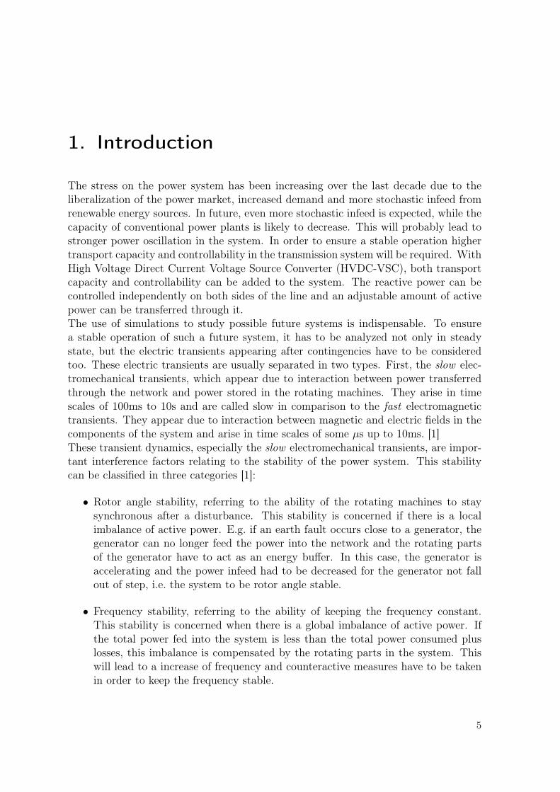
The stress on the power system has been increasing over the last decade due to theliberalization of the power market, increased demand and more stochastic infeed fromrenewable energy sources. In future, even more stochastic infeed is expected, while thecapacity of conventional power plants is likely to decrease. This will probably lead tostronger power oscillation in the system. In order to ensure a stable operation highertransport capacity and controllability in the transmission system will be required. WithHigh Voltage Direct Current Voltage Source Converter (HVDC-VSC), both transportcapacity and controllability can be added to the system. The reactive power can becontrolled independently on both sides of the line and an adjustable amount of activepower can be transferred through it.The use of simulations to study possible future systems is indispensable. To ensurea stable operation of such a future system, it has to be analyzed not only in steadystate, but the electric transients appearing after contingencies have to be consideredtoo. These electric transients are usually separated in two types. First, the slow elec-tromechanical transients, which appear due to interaction between power transferredthrough the network and power stored in the rotating machines. They arise in timescales of 100ms to 10s and are called slow in comparison to the fast electromagnetictransients. They appear due to interaction between magnetic and electric fields in thecomponents of the system and arise in time scales of some µs up to 10ms. [1]These transient dynamics, especially the slow electromechanical transients, are impor-tant interference factors relating to the stability of the power system. This stabilitycan be classified in three categories [1]:
• Rotor angle stability, referring to the ability of the rotating machines to staysynchronous after a disturbance. This stability is concerned if there is a localimbalance of active power. E.g. if an earth fault occurs close to a generator, thegenerator can no longer feed the power into the network and the rotating partsof the generator have to act as an energy buffer. In this case, the generator isaccelerating and the power infeed had to be decreased for the generator not fallout of step, i.e. the system to be rotor angle stable.
• Frequency stability, referring to the ability of keeping the frequency constant.This stability is concerned when there is a global imbalance of active power. Ifthe total power fed into the system is less than the total power consumed pluslosses, this imbalance is compensated by the rotating parts in the system. Thiswill lead to a increase of frequency and counteractive measures have to be takenin order to keep the frequency stable.
5
• Voltage stability, referring to the ability to keep all voltages in system constant.Since the voltage in the transmission system is highly coupled to reactive power,this stability is concerned when there is a imbalance of reactive power. The im-balance is usually only a local one, because reactive power cannot be transportedas well as reactive power in a transmission system where the reactance is muchhigher than the resistance.
To study the stability in a possible future system with HVDC lines, the transientdynamics have to be simulated. For this, the Transient Dynamic Simulator by T.Demiray can be used [3]. However, the initialization in this simulator is not often ableto find a solution when starting with a flat start, i.e. using the default values of themodels, especially all voltage magnitudes are set to 1 p.u., and all voltage angles to 0.Therefore the start values have to be set more closely to the solution. In order that oneis not obliged to tune the start values until the initialization converges, the motivationfor this project was to calculate the start values for the dynamic simulation with anOptimal Power Flow (OPF). In addition also the HVDC set points, i.e. the activepower transfer and the reactive power injected at both ends, is set optimally accordingto the OPF result.To do this, two functions have been implemented. First, a function which convertsthe system data for the dynamic simulator to system data useable by the OPF. Andsecond, a function which sets the start values and HVDC set points according to theOPF result.
This report is structured as following. In chapter 2, the mathematical basics of the OPFand of the dynamic simulation are discussed. Chapter 3 describes the implementationand usage of the functions. This part can be seen as a manual for the combinedsimulator. For a quick reference, the input and output arguments of the importantfunctions are described in boxes. Finally, in chapter 4, the initialization with andwithout set start values is compared and a short outlook is given.
6
2. Fundamentals
In this chapter the basics of both used simulators are discussed. Sec. 2.1 describes theOPF method and how High Voltage Direct Current (HVDC) lines are modeled in thiscontext and in Sec. 2.2 the basics of dynamic simulation of power systems are brieflydelineated.
2.1. Optimal Power Flow
OPF refers to methods which are determining how the set points in a systems shouldbe modified in order that the system has optimal performance without violating anylimits of the system. This can be formulated mathematically like this:
minx
f(x)
subject to g(x) = 0
h(x) ≤ 0
where x is the system state, i.e. the complex voltage V = Uejθ and apparent powerinjection Sinj = Pinj +jQinj in every node. f(x) is called objective function and specifieshow the optimum is defined. Usually one is interested in minimal costs for power pro-duction. In this case, the result of the OPF run is the cheapest allocation of generators,so that the resulting power flows do not violate any limits of a line or a transformer.Another common optimum is minimal losses in the system, which can be calculated bydefining the costs of all generators identically. How the different states depend on eachother is defined with the multidimensional function g(x), called equality constraints.It describes the physical boundary conditions in the system, such as the power balancein every node. The inequality constraints h(x), which is a multidimensional functionas well, specifies the physical limits in the system, e.g. the voltage limitations. [2, 6]
The following two subsections describe how the f(x), g(x) and h(x) functions aredefined for a network without and with HVDC lines.
7
2.1.1. Network model
In a system without HVDC lines the power injections are the produced active andreactive power by the generators. Hence the system state is in this case
x =
θUPgQg
.
Assuming one is interested in minimal costs for power generation, the objective functionf(x) is the sum of costs of all generators
f(x) =
Ngen∑i=1
fi(x) ,
where fi(x), the cost of generator i, is usually a polynomial of the form
fi(x) = c0 + c1Pgi + c2P2gi
+ . . . ,
typically up to the 2nd order.
These costs are in an OPF calculation minimized with respect to the equality con-straints g(x) and inequality constraints h(x) of the system. The equality constraintsg(x) are essentially the set of the apparent power balance equations for every node∑
m∈Ωk
(Pkm + jQkm) = Pinj,k + jQinj,k for k = 1, . . . , N ,
where N is the number of nodes in the network and Ωk is the set of all nodes adjacentto the node k. Pinj,k+jQinj,k is the power injection, i.e. the difference between producedand consumed power at node k. Furthermore, Pkm and Qkm are the active and reactivepower flow through the branch from node k to m and can be formulated with
Pkm = U2kgkm − UkUmgkm cos(θkm)− UkUmbkm sin(θkm) (2.1)
Qkm = −U2k (bkm + bshkm) + UkUmbkm cos(θkm)− UkUmgkm sin(θkm) , (2.2)
where Uk = |Vk|, θk = arg(Vk), θkm = θk − θm and gkm + jbkm = (Rkm + jXkm)−1 [1].
Finally, the inequality constraints h(x) assemble all upper and lower limits of the systemstate
xk,max + xk ≤ 0
−xk + xk,min ≤ 0 ,
for example the minimal and maximal voltage magnitude at each node
Uk,max + Uk ≤ 0
−Uk + Uk,min ≤ 0 .
8
But not only variables of the system state are physically limited. Other limits, e.g. thelimits of the branches, exists in the system as well and have to be described in h(x).To do this, the limited variable has to be described as a function of the system statex. For example power flow through a line Pik is limited, i.e. has to satisfy
Pik − Pi,max ≤ 0
−Pik + Pi,min ≤ 0 .
where Pik is expressed with formula (2.1) as a function of the system state.
2.1.2. HVDC model
A HVDC line in the network can be modeled with power injections at the nodeswhere the line is connected to the network, meaning that the active and reactive powerinjections at both link nodes are added to the system state
x =
θUPgQg
Pinj
Qinj
.
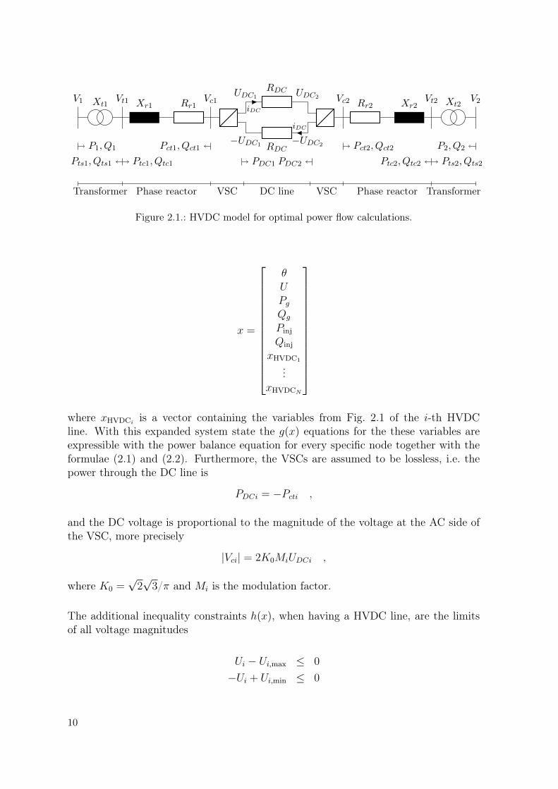
Since the active power infeed at one side of the line will reach the other end except forsome losses, the active power injections at both ends of the line depend on each otherand a model for this dependency has to be introduced. In addition, this model shouldfit well with the model used in the dynamic simulation, in order that the correct startvalues for the dynamic simulation can be exported later. The circuit diagram depictedin Fig. 2.1 is the steady state simplified model of the model used in the dynamicsimulation [4]. This model consists of four parts: The grid voltage at both sides is firsttransformed to a suitable voltage level for the Voltage Source Converter (VSC). Thenthe high switching harmonics coming from the VSC are filtered with a phase reactor.After that, the VSC inverts or rectifies the AC voltage to DC, before the power istransferred through the HVDC line. The power transfer takes place on the go as wellas on the return line.The complex voltages at the end nodes V1 and V2 as well as the power injectionsP1, P2, Q1, Q2 are linked to the network. All the other voltages and powers have to beexpressed with a series of g(x) functions. Actually, one g(x) function describing thedependency between both sides would be sufficient. But to define the g(x) functionsless complicated and to be able to export more start values later, the variables shownin Fig. 2.1 are added to the system state
9
Xt1 Xr1 Rr1V1 Vt1 Vc1
UDC1
−UDC1
RDC
iDC
RDC
iDC
UDC2
−UDC2
Rr2 Xr2 Xt2Vc2 Vt2 V2
P1, Q1
Ptc1, Qtc1Pts1, Qts1
Pct1, Qct1
PDC1 PDC2
Pct2, Qct2
Ptc2, Qtc2 Pts2, Qts2
P2, Q2
Transformer Phase reactor VSC DC line VSC Phase reactor Transformer
Figure 2.1.: HVDC model for optimal power flow calculations.
x =
θUPgQg
Pinj
Qinj
xHVDC1
...xHVDCN
where xHVDCi
is a vector containing the variables from Fig. 2.1 of the i-th HVDCline. With this expanded system state the g(x) equations for the these variables areexpressible with the power balance equation for every specific node together with theformulae (2.1) and (2.2). Furthermore, the VSCs are assumed to be lossless, i.e. thepower through the DC line is
PDCi = −Pcti ,
and the DC voltage is proportional to the magnitude of the voltage at the AC side ofthe VSC, more precisely
|Vci| = 2K0MiUDCi ,
where K0 =√
2√
3/π and Mi is the modulation factor.
The additional inequality constraints h(x), when having a HVDC line, are the limitsof all voltage magnitudes
Ui − Ui,max ≤ 0
−Ui + Ui,min ≤ 0
10
and active and reactive power limits of all flows
Pik − Pik,max ≤ 0
−Pik + Pik,min ≤ 0
Qik −Qik,max ≤ 0
−Qik +Qik,min ≤ 0 .
Since all variables shown in Fig. 2.1 are contained in the system state, the h(x) equa-tions are definably very convenient as well.
In principle there are no costs for a HVDC line, since the branches in the AC networkhave no cost either. But by introducing a negative cost function, e.g.
fHVDC(x) = c2(P1 + P2)2, with c2 < 0 (2.3)
one can force the system to transfer more power through the HVDC line.
The HVDC model described in this section is implemented in the file opfmdl_hvdc.-symdef.
2.2. Dynamic Simulation of Power Systems
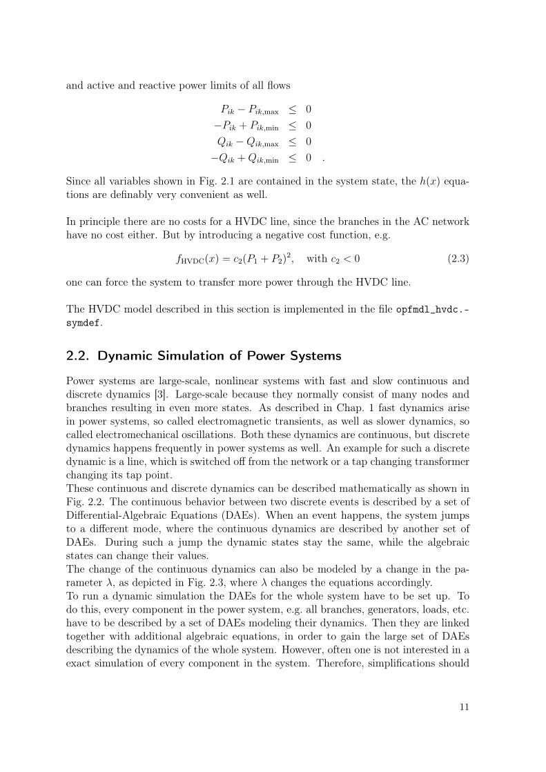
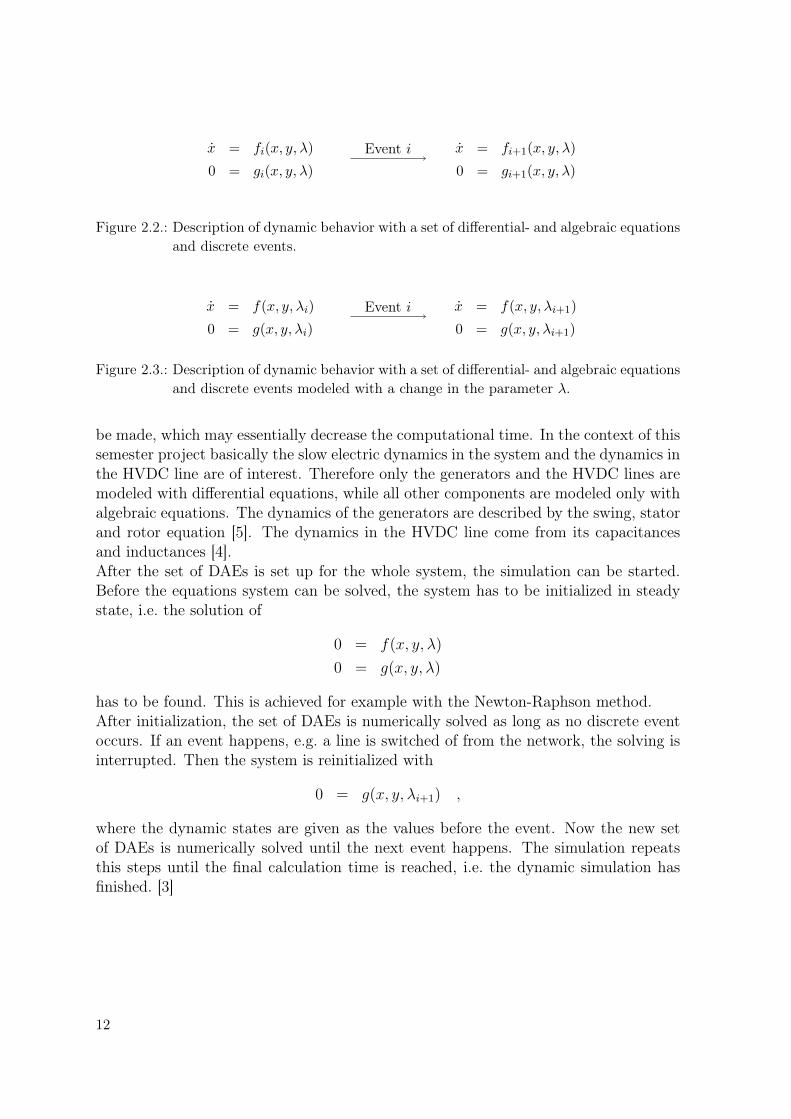
Power systems are large-scale, nonlinear systems with fast and slow continuous anddiscrete dynamics [3]. Large-scale because they normally consist of many nodes andbranches resulting in even more states. As described in Chap. 1 fast dynamics arisein power systems, so called electromagnetic transients, as well as slower dynamics, socalled electromechanical oscillations. Both these dynamics are continuous, but discretedynamics happens frequently in power systems as well. An example for such a discretedynamic is a line, which is switched off from the network or a tap changing transformerchanging its tap point.These continuous and discrete dynamics can be described mathematically as shown inFig. 2.2. The continuous behavior between two discrete events is described by a set ofDifferential-Algebraic Equations (DAEs). When an event happens, the system jumpsto a different mode, where the continuous dynamics are described by another set ofDAEs. During such a jump the dynamic states stay the same, while the algebraicstates can change their values.The change of the continuous dynamics can also be modeled by a change in the pa-rameter λ, as depicted in Fig. 2.3, where λ changes the equations accordingly.To run a dynamic simulation the DAEs for the whole system have to be set up. Todo this, every component in the power system, e.g. all branches, generators, loads, etc.have to be described by a set of DAEs modeling their dynamics. Then they are linkedtogether with additional algebraic equations, in order to gain the large set of DAEsdescribing the dynamics of the whole system. However, often one is not interested in aexact simulation of every component in the system. Therefore, simplifications should
11
Event ix = fi(x, y, λ)
0 = gi(x, y, λ)
x = fi+1(x, y, λ)
0 = gi+1(x, y, λ)
Figure 2.2.: Description of dynamic behavior with a set of differential- and algebraic equationsand discrete events.
Event ix = f(x, y, λi)
0 = g(x, y, λi)
x = f(x, y, λi+1)
0 = g(x, y, λi+1)
Figure 2.3.: Description of dynamic behavior with a set of differential- and algebraic equationsand discrete events modeled with a change in the parameter λ.
be made, which may essentially decrease the computational time. In the context of thissemester project basically the slow electric dynamics in the system and the dynamics inthe HVDC line are of interest. Therefore only the generators and the HVDC lines aremodeled with differential equations, while all other components are modeled only withalgebraic equations. The dynamics of the generators are described by the swing, statorand rotor equation [5]. The dynamics in the HVDC line come from its capacitancesand inductances [4].After the set of DAEs is set up for the whole system, the simulation can be started.Before the equations system can be solved, the system has to be initialized in steadystate, i.e. the solution of
0 = f(x, y, λ)
0 = g(x, y, λ)
has to be found. This is achieved for example with the Newton-Raphson method.After initialization, the set of DAEs is numerically solved as long as no discrete eventoccurs. If an event happens, e.g. a line is switched of from the network, the solving isinterrupted. Then the system is reinitialized with
0 = g(x, y, λi+1) ,
where the dynamic states are given as the values before the event. Now the new setof DAEs is numerically solved until the next event happens. The simulation repeatsthis steps until the final calculation time is reached, i.e. the dynamic simulation hasfinished. [3]
12
3. Documentation/Manual of theSimulator
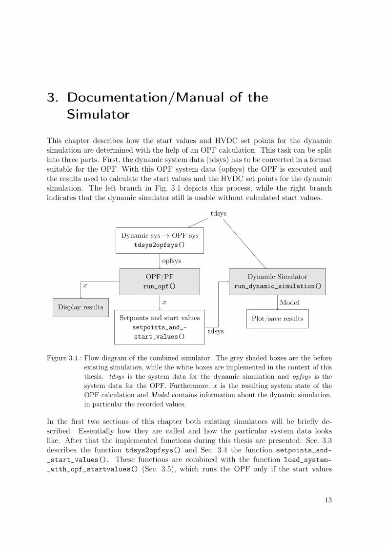
This chapter describes how the start values and HVDC set points for the dynamicsimulation are determined with the help of an OPF calculation. This task can be splitinto three parts. First, the dynamic system data (tdsys) has to be converted in a formatsuitable for the OPF. With this OPF system data (opfsys) the OPF is executed andthe results used to calculate the start values and the HVDC set points for the dynamicsimulation. The left branch in Fig. 3.1 depicts this process, while the right branchindicates that the dynamic simulator still is usable without calculated start values.
OPF/PFrun_opf()
Dynamic Simulatorrun_dynamic_simulation()
Dynamic sys → OPF systdsys2opfsys()
Setpoints and start valuessetpoints_and_-start_values()
tdsys
Display results
Plot/save results
opfsys
x
x
Model
tdsys
Figure 3.1.: Flow diagram of the combined simulator. The grey shaded boxes are the beforeexisting simulators, while the white boxes are implemented in the context of thisthesis. tdsys is the system data for the dynamic simulation and opfsys is thesystem data for the OPF. Furthermore, x is the resulting system state of theOPF calculation and Model contains information about the dynamic simulation,in particular the recorded values.
In the first two sections of this chapter both existing simulators will be briefly de-scribed. Essentially how they are called and how the particular system data lookslike. After that the implemented functions during this thesis are presented: Sec. 3.3describes the function tdsys2opfsys() and Sec. 3.4 the function setpoints_and-_start_values(). These functions are combined with the function load_system-_with_opf_startvalues() (Sec. 3.5), which runs the OPF only if the start values
13
are not already calculated and stored before. Finally in Sec. 3.6 some functions arepresented, which handle the record and plot management. This is important, since itis not possible to record all states during the dynamic simulation.
3.1. Transient Dynamic Simulator
The used dynamic simulator was implemented by T. Demiray in the context of hisPhD thesis Simulation of Power System Dynamics using Dynamic Phasor Models [3].This simulator, called Transient Dynamic Simulator, allows a very flexible definition ofthe system and its components. But because the core is used in the commercial toolNEPLAN, the source code is protected and only accessible with Matlab p-functions.Therefore the use of the dynamic simulator is only briefly explained on the basis ofthe input and output arguments of the function run_dynamic_simulation(), whichhandles all the p-function calls internally. It has the following input and output argu-ments:
Model = run_dynamic_simulation(tfinal, Components, Branches,Buselements, ExternalConnectionsWithnames, Disturbances,
RecordVars, Tdsparam, Mpcparam)
Input arguments:
tfinal : Simulation time in seconds.
[Components,Branches,Buselements,ExternalConnectionsWithnames] :System description in the tdssysformat. See Sec. 3.1.1.
Disturbances : A cell array of dimension N × 4, where N is the number ofparameter changes. Disturbances has the form:
time ’componentName’ ’parameterName’ newParamValue
it defines that at simulation time time the parameter parameterName of thecomponent componentName changes its value to newParamValue.
RecordVars : A cell array of dimension N × 2 specifying all states which shouldbe recorded during the simulation. Each row has to be in the form of
’comp1’ ’comp2’ ... ’compM’ ’var1’ ’var2’ ... ’varN’
which defines that for every component named comp1, comp2, . . ., compM allthe variables named var1, var2, . . ., varN will be recorded.
Tdsparam : A struct containing simulation parameters, such as for example inte-gration type, tolerance, and others. See App. B.
14
Mpcparam : A struct defining MPC parameters. See Sec. 3.1.2.
Output arguments:
Model : A struct containing information about the model. The field resultscontains the values of the variables specified by RecordVars for all time steps.
3.1.1. Dynamic System Data Format - tdsysformat
The dynamic system description has to define the set of differential- and algebraicequations
x = f(x, y, λi)
0 = g(x, y, λi) ,
describing the dynamics of the system (see Sec. 2.2). This is done in the TransientDynamic Simulator with the four cell Arrays Components, Branches, Buselements andExternalConnectionsWithnames. While Components describes the set of differential-and algebraic equations of each component, the three other cell arrays provide differentways to define the links between the components. The cell arrays are of the followingstructure:
Components: A cell array of dimension N×5, where N is the number of components inthe system. Each row corresponds to a component and has the following format:
’modelName’ [dynstates] [algstates] [param] ’componentName’
modelName a string specifying the model function and has to follow the namingconventions of Tab. A.1, in order that the conversion of the dynamic systemdata to the OPF system data works. The model function is a .m file, which isautomatically generated from the corresponding .symdef file. This automaticgeneration is done by calling
tda_create_symbolically_normal(’modelName.symdef’) ,
where it is necessary that the current working path is in the Models directory.The .symdef file defines the differential- and algebraic equations of the compo-nent and the names of the dynamic- and algebraic states as well as the namesof the parameters. A model of a specific component has to contain parameterswith the names defined in Tab. A.2. How a .symdef file is built can be found inSimulation of Power System Dynamics using Dynamic Phasor Models [3]. Fur-thermore, there are dynstates and algstates vectors setting the start valuesfor the first initialization run. parameters is a vector defining the parameters ofthe component and componentName is a string giving the component an uniquename.
15
Branches: A cell array of dimension N × 3, where N is the number of branches in thesystem. Each row corresponds to a branch and has the format:
’branchName’ ’bus1Name’ ’bus2Name’
branchName is a string defining the name of the branch component and bus1Nameand bus2Name are strings with the names of the nodes where the branch is con-nected to the network. Hence all elements of Branches have to refer to an uniquename in the 5th column of Components. With Branches the complex voltage atboth sides of the branch are linked with the complex voltage of the respectivenodes. This is done by linking the following variables with algebraic equations:
VD1branch = VDbus1 VD2branch = VDbus2
VQ1branch = VQbus1 VQ2branch = VQbus2
Thus the branch model has to have algebraic states with above names. Addition-ally, also the complex currents on both sides are required, i.e. ID1, IQ1, ID2 andIQ2, because they are balanced with Kirchhoff’s current law in every node.
Buselements: A cell array of dimension N×5, where N is the total number of genera-tors, loads and shunts in the system. Each row corresponds to such a buselementand has the format:
’buselementName’ ’nodeName’ ’avrName’ ’pssName’ ’govName’
buselementName is a string defining the name of the buselement connected tothe node specified with the string nodeName. If the buselement is a generator itscontrollers can be specified with avrName, pssName and govName. All elementsof Buselements have to refer to unique names in the 5th column of Components.The buselement is linked to the other components of the cell array with algebraicequations as following:
VDbuselement = VDbus
VQbuselement = VQbus
VTbuselement = VTAVR
EFDbuselement = EFDAVR
Qbuselement = QAVR
Wbuselement = WPSS
Pbuselement = Pgov
Wbuselement = Wgov
VQbuselement = VQgov
TMbuselement = TMgov
16
And the link between the AVR and PSS.
VPSSAVR = VPSSPSS
Thus every component model needs to have algebraic states with above mentionednames. Additionally, also the complex currents are required, i.e. IDbuselement,IQbuselement, because they are balanced with Kirchhoff’s current law in every node.
ExternalConnectionsWithnames: A cell array of dimension N × 4, where N is thenumber of additional customized connections in the system. Each row correspondsto such a connection and is of the format:
’component1Name’ ’var1Name’ ’component2Name’ ’var2Name’ ,
where all entries are strings specifying that the variable var1Name of the compo-nent component1Name is equal the variable var2Name of the component compo-nent2Name. Both component names have to refer to an unique name in the 5th
column of Components.
3.1.2. MPC Interface
In the Transient Dynamic Simulator it is possible to periodically execute an user-definedfunction by adding a component of the model tdm_block_sample_system. Hence thefollowing line is add to Components
’tdm_block_sample_system’ [] [] [param] ’sampleCompName’ ,
where sampleCompName is the unique name of the component and param is a structwith the two fields funcname and sampletime. This component causes an event afterevery time step sampletime where the function funcname is executed.This possibility can be used for example to modify the set points of the HVDC controllerwith Model Predictive Control (MPC). In order to define parameters for the executingfunction, the struct Mpcparam can be used. This input argument of run_dynamic-_simulation() is added as field in the Model struct.The struct Mpcparam needs thefields ControllerStates and ControllerOutput which defines the controller statesand the controller output variables in the format
’comp1’ ’comp2’ ... ’compM’ ’var1’ ’var2’ ... ’varN’ .
When initializing, these two cell arrays are used to construct the fields stateIdxand outputIdx, which are cell arrays for an easy access of the variables defined inControllerStates and ControllerOutput. For every variable defined in Controller-States there is a matrix in stateIdx of the form
[modelIdx, varIdx] ,
indicating that the varIdx-th variable in the modelIdx-th model is a controller state.outputIdx has the same matrices for the variables defined in ControllerOutput.
17
3.2. OPF
The Optimal Power Flow (OPF) core was implemented by T. Demiray as well, al-though the optimization itself is done with Matpower’s Matlab Interior PointSolver (MIPS), which is a general nonlinear optimization solver [8]. The OPF coreby T. Demiray essentially calculates the input arguments for this MIPS function in anefficient way.The function run_opf() is executing the OPF and has the following input and outputarguments:
[x, Model, isConverged] = run_opf(Casestruct, Hvdc, Opfparam)
Input arguments:
Casestruct : A Matpower case struct. See Matpower manual [8].
Hvdc : Struct defining information about the HVDC lines with the following twofields:
Branches : A N × 2 matrix defining the nodes where the N HVDC lines isconnected to the network.
Components : A cell array of dimension n× 4 describing the model for eachHVDC line in the format
’modelName’ [startstates] [parameters] ’componentName’
Opfparam : : A struct defining settings for the OPF.
isPF : Boolean variable, defining if the generators have fixed (1-default) orflexible (0) production.
opt : A struct defining the options for the Matpower MIPS function. SeeMatpower maual [8].
Output arguments:
x : Vector containing the system state.
OpfModel : A struct containing information about the model.
isConverged : A boolean variable denoting if the OPF has converged or not.
3.2.1. OPF System Data Format - opfsysformat
The system data for the OPF consists of two parts. First, a Matpower case struct[7] defines the network and second, a struct Hvdc describs the HVDC lines with the
18
following two fields:
Branches : is a matrix of dimension N × 2 defining the nodes where the N HVDClines are connected to the network.
Components : is a cell array of dimension N ×4 describing the model for each HVDCline in the format
’modelName’ [startstates] [parameters] ’componentName’
where modelName specifies the model function automatically generated from a.symdef file. This file defines the objective function f(x), equality constraintsg(x) and inequality constraints h(x) of the model. The HVDC model describedin Sec. 2.1.2 is implemented with the model opfmdl_hvdc.symdef and accord-ingly with its automatically generated function opfmdl_hvdc.m. This function isgenerated by calling
opf_create_symbolically_normal(’modleName.symdef’) .
startstates a vector with the start values of the states and parameters a vectorwith the values of the parameters defined in the .symdef file. componentName isa string which gives the i-th HVDC line an unique name.
3.3. Transformation of Dynamic System Data to OPF SystemData
The function tdsys2opfsys() converts a dynamic system description (tdsysformat)into an OPF system description (opfssysformat). It has the following input and outputarguments:
[Casestruct, Hvdc] = tdsys2opfsys(Components, Branches, ...Buselements, opfsysFilename)
Input arguments:
[Components,Branches,Buselements] : System description in the tdssysformat.See section 3.1.1.
opfsysFilename (optional): A string defining the name of the file to store thesystem in the opfsysformat in the folder Systems. If it is an empty string thesystem is not saved.
Output arguments:
[Casestruct, Hvdc] : System description in the opfsysformat. See Sec. 3.2.1.
19
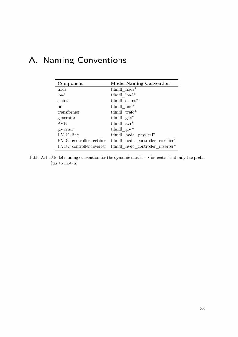
The function builds up the Matpower casestruct and the HVDC struct with the in-formation of the four cell arrays in the dynamic system description. To do this, thefunction determines first how many nodes, branches and generators are in the systemand creates empty matrices for the Matpower casestruct. To identify of which typea component is, it searches in the first row of Components, i.e. in the model names, fora component type specific prefix. In Tab. A.1 the naming conventions for the modelnames are shown. This prefixes are a necessary requirement that the function works.Now the empty Matpower casestruct fields have to be filled. This is achieved bysearching step by step all entries in the parameters vectors of Components and con-verting them accordingly. For this search the subfunction
paramValue = param_value(Param, modelPrefix, Components)
is repeatedly used. It returns a M ×N matrix called paramValue with the parametervalues of all M components, who have a model name starting with modelPrefix. TheN parameters are specified by the cell array of strings Param.After the Matpower casestruct is completed, the function saves it with Matpower’ssavecase() function in the Systems folder. To identify where the main folder is, thefunction get_main_folder_path(), which returns the absolute path to the main folder,is used.Now the function yet have to build up both fields of the Hvdc struct. While for thematrix Branches only the bus IDs have to be reconstructed from the node names,the parameters for the cell array Components are searched again with param_value().After this is done, the Hvdc struct is saved in the same file as the Matpower casestructand both structs are returned for a possible subsequent use.
3.4. Start Values and HVDC Set Points
The function setpoints_and_start_values() determines the start values and the setpoints of the HVDC controllers for the dynamic simulation based on the OPF result.It has the following input and output arguments:
Components = setpoints_and_start_values(x, OpfModel, ...Components, Branches)
Input arguments:
x : A vector of the optimal system state.
OpfModel : A struct containing information about the model.
[Components, Branches] : Cell arrays in the tdssysformat. See Sec. 3.1.1.
Output arguments:
Components : A cell array with start values and and adapted set points in thetdssysformat. See Sec. 3.1.1.
20
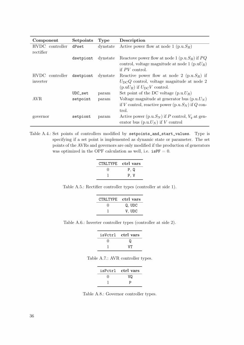
First, the function sets the start values of the algebraic states showed in Tab. A.3. Forother algebraic states, which are not contained in this table, the default start valuesas specified in the .symdef files, are taken. Secondly, the function determines the setpoints showed in Tab. A.4 and sets the parameters and dynamic states accordingly.Some set points, e.g. the active power through the HVDC line are implemented asdynamic states, so that they can be modified during the simulation. If the produc-tion of the generators has been optimized in the OPF calculation as well, i.e. a realOPF run was made, the set points of the governors and AVRs have to be modified, too.
This setting of start values and set points is achieved with following steps:
1. Constructing indices vector for an easy access the different parts of the OPF resultvector
x =
θUPgQg
PinjQinj
xHVDC1
...xHVDCN
.
2. Transformaton of the bus voltage into dq-coordinates and calculation of the powerflow and currents in every branch.
3. Determining the algebraic start vector for every component. This is done bycalling the subfunction
y0 = start_algstates(modelName, AlgStates),
for every component. AlgStates is a cell array with two columns, where the firstcolumn contains the names of the algebraic states and the second column thecorresponding start values. The function takes then the default algebraic statevector of the the model modelName and overwrites the states with the valuesspecified in AlgStates. If an algebraic state of AlgStates is not in the model,the default value as specified in the .symdef file is used.
4. Determining the dynamic start vector with the set points for the HVDC con-trollers. This is done with the subfunction
x0 = start_dynstates(modelName, DynStates),
which works similar to the function start_algstates().
5. Modify the parameters by changing the value in the parameter vector of Compon-ents. If the generators had fixed production in the OPF calculation, only the setpoint for UDC in the inverter is changed, otherwise the set points for the governorand the AVR are changed as well.
21
3.5. Load System with Stored Start Values
In order not to calculate the same set points and start values every time, the functionload_system_with_opf_startvalues() exists. It checks, wether there are alreadystored start values in the folder
Systems/OPF_startvalues ,
which are not older than the last modification time of the dynamic system data file. Ifthere are stored start values, the function loads and returns them. Otherwise, it runsan OPF and stores the found values. The function has following input and outputarguments:
[Components, Branches, Buselements, ExternalConnectionsWithnames, x,OpfModel] = load_system_with_opf_startvalues(tdsysFilename,
Opfparam)
Input arguments:
tdsysFilename : A string defining the name of the file to store the system in thetdsysformat in the folder Systems.
Opfparam : A struct defining the settings for the OPF.
isPF : A boolean variable, defining if the generators have fixed (1:default) orflexible (0) production.
opt : A struct defining the options for the Matpower MIPS function. SeeMatpower maual [8].
Output arguments:
[Components,Branches,Buselements,ExternalConnectionsWithnames] :System description in the tdssysformat. See Sec. 3.1.1.
x : A vector of the optimal system state.
OpfModel : A struct containing information about the model.
3.6. Record and Plot Management
Since a typical power system has a huge number of states, it would require a lot ofmemory to store them all at every time step of the simulation. Therefore it is moreproductive to define before the simulation which states are recorded. To do this thereare several functions in the folder Engine/Plots which allow to define these variablesefficiently. Note that variables in this context is a general term for both dynamic and
22
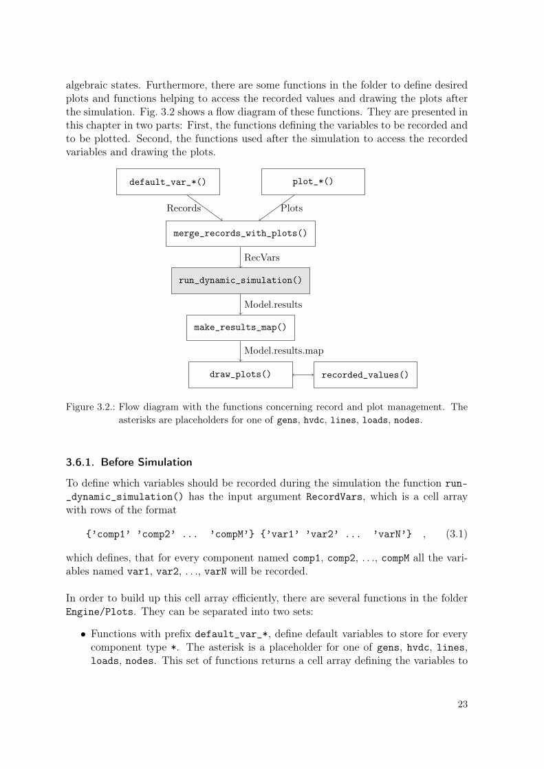
algebraic states. Furthermore, there are some functions in the folder to define desiredplots and functions helping to access the recorded values and drawing the plots afterthe simulation. Fig. 3.2 shows a flow diagram of these functions. They are presented inthis chapter in two parts: First, the functions defining the variables to be recorded andto be plotted. Second, the functions used after the simulation to access the recordedvariables and drawing the plots.
merge_records_with_plots()
default_var_*() plot_*()
run_dynamic_simulation()
make_results_map()
draw_plots() recorded_values()
Records Plots
RecVars
Model.results
Model.results.map
Figure 3.2.: Flow diagram with the functions concerning record and plot management. Theasterisks are placeholders for one of gens, hvdc, lines, loads, nodes.
3.6.1. Before Simulation
To define which variables should be recorded during the simulation the function run-_dynamic_simulation() has the input argument RecordVars, which is a cell arraywith rows of the format
’comp1’ ’comp2’ ... ’compM’ ’var1’ ’var2’ ... ’varN’ , (3.1)
which defines, that for every component named comp1, comp2, . . ., compM all the vari-ables named var1, var2, . . ., varN will be recorded.
In order to build up this cell array efficiently, there are several functions in the folderEngine/Plots. They can be separated into two sets:
• Functions with prefix default_var_*, define default variables to store for everycomponent type *. The asterisk is a placeholder for one of gens, hvdc, lines,loads, nodes. This set of functions returns a cell array defining the variables to
23
be recorded of the format (3.1). comp1, . . ., compM are the unique names of allcomponents of a specific type in the system. To detect all components the cellarray Components is an input argument of these functions.
• Functions with prefix plot_*, define a default plot for a component comp ofcomponent type *. To be able to plot after the simulation, the function definesthe variables to plot var1, var2, . . ., varN as variables to be recorded and returnsa cell array of the format
’comp’ ’var1’ ’var2’ ... ’varN’ ’functionName’ .
functionName is the name of the plot_* function itself, which is used after thesimulation by the function draw_plots() to call the function again and make theplots. Hence the same function has to do different things, depending if it is calledbefore or after the simulation. This distinction is achieved with the number ofinput arguments. If the function is called with only one input argument comp, i.e.the name of the component, the function returns a cell array as defined above. Ifthe function is called with an additional second input argument Model, containingamong other things the recorded values, the function will plot.A special case is the function plot_variable(), which plots one or more arbi-trary variables of a given component. In this function, additional to the name ofthe component comp the variables to plot varNames are specified with an inputargument as well. varNames can either be a string with the name of a variable ora cell array of strings with the names of the variables to plot. The distinction ifthe function should plot or return a cell array is achieved in this function throughthe presence of two or three input arguments.
A possible use of these functions looks as following:
Records = [ ...default_var_lines(Components);default_var_nodes(Components);default_var_gens(Components);];
Plots = [ ...plot_line('Line−01−02');plot_line('Line−02−03');plot_variable('Gen−01','P','Q');];
To combine the cell arrays Records and Plots to RecVars, the input argument for thedynamic simulation, the function
RecVars = merge_records_with_plots(Records, Plots, Components)
can be used, which in addition eliminates redundant defined variables, i.e. variableswhich are defined more than one time in Plots and/or Records.
24
3.6.2. After Simulation
After the dynamic simulation has terminated, it returns the recorded values with thestruct Model.results in two matrices. The matrix Model.results.x contains therecorded dynamic states and Model.results.y contains the recorded algebraic states.Each line in these matrices contains the values of a variable for every time step specifiedby the vector Model.results.time. To have an easy access to the stored variables thefunction
Map = make_resultsmap(Model)
constructs a map to identify in which matrix and in which line the stored values for avariable can be found. Map is a cell array where every line has the format:
’compName’ ’var1’, ..., ’varN’[
var1Idx ... varNIdxisAlgstate ... isAlgstate
]This map allows to find the recorded values of the variable varN of the componentcompName as following: By searching compName in the first column of Map we get theline of Map corresponding to the specific component. Then by searching at which indexthe variable varN is in the cell array in the second column of this line we get thecolumn of the matrix in the third column of this line at which we can find varNIdxand isAlgstate. The boolean variable isAlgstate indicates if the stored values ofthis variable are in Model.results.y, i.e. if isAlgstate = 1, or in Model.results.xotherwise. varNIdx specifies the line containing the recorded values in the respectivematrix. These steps are essentially what is done by the function
recVars = recorded_values(compName, varName, results) ,
where recVars are the recorded values of the variable varName of the componentcompName. In order that the function works, results has, besides the matrices x andy, also to contain the field map, generated by make_resultsmap().
The function recorded_values() is also used indirectly by the function
draw_plots(Model, Plots) ,
which draws the plots specified before the simulation. draw_plots() calls successivelyall the functions in the third column of Plots, with the additional argument Model,so that the plot_* functions are in the plot mode.
25

4. Results, Discussion and Outlook
In this chapter the accuracy of the set start values is studied and the initializationperformance with start values compared to the initialization performance using a flatstart. After this, these results are discussed and a short outlook for possible futureextension is given.
4.1. Accuracy of Start Values
The start values for the initialization run of the dynamic simulation are set very ac-curate with the OPF calculation. This can be tested with the the function compare-_start_values(). It compares the start values set by setpoints_and_start_values()with the values after the initialization run. If the deviation is larger than a specifictolerance the function throws an error. For the Two Area System described in App. C,the largest relative deviation is smaller than 10−6.
4.2. Initialization Performance with and without Start Values
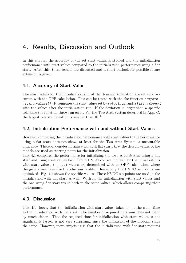
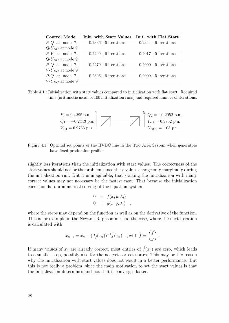
However, comparing the initialization performance with start values to the performanceusing a flat start does not show, at least for the Two Area System, a measurabledifference. Thereby, denotes initialization with flat start, that the default values of themodels are used as starting point for the initialization.Tab. 4.1 compares the performance for initializing the Two Area System using a flatstart and using start values for different HVDC control modes. For the initializationswith start values, the start values are determined with an OPF calculation, wherethe generators have fixed production profile. Hence only the HVDC set points areoptimized. Fig. 4.1 shows the specific values. These HVDC set points are used in theinitialization with flat start as well. With it, the initialization with start values andthe one using flat start result both in the same values, which allows comparing theirperformance.
4.3. Discussion
Tab. 4.1 shows, that the initialization with start values takes about the same timeas the initialization with flat start. The number of required iterations does not differby much either. That the required time for initialization with start values is notsignificantly faster, is not very surprising, since the dimension of the problem staysthe same. However, more surprising is that the initialization with flat start requires
27
Control Mode Init. with Start Values Init. with Flat StartP -Q at node 7,Q-UDC at node 9
0.2336s, 6 iterations 0.2344s, 6 iterations
P -V at node 7,Q-UDC at node 9
0.2299s, 6 iterations 0.2017s, 5 iterations
P -Q at node 7,V -UDC at node 9
0.2279s, 6 iterations 0.2000s, 5 iterations
P -Q at node 7,V -UDC at node 9
0.2306s, 6 iterations 0.2009s, 5 iterations
Table 4.1.: Initialization with start values compared to initialization with flat start. Requiredtime (arithmetic mean of 100 initialization runs) and required number of iterations.
7 9P1 = 0.4288 p.u.
Q1 = −0.2443 p.u.
Vm1 = 0.9733 p.u.
Q2 = −0.2052 p.u.
Vm2 = 0.9852 p.u.
UDC2 = 1.05 p.u.
Figure 4.1.: Optimal set points of the HVDC line in the Two Area System when generatorshave fixed production profile.
slightly less iterations than the initialization with start values. The correctness of thestart values should not be the problem, since these values change only marginally duringthe initialization run. But it is imaginable, that starting the initialization with manycorrect values may not necessary be the fastest case. That because the initializationcorresponds to a numerical solving of the equation system
0 = f(x, y, λi)
0 = g(x, y, λi) ,
where the steps may depend on the function as well as on the derivative of the function.This is for example in the Newton-Raphson method the case, where the next iterationis calculated with
xn+1 = xn − (Jf (xn))−1f(xn) ,with f =
(fg
).
If many values of x0 are already correct, most entries of f(x0) are zero, which leadsto a smaller step, possibly also for the not yet correct states. This may be the reasonwhy the initialization with start values does not result in a better performance. Butthis is not really a problem, since the main motivation to set the start values is thatthe initialization determines and not that it converges faster.
28
4.4. Outlook
The implemented functions during this project combine the before existing dynamicsimulator and OPF framework in a modular way. With them it is possible to determinethe start values for the dynamic simulation with an OPF calculation for an arbitrarysystem. This calculation is either possible as a real OPF or as an OPF, where thepower generation is given and not optimized. However, it is imaginable, that one isinterested in the start values with fixed HVDC set points. So far, this case is notautomatically calculable, but adding this possibility should not be too complex. Forexample one could simply fix the power injections in the OPF as the power generationis fixed in the second case above. The upper and lower limits of the power injectionsare set as equal. In this case nothing would be optimized anymore and instead of usingan OPF calculation a Power Flow (PF) calculation should be used. To do this, theHVDC lines could be included in the Matpower casestruct by modeling each HVDCline as additional two generators at the nodes, where the line is connected to the net-work. Another interesting and more challenging expansion to calculate the HVDC setpoints would be with a security constrained OPF or with another method consideringcontingencies.Since the Transient Dynamic Simulator allows a very flexible definition of additionalmodels, it is easily possible to add models. On the one hand models for componentswhich are not implemented yet, e.g. a model for FACTS devices or tap changing trans-formers could be added. On the other hand additional models for components, forwhich already exist a model, could be added to the model library or the existing mod-els be improved. Such an improvement could be the use of discrete states and statereset equations, which are supported by the Transient Dynamic Simulator as well [3].The state equations define how the discrete states change in case of an event and arenot yet used in the existing models.In any case, since HVDC lines are likely to play an important role in the power systemof the future it is worth simulating them in detail.
29

Bibliography
[1] Göran Andersson. Power System Analysis, Lecture notes. 2012.
[2] R. Bacher. SmartGrids: Optimization of Liberalized Electric Power Systems, Lec-ture Script. 2013.
[3] Turhan Demiray. Simulation of Power System Dynamics using Dynamic PhasorModels. PhD thesis, ETH Zürich, 2008.
[4] Markus Imhof and Göran Andersson. Dynamic modeling of vsc-hvdc converter.48th Int. Universities Power Engineering Conference, 2013.
[5] P. Kundur, N.Balu, and M Lauby. Power System Stability and Control. McGraw-Hill, New York, 1994.
[6] Marek Zima and Marija Bockarjova. Operation, Monitoring and Control Technologyof Power Systems, Lecture notes. 2013.
[7] R. D. Zimmerman, C. E. Murillo-Sánchez, and R. J. Thomas. MATPOWER:Steady-State Operations, Planning, and Analysis Tools for Power Systems Researchand Education. IEEE Trans. Power Syst., 26(1):12–19, February 2011.
[8] Ray D. Zimmerman and Carlos E. Murillo-Sanchez. Matpower 4.1 User’s Manual,12 2011.
31

A. Naming Conventions
Component Model Naming Conventionnode tdmdl_node*load tdmdl_load*shunt tdmdl_shunt*line tdmdl_line*transformer tdmdl_trafo*generator tdmdl_gen*AVR tdmdl_avr*governor tdmdl_gov*HVDC line tdmdl_hvdc_physical*HVDC controller rectifier tdmdl_hvdc_controller_rectifier*HVDC controller inverter tdmdl_hvdc_controller_inverter*
Table A.1.: Model naming convention for the dynamic models. * indicates that only the prefixhas to match.
33
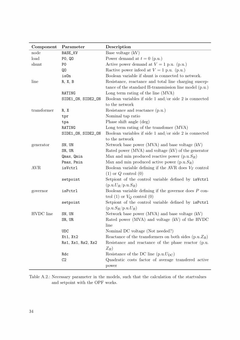
Component Parameter Descriptionnode BASE_KV Base voltage (kV)load P0, QO Power demand at t = 0 (p.u.)shunt P0 Active power demand at V = 1 p.u. (p.u.)
QO Ractive power infeed at V = 1 p.u. (p.u.)isOn Boolean variable if shunt is connected to network.
line R, X, B Resistance, reactance and total line charging suscep-tance of the standard Π-transmission line model (p.u.)
RATING Long term rating of the line (MVA)SIDE1_ON, SIDE2_ON Boolean variables if side 1 and/or side 2 is connected
to the networktransformer R, X Resistance and reactance (p.u.)
tpr Nominal tap ratiotpa Phase shift angle (deg)RATING Long term rating of the transfomer (MVA)SIDE1_ON, SIDE2_ON Boolean variables if side 1 and/or side 2 is connected
to the networkgenerator SN, UN Network base power (MVA) and base voltage (kV)
SR, UR Rated power (MVA) and voltage (kV) of the generatorQmax, Qmin Max and min produced reactive power (p.u.SR)Pmax, Pmin Max and min produced active power (p.u.SR)
AVR isVctrl Boolean variable defining if the AVR does VT control(1) or Q control (0)
setpoint Setpiont of the control variable defined by isVctrl(p.u.UR/p.u.SR)
governor isPctrl Boolean variable defining if the governor does P con-trol (1) or VQ control (0)
setpoint Setpiont of the control variable defined by isPctrl(p.u.SR/p.u.UR)
HVDC line SN, UN Network base power (MVA) and base voltage (kV)SR, UR Rated power (MVA) and voltage (kV) of the HVDC
lineUDC Nominal DC voltage (Not needed?)Xt1, Xt2 Reactance of the transformers on both sides (p.u.ZR)Rs1, Xs1, Rs2, Xs2 Resistance and reactance of the phase reactor (p.u.
ZR)Rdc Resistance of the DC line (p.u.UDC)C2 Quadratic costs factor of average transfered active
power
Table A.2.: Necessary parameter in the models, such that the calculation of the startvaluesand setpoint with the OPF works.
34
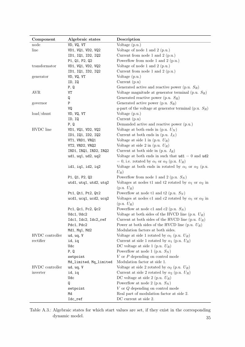
Component Algebraic states Descriptionnode VD, VQ, VT Voltage (p.u.)line VD1, VQ1, VD2, VQ2 Voltage of node 1 and 2 (p.u.)
ID1, IQ1, ID2, IQ2 Current from node 1 and 2 (p.u.)P1, Q1, P2, Q2 Powerflow from node 1 and 2 (p.u.)
transformator VD1, VQ1, VD2, VQ2 Voltage of node 1 and 2 (p.u.)ID1, IQ1, ID2, IQ2 Current from node 1 and 2 (p.u.)
generator VD, VQ, VT Voltage (p.u.)ID, IQ Current (p.u)P, Q Generated active and reactive power (p.u. SR)
AVR VT Voltage magnitude at generator terminal (p.u. SR)Q Generated reactive power (p.u. SR)
governor P Generated active power (p.u. SR)VQ q-part of the voltage at generator terminal (p.u. SR)
load/shunt VD, VQ, VT Voltage (p.u.)ID, IQ Current (p.u)P, Q Demanded active and reactive power (p.u.)
HVDC line VD1, VQ1, VD2, VQ2 Voltage at both ends in (p.u. UN )ID1, IQ1, ID2, IQ2 Current at both ends in (p.u. IN )VT1, VRD1, VRQ1 Voltage at side 1 in (p.u. UR)VT2, VRD2, VRQ2 Voltage at side 2 in (p.u. UR)IRD1, IRQ1, IRD2, IRQ2 Current at both side in (p.u. IR)ud1, uq1, ud2, uq2 Voltage at both ends in such that ud1 = 0 and ud2
= 0, i.e. rotated by α1 or α2 (p.u. UR)id1, iq1, id2, iq2 Voltage at both ends in rotated by α1 or α2 (p.u.
UR)P1, Q1, P2, Q2 Powerflow from node 1 and 2 (p.u. SN )utd1, utq1, utd2, utq2 Voltages at nodes t1 and t2 rotated by α1 or α2 in
(p.u. UR)Pt1, Qt1, Pt2, Qt2 Powerflow at node t1 and t2 (p.u. SN )ucd1, ucq1, ucd2, ucq2 Voltages at nodes c1 and c2 rotated by α1 or α2 in
(p.u. UR)Pc1, Qc1, Pc2, Qc2 Powerflow at node c1 and c2 (p.u. SN )Udc1, Udc2 Voltage at both sides of the HVCD line (p.u. UR)Idc1, Idc2, Idc2_ref Current at both sides of the HVCD line (p.u. UR)Pdc1, Pdc2 Power at both sides of the HVCD line (p.u. UR)Md1, Mq1, Md2 Modulation factors at both sides.
HVDC controller ud, uq, V Voltage at side 1 rotated by α1 (p.u. UR)rectifier id, iq Current at side 1 rotated by α1 (p.u. UR)
Udc DC voltage at side 1 (p.u. UR)P, Q Powerflow at node 1 (p.u. SN )setpoint V or P depending on control modeMd_limited, Mq_limited Modulation factor at side 1.
HVDC controller ud, uq, V Voltage at side 2 rotated by α2 (p.u. UR)inverter id, iq Current at side 2 rotated by α2 (p.u. UR)
Udc DC voltage at side 2 (p.u. UR)Q Powerflow at node 2 (p.u. SN )setpoint V or Q depending on control modeMd Real part of modulation factor at side 2.Idc_ref DC current at side 2.
Table A.3.: Algebraic states for which start values are set, if they exist in the correspondingdynamic model. 35
Component Setpoints Type DescriptionHVDC controllerrectifier
dPset dynstate Active power flow at node 1 (p.u.SR)
dsetpiont dynstate Reactove power flow at node 1 (p.u.SR) if PQcontrol, voltage magnitude at node 1 (p.uUR)if PV control.
HVDC controllerinverter
dsetpiont dynstate Reactive power flow at node 2 (p.u.SR) ifUDCQ control, voltage magnitude at node 2(p.uUR) if UDCV control.
UDC_set param Set point of the DC voltage (p.u.UR)AVR setpoint param Voltage magnitude at generator bus (p.u.UN )
if V control, reactive power (p.u.SN ) ifQ con-trol.
governor setpiont param Active power (p.u.SN ) if P control, Vq at gen-erator bus (p.u.UN ) if V control
Table A.4.: Set points of controllers modified by setpoints_and_start_values. Type isspecifying if a set point is implemented as dynamic state or parameter. The setpoints of the AVRs and governors are only modified if the production of generatorswas optimized in the OPF calculation as well, i.e. isPF = 0.
CTRLTYPE ctrl vars0 P, Q1 P, V
Table A.5.: Rectifier controller types (controller at side 1).
CTRLTYPE ctrl vars0 Q, UDC1 V, UDC
Table A.6.: Inverter controller types (controller at side 2).
isVctrl ctrl vars0 Q1 VT
Table A.7.: AVR controller types.
isPctrl ctrl vars0 VQ1 P
Table A.8.: Governor controller types.
36
B. Simulation Parameters
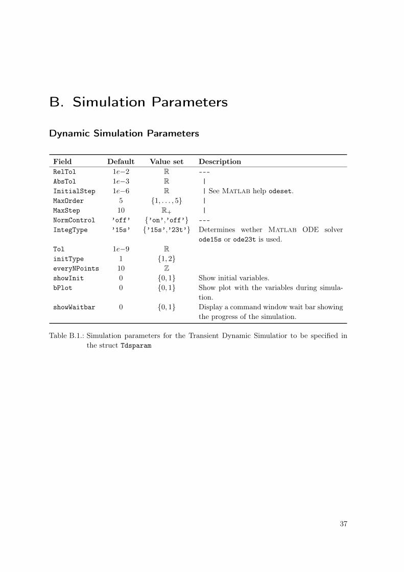
Dynamic Simulation Parameters
Field Default Value set DescriptionRelTol 1e−2 R –––AbsTol 1e−3 R |InitialStep 1e−6 R | See Matlab help odeset.MaxOrder 5 1, . . . , 5 |MaxStep 10 R+ |NormControl ’off’ ’on’,’off’ –––IntegType ’15s’ ’15s’,’23t’ Determines wether Matlab ODE solver
ode15s or ode23t is used.Tol 1e−9 RinitType 1 1, 2everyNPoints 10 ZshowInit 0 0, 1 Show initial variables.bPlot 0 0, 1 Show plot with the variables during simula-
tion.showWaitbar 0 0, 1 Display a command window wait bar showing
the progress of the simulation.
Table B.1.: Simulation parameters for the Transient Dynamic Simulatior to be specified inthe struct Tdsparam
37
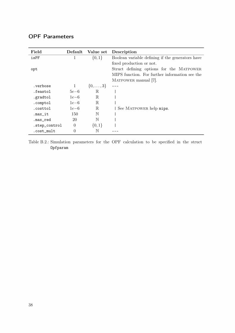
OPF Parameters
Field Default Value set DescriptionisPF 1 0, 1 Boolean variable defining if the generators have
fixed production or not.opt Struct defining options for the Matpower
MIPS function. For further information see theMatpower manual [7].
.verbose 1 0, . . . , 3 –––
.feastol 5e−6 R |
.gradtol 1e−6 R |
.comptol 1e−6 R |
.costtol 1e−6 R | See Matpower help mips.
.max_it 150 N |
.max_red 20 N |
.step_control 0 0, 1 |
.cost_mult 0 N –––
Table B.2.: Simulation parameters for the OPF calculation to be specified in the structOpfparam
38
C. Test System
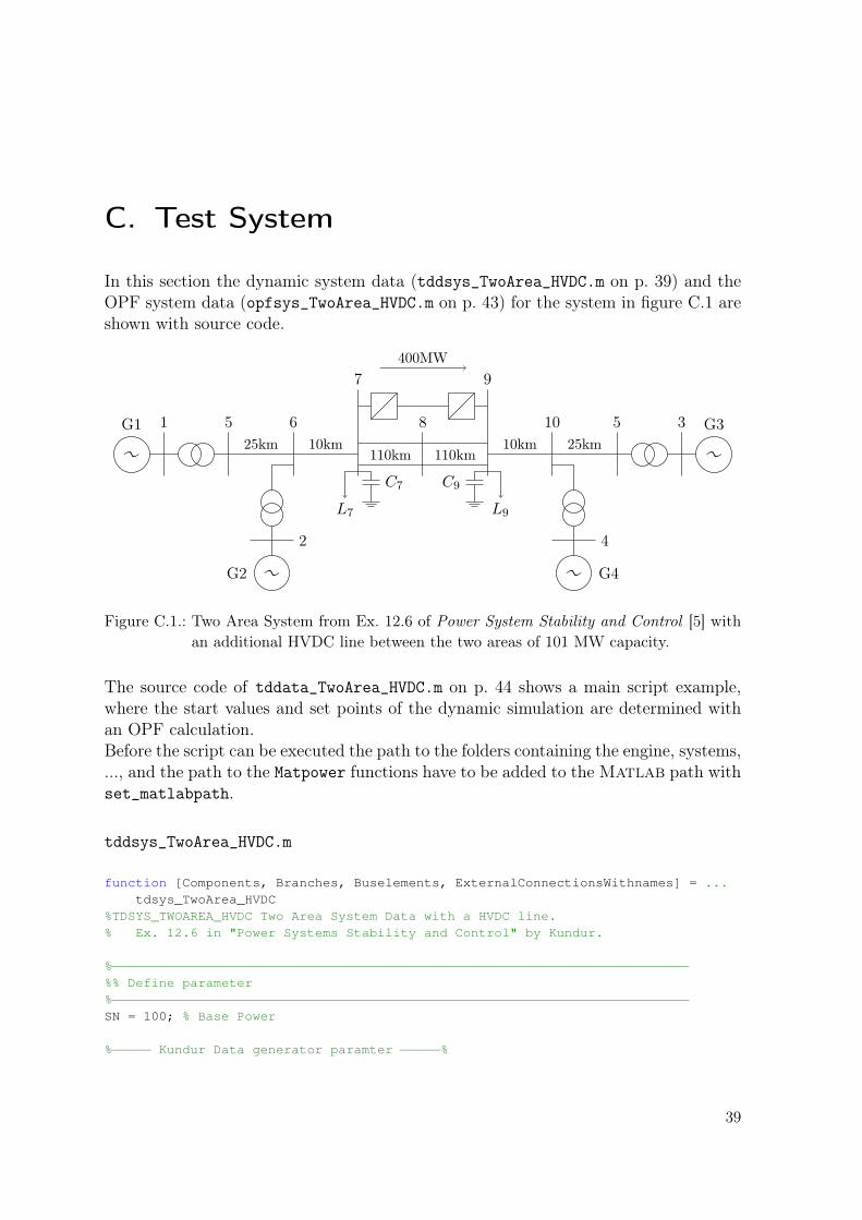
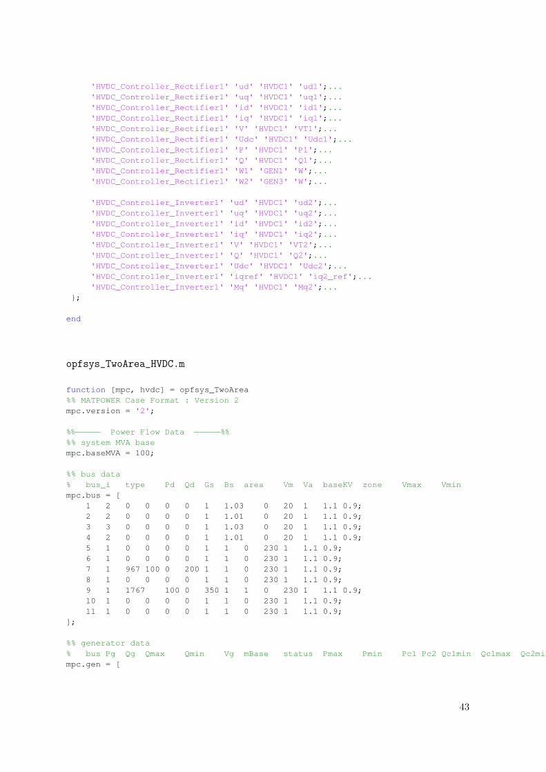
In this section the dynamic system data (tddsys_TwoArea_HVDC.m on p. 39) and theOPF system data (opfsys_TwoArea_HVDC.m on p. 43) for the system in figure C.1 areshown with source code.
1 5 6
7
8
9
10 5 3
2 4
400MW
110km 110km10km25km 10km 25km
L7 L9
C7 C9
~G1
~G3
~ G4~G2
Figure C.1.: Two Area System from Ex. 12.6 of Power System Stability and Control [5] withan additional HVDC line between the two areas of 101 MW capacity.
The source code of tddata_TwoArea_HVDC.m on p. 44 shows a main script example,where the start values and set points of the dynamic simulation are determined withan OPF calculation.Before the script can be executed the path to the folders containing the engine, systems,..., and the path to the Matpower functions have to be added to the Matlab path withset_matlabpath.
tddsys_TwoArea_HVDC.m
function [Components, Branches, Buselements, ExternalConnectionsWithnames] = ...tdsys_TwoArea_HVDC
%TDSYS_TWOAREA_HVDC Two Area System Data with a HVDC line.% Ex. 12.6 in "Power Systems Stability and Control" by Kundur.
%−−−−−−−−−−−−−−−−−−−−−−−−−−−−−−−−−−−−−−−−−−−−−−−−−−−−−−−−−−−−−−−−−−−−−−−−−−%% Define parameter%−−−−−−−−−−−−−−−−−−−−−−−−−−−−−−−−−−−−−−−−−−−−−−−−−−−−−−−−−−−−−−−−−−−−−−−−−−SN = 100; % Base Power
%−−−−− Kundur Data generator paramter −−−−−%
39
Ra = 0.0025;Ll = 0.2;Xd = 1.8;Xq = 1.7;Xd1 = 0.3;Xq1 = 0.55;Xd2 = 0.25;Xq2 = 0.25;Td1 = 8.0;Tq1 = 0.4;Td2 = 0.03;Tq2 = 0.05;H(1:2) = 6.5;H(3:4) = 6.175;ws = 2*pi*60;KD = 0;
%−−−−− HVDC parameters −−−−−%SR = 101;UR = 230;UN = 230;UDC = 80;X_trafo = 0.113;X_reactor = 0.1656;R = 0.001;Rdc = 1.1568E−03;Cdc_conv = 3.9731E−03;Cdc = 9.7584E−06;Ldc = 2.2094E−06;l=220;f=2000;w1 = 2*pi*60;w2 = 2*pi*60;K0 = sqrt(2)*sqrt(3)/pi;C2 = 0; % Quadratic cost of HVDC line f = C2*(PN1+PN2)^2
%−−−−− HVDC controller −−−−−%CTRLTYPE = [1 1]; % 0: PQ−ctrl 1: PV−ctrl / 0: QUdc−ctrl 1: VUdc−ctrlUdc2_set = 1;idref_MIN = −0.5;idref_MAX = 0.5;T_P = 0.1;T_Q = 0.1;Kp_Udc = 100;Ki_Udc = 10000;Kp_i = 0.01 ;Ki_i = 0.02;Kp_P = 0.5;Ki_P = 50;Kp_Q1 = 10;Ki_Q1 = 1e3;Kp_Q2 = Kp_Q1;Ki_Q2 = Kp_Q2;
%−−−−−−−−−−−−−−−−−−−−−−−−−−−−−−−−−−−−−−−−−−−−−−−−−−−−−−−−−−−−−−−−−−−−−−−−−−
40
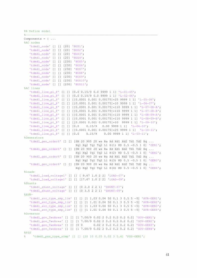
%% Define model%−−−−−−−−−−−−−−−−−−−−−−−−−−−−−−−−−−−−−−−−−−−−−−−−−−−−−−−−−−−−−−−−−−−−−−−−−−Components = ...%AC nodes
'tdmdl_node' [] [] [20] 'BUS1';'tdmdl_node' [] [] [20] 'BUS2';'tdmdl_node' [] [] [20] 'BUS3';'tdmdl_node' [] [] [20] 'BUS4';'tdmdl_node' [] [] [230] 'BUS5';'tdmdl_node' [] [] [230] 'BUS6';'tdmdl_node' [] [] [230] 'BUS7';'tdmdl_node' [] [] [230] 'BUS8';'tdmdl_node' [] [] [230] 'BUS9';'tdmdl_node' [] [] [230] 'BUS10';'tdmdl_node' [] [] [230] 'BUS11';
%AC lines'tdmdl_line_pi_P' [] [] [0.0 0.15/9 0.0 9999 1 1] 'L−01−05';'tdmdl_line_pi_P' [] [] [0.0 0.15/9 0.0 9999 1 1] 'L−02−06';'tdmdl_line_pi_P' [] [] [[0.0001 0.001 0.00175]*25 9999 1 1] 'L−05−06';'tdmdl_line_pi_P' [] [] [[0.0001 0.001 0.00175]*10 9999 1 1] 'L−06−07';'tdmdl_line_pi_P' [] [] [[0.0001 0.001 0.00175]*110 9999 1 1] 'L−07−08−A';'tdmdl_line_pi_P' [] [] [[0.0001 0.001 0.00175]*110 9999 1 1] 'L−07−08−B';'tdmdl_line_pi_P' [] [] [[0.0001 0.001 0.00175]*110 9999 1 1] 'L−08−09−A';'tdmdl_line_pi_P' [] [] [[0.0001 0.001 0.00175]*110 9999 1 1] 'L−08−09−B';'tdmdl_line_pi_P' [] [] [[0.0001 0.001 0.00175]*10 9999 1 1] 'L−09−10';'tdmdl_line_pi_P' [] [] [0.0 0.15/9 0.00 9999 1 1] 'L−04−10';'tdmdl_line_pi_P' [] [] [[0.0001 0.001 0.00175]*25 9999 1 1] 'L−10−11';'tdmdl_line_pi_P' [] [] [0.0 0.15/9 0.00 9999 1 1] 'L−03−11';
%Generators'tdmdl_gen_order6' [] [] [SN 20 900 20 ws Ra Xd Xd1 Xd2 Td1 Td2 Xq ...
Xq1 Xq2 Tq1 Tq2 Ll H(1) KD 0.5 −0.5 1 0] 'GEN1';'tdmdl_gen_order6' [] [] [SN 20 900 20 ws Ra Xd Xd1 Xd2 Td1 Td2 Xq ...
Xq1 Xq2 Tq1 Tq2 Ll H(2) KD 0.5 −0.5 1 0] 'GEN2';'tdmdl_gen_order6' [] [] [SN 20 900 20 ws Ra Xd Xd1 Xd2 Td1 Td2 Xq ...
Xq1 Xq2 Tq1 Tq2 Ll H(3) KD 0.5 −0.5 1 0] 'GEN3';'tdmdl_gen_order6' [] [] [SN 20 900 20 ws Ra Xd Xd1 Xd2 Td1 Td2 Xq ...
Xq1 Xq2 Tq1 Tq2 Ll H(4) KD 0.5 −0.5 1 0] 'GEN4';%Loads
'tdmdl_load_voltage1' [] [] [ 9.67 1.0 2 2] 'LOAD−07';'tdmdl_load_voltage1' [] [] [17.67 1.0 2 2] 'LOAD−09';
%Shunts'tdmdl_shunt_voltage' [] [] [0 2.0 2 2 1] 'SHUNT−07';'tdmdl_shunt_voltage' [] [] [0 3.5 2 2 1] 'SHUNT−09';
%AVR−'tdmdl_avr_type_smp_lim' [] [] [1 1.03 0.04 50 0.1 3 0.5 5 −5] 'AVR−GEN1';'tdmdl_avr_type_smp_lim' [] [] [1 1.01 0.04 50 0.1 3 0.5 5 −5] 'AVR−GEN2';'tdmdl_avr_type_smp_lim' [] [] [1 1.03 0.04 50 0.1 3 0.5 5 −5] 'AVR−GEN3';'tdmdl_avr_type_smp_lim' [] [] [1 1.01 0.04 50 0.1 3 0.5 5 −5] 'AVR−GEN4';
%Governor'tdmdl_gov_TwoArea' [] [] [1 7.00/9 0.02 2 0.2 0.2 0.2 0.2] 'GOV−GEN1';'tdmdl_gov_TwoArea' [] [] [1 7.00/9 0.02 2 0.2 0.2 0.2 0.2] 'GOV−GEN2';'tdmdl_gov_TwoArea' [] [] [0 0 0.02 2 0.2 0.2 0.2 0.2] 'GOV−GEN3';'tdmdl_gov_TwoArea' [] [] [1 7.00/9 0.02 2 0.2 0.2 0.2 0.2] 'GOV−GEN4';
%PSS% 'tdmdl_pss_type_simp' [] [] [20 10 0.05 0.02 3 5.4] 'PSS−GEN1';
41
% 'tdmdl_pss_type_simp' [] [] [20 10 0.05 0.02 3 5.4] 'PSS−GEN2';% 'tdmdl_pss_type_simp' [] [] [20 10 0.05 0.02 3 5.4] 'PSS−GEN3';% 'tdmdl_pss_type_simp' [] [] [20 10 0.05 0.02 3 5.4] 'PSS−GEN4';%HVDC1
'tdmdl_hvdc_physical_ModulationIndex3' [] [] [SN UN SR UR UDC ...X_trafo X_reactor R X_trafo X_reactor R l*Rdc (l*Cdc+Cdc_conv) ...l*Ldc f w1 w2 K0 C2] 'HVDC1';
'tdmdl_hvdc_controller_rectifier_ModulationIndex5' [] [] [X_trafo ...X_reactor K0 Kp_i Ki_i Kp_P Ki_P CTRLTYPE(1) Kp_Q1 Ki_Q1 T_P ...T_Q idref_MIN idref_MAX 150 20 0.05] 'HVDC_Controller_Rectifier1';
'tdmdl_hvdc_controller_inverter_ModulationIndex5' [] [] [X_trafo ...X_reactor K0 Kp_i Ki_i CTRLTYPE(2) Kp_Q2 Ki_Q2 Udc2_set Kp_Udc ...Ki_Udc T_Q idref_MIN idref_MAX] 'HVDC_Controller_Inverter1';
;
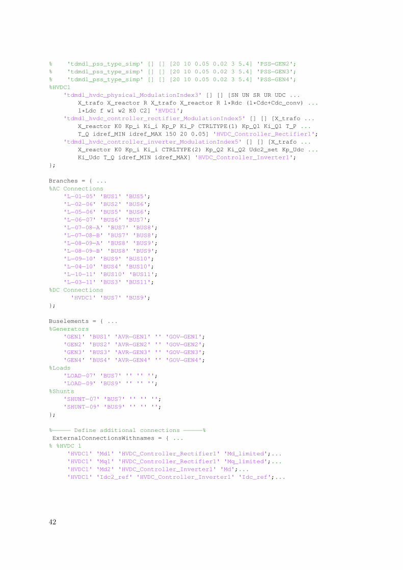
Branches = ...%AC Connections
'L−01−05' 'BUS1' 'BUS5';'L−02−06' 'BUS2' 'BUS6';'L−05−06' 'BUS5' 'BUS6';'L−06−07' 'BUS6' 'BUS7';'L−07−08−A' 'BUS7' 'BUS8';'L−07−08−B' 'BUS7' 'BUS8';'L−08−09−A' 'BUS8' 'BUS9';'L−08−09−B' 'BUS8' 'BUS9';'L−09−10' 'BUS9' 'BUS10';'L−04−10' 'BUS4' 'BUS10';'L−10−11' 'BUS10' 'BUS11';'L−03−11' 'BUS3' 'BUS11';
%DC Connections'HVDC1' 'BUS7' 'BUS9';
;
Buselements = ...%Generators
'GEN1' 'BUS1' 'AVR−GEN1' '' 'GOV−GEN1';'GEN2' 'BUS2' 'AVR−GEN2' '' 'GOV−GEN2';'GEN3' 'BUS3' 'AVR−GEN3' '' 'GOV−GEN3';'GEN4' 'BUS4' 'AVR−GEN4' '' 'GOV−GEN4';
%Loads'LOAD−07' 'BUS7' '' '' '';'LOAD−09' 'BUS9' '' '' '';
%Shunts'SHUNT−07' 'BUS7' '' '' '';'SHUNT−09' 'BUS9' '' '' '';
;
%−−−−− Define additional connections −−−−−%ExternalConnectionsWithnames = ...
% %HVDC 1'HVDC1' 'Md1' 'HVDC_Controller_Rectifier1' 'Md_limited';...'HVDC1' 'Mq1' 'HVDC_Controller_Rectifier1' 'Mq_limited';...'HVDC1' 'Md2' 'HVDC_Controller_Inverter1' 'Md';...'HVDC1' 'Idc2_ref' 'HVDC_Controller_Inverter1' 'Idc_ref';...
42
'HVDC_Controller_Rectifier1' 'ud' 'HVDC1' 'ud1';...'HVDC_Controller_Rectifier1' 'uq' 'HVDC1' 'uq1';...'HVDC_Controller_Rectifier1' 'id' 'HVDC1' 'id1';...'HVDC_Controller_Rectifier1' 'iq' 'HVDC1' 'iq1';...'HVDC_Controller_Rectifier1' 'V' 'HVDC1' 'VT1';...'HVDC_Controller_Rectifier1' 'Udc' 'HVDC1' 'Udc1';...'HVDC_Controller_Rectifier1' 'P' 'HVDC1' 'P1';...'HVDC_Controller_Rectifier1' 'Q' 'HVDC1' 'Q1';...'HVDC_Controller_Rectifier1' 'W1' 'GEN1' 'W';...'HVDC_Controller_Rectifier1' 'W2' 'GEN3' 'W';...
'HVDC_Controller_Inverter1' 'ud' 'HVDC1' 'ud2';...'HVDC_Controller_Inverter1' 'uq' 'HVDC1' 'uq2';...'HVDC_Controller_Inverter1' 'id' 'HVDC1' 'id2';...'HVDC_Controller_Inverter1' 'iq' 'HVDC1' 'iq2';...'HVDC_Controller_Inverter1' 'V' 'HVDC1' 'VT2';...'HVDC_Controller_Inverter1' 'Q' 'HVDC1' 'Q2';...'HVDC_Controller_Inverter1' 'Udc' 'HVDC1' 'Udc2';...'HVDC_Controller_Inverter1' 'iqref' 'HVDC1' 'iq2_ref';...'HVDC_Controller_Inverter1' 'Mq' 'HVDC1' 'Mq2';...
;
end
opfsys_TwoArea_HVDC.m
function [mpc, hvdc] = opfsys_TwoArea%% MATPOWER Case Format : Version 2mpc.version = '2';
%%−−−−− Power Flow Data −−−−−%%%% system MVA basempc.baseMVA = 100;
%% bus data% bus_i type Pd Qd Gs Bs area Vm Va baseKV zone Vmax Vminmpc.bus = [
1 2 0 0 0 0 1 1.03 0 20 1 1.1 0.9;2 2 0 0 0 0 1 1.01 0 20 1 1.1 0.9;3 3 0 0 0 0 1 1.03 0 20 1 1.1 0.9;4 2 0 0 0 0 1 1.01 0 20 1 1.1 0.9;5 1 0 0 0 0 1 1 0 230 1 1.1 0.9;6 1 0 0 0 0 1 1 0 230 1 1.1 0.9;7 1 967 100 0 200 1 1 0 230 1 1.1 0.9;8 1 0 0 0 0 1 1 0 230 1 1.1 0.9;9 1 1767 100 0 350 1 1 0 230 1 1.1 0.9;10 1 0 0 0 0 1 1 0 230 1 1.1 0.9;11 1 0 0 0 0 1 1 0 230 1 1.1 0.9;
];
%% generator data% bus Pg Qg Qmax Qmin Vg mBase status Pmax Pmin Pc1 Pc2 Qc1min Qc1max Qc2min Qc2max ramp_agc ramp_10 ramp_30 ramp_q apfmpc.gen = [
43
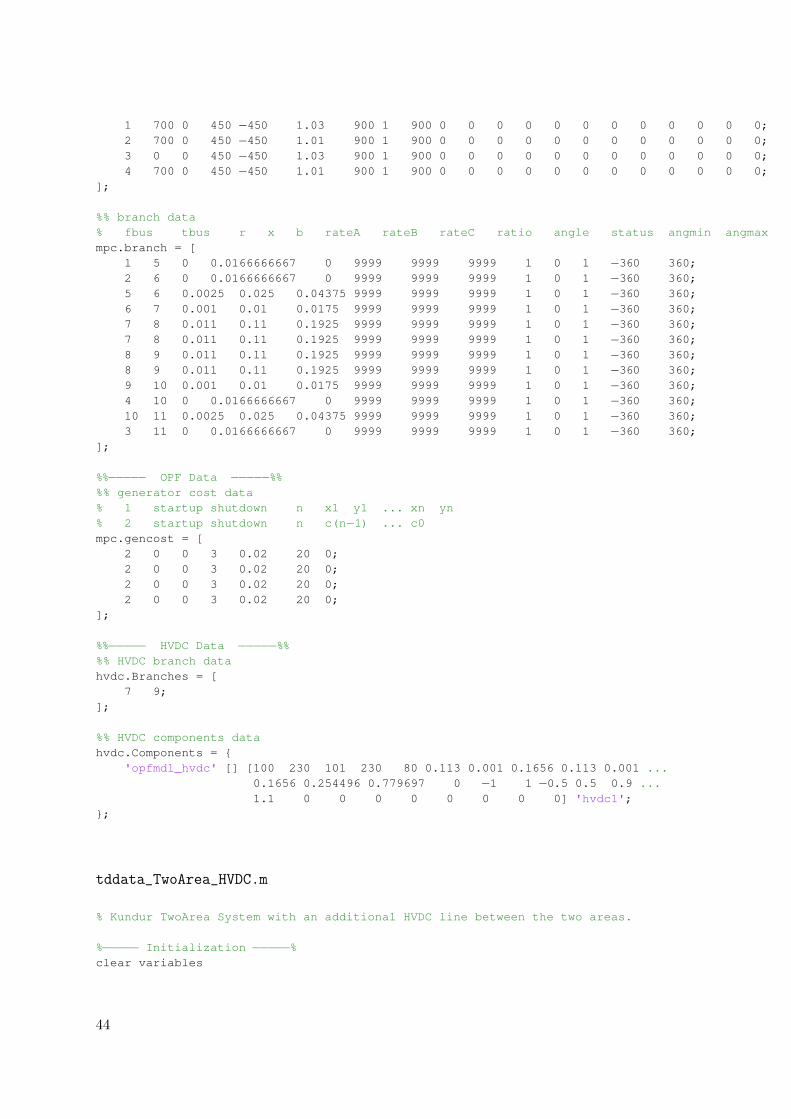
1 700 0 450 −450 1.03 900 1 900 0 0 0 0 0 0 0 0 0 0 0 0;2 700 0 450 −450 1.01 900 1 900 0 0 0 0 0 0 0 0 0 0 0 0;3 0 0 450 −450 1.03 900 1 900 0 0 0 0 0 0 0 0 0 0 0 0;4 700 0 450 −450 1.01 900 1 900 0 0 0 0 0 0 0 0 0 0 0 0;
];
%% branch data% fbus tbus r x b rateA rateB rateC ratio angle status angmin angmaxmpc.branch = [
1 5 0 0.0166666667 0 9999 9999 9999 1 0 1 −360 360;2 6 0 0.0166666667 0 9999 9999 9999 1 0 1 −360 360;5 6 0.0025 0.025 0.04375 9999 9999 9999 1 0 1 −360 360;6 7 0.001 0.01 0.0175 9999 9999 9999 1 0 1 −360 360;7 8 0.011 0.11 0.1925 9999 9999 9999 1 0 1 −360 360;7 8 0.011 0.11 0.1925 9999 9999 9999 1 0 1 −360 360;8 9 0.011 0.11 0.1925 9999 9999 9999 1 0 1 −360 360;8 9 0.011 0.11 0.1925 9999 9999 9999 1 0 1 −360 360;9 10 0.001 0.01 0.0175 9999 9999 9999 1 0 1 −360 360;4 10 0 0.0166666667 0 9999 9999 9999 1 0 1 −360 360;10 11 0.0025 0.025 0.04375 9999 9999 9999 1 0 1 −360 360;3 11 0 0.0166666667 0 9999 9999 9999 1 0 1 −360 360;
];
%%−−−−− OPF Data −−−−−%%%% generator cost data% 1 startup shutdown n x1 y1 ... xn yn% 2 startup shutdown n c(n−1) ... c0mpc.gencost = [
2 0 0 3 0.02 20 0;2 0 0 3 0.02 20 0;2 0 0 3 0.02 20 0;2 0 0 3 0.02 20 0;
];
%%−−−−− HVDC Data −−−−−%%%% HVDC branch datahvdc.Branches = [
7 9;];
%% HVDC components datahvdc.Components =
'opfmdl_hvdc' [] [100 230 101 230 80 0.113 0.001 0.1656 0.113 0.001 ...0.1656 0.254496 0.779697 0 −1 1 −0.5 0.5 0.9 ...1.1 0 0 0 0 0 0 0 0] 'hvdc1';
;
tddata_TwoArea_HVDC.m
% Kundur TwoArea System with an additional HVDC line between the two areas.
%−−−−− Initialization −−−−−%clear variables
44
close all
%−−−−−−−−−−−−−−−−−−−−−−−−−−−−−−−−−−−−−−−−−−−−−−−−−−−−−−−−−−−−−−−−−−−−−−−−−−%% Define case and settings%−−−−−−−−−−−−−−−−−−−−−−−−−−−−−−−−−−−−−−−−−−−−−−−−−−−−−−−−−−−−−−−−−−−−−−−−−−%−−−−− Simulation settings −−−−−%tfinal = 0; % Calculation time (in seconds)isPlotting = 0; % Make plotsuseMPC = 0; % Model predictive control for HVDC controllersisSaving = 1; % Save results
if isSavingsavepath = [get_main_folder_path, 'Saves/'];casename = ['TIME_',int2str(tfinal), '_TwoArea_HVDC']; % Name of simulationTdsparam.savepath = [savepath, casename];
end
%−−−−− Dynamic simulation parameters −−−−−%Tdsparam.showInit = 1; % Show initial conditions: 1 show; 0 don't showTdsparam.showWaitbar = 1; % Show waitbar: 1 show; 0 don't show
%−−−−− OPF simulation paramters −−−−−%Opfparam.isPF = 1; % 1: Fixed generators (default) / 0: Flexible generators
%−−−−− System −−−−−%[Components, Branches, Buselements, ExternalConnectionsWithnames, x, OpfModel] = ...
load_system_with_opf_startvalues('tdsys_TwoArea_HVDC', Opfparam);
%−−−−− Disturbances −−−−−%Disturbances = ...
.49,'L−07−08−A','SIDE1_ON',0; ...
.55,'L−07−08−A','SIDE2_ON',0; ...;
%−−−−− MPC −−−−−%if useMPC
sampleTime = .1; % mpc sample time (in seconds)Mpcparam.sampleTime = sampleTime;Mpcparam.predictionTime = sampleTime; % mpc prediction time sample (seconds)Mpcparam.N = 10; % mpc horizonMpcparam.Tlin = 2;Mpcparam.Pmax_pu= .9;Mpcparam.Qmax_pu= .5;Mpcparam.dmaxP = .1;Mpcparam.dmaxQ = .1;
%−−−−− Add MPC block to Components −−−−−%modelmpc.sampletime = sampleTime;modelmpc.funcname = 'my_empty_mpc_function';Components(size(Components,1)+1,1:5) = ...
'tdm_block_sample_system' [] [] [modelmpc] 'SAMPLE';
%−−−−− Controller States/Output −−−−−%Mpcparam.ControllerStates = controller_states(Components);
45
Mpcparam.ControllerOutput = controller_output(Components);
else
Mpcparam = struct([]);
end
%−−−−− Define variables to record and to plot −−−−−%Records = [ ...
default_var_lines(Components);default_var_nodes(Components);default_var_gens(Components);default_var_loads(Components);default_var_hvdc(Components);records_for_compare_start_values(Components);];
Plots = [ ...plot_line('L−07−08−A');plot_line('L−07−08−B');];
RecordVars = merge_records_with_plots(Records, Plots, Components);
%−−−−−−−−−−−−−−−−−−−−−−−−−−−−−−−−−−−−−−−−−−−−−−−−−−−−−−−−−−−−−−−−−−−−−−−−−−%% Run dynamic simulation%−−−−−−−−−−−−−−−−−−−−−−−−−−−−−−−−−−−−−−−−−−−−−−−−−−−−−−−−−−−−−−−−−−−−−−−−−−Model = run_dynamic_simulation(tfinal, Components, Branches, Buselements, ...
ExternalConnectionsWithnames, Disturbances, RecordVars, Tdsparam, ...Mpcparam);
%−−−−− Compare values before and after initialization run −−−−−%compare_start_values(x, OpfModel, Model, Components, Branches, ...
Buselements, ExternalConnectionsWithnames, 1e−6);
%−−−−−−−−−−−−−−−−−−−−−−−−−−−−−−−−−−−−−−−−−−−−−−−−−−−−−−−−−−−−−−−−−−−−−−−−−−%% Plot/save results%−−−−−−−−−−−−−−−−−−−−−−−−−−−−−−−−−−−−−−−−−−−−−−−−−−−−−−−−−−−−−−−−−−−−−−−−−−Model.results.map = make_resultsmap(Model);
%−−−−− Plot results −−−−−%if isPlotting
draw_plots(Model, Plots);end
%−−−−− Save results −−−−−%Model.disturbances = Disturbances;Model.results.plotfnc = Plots;if isSaving
save([savepath, casename],'Model')end
%−−−−− Clear variables −−−−−%clearvars −except Model
46
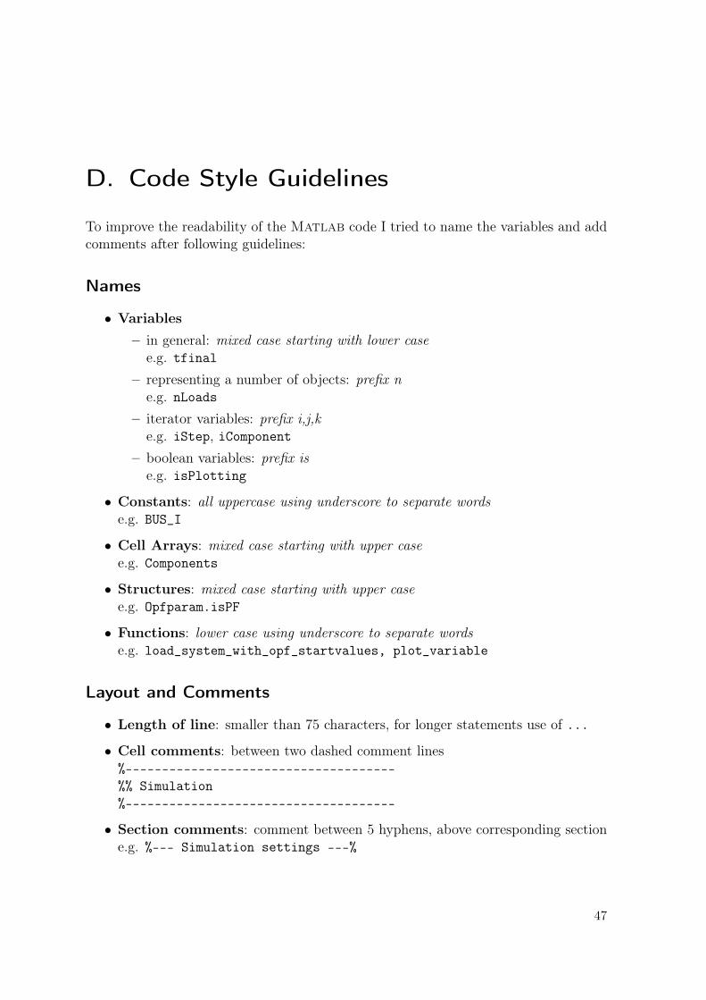
D. Code Style Guidelines
To improve the readability of the Matlab code I tried to name the variables and addcomments after following guidelines:
Names
• Variables– in general: mixed case starting with lower case
e.g. tfinal– representing a number of objects: prefix n
e.g. nLoads– iterator variables: prefix i,j,k
e.g. iStep, iComponent– boolean variables: prefix is
e.g. isPlotting
• Constants: all uppercase using underscore to separate wordse.g. BUS_I
• Cell Arrays: mixed case starting with upper casee.g. Components
• Structures: mixed case starting with upper casee.g. Opfparam.isPF
• Functions: lower case using underscore to separate wordse.g. load_system_with_opf_startvalues, plot_variable
Layout and Comments
• Length of line: smaller than 75 characters, for longer statements use of ...
• Cell comments: between two dashed comment lines%–––––––––––––––––––––––––––––––––––––%% Simulation%–––––––––––––––––––––––––––––––––––––
• Section comments: comment between 5 hyphens, above corresponding sectione.g. %––- Simulation settings ––-%
47

List of Figures
2.1. HVDC model for optimal power flow calculations. . . . . . . . . . . . . 102.2. Description of dynamic behavior with a set of differential- and algebraic
equations and discrete events. . . . . . . . . . . . . . . . . . . . . . . . 122.3. Description of dynamic behavior with a set of differential- and algebraic
equations and discrete events modeled with a change in the parameter λ. 12
3.1. Flow diagram of the combined simulator. The grey shaded boxes arethe before existing simulators, while the white boxes are implementedin the context of this thesis. tdsys is the system data for the dynamicsimulation and opfsys is the system data for the OPF. Furthermore, xis the resulting system state of the OPF calculation and Model containsinformation about the dynamic simulation, in particular the recordedvalues. . . . . . . . . . . . . . . . . . . . . . . . . . . . . . . . . . . . . 13
3.2. Flow diagram with the functions concerning record and plot manage-ment. The asterisks are placeholders for one of gens, hvdc, lines,loads, nodes. . . . . . . . . . . . . . . . . . . . . . . . . . . . . . . . . 23
4.1. Optimal set points of the HVDC line in the Two Area System whengenerators have fixed production profile. . . . . . . . . . . . . . . . . . 28
C.1. Two Area System from Ex. 12.6 of Power System Stability and Control[5] with an additional HVDC line between the two areas of 101 MWcapacity. . . . . . . . . . . . . . . . . . . . . . . . . . . . . . . . . . . . 39
49


List of Tables
4.1. Initialization with start values compared to initialization with flat start.Required time (arithmetic mean of 100 initialization runs) and requirednumber of iterations. . . . . . . . . . . . . . . . . . . . . . . . . . . . . 28
A.1. Model naming convention for the dynamic models. * indicates that onlythe prefix has to match. . . . . . . . . . . . . . . . . . . . . . . . . . . 33
A.2. Necessary parameter in the models, such that the calculation of thestartvalues and setpoint with the OPF works. . . . . . . . . . . . . . . 34
A.3. Algebraic states for which start values are set, if they exist in the corre-sponding dynamic model. . . . . . . . . . . . . . . . . . . . . . . . . . 35
A.4. Set points of controllers modified by setpoints_and_start_values.Type is specifying if a set point is implemented as dynamic state orparameter. The set points of the AVRs and governors are only modifiedif the production of generators was optimized in the OPF calculation aswell, i.e. isPF = 0. . . . . . . . . . . . . . . . . . . . . . . . . . . . . . 36
A.5. Rectifier controller types (controller at side 1). . . . . . . . . . . . . . . 36A.6. Inverter controller types (controller at side 2). . . . . . . . . . . . . . . 36A.7. AVR controller types. . . . . . . . . . . . . . . . . . . . . . . . . . . . . 36A.8. Governor controller types. . . . . . . . . . . . . . . . . . . . . . . . . . 36
B.1. Simulation parameters for the Transient Dynamic Simulatior to be spec-ified in the struct Tdsparam . . . . . . . . . . . . . . . . . . . . . . . . 37
B.2. Simulation parameters for the OPF calculation to be specified in thestruct Opfparam . . . . . . . . . . . . . . . . . . . . . . . . . . . . . . . 38
51


![Overview of the Configuration and Power Converters in High ... · Fig. 8. Basic scheme of the LCC-HVDC and VSC-HVDC transmission system [6]. Comparison of the CSC-HVDC and VSC-HVDC](https://img.pdfslide.us/doc/110x75/5ebc0e8dd027f5592e56ad65/overview-of-the-configuration-and-power-converters-in-high-fig-8-basic-scheme.jpg)