Vorticity Equation, Current Conservation and the Solutions

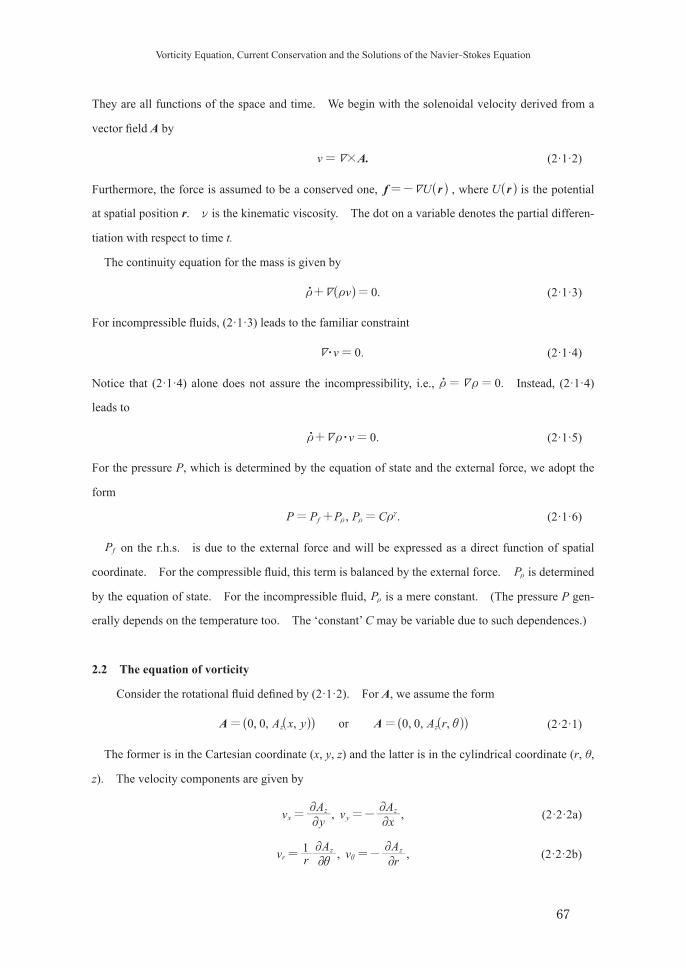
Vorticity Equation, Current Conservation and the Solutions of the Navier-Stokes Equation

65

【Article】


TAKAHASHI Koichi

Abstract　The motion of a Newtonian fluid is described by the Navier-Stokes equation, which is a partial differential equation for the velocity field with respect to space and time variables.　Its nonlinearity is the source of difficulty in finding general solutions.　In this paper, a method of determining the velocity fields in the Navier-Stokes equation is proposed by noting a similarity of the vorticity equation in two dimensions to the current conservation equation.　By noting this correspondence, the original Navier-Stokes equation for flows of one degree of freedom is trans-formed to a linear partial differential equation with respect to space variables only.　Some exact two-dimensional solutions including well-known ones are derived by this method.　The solu-tions for swirling flows together with its perturbation can be a model of typhoon.Key words : Navier-Stokes equation, continuity equation, exact solutions, typhoon

1.　Introduction

The dynamics of the Newtonian fluid is governed by the Navier-Stokes equation, the continuity

equation and the equation of state.　The first two are the non-linear partial differential equations with

respect to space and time.　Together with the absence of any internal symmetry, finding ‘exact’ solu-

tions in a general way is very difficult.　Many exact solutions have been found so far by imposing

various physical requirements on the boundary conditions, the degrees of freedom and the global

properties of the fluid and its motions.　Incompressibility is one of the conditions customarily

adopted in literatures.　For a review, see Wang (1991) and Drazin and Riley (2006).

On the other hand, owing to the development of the technique of numerical analyses, numerical

solutions of ordinary differential equation are now easily obtained with grate accuracies.　Therefore,

from a practical point of view, we may also regard transforming the Navier-Stokes equation to the

ordinary differential equations as equivalent to obtaining exact solutions.

Ever since the Navier-Stokes equation was discovered and studied by Navier (1827), Poisson

(1831), Saint-Venant (1843) and Stokes (1845), many efforts have been devoted to find exact solu-

東北学院大学教養学部論集　第 164号

66

tions or the ordinary differential equations under peculiar boundary conditions.　For rotational stream

in two-dimension that we are interested in this paper, Kampe de Feriet (1930, 1932) and Tsien (1943)

have found various exact solutions.　For a review, see Wang (1991).

One of the origins of difficulty of solving the Navier-Stokes equation lies in that one has to take

account of the continuity equation separately.　This situation is in contrast with the case of U(1) sym-

metric quantum mechanics or field theories, where the continuity of conserved quantity is automati-

cally fulfilled by the solution of the Schrödinger equation or field equations.　If one can take advan-

tage of such a property of the U(1) symmetric theories in solving the Navier-Stokes equation, finding

its solutions may be greatly helped.　

In this paper, we focus our attention to the exact solutions of the Navier-Stokes equation.　By the

‘exact’ solution, we here mean those that are expressed in terms of the well-known analytic functions,

ordinary differential equations or integrations to be easily performed by the numerical techniques.　

We shall present a method of finding exact two-dimensional solutions of the Navier-Stokes equation

by utilizing the property of the conserved current.　Such currents may be explicitly constructed, e.g.,

in the framework of any U(1) symmetric theories.　The point we are going to notice is a mathemati-

cal parallelism between the vorticity equation and the current conservation equation.　This parallel-

ism enables us to transmute a conserved current to the vorticity via an ordinary differential equation.　

The method will be shown to be entirely consistent with directly solving the Navier-Stokes equation.　

The customary constraint of incompressibility will generally be removed throughout our discussions.

In the next section, we elaborate the idea that leads to the transmutation equation.　In sec.3, some

applications of the transmutation equation are presented.　In sec.4, a way of extension of the method

to higher degrees of freedom is discussed.　Sec.5 is devoted to a summary.

2.　 Correspondence of the vorticity equation and the current conservation equation for the solenoidal fluid

2.1　The Navier-Stokes equation

The Navier-Stokes equation is the partial differential equation for the velocity field and is written as

follows :

(2·1·1)

v, t , P and f are the velocity field, mass density, pressure and external volume force, respectively.　

v v v v .P f31v v 2$ $+ = + +U UU U Uot

-o ^ ^h h


67

They are all functions of the space and time.　We begin with the solenoidal velocity derived from a

vector field A by

(2·1·2)

Furthermore, the force is assumed to be a conserved one, Uf r= U- ^ h , where U r^ h is the potential

at spatial position r.　o is the kinematic viscosity.　The dot on a variable denotes the partial differen-

tiation with respect to time t.　

The continuity equation for the mass is given by

(2·1·3)

For incompressible fluids, (2·1·3) leads to the familiar constraint

(2·1·4)

Notice that (2·1·4) alone does not assure the incompressibility, i.e., .0Ut t= =o 　Instead, (2·1·4)

leads to

(2·1·5)

For the pressure P, which is determined by the equation of state and the external force, we adopt the

form

(2·1·6)

Pf on the r.h.s.　is due to the external force and will be expressed as a direct function of spatial

coordinate.　For the compressible fluid, this term is balanced by the external force.　Pt is determined

by the equation of state.　For the incompressible fluid, Pt is a mere constant.　(The pressure P gen-

erally depends on the temperature too.　The ‘constant’ C may be variable due to such dependences.)

2.2　The equation of vorticity

　Consider the rotational fluid defined by (2·1·2).　For A, we assume the form

(2·2·1)

The former is in the Cartesian coordinate (x, y, z) and the latter is in the cylindrical coordinate (r, θ,

z).　The velocity components are given by

(2·2·2a)

(2·2·2b)

v A.#=U

v 0.+ =Ut to ^ h

.v 0$U =

.v 0$Ut t+ =o

, .P P P P Cf t= + =t tc

, , , , , ,A x y A r0 0 0 0orA Az z= = i^^ ^^hh hh

, ,v yA v x

Ax

zy

z

22

22

= =-

, ,v rA v r

A1r

z z

22

22

i= =-i


68

and vz=0.　Note that 0A$ =U and .v 0$U = 　Such an Az is called the stream function.　

The Navier-Stokes equation (2·1·1), when operated by #U on the both sides, yields for conserva-

tive force

(2·2·3a)

(2·2·3b)

Here, ζ is the z component of the vorticity, i.e., , ,v 0 0#U/~ g=^ h defined by

(2·2·4)

(2·2·3a) means that the vectors Ut and PU lie in the xy plane.　This will be assured if ρ and P do not

depend on z.

The last term on the r.h.s. of (2·2·3b) identically vanishes for incompressible fluids.　For com-

pressible fluids, this term may be replaced by P z1#U Ut t

-^ h , which also vanishes because Pt is a

function of ρ only.　Therefore, hereafter we always drop this term in (2·2·3b)

2.3　Correspondence of the vorticity equation to the current conservation

Suppose that we have a set of a density ct and a current jc that obey the continuity equation

(2·3·1)

Their space-time dependences are also supposed to be known.　This is always possible by choosing

an arbitrary vector ,tj rc^ h and defining the density by , , .t t dtr j rc ct$Ut =-^ ^h h# .　One may borrow

their forms from other branch of physics.　For example, in quantum mechanics, these quantities are

constructed from the wave function W by

(2·3·2a)

(2·3·2b)

where d is the phase of W .　a is a parameter appearing in the Schrödinger equation

(2·3·3)

a=1/2m with the particle mass m.　' is the Planck’s constant divided by 2π.　U is the potential. In

quantum mechanics, ct is interpreted as the probability of the particle to exist at a given space and

time.　

The prescription to find W has been established, owing to the linearity of the Schrödinger equation.　

The space-time dependences of ct and jc are then explicitly known.　In our discussions, we regard

,P P 0x y1 1# #U U U Ut t= =- -^ ^h h

.v P z2 1$ #+ = +U U U U U Ug g o g o g t- -o ^ ^h h

.v Az z2#=U Ug =-

0.jc c$+ =Uto

* ,c=t W W

* * 2 ,j ia ac c= =U U Ut dW W W W-^^ h h

r .i a U2 2= +' ' UW W-o ^^ hh


69

ct and jc (or d) as known functions of space and time, although these quantities are not directly

related to the corresponding counterparts in the classical fluid dynamics.

Now, we rewrite (2·3·1) as

(2·3·4)

v is the velocity field of the fluid we are considering.　Here, we note the similarity of the l.h.s. of this

equation to the one in (2·2·3b) for the vorticity.　If the vorticity g is represented as a function of

some ct satisfying the continuity (2·3·1), then (2·2·3b) will be transmuted to the one that determines

g in terms of ct .　We are thus lead to assume the form

(2·3·5)

In this case, ,c cU Ug g t g g t= =l lo o ( ,g gl m etc. denote the differentiations of g with respect to ct .),

and the equation (2·2·3b) is rewritten as

(2·3·6)

In the above equation, the term involving the temporal differentiation can be eliminated by using

(2·3·4).　Thus, we have a linear differential equation

(2·3·7)

v on the l.h.s. is related to g by (2·2·4), so that its spatial variation will also emerges through ct .　

Then, together with the relations

(2·3·8a)

(2·3·8b)

we have obtained a sufficient set of equations to determine three unknown functions, g, vx and vy.　

The integration constants and associated functions, if any, must be determined by invoking the origi-

nal Navier-Stokes equation and the continuity equation.

The extension to the case in which g involves more than one functions as , ,c c1 2 gg t t^ h is

straightforward.　The equation corresponding (2·3·7) takes on the form

(2·3·9)

where j2 stands for the derivative with respect to cjt .　Our considerations will be mostly focused on

the case of the single variable, i.e., the one degree of freedom.　An application of (2·3·9) will be

given in sec.4.

v v jc c c c$ $U Ut t t+ = -o ^ ^h h

, .t rcg g t= ^^ hh

.vc c c c c2 2$ $U U U U Ut t g o t o t g o t g+ = + +l l mo ^^ ^ ^hh h h

.v 0jc c c c c2 2$ $U U U U Uo t g o t o t t g+ + - - =m l^ ^^h hh

y ,v v vz x c y c x# 2 2U t t g= - =l l

,v v v 0x c x y c y$ =2 2U t t+ =l l

jv v 0,

cj ck j k cj cj cj cj jjj k

2$ $ $+ + =22 2U U U U U Ut t g o t o t t g- -^_ hi!!


70

2.4　Transmutation equation

(2·3·7) is homogeneous and we can proceed further with our arguments.　Define a vector Y by

(2·4·1)

and rewrite (2·3·7) as

(2·4·2)

By integrating this equation with use of (2·3·2b), v is expressed as

(2·4·3)

where X is an arbitrary vector.　We assume it is a function of x and y (or r and θ in the cylindrical

coordinate).　On the other hand, from (2·1·2), the purely rotational vector v must be equal to the

purely rotational term on the l.h.s. of (2·4·3).　Thus, we have

(2·4·4)

Here, a possible gradient term of a scalar function is omitted for simplicity, so that the components of

X other than Xz are zero.　The remaining term in (2·4·3) must vanish :

(2·4·5)

Multiplying ct on the both sides of (2·4·5) and taking divergences, we have

(2·4·6)

These equations, which do not involve time-derivatives, tell us how the quantities ct and d can be

transmuted to the fluid dynamical quantity, here the vorticity, in a manner consistent to the vorticity

equation.　In the case Xz can be chosen as a function of ct only, then the last term of the r.h.s. of

(2·4·6), which we call the Xz term, vanishes and the equation becomes quite tractable.　On the other

hand, interesting phenomena take place when the Xz term plays a nontrivial role, as we shall see later.

Two comments are in order.　First, when ct and jc$U identically vanishes, and Xz is assumed to be a

function of ct , (2·4·6) trivially recovers the original equation (2·2·3b) for g.　Non-triviality is mani-

fested when ct and jc are time-dependent.　Second, in (2·4·6), not only ct but jc too appears

explicitly.　Our assumption was that g acquires the coordinate dependence through ct only.　There-

fore, in order to determine g according to (2·4·6), the integration must be performed under the condi-

tion jc=constant, except the cases in which jcis also a function of ct .　

,Y c2$U U/o tgglm

^ h

.v j Yc c c$ $ +U U Ut o t- =^ ^h h

2 lnv a Y X Xc c c c1 1 1# #= + + +U U U Ud o t t t t-- - -^ h

A X.c1=t-

2 0.lna Y Xc c c1 1#+ + =U U Ud o t t t-- -

.

ln

lnj X

c c

c c z c z

2 $

$ #

=

= + +

U U U

U U U U

o tgg

o t g

o t t-

lm

l^

^

h

h


71

2.5　Numerically solving the transmutation equation

We here consider a system with one degree of freedom and all physical quantities are functions of

x and t only.　Since the functional forms of ,x tct ^ h and ,x tjc^ h are supposed to be explicitly known,

the equation (2·4·6) is easily solved numerically.　From the initial condition ,0 0 0g g=^ h and

,0 0 1g g=l^ h , one can evaluate the values of g at the vicinity of x = 0, t = 0 from the rule

The values of ,x 0g^ h is determined by repeating this calculation in the x-direction.　Similarly, from

the values of , t0g D^ h and , t0g Dl^ h that are calculated by knowing ,0 0cto ^ h, ,x tg D^ h is determined.　

Finally, the velocity field is determined by integrating the equation

(2·5·1)

As an example, let us take the forms

(2·5·2)

Obviously, vx vanishes and the continuity holds.　The result for o = 1, ω = 1, a = 0.5, b = 1 and k =

－0.2 is given in Fig.1.　The ct dependences of g in Fig. 1(a) is read out from this result by noting

the one-to-one correspondence of x and ct at each t.　By integrating the result for g, we have the

solution for vy as is shown in Fig. 1(b).　At any instant, the profile of vy is parabolic and is similar to

that of the Couette-Poiseuille flow.

, , , , , , , ,x x x x0 0 0 0 0 0 0 0 0 0 0 0x c x c= + = +2 2Tg g g t g g g tD D Dl l l m^ ^ ^ ^ ^ ^ ^h h h h h h h

.v2 #U U ~=-

, , , .sin cosx t t at b e x t t a e1 jckx

ckx$= =Ut

~~ ~+ + - +^ b ^ ^h l h h

7

2.5 Numerically solving the transmutation equation

We here consider a system with one degree of freedom and all physical quantities are functions of x and t

only. Since the functional forms of c ( , )x tρ and c ( , )x tj are supposed to be explicitly known, the equation

(2·4·6) is easily solved numerically. From the initial condition 0(0,0)z z= and 1(0,0)z z′ = , one can

evaluate the values of z at the vicinity of x = 0, t = 0 from the rule

c( ,0) (0,0) (0,0) xx xz ∆ z z ρ ∆′= + ∂ , c( ,0) (0,0) (0,0) (0,0)xx xz ∆ z z ρ ∆′ ′ ′′= + ∂

The values of ( ,0)xz is determined by repeating this calculation in the x-direction. Similarly, from the

values of (0, )tz ∆ and (0, )tz ∆′ that are calculated by knowing c (0,0)ρ , ( , )x tz ∆ is determined. Finally,

the velocity field is determined by integrating the equation

2 = − ×∇ ∇ ωv . (2·5·1)

As an example, let us take the forms

c c1( , ) sin , ( , ) (cos )kx kxx t t at b e x t t a eρ ω ωω = + + ⋅ = − +

j∇ . (2·5·2)

Obviously, xv vanishes and the continuity holds. The result for ν = 1, ω = 1, a = 0.5, b = 1 and k = −0.2 is

given in Fig.1. The cρ dependences of z in Fig.1(a) is read out from this result by noting the one-to-one

correspondence of x and cρ at each t. By integrating the result for z, we have the solution for yv as is

shown in Fig.1(b). At any instant, the profile of yv is parabolic and is similar to that of the

Couette-Poiseuille flow.

Fig.1 Numerical solution to (2·4·6) for the input density and current (2·5·2) in 1< x <2, 1< t <2.5. (a) z(x, t). The initial

condition is (1,1) 0, (1, 1) 0.1z z ′= = . (b) ( , )y x tv . The boundary condition is (1, ) 0y t =v , 0x z= =v v .

3. Exact solutions to (2·4·6)

In this section, we give two examples in which exact steady solutions are found from (2·4·6) with no

reliance on a concrete functional form of cρ except for that cxρ∂ does not identically vanish. The reason is

Fig. 1 Numerical solution to (2·4·6) for the input density and current (2·5·2) in x1 21 1 , .t1 2 51 1 . (a) ,x tg^ h. The initial condition is , , , .1 1 0 1 1 0 1g g= =l^ ^h h . (b) ,v x ty^ h . The boundary condition is ,v t1 0y =^ h , v v 0x z= = .


72

3.　Exact solutions to (2・4・6)

In this section, we give three examples in which exact steady solutions are found from (2·4·6) with

no reliance on a concrete functional form of ct except for that x c2t does not identically vanish.　The

reason is explained in the previous section. In addition, one time-dependent example will be given.

Example 1 : 0U Ut d= = and v is dependent on x only.

In this first example, we elaborate the procedure of finding the solution.　Let us assume that the Xz

term in (2·4·6) vanishes.　Integration of (2·4·6) in x yields ln ln x c2g t=-l , which implies

x c x2 2t g g= =l constant.　(We use the symbol of partial derivative for easiness to see even for func-

tions of a single variable.)　We readily have

(3·1·1)

with two integration constants c1 and c2.　The stream function Az is obtained by solving Poisson equa-

tion (2·2·4) together with some boundary conditions.　If there is no boundary, then, from (2·2·4) and

(2·1·2) we have

(3·1·2a)

(3·1·2b)

In the above derivation, we required that v is dependent on x only.　Inserting (3·1·2) to the Navier-

Stokes equation (2·1·1) yields

(3·1·3a)

(3·1·3b)

These equations are satisfied when c4 and all of PU , f and t are constant.　The continuity equation

(2·1·5) is also fulfilled.　This is the Couette-Poiseuille’s solution.　Note that the derivation of this

solution does not dependent on the form of ct .

Example 2 : , , ,k0 0 0U Ut d= =^ h（the wave number k is constant.）and v is dependent on x only

Let us assume that the Xz term in (2·4·6) vanishes.　As in example 1, we have

(3·2·1)

g is solved as

c x c1 2g= +

,A c x c x c x c y6 2z1 3 2 2

3 4=- - + +

, .v A c v A c x c x c2x y z y x z41 2

2 32 2= = =- = + -

,P f1 0x x2t

- + =

c P f c c x c1y y1 4 1 22o

t- - + =- +^ h

ln lnak x2x c2g

ot=- -l


73

(3·2·2)

where we have made a redefinition by c3=2ak/v.　The stream function and the velocity field are given

by

(3·2·3a)

(3·2·3b)

The density and the pressure gradient are constant.　This is the generalized Couette-Poiseuille’s solu-

tion, which describes a flow between two plates, one of which is sliding to the y direction (Couette

1890).　The constants in (3·2·3) are expressed in terms of PU , ν, ρ, together with the average flow

velocity and the sliding velocity of a plate (Drazin and Riley 2006).

Example 3 : Axially symmetric flow

i)　Time-independent solution

The case of the steady concentric flows with no boundary is considered here to show that (2·4·6) is

in fact consistent with the Navier-Stokes equation.　As a byproduct a new solution will be presented.　

We adopt the cylindrical coordinate , ,r zr= i^ h and , ,v v v vr z= i^ h with vz=0. The phase term on

the r.h.s. of (2·4·6) vanishes.　The assumption is that g is a function of r only.　The general form of

Xz may be given by

(3·3·1)

Xz itself is not a physical observable and can be multi-valued.　Factoring out the constant ν is for

convenience.　Then, (2·4·6) takes on the form

(3·3·2)

This can be solved as

(3·3·3)

The stream function and the velocity field are given by

(3·3·4)

(3·3·5a)

c c ec x1 23g= +

A c x cc e c x c y2z

c x1 2

322

4 53=- - + +

, .v c v cc e c x cx y

c x5

3

21 4

3= = + -

.X rz ob i= ^ h

.ln r r r1

r c r r c r cc

r c22 2 2 22

t g t ttb t

=- - -l^ h

.ln r dr r r1

c

r/g

tb

- +l^ ch m#

, .lnA rdr drr r h r h hz

rr

1g i i i=- + =^ ^ ^h h h##

,lnv h rr

r 1=


74

(3·3·5b)

The Navier-Stokes equation in the cylindrical coordinate is

(3·3·6a)

(3·3·6b)

The time-derivative terms can be dropped here.　The consistency requirement of these equations

yields P 02 =i and f 0=i .　Let h 01" in order to get rid of the θ-dependence in vio, while /c h1/ o-

being kept fixed.　By substituting vi given by (3·3·5b) to (3·3·6b), we have

(3·3·7)

Or, equivalently, we can write the differential equation for vi

(3·3·8)

c1 is an arbitrary constant.　Finite solutions are possible when c is positive.

rb^ h introduced in (3·3·2) is determined by differentiating (3·3·3) with r.　The velocity field is

determined in an independent way to ct , although b depends on ct .　The continuity equation is satis-

fied if t is constant or a function of r only.　Thus, the consistency of the transmutation equation

(2·4·6) to the Navier-Stokes equation in this problem has been explicitly shown.

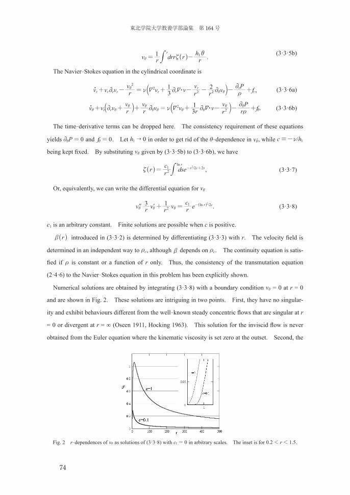
Numerical solutions are obtained by integrating (3·3·8) with a boundary condition vi = 0 at r = 0

and are shown in Fig. 2.　These solutions are intriguing in two points.　First, they have no singular-

ity and exhibit behaviours different from the well-known steady concentric flows that are singular at r

= 0 or divergent at r = ∞ (Oseen 1911, Hocking 1963).　This solution for the inviscid flow is never

obtained from the Euler equation where the kinematic viscosity is set zero at the outset.　Second, the

.v r drr r rh1 r1gi

= -i ^ h#

,v v v rv v v r

vr v P f3

1 2r r r r r r

r rr

22

2 2$2 2 22

U Uot

+ - = + - - - +ii io b l

.v v v rv

rv v v r v r

vrP f3

1r r

22$2 2 2

2U Uo

t+ + + = + - - +i i

i ii i i i

i iio a bk l

,r rc dse /

lns c s

r

21 2 22

g = - +^ h #

i .v r v r v rc e3 1 /ln r c

21 22+ =i i-m l ^ h

Fig. 2 r-dependences of vi as solutions of (3·3·8) with c 01= in arbitrary scales.　The inset is for . .r0 2 1 51 1 .

11

Fig.2 r-dependences of θv as solutions of (3·3·8) with c1 = 0 in arbitrary scales. The inset is for 0.2 < r < 1.5.

ii) Perturbation

The solution presented above has a flow profile quite similar to the ones used in the phenomenology of

typhoon, so that it may be of a matter of interest to inquire what kind of perturbation is allowed around the

solution. Let the radial and the azimuthal components are perturbed as r r r rδ δ→ + =v v v v , θ θ θδ→ +v v v .

Substituting these in (3·3·6a) and (3·3·6b) and linearlizing the equations in rδv and θδv , we have

2 rr

Pr

θ θδδ δρ

∂− = −

v vv , (3·3·9a)

1r r

Pr r rθ θ θ

θ θ θ θδ δ δ δρ

∂ + ∂ + + ∂ = −

v vv v v v , (3·3·9b)

where uses have been made of 0ν = , 0θ θ∂ =v and Pθ∂ = 0. These equations relate the variations in the

pressure, the density, rδv and θδv . Let us assume that the density variation and the resultant pressure

variation are small and the r.h.s. of each equation can be neglected. Then, the perturbations are expressed by

sinusoidal functions

0sin ( )A n t trθ

θδ θ = − −

vv , (3·3·10a)

02 2 cos ( ) ,t

rAdt n t t

r n rθ θ

θδ δ θ = = − − − ∫

v vv v (3·3·10b)

where n is an integer and designates the mode of oscillation. This expression is valid for large n limit (see

Appendix). rδv of high modes will be neglected. Various kinds of perturbations are observed by varying the

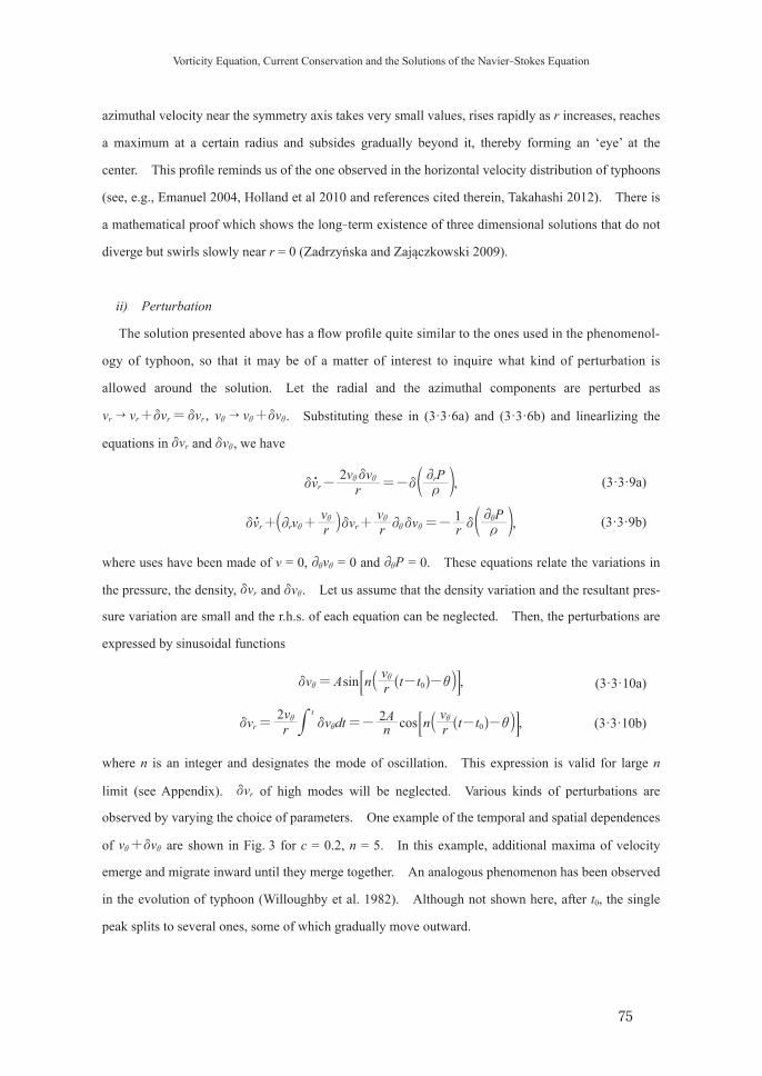
choice of parameters. One example of the temporal and spatial dependences of θ θδ+v v are shown in Fig.3

for c = 0.2, n=5. In this example, additional maxima of velocity emerge and migrate inward until they merge


75

azimuthal velocity near the symmetry axis takes very small values, rises rapidly as r increases, reaches

a maximum at a certain radius and subsides gradually beyond it, thereby forming an ‘eye’ at the

center.　This profile reminds us of the one observed in the horizontal velocity distribution of typhoons

(see, e.g., Emanuel 2004, Holland et al 2010 and references cited therein, Takahashi 2012).　There is

a mathematical proof which shows the long-term existence of three dimensional solutions that do not

diverge but swirls slowly near r = 0 (Zadrzyńska and Zajączkowski 2009).

ii)　Perturbation

The solution presented above has a flow profile quite similar to the ones used in the phenomenol-

ogy of typhoon, so that it may be of a matter of interest to inquire what kind of perturbation is

allowed around the solution.　Let the radial and the azimuthal components are perturbed as

,v v v v v v vr r r r" "d d d+ = +i i i.　Substituting these in (3·3·6a) and (3·3·6b) and linearlizing the

equations in vrd and vd i, we have

(3·3·9a)

(3·3·9b)

where uses have been made of v = 0, v2i i = 0 and P2i = 0.　These equations relate the variations in

the pressure, the density, vrd and vd i.　Let us assume that the density variation and the resultant pres-

sure variation are small and the r.h.s. of each equation can be neglected.　Then, the perturbations are

expressed by sinusoidal functions

(3·3·10a)

(3·3·10b)

where n is an integer and designates the mode of oscillation.　This expression is valid for large n

limit (see Appendix).　 vrd of high modes will be neglected.　Various kinds of perturbations are

observed by varying the choice of parameters.　One example of the temporal and spatial dependences

of v vd+i i are shown in Fig. 3 for c = 0.2, n = 5.　In this example, additional maxima of velocity

emerge and migrate inward until they merge together.　An analogous phenomenon has been observed

in the evolution of typhoon (Willoughby et al. 1982).　Although not shown here, after t0, the single

peak splits to several ones, some of which gradually move outward.

,v rv v P2

rr2d

ddt

- =-i io d n

,v v rv v r

v v rP1

r r r2 22

d d d dt

+ + + =-ii i

i iio a dk n

,sinv A n rv t t0d i= - -iiâ h k: D

,cosv rv v dt n

A n rv t t2 2

r

t

0d d i= =- - -ii

iâ h k: D#


76

iii)　Viscous fluid

The second solution describes a swirling inflow of a viscous and compressible fluid.　There, an

additional singularity emerges at r = 1.　Those singularities were avoided by placing a rotating

boundary with some radial distance.　The details on this solution will be reported elsewhere.　

Example 4 : Unsteady flow

In this example, a time-dependent solution corresponding to the superposition of the wave func-

tions is considered.　The simplest one may be a superposition of free plane waves :

(3·4·1)

Here we set N = 2 and assume 0k k1 2# ! and ja ’s are real.　By this specification of the wave func-

tion, the density and the phase are determined as

(3·4·2a)

(3·4·2b)

ct and d both are time-dependent.　Since

(3·4·3a)

(3·4·3b)

k, .e m2

k rj

i t i

j

N

jj

1

2j j= =a ~W $+

=

~-!

2 , 0,cos t k r k k kc 12

22

1 2 1 2 1 2$= + + = =!t a a a a ~ ~ ~ ~- - -^ h

k r.tan cos

sinttk rj j jj

j j jj

$

$d

a ~

a ~=

-

-

^

^

h

h

!!

2 sin tk k rc 1 2 $=Ut a a ~-^ h

, ,cos t1 k k K k r K k kc

121 2

22 1 2 1 2$= + + = +Ud

ta a a a ~- -^^ hh

Fig. 3 Temporal variation of the perturbed azimuthal velocity /sinv A n v r t t0 i+ - -i i^^ h h6 @ from t = 0 to 100 for c = 0.2, n=1, t0 = 100 and A = 0.05 at θ = 0.　vi is the solution to (3·3·8) with c1 = 1.

12

together. An analogous phenomenon has been observed in the evolution of typhoon (Willoughby et al. 1982).

Although not shown here, after t0, the single peak splits to several ones, some of which gradually move

outward.

Fig.3 Temporal variation of the perturbed azimuthal velocity [ ]0sin (( / )( ) )A n r t tθ θ θ+ − −v v from t = 0 to 100 for

c = 0.2, n=1, t0 = 100 and A=0.05 at θ = 0. θv is the solution to (3·3·8) with 1c = 1.

iii) Viscous fluid

The second solution describes a swirling inflow of a viscous and compressible fluid. There, an additional

singularity emerges at r=1. Those singularities were avoided by placing a rotating boundary with some radial

distance. The details on this solution will be reported elsewhere.

Example 4: Unsteady flow

In this example, a time-dependent solution corresponding to the superposition of the wave functions is

considered. The simplest one may be the superposition of free plane waves:

1

j jN i t i

jj

e ωψ α − + ⋅

== ∑ k r

，2

2j

j mω =

k. (3·4·1)

Here we set 2N = and assume 1 2 0× ≠k k and jα ’s are real. By this specification of the wave function,

the density and the phase are determined as

2 2c 1 2 1 22 cos( )tρ α α α α ω= + + − ⋅k r ， 1 2 1 20,ω ω ω= − ≠ = −k k k (3·4·2a)

sin( )tan

cos( )j j j j

j j j j

tt

α ωδ

α ω− ⋅

=− ⋅

∑∑

k rk r

. (3·4·2b)

cρ and δ both are time-dependent. Since


77

(2·4·6) is written as

(3·4·4)

We assumed that the r dependence of g emerges through ct .　In order for XzU to meet this condition,

Xz must have the form like

(3·4·5)

b is an arbitrary function of t k r$~- .　In particular, b is allowed to be complex.　This is possible

because (3·4·4) is linear in g.　Xz term gives a contribution in (3·4·4) only when q is not parallel to k.　

Noting that kc \Ut b^ h , we rewrite (3·4·4) as

(3·4·6)

Namely, g is an arbitrary function of t k r$~- .　If q = 0, the last term on the r.h.s. is absent and we

would have a simple time-dependent extension of Example 2.

By way of example, we here consider a case

(3·4·7a)

(3·4·7b)

where k, ω, V and c1 are constant.　Considering the arbitrariness of b, we allow these constants to be

complex number.　By choosing q=(－ky, kx, 0), the Navier-Stokes equation for the above v becomes

(3·4·8)

One of the reasonable assumptions for the density is that t varies as a function of t k r$~- .　In this

case, the continuity equation (2·1·3) leads to the dispersion relation

(3·4·9)

This means that the acceleration term of (2·1·1) identically vanishes and the viscous force, pressure

gradient and the external force must be balanced by themselves.　This condition is realized by

(3·4·10)

where, , P0 0t and c2 are constants.　f given in (3·4·10) is also constant.　As noted above, k and ω

can be complex and physical quantities are obtained by taking the real parts in (3·4·7) and (3·4·10).　

Specifically, when k and ω are pure imaginary, the solution is a uniform propagating sound wave in a

k K k k k rk

.ln ln sina tX

c

z z$

$$ $

#= +U U

Ug

oo ~

ot- -l ^^ hh

X q rz c $=ot b

2 .ln a t dk k kK k k r k

q k zt

1 22 2 2

k r$

$$

#U

a ao

go

~ pb p=- - -$~-

b ^ ^l h h#

, ,c e A c ek V rtz

t1 2

1k r k r $= = +g $ $~ ~- -

, ,vc k

e V v c k e Vk kxy t

y yx t

x21

21k r k r= + =- -$ $~ ~- -

.c

k V k V e c e Pkq

q fx y y xt t

21

1k r k r= +

U~ o

t- + - -$ $~ ~- -^ h

.k V k V 0x y y x~- + =

/ , , ,c c e P P c cq r f qt101

1 2 0 2 2 01k r $= + = =t t o t- -$ ~- - - -^ h


78

compressive fluid.　The ‘sound’ velocity is , ,V V 0c y xk$= =U ~ -^ h, where V has been assumed real.　

This is nothing but the average flow velocity.　Namely, there is no propagation in the rest frame of

the fluid.

If t is constant, it is possible to balance the pressure gradient term with the external force.　In this

case, it is easy to show, by assuming a general form t k r$g ~-^ h for g to determine Az, that the veloc-

ity field is given by

(3·4·11)

The continuity equation is satisfied without the constraint (3·4·9).　In particular, nontrivial solutions

are obtained even when V = 0.　The flow becomes the generalized Beltrami flow when 0k V z# = .　

The case of V = 0 has been studied by Taylor (1923), Kampe and Feriet (1930, 1932) and Wang

(1966).

4.　Two degrees of freedom

In the previous section, we assumed that g is a function of a single ct and treated the differential

equation in substantially one spatial dimension.　In other words, we considered the flows of essen-

tially one degree of freedom.

Owing to the linearity of (2·4·6) in g, the extension to the two degrees of freedom is, at least for-

mally, straightforward.　We adopt two sets of density and current which have independent coordinate

dependences.　Let the densities and phases be cjt and the phases , ,j 1 2jd = .　Although some com-

plexity emerges in (2·3·9) due to the coupling among cjt ’s, the equation will be simplified if one can

choose two cjt such that 0cj ck$U Ut t = for j k! .　In this case, (2·3·9) becomes a summation of the

contribution from each cjt and g will be expressed as c c1 1 2 2g g t g t= +^ ^h h.

We apply the above idea to the second example in the previous section.　Corresponding to two

orthogonal vectors, we may have two independent g’s, which obey the equations

(4·1)

The total g will be given by their sum as

(4·2)

The simplest stream function with no boundary may be

, .vc k

e V v c k e Vk k/ /

xy t

y yx t

x21

21k V k r k k V k r kz z

2 2= + = +# $ # $+ +~ ~ o ~ ~ o- - - -^ ^ ^ ^h h h h

21 ,ln ln ln lnak x ak y2 2x c y c

11

22= =2 2g

ot g

ot- - - -l l

.c e c ec x c y1 3

2 4g= +


79

(4·3)

The velocity field is given by

(4·4)

The continuity is satisfied for incompressible fluid.　The Navier-Stoke equation is

(4·5)

Comparing both sides, the consistent solution for the incompressible fluid is given by

(4·6)

This describes a flow ‘into a corner’ between semi-infinite planes having suction (Berker 1963).

5.　Summary

Focusing on the two-dimensional solenoidal flows, we derived a liner differential equation – the

transmutation equation – that relates the vorticity g to arbitrary conserved currents.　The stream func-

tion Az is obtained by solving Poisson’s equation with g as source function.　Any conserved currents

will be used as inputs to the transmutation equation to obtain numerical solutions.　

Some exact solutions are also obtained through the method, which shows the consistency of the

transmutation equation with the Navier-Stokes equation.　The integration constants that are intro-

duced in this procedure are, together with the density, the pressure and the external force, determined

from the requirement that the velocity field obeys the original Navier-Stokes equation and the conti-

nuity equation.　In this paper, this matching process was shown to be performed easily and consis-

tently.

The transmutation equation involves the Xz term that emerges when the combined equation of the

vorticity and continuity equations is integrated.　We saw that the familiar solutions were obtained in

case the Xz term was neglected.　When Xz term was pertinently taken into account, interesting new

solutions were found.　In particular, the solution for the inviscid concentric flow reproduces the pro-

file of the horizontal air flow of tropical cyclone or typhoon extremely well (Emanuel 2004, Holland

et al. 2010, Takahashi 2012).

.A cc e c

c e c x c yzc x c y

221

423

5 62 4=- - + +

, .v cc e c v c

c e cxc y

yc x

4

36

2

15

4 2= + =- -

,

.

v c e c c e P f

v c e c c eP

f

yc y c y x

x

xc x c x y

y

3 3 4

1 1 2

4 4

2 2

= +

= +

2

2

ot

ot

- - -

-

/ , .c c U c c U2 4 5 6o= =- =- =


80

Our method facilitates solving the Navier-Stoke equation for one degree of freedom, and will be

exploitable in two degrees of freedom, too.　Whether an extension to the three-dimension is possible

is an open question.

Acknowledgement

Thanks are due to Dr. Hoshino at Tohoku Gakuin University for his interesting comments on the

solutions of the Navier-Stokes equation.

Appendix

Here we show that, when the right hand sides of (3·3·9) are neglected, vrd is small as compared to

vd i for high modes.　Take the time derivative of (3·3·9b) and substitute (3·3·9a) to eliminate vrdo :

(A1)

where vi is a function of r only.　Substituting for vd i an ansatz

(A2)

where t0 is a constant, we have

(A3)

Here, primes on ψ stand for derivatives with respect to g r t t0/h i- -^ ^h h .　In order for (A3) to

have non-trivial solutions, the ratio of the coefficients of ψ and W m must be a constant, n2.　Then, (A3)

decomposes to two equations :

(A4)

(A5)

(A5) implies that hW^ h is a sinusoidal function of h,

(A6)

Since vd i is single-valued in i, n must be an integer.　

(A4) yields

,v rv v r

v v rv v2 0r2 2d d d+ + + =i

ii i

ii

iip o a k

v g r t t0=d iW - -i ^ ^_ h h i

0.g r rv g r r

v v rv2

r2 + + =2h hW W- i i

iim^ â ^ a ^h hk h k h

,g r rv g r n r

v v rv2 0r

22 2- + + =i i

ii^ ^ ah h k

0.n2+ =h hW Wm^ ^h h

or .sin cosn n= h hW


81

(A7)

For time-dependent solutions with high mode, /g r v r+ i^ h .　In this case, (3·3·9a) together with (A2)

and (3·3·9b) results in

(A8)

This proves the smallness of vr relative to vi for large n.　

References

Berker R 1963 Encyclopedia of Physics (ed. Flugge S) VIII/2 Springer (Berlin) 1.Couette M 1890 Ann. Chim. Phys. (6) 21 433.Drazin P and Riley N 2006 The Navier-Stokes Equations A Classification of Flows and Exact Solutions

Cambridge Univ. Press.Emanuel K A 2004 Atmospheric Turbulence and Mesoscale Meteorology, Federovich E et al (eds) Cam-

bridge Univ. Press.Hocking L M 1963 AIAA J. 1 1222.Holland G J, Belanger J I and Fritz A 2010 Mon. Wea. Rev. 138 4393.Kampe de Feriet J 1930 Proc. Int. Congr. Appl. Mech. 3rd Stockholm 334; 1932 Verh. Int. Math. Kongr.

Zurich 2 298.Navier C -L -M -H 1827 Mem. Acad. Sci. Inst. France (2) 6 389. Oseen C W 1911 Ark. Mat. Astron. Fys. 7 14.Poisson S -D 1831 J. Ec. Polytec. 13 cahier 20 1.Saint-Venant B 1843 C. R. Acad. Sci. Paris 17 1240.Stokes G G 1845 Trans. Cambridge Philos. Soc. 8 287.Takahashi K 2012 Talk at the workshop of Meteorological Society of Japan (Sendai).Taylor G I 1923 Phil. Mag. Ser 6, 46 671.Tsien H S 1943 Q. Appl. Math. I 130.Wang C Y 1966 J. Appl. Mech. 33 696.Wang C Y 1990 Acta Mech. 81 69; 1991 Annu. Rev. Fluid Mech. 70 351; 1991 Annu. Rev. Fluid Mech.

23 159.Willoughby H E, Clos J A and Shoreibah M G 1982 J. Atmos. Sci. 39 395.Zadrzyńska E and Zajączkowski W M 2009 J. Math. Fluid. Mech. 11 126.

i .g r rv

n rv

n rv v

21 1 8 8

22

2!= + +i i i l^ b ah l k< F

.cosv n n2r+d h-

Documents

Vorticity Equation, Current Conservation and the Solutions