Vortical and turbulent structures for KVLCC2 at drift ... · Vortical and turbulent structures for KVLCC2 at drift angle 0, 12, and 30 degrees Tao Xinga,n, Shanti Bhushanb, Frederick

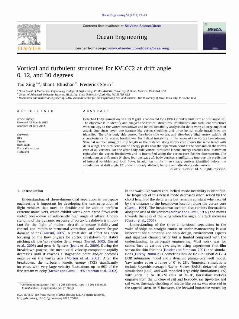
Ocean Engineering 55 (2012) 23–43

Contents lists available at SciVerse ScienceDirect

Ocean Engineering

0029-80

http://d

n Corr

E-m

journal homepage: www.elsevier.com/locate/oceaneng

Vortical and turbulent structures for KVLCC2 at drift angle0, 12, and 30 degrees

Tao Xing a,n, Shanti Bhushan b, Frederick Stern c

a Department of Mechanical Engineering, College of Engineering, PO Box 440902, University of Idaho, Moscow, ID 83844, USAb Center of Advanced Vehicular Systems, Mississippi State University, Starkville, MS 39759, USAc Mechanical and Industrial Engineering, 2416 Seamans Center for the Engineering Arts and Sciences, The University of Iowa, Iowa City, IA 52242, USA

a r t i c l e i n f o

Article history:

Received 12 March 2012

Accepted 21 July 2012

Keywords:

DES

Tanker

Drift angle

Vortical structure

Turbulent

18/$ - see front matter & 2012 Elsevier Ltd. A

x.doi.org/10.1016/j.oceaneng.2012.07.026

esponding author. Tel.: þ1 208 885 9032; fax

ail address: [email protected] (T. Xing).

a b s t r a c t

Detached Eddy Simulation on a 13 M grid is conducted for a KVLCC2 tanker hull form at drift angle 301.

The objective is to identify and analyze the vortical structures, instabilities, and turbulent structures

with analogy to the vortex breakdown and helical instability analysis for delta wing at large angles of

attack. One shear layer, one Karman-like vortex shedding, and three helical mode instabilities are

identified. The after-body side vortex, fore-body side vortex, and after-body bilge vortex exhibit all

characteristics for vortex breakdown. For helical instability in the wake of the vortex breakdowns,

Strouhal number using the ship length or the distance along vortex core shows the same trend with

delta wings. The turbulent kinetic energy peaks near the separation point at the bow and on the vortex

core of all vortices. For the after-body side vortex, turbulent kinetic energy reaches local maximum

right after the vortex breakdown and is intensified along the vortex core further downstream. The

simulations at drift angle 01 show four unsteady aft-body vortices, significantly improve the prediction

of integral variables and local flows. In addition to the three steady vortices identified before, the

simulations at drift angle 121 show unsteady aft-body hairpin and after-body side vortices.

& 2012 Elsevier Ltd. All rights reserved.

1. Introduction

Understanding of three-dimensional separation in aerospaceengineering is important for developing the next generation offlight vehicles that must be flexible and be able to performextreme maneuvers, which exhibit vortex-dominated flows withvortex breakdown at sufficiently high angle of attack. Under-standing of the dynamic response of vortex breakdown is impor-tant for the flight of modern aircraft to ensure stability andcontrol and minimize structural vibrations and severe fatiguedamage of fins (Gursul, 2005). A great deal of effort has beenfocusing on the flow physics for vortex breakdown for static/pitching slender/non-slender delta wings (Gursul, 2005; Gursulet al., 2005) and generic fighters (Jeans et al., 2009). During thebreakdown process, the mean axial velocity component rapidlydecreases until it reaches a stagnation point and/or becomesnegative on the vortex axis (Morton et al., 2002). After thebreakdown, the turbulent kinetic energy (TKE) significantlyincreases with very large velocity fluctuations up to 60% of thefree stream velocity (Menke and Gursul, 1997; Morton et al., 2002).

ll rights reserved.

: þ1 208 885 9031.

In the wake-like vortex core, helical mode instability is identified.The frequency of this helical mode decreases when scaled by thechord length of the delta wing but remains constant when scaledby the distance to the breakdown location along the vortex core(Gursul, 1994). The breakdown location also exhibits fluctuationsalong the axis of the vortices (Menke and Gursul, 1997) and movestowards the apex of the wing when the angle of attack increases(Gursul et al., 2005).

Understanding of the three-dimensional separation in thewake of ships on straight course or under maneuvering is alsoimportant for submarine and ship design, environment aspectsand signature characteristics but is limited compared with theunderstanding in aerospace engineering. Most work was forsubmarines at various yaw angles using experiment (hot-filmsensor for skin-friction) (Hosder and Simpson, 2001) and simula-tions (Fureby, 2008a,b). Geometries include DARPA Suboff AFF2, aDOR submarine model and a dynamic plunge-pitch-roll model.Yaw angles cover a range of 01 to 281. Numerical simulationsinclude Reynolds averaged Navier–Stokes (RANS), detached-eddysimulations (DES), and wall-modeled large eddy simulations (LES)with grids up to 10.3 M cells. At b¼01, horseshoe vorticesoriginate from the juncture of sail and forebody, sail tip-vortex andsail wake. Unsteady shedding of hairpin-like vortex was observed inthe tapered stern. As b increases, the leeward horseshoe vortex leg

www.elsevier.com/locate/oceaneng

www.elsevier.com/locate/oceaneng

dx.doi.org/10.1016/j.oceaneng.2012.07.026



mailto:[email protected]


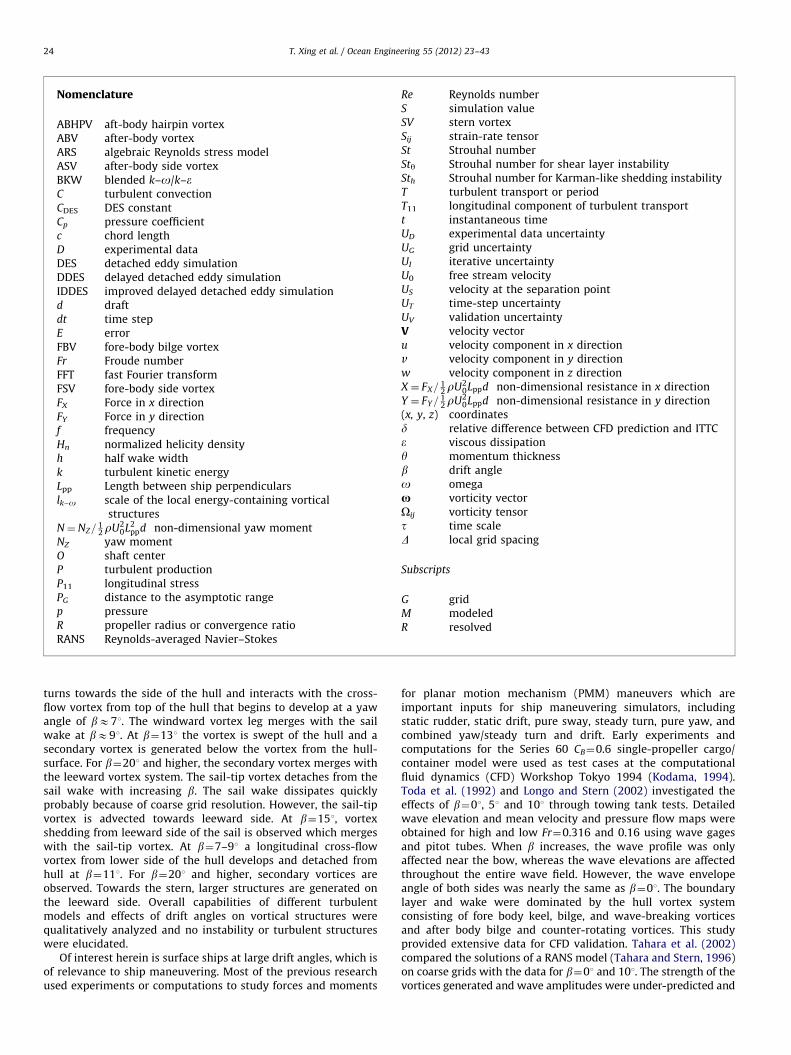
Nomenclature

ABHPV aft-body hairpin vortexABV after-body vortexARS algebraic Reynolds stress modelASV after-body side vortexBKW blended k–o/k–eC turbulent convectionCDES DES constantCp pressure coefficientc chord lengthD experimental dataDES detached eddy simulationDDES delayed detached eddy simulationIDDES improved delayed detached eddy simulationd draftdt time stepE errorFBV fore-body bilge vortexFr Froude numberFFT fast Fourier transformFSV fore-body side vortexFX Force in x directionFY Force in y directionf frequencyHn normalized helicity densityh half wake widthk turbulent kinetic energyLpp Length between ship perpendicularslk–o scale of the local energy-containing vortical

structuresN¼NZ=

12rU2

0L2ppd non-dimensional yaw moment

NZ yaw momentO shaft centerP turbulent productionP11 longitudinal stressPG distance to the asymptotic rangep pressureR propeller radius or convergence ratioRANS Reynolds-averaged Navier–Stokes

Re Reynolds numberS simulation valueSV stern vortexSij strain-rate tensorSt Strouhal numberSty Strouhal number for shear layer instabilitySth Strouhal number for Karman-like shedding instabilityT turbulent transport or periodT11 longitudinal component of turbulent transportt instantaneous timeUD experimental data uncertaintyUG grid uncertaintyUI iterative uncertaintyU0 free stream velocityUS velocity at the separation pointUT time-step uncertaintyUV validation uncertaintyV velocity vectoru velocity component in x directionv velocity component in y directionw velocity component in z directionX ¼ FX=

12rU2

0Lppd non-dimensional resistance in x directionY ¼ FY=

12rU2

0Lppd non-dimensional resistance in y direction(x, y, z) coordinatesd relative difference between CFD prediction and ITTCe viscous dissipationy momentum thicknessb drift angleo omegax vorticity vectorOij vorticity tensort time scaleD local grid spacing

Subscripts

G gridM modeledR resolved

T. Xing et al. / Ocean Engineering 55 (2012) 23–4324

turns towards the side of the hull and interacts with the cross-flow vortex from top of the hull that begins to develop at a yawangle of bE71. The windward vortex leg merges with the sailwake at bE91. At b¼131 the vortex is swept of the hull and asecondary vortex is generated below the vortex from the hull-surface. For b¼201 and higher, the secondary vortex merges withthe leeward vortex system. The sail-tip vortex detaches from thesail wake with increasing b. The sail wake dissipates quicklyprobably because of coarse grid resolution. However, the sail-tipvortex is advected towards leeward side. At b¼151, vortexshedding from leeward side of the sail is observed which mergeswith the sail-tip vortex. At b¼7–91 a longitudinal cross-flowvortex from lower side of the hull develops and detached fromhull at b¼111. For b¼201 and higher, secondary vortices areobserved. Towards the stern, larger structures are generated onthe leeward side. Overall capabilities of different turbulentmodels and effects of drift angles on vortical structures werequalitatively analyzed and no instability or turbulent structureswere elucidated.

Of interest herein is surface ships at large drift angles, which isof relevance to ship maneuvering. Most of the previous researchused experiments or computations to study forces and moments

for planar motion mechanism (PMM) maneuvers which areimportant inputs for ship maneuvering simulators, includingstatic rudder, static drift, pure sway, steady turn, pure yaw, andcombined yaw/steady turn and drift. Early experiments andcomputations for the Series 60 CB¼0.6 single-propeller cargo/container model were used as test cases at the computationalfluid dynamics (CFD) Workshop Tokyo 1994 (Kodama, 1994).Toda et al. (1992) and Longo and Stern (2002) investigated theeffects of b¼01, 51 and 101 through towing tank tests. Detailedwave elevation and mean velocity and pressure flow maps wereobtained for high and low Fr¼0.316 and 0.16 using wave gagesand pitot tubes. When b increases, the wave profile was onlyaffected near the bow, whereas the wave elevations are affectedthroughout the entire wave field. However, the wave envelopeangle of both sides was nearly the same as b¼01. The boundarylayer and wake were dominated by the hull vortex systemconsisting of fore body keel, bilge, and wave-breaking vorticesand after body bilge and counter-rotating vortices. This studyprovided extensive data for CFD validation. Tahara et al. (2002)compared the solutions of a RANS model (Tahara and Stern, 1996)on coarse grids with the data for b¼01 and 101. The strength of thevortices generated and wave amplitudes were under-predicted and

T. Xing et al. / Ocean Engineering 55 (2012) 23–43 25

the bow-wave system for the starboard side were not completelyreproduced in the global region. This was likely due to thedissipative nature of the RANS model and the insufficient resolu-tion of the grids. More recently, research focused on more modernhull forms such as the tanker (KVLCC2), container ship (KCS), andsurface combatant (5415) that were used as test cases for CFDWorkshops Gothenburg 2000, Tokyo 2005, SIMMAN 2008, andGothenburg 2010. KVLCC2 is of the most relevant to the currentstudy. In the CFD Workshop Gothenburg 2000, KVLCC2 test casefocused on turbulence modeling without free surface (windtunnel), whereas wave prediction was of interest for KCS and5415. Only straight ahead condition was investigated. Availabledata for validation include stern flow mean velocities, turbulence,surface pressure, and limiting streamlines for KVLCC2, and sternflow mean velocities without appendages and propellers, wavepattern/profile, and resistance for 5415. As summarized byLarsson et al. (2003), overall Reynolds stress RANS modelspredicted the best results than regular one- and zero-equationmodels and most two-equation models for KVLCC2. RANS modelsdid not predict the detailed hook-shape of the axial velocitycontour at the propeller plane that was thought to be created by abilge vortex. In the CFD Workshop Tokyo 2005, validation of CFDfor KVLCC2 at b¼01 used towing tank resistance and wind tunnellocal flow data including velocity and Reynolds stresses at thepropeller plane. The hook-shape was still not well captured.Towing tank measurement data for b¼121 were also collectedfor validation, including resistance and moment and one crosswake plane normal to the inflow for velocity contours and vectors(Kume et al., 2006). Overall the Reynolds-stress RANS modelpredicted the best results except for resistance at b¼121.Simonsen and Stern (2003) conducted rigorous verification andvalidation of a RANS code (CFDShip-Iowa-V.3) applied to amaneuvering problem for the tanker Esso Osaka covering the‘‘static rudder’’ and ‘‘pure drift’’ conditions up to 121. Fair resultsof forces and moments were obtained for the bare hull quantities,but larger deviations between experiment and computationswere observed for the forces and moments for the appended hull.The authors attributed this to the omission of the free surface andthe limitations of the blended k–e/k–o model. A later study by thesame authors (Simonsen and Stern, 2005) further characterizedthe flow pattern around the appended hull using the same codeand correlated behavior of the integral quantities with the flowfield. The flow pattern was characterized by fore and aft bodybilge and side vortices, which are similar for ‘‘straight-ahead’’ and‘‘static rudder’’ conditions, except in close vicinity of the rudder.The ‘‘pure drift’’ condition showed strong asymmetry on wind-ward vs. leeward sides and a more complex vortex system withadditional bilge vortices. For the considered drift and rudderangles, the friction was not particularly sensitive to the changedconditions, while more significant changes were observed forthe pressure. Also of relevance is the CFD/maneuvering simula-tion Workshop SIMMAN 2008 where comparisons were madebetween experiments and CFD for forces and yaw moment andhydrodynamic derivatives for KVLCC, KCS, 5415 in PMM condi-tions (Stern et al., 2011). Additionally, CFD were compared withthe stereo particle image velocimetry (PIV) measurements of axialvelocity contours, cross-flow vectors, and TKE in the nominal-wake plane for 5415. The static drift angle was up to 121. Allsimulations used RANS models except one simulation for KVLCCfor the free model test used DES model. The average number ofgrid points is 5.1 M. A third-order Taylor series Abkowitz-typemodel (Abkowitz, 1964) was used to evaluate the linear andnonlinear coefficients, i.e., hydrodynamic derivatives constructedusing CFD and experiments. For the test cases for all hulls, theerrors for forces, hydrodynamic derivatives, and reconstructionsaveraged over all submissions increase with the complexity of the

motion: X, Y, and N errors increased from 11%D to 19%D to 30%Dwhen going from static drift to pure sway to pure yaw. In general,X errors were larger than Y and N errors. Linear hydrodynamicderivative errors increased from 8%D to 23%D from pure swayto pure yaw. The errors for linear and nonlinear maneuveringderivatives averaged over all submissions were 6%D and 70%D,respectively. For the local flow quantities, the CFD by Sakamotoet al. (2008) agreed well with the IIHR stereo-PIV data (Yoon,2009) but with deficiencies of predicting momentum and turbu-lence at all the cross sections. This was attributed to the relativelycoarse grid and isotropic turbulence model applied sinceGuilmineau et al. (2008) predicted much better local flows usinga finer grid and an algebraic explicit algebraic stress k–o model(EASM). The results suggest that finer grids, more advancedturbulence and propeller models, and additional verification andvalidation (V&V) including local flow variables/measurements arerequired for improvements in the CFD predictions of static anddynamic PMM maneuvers. Additional post-workshop computa-tion by Sakamoto (2009) and experimental analysis by Yoon(2009) showed that multiple-run CFD or experiments curvefitting methods can provide better estimates for nonlinearmaneuvering derivatives than the single-run method used inthe CFD Workshop SIMMAN 2008, but statistical convergence ofthe higher-order Fourier series components is an issue. The CFD(Sakamoto, 2009) showed larger errors for larger b, i.e., E¼4.4%Dand 12.1%D for X for b¼101 and 201, respectively, and E¼

10–11%D for Y and 2%D for N for both b¼101 and 201.The turbulence model sensitivity study, which included URANSand DES, and grid refinements up to 20 M showed minimalimprovements.

Only recently, DES was applied to study surface ships at largedrift angles. As a precursory study of the current study, Xing et al.(2007) investigated the vortical structures and associatedinstabilities for KVLCC2 using a relative coarse grid with 1.6 Mpoints. It showed steady flows for b¼01 and 121 and unsteadyflow for b¼301 where vortical structures were identified andhelical instability was scaled using the theory of delta wings,which will be superseded by this study. Built on Xing et al. (2007),vortical structures and associated instabilities for an idealizedWigley hull for a wide range of b (101rbr601) are identified andextensively analyzed (Pinto-Heredero et al., 2010). The studyexamined b¼101, 301, 451, and 601 and the effect of Fr isevaluated at 101 and 601. Quantitative V&V were performed forb¼101; only quantitative verification is performed at b¼601 dueto the lack of experimental data. For unsteady cases (b¼451 andb¼601), Karman-like vortex shedding and tip vortices wereidentified and instabilities were analyzed. Analysis in this studywas limited and only qualitative since the finest grid only has1.4 M points. Ismail et al. (2010) used blended k–o/k–e based DESmodel and algebraic Reynolds Stress based DES (ARS–DES) modeland four convection schemes to study KVLCC2 at drift angle 0, 10,and 301 on grids up to 1.6 M. Overall, the ARS model improved thepredictions of resistance, axial velocity and turbulent quantitiesfor b¼01 when compared with the isotropic blended k–o/k––e(BKW) model. Coupling less dissipative convection schemes suchas 2nd order total variation diminishing with superbee limitation(TVD2S) and hybrid 2nd and 4th order (FD4h) with the BKWmodel produced very limited improvements in the forces andalmost no improvements in the local flow quantities at thenominal wake plane. Coupling the TVD2S scheme with ARS modelproduced remarkable improvements, in particular capturing thehook-shape for the axial velocity and TKE. The turbulent normaland shear stresses also show less dissipation, and are qualitativelyand quantitatively closer to the experimental data. For b¼121,however, local flow results produced by ARS and BKW turbulencemodels are almost identical. In fact, for this case the ARS


over-predicted the resistance, consistent with the findings ofTokyo CFD Workshop Tokyo 2005 (Hino, 2005). For b¼121,improvements of integral and the transported local quantitieswere observed when using the minimally dissipative TVD2Sscheme. These improvements were even more apparent forb¼301. Bhushan et al. (2011) conducted DES for 5415 bare hull201 static drift using three systematically refined grids consistingof 10 M, 148 M, and 250 M points. Grid verification study showsmostly converged solutions for the forces with relatively smallgrid uncertainties. However, divergence is obtained for themoment due to small grid changes with relatively large iterativeerrors. Compared to the large error in Sakamoto (2009) for b¼201,predictions of the forces and moments were significantlyimproved even on the coarse grid, which suggests that the largeerror was due to un-optimized grid design. Errors in externalforces in surge, sway, and yaw moment were reduced to less than5%D, which is comparable to errors for straight-ahead resistanceat the CFD Workshops Gothenburg 2000 and Tokyo 2005. Thisstudy also provided high resolution of vortical and turbulentstructures. Instabilities associated with the unsteady frequenciesfor forces and TKE budgets are pending analysis. In the mostrecent CFD Workshop Gothenburg 2010 (Larsson et al., 2011),KVLCC2, KCS, and 5415 were used to validate CFD simulations atb¼01. Also relevant to the current study is KVLCC2 where thesame wind tunnel data used in the CFD Workshop Tokyo 2005were used for validation. CFD used RANS, ARS, DES, and delayedDES (DDES) including the largest-scale computations using hun-dreds of millions grid points. Compared to CFD Workshop Tokyo2005 results, the standard deviation is substantially reduced from6.2%D to 1.2%D for the towed KVLCC2 in the fixed condition.9Emean9 is well below 2%D, although still not within the experi-mental accuracy. The details of the nominal wake of the tankerhull were predicted very well using anisotropic turbulencemodels for both mean velocity and turbulence. DES seemed toover-predict the anisotropy, thereby exaggerating the bilge vortexstrength and the hook-shape in the wake contours. More resultsfor this workshop will be discussed later.

The objective of this study is to identify and analyze thevortical structures, instabilities, and turbulent structures for theKVLCC2 tanker at b¼301 with analogy to the vortex breakdownand helical instability analysis for delta wing at large angles ofattack (Gursul, 1994). The approach is to apply ARS–DES on a finegrid to highly resolve TKE including simulations for b¼01 andb¼121 for evaluating the effect of b on the evolution of vorticalstructures. Verification is conducted for b¼01 and b¼301. Valida-tion is conducted for b¼01 and b¼121 using the same experi-mental data used in the previous CFD Workshops. For b¼01,additional DES and DDES simulations are conducted using a verylarge grid with 305 M points (Grid 0). The best solutions weresubmitted to the CFD Workshop Gothenburg 2010. Shear layerand Karman-like shedding instabilities will be analyzed followingXing et al. (2007) and Kandasamy et al. (2009). Turbulentstructures will be analyzed following Xing et al. (2007). The mostimportant results are presented herein and the complete resultsare presented in the supplemental materials for b¼01 and b¼301available upon request.

2. Computational method

The general-purpose solver CFDShip-Iowa-V.4 (Carrica et al.,2007) solves the unsteady RANS (URANS) or DES equations in theliquid phase of a free surface flow. The free surface is capturedusing a single-phase level set method and the turbulence ismodeled by isotropic or anisotropic turbulence models. Numericalmethods include advanced iterative solvers, second and higher

order finite difference schemes with conservative formulations,parallelization based on a domain decomposition approach usingthe message-passing interface (MPI), and dynamic overset gridsfor local grid refinement and large-amplitude motions.

2.1. Equations of motion and pressure Poisson equation

All governing equations are non-dimensionalized using thefree stream velocity U0, the ship length L, and the water density rand viscosity m. For Cartesian coordinates, the incompressiblecontinuity and momentum equations in nondimensional tensorform are:

@Ui

@xi¼ 0 ð1Þ

@Ui

@tþUj

@Ui

@xj¼�

@p

@xiþ

1

Re

@2Ui

@xj@xj�@

@xjuiuj ð2Þ

In order to accommodate complex geometries, generalized curvi-linear coordinates are used. The continuous governing Eqs. (1)and (2) are transformed from the physical domain in Cartesiancoordinates (x, y, z, t) into the computational domain in non-orthogonal curvilinear coordinates (x, Z, z, t) by applying thechain rule for partial derivatives, which results in continuity andmomentum equations given by Carrica et al. (2006):

1

J

@

@xjðbj

iUiÞ ¼ 0 ð3Þ

@Ui

@t þ1

Jbk

j Uj�@xj

@t

� �@Ui

@xk¼�

1

Jbk

i

@p

@xkþ

1

J

@

@xj

bjib

ki

JReef f

@Ui

@xk

!þ

bkj

J

@nt

@xk

bli

J

@Uj

@xlþSi

ð4Þ

The descretized momentum equations for any interior pointcan be written as:

Ui ¼�

PnbanbUi,nb�Si

aijk�

bki

Jaijk

@p

@xkð5Þ

The mass conservation Eq. (3) can be enforced using thediscretized form of the momentum Eq. (5) resulting in a Poissonequation for the pressure of the form (Carrica et al., 2006):

@

@xj

bjib

ki

Jaijk

@p

@xk

!¼

@

@xj

bji

aijk

Xnb

anbUi,nb�Si

!ð6Þ

2.2. Turbulence models

The ARS model (Wallin and Johansson, 2000) is based on amodified version of Menter’s k–e/k–o turbulence model as thescale determining model, and an explicit algebraic Reynolds stressmodel as the constitutive relation in place of the Boussinesqhypothesis:

uiuj ¼�nT@Ui

@xjþ@Uj

@xi

� �þ

2

3kdijþaðexÞ

ij k ð7Þ

The momentum equations remain the same with one addi-tional term @ðaðexÞ

ij kÞ=@xj included in the source to account for theeffect of the extra anisotropic tensor aðexÞ

ij :

aðexÞij ¼ b3 OikOkj�

1

3IIOdij

� �þb4ðSikOkj�OikSkjÞ

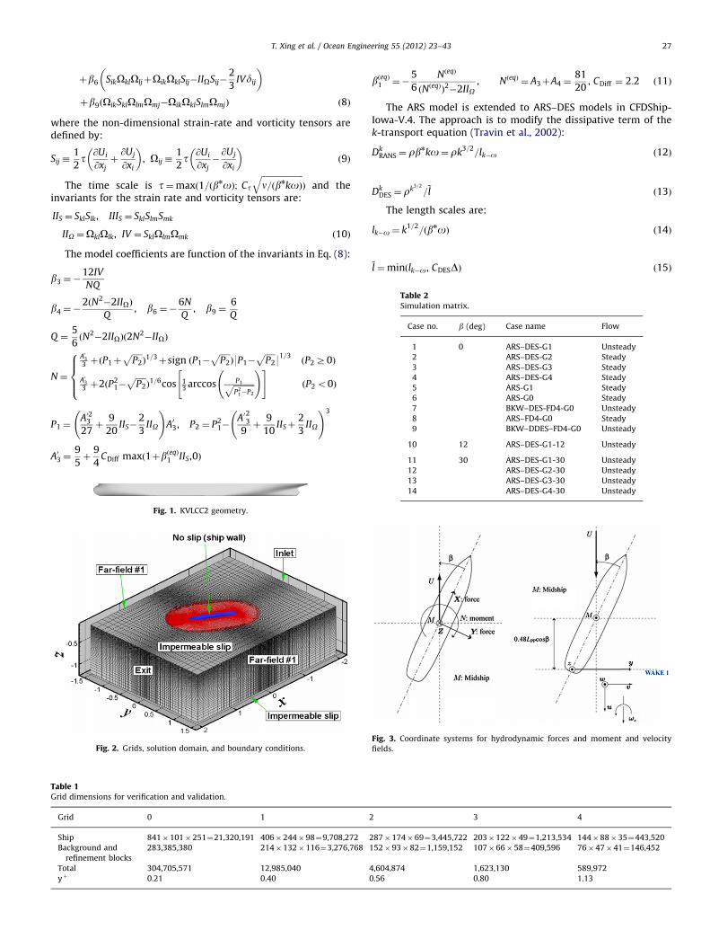
Table 2Simulation matrix.

Case no. b (deg) Case name Flow

1 0 ARS–DES-G1 Unsteady

2 ARS–DES-G2 Steady



5 ARS-G1 Steady

6 ARS-G0 Steady

7 BKW–DES-FD4-G0 Unsteady

8 ARS–FD4-G0 Steady

9 BKW–DDES–FD4-G0 Unsteady

10 12 ARS–DES-G1-12 Unsteady

11 30 ARS–DES-G1-30 Unsteady


þb6 SikOklOljþOikOklSlj�IIOSij�2

3IVdij

� �þb9ðOikSklOlmOmj�OikOklSlmOmjÞ ð8Þ

where the non-dimensional strain-rate and vorticity tensors aredefined by:

Sij �1

2t @Ui

@xjþ@Uj

@xi

� �, Oij �

1

2t @Ui

@xj�@Uj

@xi

� �ð9Þ

The time scale is t¼maxð1=ðbnoÞ; Ct

ffiffiffiffiffiffiffiffiffiffiffiffiffiffiffiffiffiffiffiffin=ðbnkoÞ

qÞ and the

invariants for the strain rate and vorticity tensors are:

IIS ¼ SklSlk, IIIS ¼ SklSlmSmk

IIO ¼OklOlk, IV ¼ SklOlmOmk ð10Þ

The model coefficients are function of the invariants in Eq. (8):

b3 ¼�12IV

NQ

b4 ¼�2ðN2�2IIOÞ

Q, b6 ¼�

6N

Q, b9 ¼

6

Q

Q ¼5

6ðN2�2IIOÞð2N2

�IIOÞ

N¼

A033 þðP1þ

ffiffiffiffiffiP2

pÞ1=3þsign ðP1�

ffiffiffiffiffiP2

pÞ9P1�

ffiffiffiffiffiP2

p91=3

ðP2Z0Þ

A033 þ2ðP2

1�ffiffiffiffiffiP2

pÞ1=6cos 1

3 arccos P1ffiffiffiffiffiffiffiffiffiffiP2

1�P2

p !" #ðP2o0Þ

8>><>>:

P1 ¼A02327þ

9

20IIS�

2

3IIO

!A03, P2 ¼ P2

1�A0

23

9þ

9

10IISþ

2

3IIO

!3

A03 ¼9

5þ

9

4CDiff maxð1þbðeqÞ

1 IIS,0Þ

Table 1Grid dimensions for verification and validation.

Grid 0 1

Ship 841�101�251¼21,320,191 406�244�98¼9,708,272

Background and

refinement blocks

283,385,380 214�132�116¼3,276,768

Total 304,705,571 12,985,040

yþ 0.21 0.40

Fig. 1. KVLCC2 geometry.

Fig. 2. Grids, solution domain, and boundary conditions.

bðeqÞ1 ¼�

5

6

NðeqÞ

ðNðeqÞÞ2�2IIO

, NðeqÞ¼ A3þA4 ¼

81

20, CDiff ¼ 2:2 ð11Þ

The ARS model is extended to ARS–DES models in CFDShip-Iowa-V.4. The approach is to modify the dissipative term of thek-transport equation (Travin et al., 2002):

DkRANS ¼ rb

nko¼ rk3=2=lk�o ð12Þ

DkDES ¼ r

k3=2

=~l ð13Þ

The length scales are:

lk�o ¼ k1=2=ðbnoÞ ð14Þ

~l ¼minðlk�o, CDESDÞ ð15Þ

2 3 4

287�174�69¼3,445,722 203�122�49¼1,213,534 144�88�35¼443,520

152�93�82¼1,159,152 107�66�58¼409,596 76�47�41¼146,452

4,604,874 1,623,130 589,972

0.56 0.80 1.13

12 ARS–DES-G2-30 Unsteady



Fig. 3. Coordinate systems for hydrodynamic forces and moment and velocity

fields.


where CDES is the DES constant, set at 0.65, the typical valuefor homogeneous turbulence, and D is the local grid spacing.Through this formulation, it is theoretically determined where theLES or the URANS will be applied. The length scale, lk–o, reflectsthe scale of the local energy-containing vortical structures. Insidethe boundary layer of a wall or inside a region where noseparation occurs, lk–o is small since TKE is small. Hence,~l ¼ lk�o and the URANS is used. When the flow separates, vorticesgenerate a significant increase of the TKE and lk–o, and the LES isused (~l ¼ CDESD). The ARS–DES model has been validated by thesimulation of a NACA0012 aerofoil at 601 angle of attack underthe same conditions as the study by Shur et al. (1999).

2.3. Numerical methods and high performance computing

The resulting algebraic systems for the variables, u, v, w, p, k,and o are solved in a sequential form and iterated to achieveconvergence within each time step. The equations are discretized

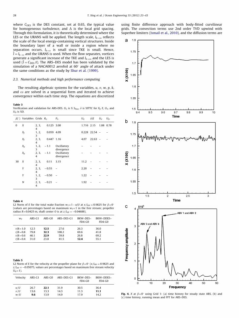
Table 5

L2 Norm of E for the velocity at the propeller plane for b¼01 (x=LPP ¼ 0:9825 and

z=LPP ¼�0:05075, values are percentages based on maximum free stream velocity

U0¼1).

Velocity ARS-G1 ARS-G0 ARS–DES-G1 BKW–DES–

FD4-G0

BKW–DDES–

FD4-G0

u=U 26.7 22.1 31.9 30.5 36.4

v=U 13.6 13.3 14.3 11.3 11.1w=U 9.6 13.9 14.9 17.9 14.2

Table 4

L2 Norm of E for the total wake fraction wT¼1�u/U at x=LPP ¼ 0:9825 for b¼01

(values are percentages based on maximum wT¼1 in the free stream; propeller

radius R¼0.0425 m, shaft center O is at z=LPP ¼�0:04688).

wT ARS-G1 ARS-G0 ARS–DES-G1 BKW–DES–

FD4-G0

BKW–DDES–

FD4-G0

r/R¼1.0 12.5 12.5 27.6 26.3 36.0

r/R¼0.8 79.8 32.3 108.2 69.6 41.8

r/R¼0.6 46.1 22.9 59.8 26.8 69.2

r/R¼0.4 31.0 23.8 41.5 12.4 55.1

Table 3

Verification and validation for ARS-DES. UG is % Sfine, d is %ITTC for Xf, E, UV, and

UD is %D.

b(1) Variables Grids RG PG UG d/E UV UD

0 X 2, 3,

4

0.125 3.00 1.716 2.15 1.88 0.78

Xf 1, 2,

3

0.059 4.09 0.228 22.54 – –

Xf 2, 3,

4

0.447 1.16 4.07 22.63 – –

Xp 1, 2,

3

�1.1 Oscillatory

divergence

– – –

Xp 2, 3,

4

�1.1 Oscillatory

divergence

– – – –

30 X 2, 3,

4

0.11 3.15 11.2 – – –

Y 2, 3,

4

�0.55 – 2.20 – – –

Y 1, 2,

3

�0.50 – 1.22 – – –

N 2, 3,

4

�0.21 – 1.92 – – –

using finite difference approach with body-fitted curvilineargrids. The convection terms use 2nd order TVD upwind withSuperbee limiters (Ismail et al., 2010), and the diffusion terms are

Fig. 4. X at b¼01 using Grid 1: (a) time history for steady state ARS, (b) and

(c) time history, running mean and FFT for ARS–DES.

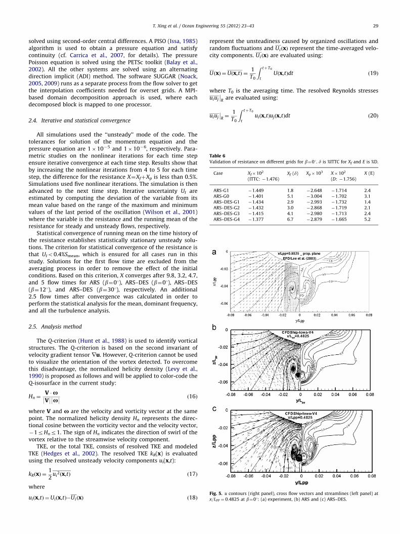
Fig. 5. u contours (right panel), cross flow vectors and streamlines (left panel) at

x=LPP ¼ 0:4825 at b¼01: (a) experiment, (b) ARS and (c) ARS–DES.

Table 6

Validation of resistance on different grids for b¼01. d is %ITTC for Xf and E is %D.

Case Xf�102

(ITTC: �1.476)Xf (d) Xp�103 X�102

(D: �1.756)

X (E)

ARS-G1 �1.449 1.8 �2.648 �1.714 2.4

ARS-G0 �1.401 5.1 �3.004 �1.702 3.1

ARS–DES-G1 �1.434 2.9 �2.993 �1.732 1.4

ARS–DES-G2 �1.432 3.0 �2.868 �1.719 2.1

ARS–DES-G3 �1.415 4.1 �2.980 �1.713 2.4

ARS–DES-G4 �1.377 6.7 �2.879 �1.665 5.2


solved using second-order central differences. A PISO (Issa, 1985)algorithm is used to obtain a pressure equation and satisfycontinuity (cf. Carrica et al., 2007, for details). The pressurePoisson equation is solved using the PETSc toolkit (Balay et al.,2002). All the other systems are solved using an alternatingdirection implicit (ADI) method. The software SUGGAR (Noack,2005, 2009) runs as a separate process from the flow solver to getthe interpolation coefficients needed for overset grids. A MPI-based domain decomposition approach is used, where eachdecomposed block is mapped to one processor.

2.4. Iterative and statistical convergence

All simulations used the ‘‘unsteady’’ mode of the code. Thetolerances for solution of the momentum equation and thepressure equation are 1�10�5 and 1�10�6, respectively. Para-metric studies on the nonlinear iterations for each time stepensure iterative convergence at each time step. Results show thatby increasing the nonlinear iterations from 4 to 5 for each timestep, the difference for the resistance X¼XfþXp is less than 0.5%.Simulations used five nonlinear iterations. The simulation is thenadvanced to the next time step. Iterative uncertainty UI areestimated by computing the deviation of the variable from itsmean value based on the range of the maximum and minimumvalues of the last period of the oscillation (Wilson et al., 2001)where the variable is the resistance and the running mean of theresistance for steady and unsteady flows, respectively.

Statistical convergence of running mean on the time history ofthe resistance establishes statistically stationary unsteady solu-tions. The criterion for statistical convergence of the resistance isthat UIo0.4%Smean, which is ensured for all cases run in thisstudy. Solutions for the first flow time are excluded from theaveraging process in order to remove the effect of the initialconditions. Based on this criterion, X converges after 9.8, 3.2, 4.7,and 5 flow times for ARS (b¼01), ARS–DES (b¼01), ARS–DES(b¼121), and ARS–DES (b¼301), respectively. An additional2.5 flow times after convergence was calculated in order toperform the statistical analysis for the mean, dominant frequency,and all the turbulence analysis.

2.5. Analysis method

The Q-criterion (Hunt et al., 1988) is used to identify vorticalstructures. The Q-criterion is based on the second invariant ofvelocity gradient tensor ru. However, Q-criterion cannot be usedto visualize the orientation of the vortex detected. To overcomethis disadvantage, the normalized helicity density (Levy et al.,1990) is proposed as follows and will be applied to color-code theQ-isosurface in the current study:

Hn ¼V �x9V99x9

ð16Þ

where V and x are the velocity and vorticity vector at the samepoint. The normalized helicity density Hn represents the direc-tional cosine between the vorticity vector and the velocity vector,�1rHnr1. The sign of Hn indicates the direction of swirl of thevortex relative to the streamwise velocity component.

TKE, or the total TKE, consists of resolved TKE and modeledTKE (Hedges et al., 2002). The resolved TKE kR(x) is evaluatedusing the resolved unsteady velocity components ui(x,t):

kRðxÞ ¼1

2ui

2ðx,tÞ ð17Þ

where

uiðx,tÞ ¼Uiðx,tÞ�Ui ðxÞ ð18Þ

represent the unsteadiness caused by organized oscillations andrandom fluctuations and Ui ðxÞ represent the time-averaged velo-city components. Ui ðxÞ are evaluated using:

UðxÞ ¼Uðx,tÞ ¼1

T0

Z tþT0

tUðx,tÞdt ð19Þ

where T0 is the averaging time. The resolved Reynolds stressesuiuj

��R

are evaluated using:

uiuj

��R¼

1

T0

Z tþT0

tuiðx,tÞujðx,tÞdt ð20Þ

Fig. 7. Instantaneous vortical structures (isosurface of Q¼300 colored by helicity) at b¼01: (a) ARS top view, (b) ARS bottom view, (c) ARS–DES top view and (d) ARS–DES

bottom view.

Fig. 6. Turbulent Kinetic energy contours at (x=LPP ¼ 0:4825) at b¼01: (a) experiment, (b) ARS and (c) ARS–DES.



The resolved TKE budget is evaluated using the time-averagedexact TKE transport equation (Le et al., 1997):

0¼�Uj@kR

@xj|fflfflfflfflffl{zfflfflfflfflffl}C

�uiuj

��R

@Ui

@xj|fflfflfflfflfflfflfflffl{zfflfflfflfflfflfflfflffl}P

�1

Re

@ui

@xk

@ui

@xk|fflfflfflfflfflfflfflfflffl{zfflfflfflfflfflfflfflfflffl}e

þ@

@xj

1

Re

@kR

@xj

� �|fflfflfflfflfflfflfflfflfflffl{zfflfflfflfflfflfflfflfflfflffl}

D

�1

2

@uiuiuj

@xj|fflfflfflfflfflfflfflffl{zfflfflfflfflfflfflfflffl}T

�@p0uj

@xj|fflfflffl{zfflfflffl}PT

ð21Þ

where the right hand side terms of the equation are, from the leftto right, turbulent convection (C), turbulent production (P),viscous dissipation (e), viscous diffusion (D), turbulent transport(T), and pressure transport (PT). These terms are evaluatedsimilarly to Ui ðxÞ (Eq. (19)) and p

0

(x,t) is defined similarly asui(x,t) (Eq.(18)). The resolved e cannot be evaluated since viscousdissipation occurs at the Kolmogorov scale and requires a directnumerical simulation grid, which is unaffordable for such a highRe flow. The time-averaged modeled TKE kMðxÞ is calculated bytime-averaging the kM(x,t) evaluated by the two-equation turbu-lence model. The modeled TKE budget terms are evaluated usingthe averaged modeled k equation:

0¼�Uj@kM

@xj|fflfflfflfflffl{zfflfflfflfflffl}C

�uiuj

��M

@Ui

@xj|fflfflfflfflfflfflfflfflffl{zfflfflfflfflfflfflfflfflffl}P

�bnkMo|fflfflfflfflfflffl{zfflfflfflfflfflffl}e

þ@

@xj

1

Re

@kM

@xj


D

þ@

@xj

nT

2

@kM

@xj


TþPT

ð22Þ

and the modeled Reynolds stresses are output at each time stepusing Eq. (7). As discussed early, T0 is chosen to be 2.5 flow times.Both resolved and modeled viscous diffusion terms are negligibledue to the very high Re. For completeness, the resolved TKE andTKE budget at b¼301 will be presented with exception for viscousdissipation (modeled). The total turbulent statistics comply pri-marily with the resolved and are not shown.

The overall procedure for V&V follows Stern et al. (2006).Verification is a process for assessing simulation numericaluncertainty USN, which is composed of iterative UI, grid UG, andtime-step UT uncertainties

U2SN ¼U2

I þU2GþU2

T ð23Þ

where estimation of UI follows section 2.4 and estimations forUG and UT follow the factor of safety (FS) method by Xing and Stern(2010). The purpose of validation is to assess interval of modelinguncertainty and thereby ascertain usefulness of modeling approach.The validation procedure follows Coleman and Stern (1997).The comparison error E is defined by the difference between thedata D and simulation S values

E¼D�S ð24Þ

and the validation uncertainty is defined as

UV ¼

ffiffiffiffiffiffiffiffiffiffiffiffiffiffiffiffiffiffiffiU2

SNþU2D

qð25Þ

where UD is the uncertainty of the experimental data. If 9E9oUV,the combination of all the errors in D and S is smaller than UV andvalidation is achieved at the UV interval.

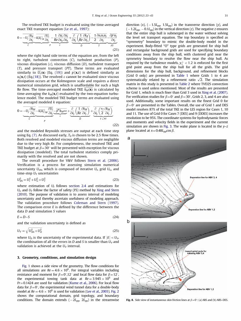
Fig. 8. Side view of instantaneous skin friction lines at b¼01: (a) ARS and (b) ARS–DES.

3. Geometry, conditions, and simulation design

Fig. 1 shows a side view of the geometry. The flow conditions forall simulations are Re¼ 4:6� 106. For integral variables includingresistance and moment for b¼01,121 and local flow data for b¼121,the experimental towing tank data at Re¼ 3:945� 106 andFr¼0.1424 are used for validation (Kume et al., 2006). For local flowdata for b¼01, the experimental wind tunnel data for a double-bodymodel at Re¼ 4:6� 106 is used for validation (Lee et al., 2003). Fig. 2shows the computational domain, grid topology, and boundaryconditions. The domain extends (�2Lpp, 2Lpp) in the streamwise

direction (x), (�1.5Lpp, 1.5Lpp) in the transverse direction (y), and(�1.2Lpp, �0.1Lpp) in the vertical direction (z). The negative z ensuresthat the entire ship hull is submerged in the water without solvingthe level set transport equation. The top boundary is specified as‘‘symmetry’’ boundary to mimic the double-body model in theexperiment. Body-fitted ‘‘O’’ type grids are generated for ship hulland rectangular background grids are used for specifying boundaryconditions away from the ship hull, with clustered grid near thesymmetry boundary to resolve the flow near the ship hull. Asrequired by the turbulence models, yþ1 o1:2 is enforced for the firstgrid point away from the ship hull for all the grids. The griddimensions for the ship hull, background, and refinement blocks(Grid 0 only) are presented in Table 1 where Grids 1 to 4 aresystematically related by a refinement ratio

ffiffiffi2p

. The simulationmatrix in this study is presented in Table 2 where TVD2S convectionscheme is used unless mentioned. Most of the results are presentedfor Grid 1, which is much finer than Grid 3 used in Xing et al. (2007).For verification studies for b¼01 and b¼301, Grids 2, 3, and 4 are alsoused. Additionally, some important results on the finest Grid 0 forb¼01 are presented in the Tables. Overall, the use of Grid 1 and DESmodel resolves 87% of the total TKE in the LES region for Cases 1, 10and 11. The use of Grid 0 for Cases 7 (DES) and 9 (DDES) increases theresolution to be 95%. The coordinate systems for hydrodynamic forcesand moments and velocity fields in the experiment and the currentsimulation are shown in Fig. 3. The wake plane is located in the y–z

plane located at x¼0.48Lppcosb.

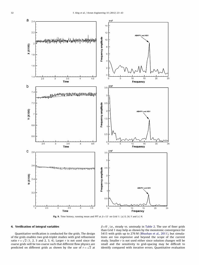
Fig. 9. Time history, running mean and FFT at b¼121 on Grid 1: (a) X, (b) Y and (c) N.


4. Verification of integral variables

Quantitative verification is conducted for the grids. The designof the grids enables two grid-triplet studies with grid refinementratio r¼

ffiffiffi2p

(1, 2, 3 and 2, 3, 4). Larger r is not used since thecoarse grids will be too coarse such that different flow physics arepredicted on different grids as shown by the use of r¼

ffiffiffi2p

at

b¼01, i.e., steady vs. unsteady in Table 2. The use of finer gridsthan Grid 1 may help as shown by the monotonic convergence for5415 with grids up to 276 M (Bhushan et al., 2011), but simula-tions are too expensive and beyond the scope of the currentstudy. Smaller r is not used either since solution changes will besmall and the sensitivity to grid-spacing may be difficult toidentify compared with iterative errors. Quantitative evaluation

Fig. 10. Nominal wake velocity vector plot at b¼121: (a) experiment and (b) ARS–DES.

Table 7

Validation of resistance for KVLCC2 for b¼121. E is %D.

Grid X�102

(D: �1.750)

X (E) Y�102

(D: 7.082)

Y (E) N�102

(D: 2.539)

N (E)

1 �2.047 16.97 7.358 3.90% 2.552 0.51


for time-step was not possible since large time-step leads tounstable solutions for ARS–DES on Grid 1 at b¼01, 121, and 301and simulations using smaller time-step are too expensive. None-theless, the current time-step (dt¼0.002) is only a 20% of thetypically dt for CFD simulations in ship hydrodynamics and it issufficiently small to resolve all the unsteadiness of the vorticalstructures and turbulent structures.

Previous simulation using ARS–DES on Grid 3 showed thatflow at b¼01 for KVLCC2 is steady and thus BKW or ARS modelwas used Xing et al. (2007). On Grid 1, ARS shows steady flow,whereas ARS–DES predicts unsteady flow. Table 3 shows V&V forthe resistance. For b¼01, monotonic convergence is only achievedon (2, 3, 4) for X and on (2, 3, 4) and (1, 2, 3) for Xf. The estimatedorders of accuracy show large oscillations as PG has values from1.16 to 4.09. Xp shows oscillatory divergence on the two gridtriplets. For b¼301, monotonic convergence is only achieved for X

on (2, 3, 4) with a large grid uncertainty. Oscillatory convergenceis achieved for Y on (1, 2, 3) and (2, 3, 4) and for N on (2, 3, 4) withmuch smaller grid uncertainties.

Overall the solutions are not in the asymptotic range, whichwas attributed to several reasons. At b¼01, ARS–DES on Grid 1 showsunsteady flow, whereas all other grids predict steady flows and thusthey are resolving different flow physics. Further refinement of thegrids may help but subject to the problem of separating iterativeerrors and grid solution changes on fine grids. Furthermore, gridrefinement for DES changes the numerical errors and the sub-gridscaling modeling errors simultaneously, which was not consideredfor all available solution verification methods. It should be also notedthat all grid-triplet studies except Xf for (2, 3, 4) estimate PG42,which cause unreasonably small uncertainties due to a small errorestimate. Recently, an alternative form of the FS method (FS1

method) was developed and evaluated using the same dataset asthe FS method by using pth instead of pRE in the error estimate forPG41 (Xing and Stern, 2011). FS1 method is more conservative thanthe FS method for PG42 and the use of FS1 method will increase UG

from 1.716%Sfine to 19.485%Sfine and thus UV from 1.88%D to 19.5%D.However, since the dataset to derive/validate the FS and FS1 methodsis restricted to PGo2, the pros/cons of using the FS or FS1 methodcannot be validated.

Fig. 11. Nominal wake velocity U at b¼121: (a) experiment and (b) ARS–DES.

5. Validation and analysis for b¼01

Cases 1–9 in Table 2 are for b¼01. Cases 1–4 are used forsolution verification for ARS–DES as previously discussed. Case5 is ARS on Grid 1. Cases 6–9 are for a much finer grid G0 withdifferent turbulence models (ARS, DES, DDES) and convectionschemes (FD4, TVD2S). Comparisons between cases 5 and 6 andbetween cases 1 and 7 show the effect of grids on ARS and DESmodel, respectively, where ARS shows less dependence on gridsthan ARS–DES. Cases 6 and 8 are used to evaluate the effect ofnumerical schemes on ARS model on Grid 0. It is found that theeffect of the two numerical schemes on results is negligible onsuch a fine grid. Effect of turbulence models on Grid 0 is evaluatedby comparing ARS and DES (cases 7 and 8) and DES and DDES(cases 7 and 9). Compared to ARS, ARS–DES improves theresistance and velocity prediction at the propeller plane; how-ever, ARS–DES tends to over-predict the velocity near the

symmetry plane and the Reynolds stresses at the propeller plane.The grid induced separation using ARS–DES model on G0 isresolved by BKW–DDES–FD4-G0 model, but both show modeledstress depletion inside the boundary layer, which suggest theneed to implement the improved DDES (IDDES) model.

Tables 4 and 5 show the L2 norm of the E of total wake fractionand velocity at the propeller plane for Cases 1, 5, 6, 7, 9. Theminimum value for E in each row is shown in bold face. None ofthe methods is consistently better than any other method. Over-all, ARS-G0 and ARS–DES-G1 were the best RANS and DES results,respectively, which were submitted to the CFD WorkshopGothenburg 2010 (Larsson et al., 2011). The present results forintegral variables and local flows are as good as the best CFDsolutions in that workshop.

The time history, running mean, and fast Fourier transform(FFT) for X on Grid 1 are shown in Fig. 4. ARS shows steady flow asshown in Fig. 4a by the converged constant X. ARS–DES showsunsteady flow as shown in Fig. 4b. For ARS–DES at b¼01, validationfor X is not achieved on grids (2,3,4) as E4UV (Table 3). This is dueto the very small UG and UD. If the FS1 method is used to estimate UG

then validation is achieved. Although the solutions are not in the


asymptotic range, E between the running mean and experimentaldata are less than 5%D except for the coarsest Grid 4 (Table 6).Grid 4 also causes that the validation on grid triplet (2, 3, 4) is notachieved. Table 6 also compares the predicted frictional resistance Xf

with ITTC 1957 and the total resistance X with the experimentaldata on different grids. As the grids are refined from 4 to 1, ddecrease from more than 6%ITTC to less than 3%ITTC for Xf and E

decreases from more than 5%D to less than 2%D for X. By excludingGrid 4, the averaged d and E are 3.3%ITTC and 2.8%D for Xf and X,respectively. It should be noted that the experimental data for X usedherein is based on the towing tank measurement without a rudder(Kume et al., 2006). The experimental data for X used for CFDWorkshop Gothenburg 2010 was based on the towing tank measure-ment with a rudder (Kim et al., 2001). If either one of the twoexperimental data is converted to be the same definition as the

Table 8Different instabilities and scaling at three different drift angles.

b (deg) Vortex name Location In

0 (ARS) ABV 1 (steady) Port –

ABV 2 (steady) Starboard –

ABV 3 (steady) Port –

ABV 4 (steady) Starboard –

0 (ARS–DES) ABV 1 Port 18

ABV 2 Starboard 18

ABV 3 Port 6.

ABV 4 Starboard 6.

12 (ARS–DES) ABV (steady) Leeward –

ABHPV (unsteady) Leeward 16

ASV (unsteady) Leeward 19

FBV (steady) Leeward –

FSV (steady) Leeward –

30 (ARS–DES) ABV Leeward Fi

ASV Windward Fi

FBV Leeward –

FSV Leeward Fi

ABHPV Leeward 31

Kelvin–Helmoholtz Leeward 38

Karman-like Leeward 17

SV (steady) Leeward –

Fig. 12. Vortex systems around the ship hull at b¼121 (isosurface of Q¼100

colored by helicity): (a) bottom view and (b) zoom in near the stern.

other, the difference between them is about 3.5%D. This suggests thatthe accuracy of the experimental data or the interaction between thehull and rudder is an issue, which is under investigation.

Fig. 5 shows the comparison of the experimental data andCFD on Grid 1 for averaged axial velocity at the propeller plane.The experiment clearly shows hook-shape pattern of the axialvelocity. As explained by Larsson et al. (2011) in the CFD Work-shop Gothenburg 2010, this pattern was caused by an intensestern bilge vortex and a secondary counter-rotating vortex closeto the vertical plane of symmetry. The secondary vortex cannot beseen clearly in the experiment due to limitation of the resolution.ARS under-estimates the size of the main vortex and predictssteady flow. ARS–DES shows significant improvements on esti-mating the size of the main vortex and prediction of the hook-shape pattern. Fig. 6 shows the total TKE, which shows the similartrend as that for axial velocity distributions, but with the peakvalue of TKE (�2.1%U0

2) over-predicted by 35%.Fig. 7 shows the instantaneous top and bottom views of the

vortical structures for ARS and ARS–DES. Both models clearly exhibitfour after-body vortices ABV1-4 with two on each side. The twovortices on the same side and the two vortices with symmetric tothe vertical symmetry plane are counter-rotating. However, the fourvortices are steady and unsteady for ARS and ARS–DES simulations,respectively. Additionally, ABV 3 and 4 are much longer than ABV1 and 2 for ARS, whereas the opposite is exhibited for ARS–DES.

Skin friction lines for ARS and ARS–DES are shown in Fig. 8a andFig. 8b, respectively, which clearly show the initiation of the vortices.For ARS, the four vortices are formed by the separation on the hubwhere ABV 3,4 and ABV 1,2 are initiated by the upper and lowersections of the separation line, respectively. For ARS–DES, theseparation line on the hub becomes longer and forms ABV 1 andABV 2. An inward spiral node higher than the separation line initiatesABV 3 and ABV 4. For ARS–DES, shedding of the vortices caused twodominant frequencies at 18.57 (for ABV 1 and 2) and 6.94 (for ABV3 and 4) as shown in Fig. 4c and summarized in Table 8.

6. Analysis for b¼121

Cases 10 in Table 2 is for b¼121. Time history, running mean,and FFT for X, Y, and N are shown in Fig. 9. As shown in Table 7,

stability (St) Scaled by Stx

– –

– –

– –

– –

.57 – –

.57 – –

94 – –

94 – –

– –

.96 – –

.6 – –

– –

– –

g. 21 Lpp for St and x�xorigin for Stx Fig. 22


– –


.25 – –

.5 Momentum thickness y¼4.6e�5 0.00101

.9 Half-width of wake h¼6.68e�3 0.0735

– –

x

y

z


the magnitude of X is about 17% larger than the experimentaldata, whereas E for Y and N are less than 4%D. The same trend wasalso shown for steady state ARS and BKW using Grid 3 and thebest solution using a full Reynolds stress model in the CFDWorkshop Tokyo 2005 where only steady state computationswere performed. The large E for X is likely due to the omission ofthe free surface effect in CFD.

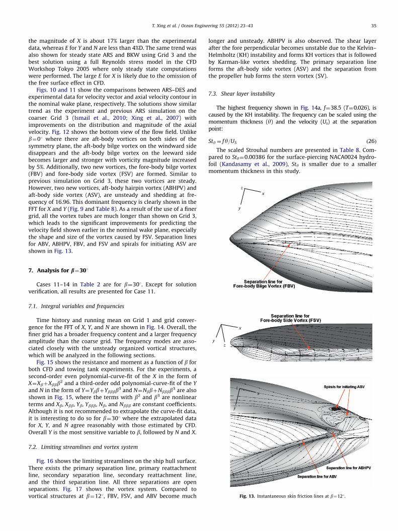
Figs. 10 and 11 show the comparisons between ARS–DES andexperimental data for velocity vector and axial velocity contour inthe nominal wake plane, respectively. The solutions show similartrend as the experiment and previous ARS simulation on thecoarser Grid 3 (Ismail et al., 2010; Xing et al., 2007) withimprovements on the distribution and magnitude of the axialvelocity. Fig. 12 shows the bottom view of the flow field. Unlikeb¼01 where there are aft-body vortices on both sides of thesymmetry plane, the aft-body bilge vortex on the windward sidedisappears and the aft-body bilge vortex on the leeward sidebecomes larger and stronger with vorticity magnitude increasedby 5%. Additionally, two new vortices, the fore-body bilge vortex(FBV) and fore-body side vortex (FSV) are formed. Similar toprevious simulation on Grid 3, these two vortices are steady.However, two new vortices, aft-body hairpin vortex (ABHPV) andaft-body side vortex (ASV), are unsteady and shedding at fre-quency of 16.96. This dominant frequency is clearly shown in theFFT for X and Y (Fig. 9 and Table 8). As a result of the use of a finergrid, all the vortex tubes are much longer than shown on Grid 3,which leads to the significant improvements for predicting thevelocity field shown earlier in the nominal wake plane, especiallythe shape and size of the vortex caused by FSV. Separation linesfor ABV, ABHPV, FBV, and FSV and spirals for initiating ASV areshown in Fig. 13.

x

yz

x

y

z

Fig. 13. Instantaneous skin friction lines at b¼121.

7. Analysis for b¼301

Cases 11–14 in Table 2 are for b¼301. Except for solutionverification, all results are presented for Case 11.

7.1. Integral variables and frequencies

Time history and running mean on Grid 1 and grid conver-gence for the FFT of X, Y, and N are shown in Fig. 14. Overall, thefiner grid has a broader frequency content and a larger frequencyamplitude than the coarse grid. The frequency modes are asso-ciated closely with the unsteady organized vortical structures,which will be analyzed in the following sections.

Fig. 15 shows the resistance and moment as a function of b forboth CFD and towing tank experiments. For the experiments, asecond-order even polynomial-curve-fit of the X in the form ofX¼XbþXbbb2 and a third-order odd polynomial-curve-fit of the Y

and N in the form of Y¼YbbþYbbbb3 and N¼NbbþNbbbb3 are alsoshown in Fig. 15, where the terms with b2 and b3 are nonlinearterms and Xb, Xbb, Yb, Ybbb, Nb, and Nbbb are constant coefficients.Although it is not recommended to extrapolate the curve-fit data,it is interesting to do so for b¼301 where the extrapolated datafor X, Y, and N agree reasonably with those estimated by CFD.Overall Y is the most sensitive variable to b, followed by N and X.

7.2. Limiting streamlines and vortex system

Fig. 16 shows the limiting streamlines on the ship hull surface.There exists the primary separation line, primary reattachmentline, secondary separation line, secondary reattachment line,and the third separation line. All three separations are openseparations. Fig. 17 shows the vortex system. Compared tovortical structures at b¼121, FBV, FSV, and ABV become much

longer and unsteady. ABHPV is also observed. The shear layerafter the fore perpendicular becomes unstable due to the Kelvin–Helmholtz (KH) instability and forms KH vortices that is followedby Karman-like vortex shedding. The primary separation lineforms the aft-body side vortex (ASV) and the separation fromthe propeller hub forms the stern vortex (SV).

7.3. Shear layer instability

The highest frequency shown in Fig. 14a, f¼38.5 (T¼0.026), iscaused by the KH instability. The frequency can be scaled using themomentum thickness (y) and the velocity (Us) at the separationpoint:

Sty ¼ fy=US ð26Þ

The scaled Strouhal numbers are presented in Table 8. Com-pared to Sty¼0.00386 for the surface-piercing NACA0024 hydro-foil (Kandasamy et al., 2009), Sty is smaller due to a smallermomentum thickness in this study.

Fig. 14. Time history and running mean on Grid 1 and FFT for Grids 1 to 4 at b¼301: (a) X, (b) Y and (c) N.


7.4. Karman-like shedding instability

The dominant frequency at f¼17.9 (T¼0.056) is caused by theKarman-Like vortex shedding instability that is due to interactionbetween opposite signed vortices (Sigurdson, 1995). The relation-ship between the shear layer instability and the Karman-like

shedding instability is that two vortices generated by the shear-layer instabilities near the ship bow merge together and forma new bigger vortex, which reattaches the ship hull and then shedfollowing the Karman-like frequency. The Karman-like vortexshedding frequency is lower than the KH frequency due to thelarger vortex size and smaller convection velocity. As suggested

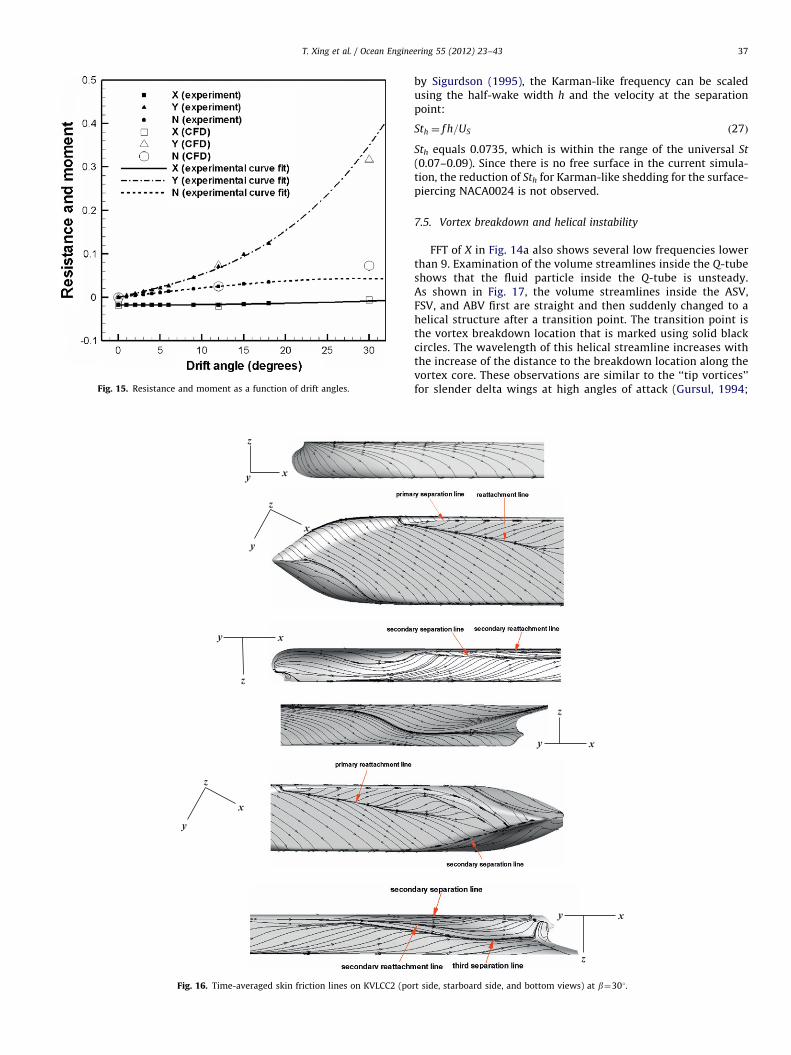
Fig. 15. Resistance and moment as a function of drift angles.

z

xy

yx

z

z

xy

y

x

z

Fig. 16. Time-averaged skin friction lines on KVLCC2 (po


by Sigurdson (1995), the Karman-like frequency can be scaledusing the half-wake width h and the velocity at the separationpoint:

Sth ¼ f h=US ð27Þ

Sth equals 0.0735, which is within the range of the universal St

(0.07–0.09). Since there is no free surface in the current simula-tion, the reduction of Sth for Karman-like shedding for the surface-piercing NACA0024 is not observed.

7.5. Vortex breakdown and helical instability

FFT of X in Fig. 14a also shows several low frequencies lowerthan 9. Examination of the volume streamlines inside the Q-tubeshows that the fluid particle inside the Q-tube is unsteady.As shown in Fig. 17, the volume streamlines inside the ASV,FSV, and ABV first are straight and then suddenly changed to ahelical structure after a transition point. The transition point isthe vortex breakdown location that is marked using solid blackcircles. The wavelength of this helical streamline increases withthe increase of the distance to the breakdown location along thevortex core. These observations are similar to the ‘‘tip vortices’’for slender delta wings at high angles of attack (Gursul, 1994;

z

xy

z

xy

rt side, starboard side, and bottom views) at b¼301.

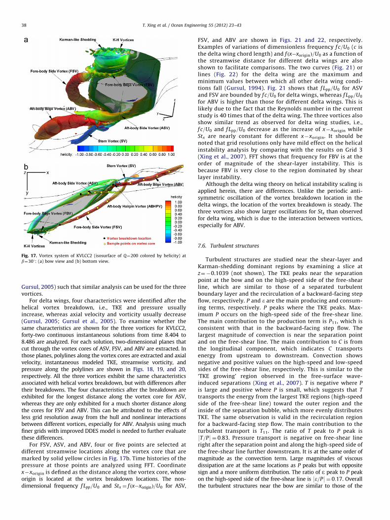
Fig. 17. Vortex system of KVLCC2 (isosurface of Q¼200 colored by helicity) at

b¼301: (a) bow view and (b) bottom view.


Gursul, 2005) such that similar analysis can be used for the threevortices.

For delta wings, four characteristics were identified after thehelical vortex breakdown, i.e., TKE and pressure usuallyincrease, whereas axial velocity and vorticity usually decrease(Gursul, 2005; Gursul et al., 2005). To examine whether thesame characteristics are shown for the three vortices for KVLCC2,forty-two continuous instantaneous solutions from time 8.404 to8.486 are analyzed. For each solution, two-dimensional planes thatcut through the vortex cores of ASV, FSV, and ABV are extracted. Inthose planes, polylines along the vortex cores are extracted and axialvelocity, instantaneous modeled TKE, streamwise vorticity, andpressure along the polylines are shown in Figs. 18, 19, and 20,respectively. All the three vortices exhibit the same characteristicsassociated with helical vortex breakdown, but with differences aftertheir breakdowns. The four characteristics after the breakdown areexhibited for the longest distance along the vortex core for ASV,whereas they are only exhibited for a much shorter distance alongthe cores for FSV and ABV. This can be attributed to the effects ofless grid resolution away from the hull and nonlinear interactionsbetween different vortices, especially for ABV. Analysis using muchfiner grids with improved DDES model is needed to further evaluatethese differences.

For FSV, ASV, and ABV, four or five points are selected atdifferent streamwise locations along the vortex core that aremarked by solid yellow circles in Fig. 17b. Time histories of thepressure at those points are analyzed using FFT. Coordinatex�xorigin is defined as the distance along the vortex core, whoseorigin is located at the vortex breakdown locations. The non-dimensional frequency f Lpp=U0 and Stx ¼ f ðx�xoriginÞ=U0 for ASV,

FSV, and ABV are shown in Figs. 21 and 22, respectively.Examples of variations of dimensionless frequency f c=U0 (c isthe delta wing chord length) and f ðx�xoriginÞ=U0 as a function ofthe streamwise distance for different delta wings are alsoshown to facilitate comparisons. The two curves (Fig. 21) orlines (Fig. 22) for the delta wing are the maximum andminimum values between which all other delta wing condi-tions fall (Gursul, 1994). Fig. 21 shows that f Lpp=U0 for ASVand FSV are bounded by f c=U0 for delta wings, whereas f Lpp=U0

for ABV is higher than those for different delta wings. This islikely due to the fact that the Reynolds number in the currentstudy is 40 times that of the delta wing. The three vortices alsoshow similar trend as observed for delta wing studies, i.e.,f c=U0 and f Lpp=U0 decrease as the increase of x�xorigin whileStx are nearly constant for different x�xorigin. It should benoted that grid resolutions only have mild effect on the helicalinstability analysis by comparing with the results on Grid 3(Xing et al., 2007). FFT shows that frequency for FBV is at theorder of magnitude of the shear-layer instability. This isbecause FBV is very close to the region dominated by shearlayer instability.

Although the delta wing theory on helical instability scaling isapplied herein, there are differences. Unlike the periodic anti-symmetric oscillation of the vortex breakdown location in thedelta wings, the location of the vortex breakdown is steady. Thethree vortices also show larger oscillations for Stx than observedfor delta wing, which is due to the interaction between vortices,especially for ABV.

7.6. Turbulent structures

Turbulent structures are studied near the shear-layer andKarman-shedding dominant regions by examining a slice atz¼�0.1039 (not shown). The TKE peaks near the separationpoint at the bow and on the high-speed side of the free-shearline, which are similar to those of a separated turbulentboundary layer and the recirculation of a backward-facing stepflow, respectively. P and e are the main producing and consum-ing terms, respectively. P peaks where the TKE peaks. Max-imum P occurs on the high-speed side of the free-shear line.The main contribution to the production term is P11, which isconsistent with that in the backward-facing step flow. Thelargest magnitude of convection is near the separation pointand on the free-shear line. The main contribution to C is fromthe longitudinal component, which indicates C transportsenergy from upstream to downstream. Convection showsnegative and positive values on the high-speed and low-speedsides of the free-shear line, respectively. This is similar to the‘TKE growing’ region observed in the free-surface wave-induced separations (Xing et al., 2007). T is negative where P

is large and positive where P is small, which suggests that T

transports the energy from the largest TKE regions (high-speedside of the free-shear line) toward the outer region and theinside of the separation bubble, which more evenly distributesTKE. The same observation is valid in the recirculation regionfor a backward-facing step flow. The main contribution to theturbulent transport is T11. The ratio of T peak to P peak is9T=P9¼ 0:83. Pressure transport is negative on free-shear lineright after the separation point and along the high-speed side ofthe free-shear line further downstream. It is at the same order ofmagnitude as the convection term. Large magnitudes of viscousdissipation are at the same locations as P peaks but with oppositesign and a more uniform distribution. The ratio of e peak to P peakon the high-speed side of the free-shear line is 9e=P9¼ 0:17. Overallthe turbulent structures near the bow are similar to those of the

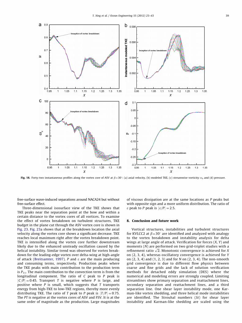
Fig. 18. Forty-two instantaneous profiles along the vortex core of ASV at b¼301: (a) axial velocity, (b) modeled TKE, (c) streamwise vorticity ox and (d) pressure.


free-surface wave-induced separations around NACA24 but withoutfree-surface effect.

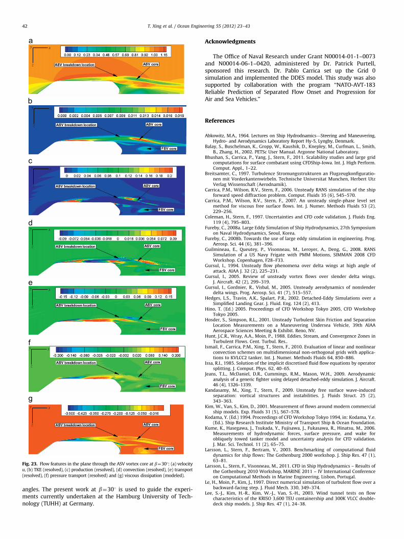
Three-dimensional isosurface view of the TKE shows thatTKE peaks near the separation point at the bow and within acertain distance to the vortex cores of all vortices. To examinethe effect of vortex breakdown on turbulent structures, TKEbudget in the plane cut through the ASV vortex core is shown inFig. 23. Fig. 23a shows that at the breakdown location the axialvelocity along the vortex core shows a significant decrease. TKEreaches local maximum right after the vortex breakdown point.TKE is intensified along the vortex core further downstreamlikely due to the enhanced unsteady oscillation caused by thehelical instability. Similar trend was observed for vortex break-down for the leading-edge vortex over delta-wing at high-angleof attack (Breitsamter, 1997). P and e are the main producingand consuming terms, respectively. Production peaks wherethe TKE peaks with main contribution to the production termis P11. The main contribution to the convection term is from thelongitudinal component. The ratio of C peak to P peak is9C=P9¼ 0:45. Transport T is negative where P is large, andpositive where P is small, which suggests that T transportsenergy from high-TKE to low-TKE regions, thereby more evenlydistributing TKE. The ratio of T peak to P peak is 9T=P9¼ 0:75.The PT is negative at the vortex cores of ASV and FSV. It is at thesame order of magnitude as the production. Large magnitudes

of viscous dissipation are at the same locations as P peaks butwith opposite sign and a more uniform distribution. The ratio ofe peak to P peak is 9e=P9¼ 2:5.

8. Conclusion and future work

Vortical structures, instabilities and turbulent structuresfor KVLCC2 at b¼301 are identified and analyzed with analogyto the vortex breakdown and instability analysis for deltawings at large angle of attack. Verification for forces (X, Y) andmoments (N) are performed on two grid-triplet studies with arefinement ratio

ffiffiffi2p

. Monotonic convergence is achieved for X

on (2, 3, 4), whereas oscillatory convergence is achieved for Y

on (2, 3, 4) and (1, 2, 3) and for N on (2, 3, 4). The non-smoothgrid convergence is due to different flow physics betweencoarse and fine grids and the lack of solution verificationmethods for detached eddy simulation (DES) where thenumerical and modeling errors are strongly coupled. Limitingstreamlines show primary separation and reattachment lines,secondary separation and reattachment lines, and a thirdseparation line. One shear layer instability mode, one Kar-man-like vortex shedding, and three helical mode instabilitiesare identified. The Strouhal numbers (St) for shear layerinstability and Karman-like shedding are scaled using the

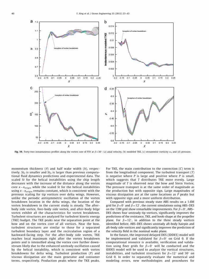
Fig. 19. Forty-two instantaneous profiles along the vortex core of FSV at b¼301: (a) axial velocity, (b) modeled TKE, (c) streamwise vorticity ox and (d) pressure.


momentum thickness (y) and half wake width (h), respec-tively. Sty is smaller and Sth is larger than previous computa-tional fluid dynamics predictions and experimental data. Thescaled St for the helical instabilities using the ship lengthdecreases with the increase of the distance along the vortexcore x�xorigin while the scaled St for the helical instabilitiesusing x�xorigin remains constant, which is consistent with theprevious scaling for tip vortices over delta wings. However,unlike the periodic antisymmetric oscillation of the vortexbreakdown location in the delta wings, the location of thevortex breakdown in the current study is steady. The after-body side vortex, fore-body side vortex, and after-body bilgevortex exhibit all the characteristics for vortex breakdown.Turbulent structures are analyzed for turbulent kinetic energy(TKE) budget. The TKE peaks near the separation point at thebow and on the vortex core of all vortices. Near the bow,turbulent structures are similar to those for a separatedturbulent boundary layer and the recirculation region of abackward-facing step. For the after-body side vortex, TKEreaches local maximum right after the vortex breakdownpoints and is intensified along the vortex core further down-stream likely due to the enhanced unsteady oscillation causedby the helical instability, which is consistent with vortexbreakdowns for delta wing. Turbulent production (P) andviscous dissipation are the main generator and consumerterms, respectively. Production peaks where the TKE peaks.

For TKE, the main contribution to the convection (C) term isfrom the longitudinal component. The turbulent transport (T)is negative where P is large and positive where P is small,which suggests that T distributes TKE more evenly. Largemagnitude of T is observed near the bow and Stern Vortex.The pressure transport is at the same order of magnitude asthe production but with opposite sign. Large magnitudes ofviscous dissipation are at the same locations as P peaks butwith opposite sign and a more uniform distribution.

Compared with previous steady state ARS results on a 1.6Mgrid for b¼01 and b¼121, the current simulations using ARS–DESon the 13M grid show remarkable improvements. For b¼01, ARS–DES shows four unsteady tip vortices, significantly improves thepredictions of the resistance, TKE, and hook-shape at the propellerplane. For b¼121, in addition to the three steady vorticesidentified before, ARS–DES shows unsteady aft-body hairpin andaft-body side vortices and significantly improves the prediction ofthe velocity field in the nominal wake plane.

In the future, the improved delayed DES (IDDES) model willbe implemented and validated for b¼01 on Grid 0. If thecomputational resource is available, verification and valida-tion using finer grids for b¼01 will be conducted and theIDDES model will be used to analyze the vortical structures,instabilities, and turbulent structures for b¼121 and 301 onGrid 0. In order to separately evaluate the numerical andmodeling errors, new methodologies and procedures for

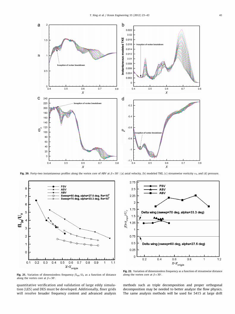
Fig. 21. Variation of dimensionless frequency f Lpp=U0 as a function of distance

along the vortex core at b¼301.

Fig. 22. Variation of dimensionless frequency as a function of streamwise distance

along the vortex core at b¼301.

Fig. 20. Forty-two instantaneous profiles along the vortex core of ABV at b¼301: (a) axial velocity, (b) modeled TKE, (c) streamwise vorticity ox and (d) pressure.


quantitative verification and validation of large eddy simula-tion (LES) and DES must be developed. Additionally, finer gridswill resolve broader frequency content and advanced analysis

methods such as triple decomposition and proper orthogonaldecomposition may be needed to better analyze the flow physics.The same analysis methods will be used for 5415 at large drift

z

y x

z

y x

z

y x

z

y x

z

y x

z

y x

z

y x

Fig. 23. Flow features in the plane through the ASV vortex core at b¼301: (a) velocity

u, (b) TKE (resolved), (c) production (resolved), (d) convection (resolved), (e) transport

(resolved), (f) pressure transport (resolved) and (g) viscous dissipation (modeled).


angles. The present work at b¼301 is used to guide the experi-ments currently undertaken at the Hamburg University of Tech-nology (TUHH) at Germany.

Acknowledgments

The Office of Naval Research under Grant N00014-01-1–0073and N00014-06-1–0420, administered by Dr. Patrick Purtell,sponsored this research. Dr. Pablo Carrica set up the Grid 0simulation and implemented the DDES model. This study was alsosupported by collaboration with the program ‘‘NATO-AVT-183Reliable Prediction of Separated Flow Onset and Progression forAir and Sea Vehicles.’’

References

Abkowitz, M.A., 1964. Lectures on Ship Hydrodnamics—Steering and Maneuvering,Hydro- and Aerodynamics Laboratory Report Hy-5, Lyngby, Denmark.

Balay, S., Buschelman, K., Gropp, W., Kaushik, D., Knepley, M., Curfman, L., Smith,B., Zhang, H., 2002. PETSc User Manual. Argonne National Laboratory.

Bhushan, S., Carrica, P., Yang, J., Stern, F., 2011. Scalability studies and large gridcomputations for surface combatant using CFDShip-Iowa. Int. J. High Perform.Comput. Appl., 1–22.

Breitsamter, C., 1997. Turbulence Stromungsstrukturen an Flugzeugkonfiguratio-nen mit Vorderkantenwirbeln. Technische Universitat Munchen, Herbert UtzVerlag Wissenschaft (Aerodnamik).

Carrica, P.M., Wilson, R.V., Stern, F., 2006. Unsteady RANS simulation of the shipforward speed diffraction problem. Comput. Fluids 35 (6), 545–570.

Carrica, P.M., Wilson, R.V., Stern, F., 2007. An unsteady single-phase level setmethod for viscous free surface flows. Int. J. Numer. Methods Fluids 53 (2),229–256.

Coleman, H., Stern, F., 1997. Uncertainties and CFD code validation. J. Fluids Eng.119 (4), 795–803.

Fureby, C., 2008a. Large Eddy Simulation of Ship Hydrodynamics, 27th Symposiumon Naval Hydrodynamics, Seoul, Korea.

Fureby, C., 2008b. Towards the use of large eddy simulation in engineering. Prog.Aerosp. Sci. 44 (6), 381–396.

Guilmineau, E., Queutey, P., Visonneau, M., Leroyer, A., Deng, G., 2008. RANSSimulation of a US Navy Frigate with PMM Motions, SIMMAN 2008 CFDWorkshop. Copenhagen, F28–F33.

Gursul, I., 1994. Unsteady flow phenomena over delta wings at high angle ofattack. AIAA J. 32 (2), 225–231.

Gursul, I., 2005. Review of unsteady vortex flows over slender delta wings.J. Aircraft. 42 (2), 299–319.

Gursul, I., Gordnier, R., Visbal, M., 2005. Unsteady aerodynamics of nonslenderdelta wings. Prog. Aerosp. Sci. 41 (7), 515–557.

Hedges, L.S., Travin, A.K., Spalart, P.R., 2002. Detached-Eddy Simulations over aSimplified Landing Gear. J. Fluid. Eng. 124 (2), 413.

Hino, T. (Ed.) 2005. Proceedings of CFD Workshop Tokyo 2005, CFD WorkshopTokyo 2005.

Hosder, S., Simpson, R.L., 2001. Unsteady Turbulent Skin Friction and SeparationLocation Measurements on a Maneuvering Undersea Vehicle, 39th AIAAAerospace Sciences Meeting & Exhibit. Reno, NV.

Hunt, J.C.R., Wray, A.A., Moin, P., 1988. Eddies, Stream, and Convergence Zones inTurbulent Flows. Cent. Turbul. Res..

Ismail, F., Carrica, P.M., Xing, T., Stern, F., 2010. Evaluation of linear and nonlinearconvection schemes on multidimensional non-orthogonal grids with applica-tions to KVLCC2 tanker. Int. J. Numer. Methods Fluids 64, 850–886.

Issa, R.I., 1985. Solution of the implicit discretised fluid flow equations by operatorsplitting. J. Comput. Phys. 62, 40–65.

Jeans, T.L., McDaniel, D.R., Cummings, R.M., Mason, W.H., 2009. Aerodynamicanalysis of a generic fighter using delayed detached-eddy simulation. J. Aircraft.46 (4), 1326–1339.

Kandasamy, M., Xing, T., Stern, F., 2009. Unsteady free surface wave-inducedseparation: vortical structures and instabilities. J. Fluids Struct. 25 (2),343–363.

Kim, W., Van, S., Kim, D., 2001. Measurement of flows around modern commercialship models. Exp. Fluids 31 (5), 567–578.

Kodama, Y. (Ed.) 1994. Proceedings of CFD Workshop Tokyo 1994, in: Kodama, Y.e.(Ed.). Ship Research Institute Ministry of Transport Ship & Ocean Foundation.

Kume, K., Hasegawa, J., Tsukada, Y., Fujisawa, J., Fukasawa, R., Hinatsu, M., 2006.Measurements of hydrodynamic forces, surface pressure, and wake forobliquely towed tanker model and uncertainty analysis for CFD validation.J. Mar. Sci. Technol. 11 (2), 65–75.

Larsson, L., Stern, F., Bertram, V., 2003. Benchmarking of computational fluiddynamics for ship flows: The Gothenburg 2000 workshop. J. Ship Res. 47 (1),63–81.

Larsson, L., Stern, F., Visonneau, M., 2011. CFD in Ship Hydrodynamics – Results ofthe Gothenburg 2010 Workshop, MARINE 2011 – IV International Conferenceon Computational Methods in Marine Engineering, Lisbon, Portugal.

Le, H., Moin, P., Kim, J., 1997. Direct numerical simulation of turbulent flow over abackward-facing step. J. Fluid Mech. 330, 349–374.

Lee, S.-J., Kim, H.-R., Kim, W.-J., Van, S.-H., 2003. Wind tunnel tests on flowcharacteristics of the KRISO 3,600 TEU containership and 300K VLCC double-deck ship models. J. Ship Res. 47 (1), 24–38.


Levy, Y., Degani, D., Seginer, A., 1990. Graphical visualization of vortical flows bymeans of helicity. AIAA J. 28 (8), 1347–1352.

Longo, J., Stern, F., 2002. Effects of drift angle on model ship flow. Exp. Fluids 32(5), 558–569.

Menke, M., Gursul, I., 1997. Unsteady nature of leading edge vortices. Phys. Fluids9 (10) 2960–2966.

Morton, S., Forsythe, J., Mitchell, A., Hajek, D., 2002. Detached-Eddy Simulationsand Reynolds-Averaged Navier–Stokes Simulations of Delta Wing VorticalFlowfields. J. Fluids Eng. 124 (4), 924.

Noack, R., 2005. SUGGAR: a General Capability for Moving Body Overset GridAssembly, 17th AIAA Computational Fluid Dynamics Conference.

Noack, R., 2009. Improvements to SUGGAR and DiRTlib for Overset Store Separa-tion Simulations, 47th AIAA Aerospace Sciences Meeting Including the NewHorizons Forum and Aerospace Exposition.

Pinto-Heredero, A., Xing, T., Stern, F., 2010. URANS and DES analysis for a Wigleyhull at extreme drift angles. J. Mar. Sci. Technol..

Sakamoto, N., 2009. URANS and DES Simulations of Static and Dynamics Maneu-vering for Surface Combatant, Department of Mechanical Engineering. TheUniversity of Iowa, Iowa City.

Sakamoto, N., Carrica, P.M., Stern, F., 2008. URANS Simulations of Static andDynamic Maneuvering for Surface Combatant, SIMMAN 2008, Copenhagen,pp. F49–F54.

Shur, M., Spalart, P.R., Strelets, M., Travin, A., 1999. Detached-eddy simulation ofan airfoil at high angle of attack. In: Rodi, W., Laurence, D. (Eds.), 4thInternational Symposium on Engineering Turbulence Modeling and Measure-ments, Corsica. Elsevier, Amsterdam, pp. 669–678.

Sigurdson, L.W., 1995. Structure and control of a turbulent reattaching flow.J. Fluid Mech. 298, 139–165.

Simonsen, C., Stern, F., 2005. Flow pattern around an appended tanker hull form insimple maneuvering conditions. Comput. Fluids 34 (2), 169–198.

Simonsen, C.D., Stern, F., 2003. Verification and validation of RANS maneuveringsimulation of Esso Osaka: effects of drift and rudder angle on forces andmoments. Comput. Fluids 32 (10), 1325–1356.

Stern, F., Agdrup, K., Kim, S.Y., Hochbaum, A.C., Rhee, K.P., Quadvlieg, F., Perdon, P.,Hino, T., Broglia, R., Gorski, J., 2011. Experience from SIMMAN 2008—the first

workshop on verification and validation of ship maneuvering simulationmethods. J. Ship Res. 55 (2), 135–147.

Stern, F., Wilson, R., Shao, J., 2006. Quantitative V&V of CFD simulations andcertification of CFD codes. Int. J. Numer. Methods Fluids 50 (11), 1335–1355.

Tahara, Y., Longo, J., Stern, F., 2002. Comparison of CFD and EFD for the Series 60CB¼0.6 in Steady Drift Motion. J. Mar. Sci. Technol. 7 (1), 17–30.

Tahara, Y., Stern, F., 1996. A large-domain approach for calculating ship boundarylayers and wakes and wave fields for nonzero froude number. J. Comput. Phys.127 (2), 398–411.

Toda, Y., Stern, F., Longo, J., 1992. Mean-flow measurements in the boundary layerand wake and wave field of a series 60 CB¼ 0.6 ship model-Part 1: Froudenumbers 0.16 and 0.316. J. Ship Res. 36 (4), 360–377.

Travin, A., Shur, M., Strelets, M., 2002. Physical and Numerical Upgrades in theDetached Eddy Simulation of Complex Turbulent Flows, in: Friedrich, R., Rodi,W. (Ed.), Advances in LES of Complex Flows, pp. 239–254.

Wallin, S., Johansson, A.V., 2000. An explicit algebraic Reynolds stress model forincompressible and compressible turbulent flows. J. Fluid Mech. 403, 89–132.

Wilson, R.V., Stern, F., Coleman, H.W., Paterson, E.G., 2001. Comprehensiveapproach to verification and validation of CFD simulations - Part 2: Applicationfor RANS simulation of a Cargo/Container ship. J. Fluids Eng. 123 (4), 803–810.

Xing, T., Kandasamy, M., Stern, F., 2007. Unsteady free-surface wave-inducedseparation: analysis of turbulent structures using detached eddy simulationand single-phase level set. J. Turbul. 8 (44), 1–35.

Xing, T., Shao, J., and Stern, F., 2007. BKW- RS-DES of Unsteady Vortical Flow forKVLCC2 at Large Drift Angles, the 9th International Conference on NumericalShip Hydrodynamics, Ann Arbor, Michigan.

Xing, T., Stern, F., 2010. Factors of safety for Richardson extrapolation. J. Fluids Eng.132 (6), 061403.

Xing, T., Stern, F., 2011. Closure to ‘‘Discussion of ‘Factors of Safety for RichardsonExtrapolation’’’ (2011, ASME J. Fluids Eng., 133, p. 115501). ASME Journal ofFluids Engineering 133 (11), 115502.

Yoon, H.Y., 2009. Force/Moment and Phase-Averaged Stereo PIV Flow Measure-ments for Surface Combatant in PMM Maneuvers, IIHR-Hydroscience &Engineering. The University of Iowa, Iowa City, Iowa, USA.

Documents

Vortical and turbulent structures for KVLCC2 at drift ... · Vortical and turbulent structures for KVLCC2 at drift angle 0, 12, and 30 degrees Tao Xinga,n, Shanti Bhushanb, Frederick