29th

Symposium on Naval Hydrodynamics

Gothenburg, Sweden, 26-31 August 2012

Vortex Cavitation Inception Delay by

Local Polymer Injection

G. L. Chahine, C.-T. Hsiao, X. Wu, Q, Zhang, and J. Ma

(DYNAFLOW, INC., USA)

ABSTRACT

The effects of polymer injection on vortex cavitation

inception were studied both experimentally and

numerically. Experimentally, a vortex chamber

equipped with a polymer injection port on the axis

enabled study of the effect of local polymer injection

on cavitation inception. The injection flow rates and

polymer concentrations required to delay cavitation in

the vortex core were investigated for different vortex

strengths. Numerically, a viscoelastic FENE-P model

was coupled with a transport equation of the polymer

concentration to track the distribution of the injected

polymer solution in the flow field versus time. Both

the experimental and numerical studies were able to

show that injection of dilute polymer solutions can

delay cavitation inception using a much lower solution

injection flow rates than necessary with massive

injection of water or of a high viscosity liquid. Flow

visualizations and numerical simulations also strongly

indicated that a phenomenon responsible for the strong

modification of the flow character is the much earlier

occurrence of vortex breakdown in the case of the

polymer solution, probably due to the elastic

properties of the polymers. These induce fast

reduction of the rotational velocities, increase of the

pressures, and delay of cavitation inception.

INTRODUCTION

Tip vortex cavitation is often observed as the first

form of cavitation on a propeller and is therefore

targeted first for cavitation inception delay. Laboratory

tests have shown that if the bulk liquid is made of a

dilute solution of polymers cavitation inception is

delayed through both reduction of the vortex

circulation and thickening and slowing down the

rotation of the vortex viscous core (Fruman and

Aflalo, 1989).

Local injection of polymer solutions in the tip

region of a 3D foil was also shown to be effective in

delaying the tip vortex cavitation inception without

affecting the lift. This was demonstrated on elliptic

foils by Fruman and Aflalo (1989), Fruman et al.

(1995), and Latorre et al. (2004). To our knowledge

only the study reported by Chahine et al. (1993) has

demonstrated polymer injection beneficial effects on

cavitation inception on an actual propeller. However,

these studies could not completely elucidate the

mechanisms that resulted in the observed effects of tip

vortex cavitation inhibition. Due to the complexity of

a propeller flow, experimental measurements of the

velocity in the core region of the rotating vortical

structures are very challenging due to both the fluid

particles rotational motion and to the wandering of the

vortex core. Even for a tip vortex flow generated by a

fixed finite-span foil, the location of polymer injection

influences significantly the results.

To study the effect of polymer solution on a

vortex flow in a controlled laboratory environment,

Barbier and Chahine (2009) conducted experiments in

a specially designed swirl chamber. They showed that

with polymer solutions the inception of cavitation at

the center of the vortex required a higher flow rate

when compared to the same tests in water. Hsiao et al.

(2009) modified the design of the swirl chamber to

enable local injection of polymer solutions directly

into the vortex center such that the suppression of

vortex cavitation due to polymer injection matches

better with real applications. The study presented here

further improves the injection mechanism by using a

pneumatic actuator to better control the injection

timing and flow rate. This design coupled with high

speed photography observations, allowed us to better

identify the polymer concentrations and injection rates

required to suppress cavitation for different vortex

strengths, and to characterize the modifications to the

basic character of the flow field by the injection.

In parallel to the experimental studies, we also

present a numerical study to further help explain the

flow structure modification by the polymers. Zhang et

al. (2009) implemented a FENE-P model, Finite-

Extensibility-Nonlinear-Elasticity model with Peterlin

closure (Bird et al. 1987), in a Navier-Stokes solver to

study bulk polymer solutions viscoelastic effects on

the propeller tip vortex flow and on bubble dynamics.

To enable simulation of local polymer solutions

injection, Hsiao et al. (2009) solved a transport

equation of the polymer concentration to compute the

time and space variations of the polymer

concentrations in the flow field. This model is applied

here to the flow field of the swirl chamber equipped

with an axial injector. The vortex flow structure

changes due to the injection and the resulting polymer

stresses are investigated.

In this paper results from both experimental and

numerical studies are presented. These studies aim at

uncovering the underlying physics, which cause vortex

cavitation inception delay by local polymer injection..

EXPERIMENTAL STUDY

Experimental Setup

Experiments were conducted using a relatively large

vortex chamber (diameter 6 in. and length 12.9 in.).

Figure 1 shows a sketch of the vortex chamber

assembly with dimensions. Figure 2 shows a picture of

the vortex chamber.

The vortex chamber was made of acrylic for

better optical transparence; it had two concentric

cylindrical chambers with each end closed by an

acrylic plate. The two end plates had a circular orifice

opening each, all aligned with the chamber axis. A

larger orifice at one end served as flow outlet, while a

small orifice at the other end was used for polymer

injection. Table 1 shows the key dimensions of the

chamber.

Chamber length 12.9 in

Inner cylinder OD 6.0 in

Inner cylinder ID 5.5 in

Outer cylinder OD 8.0 in

Outer cylinder ID 7.5 in

Slot length 12.9 in

Slot height 0.078 in

Total number of slots 4

Angular positions of the slots

45o, 135

o,

225o, 315

o

Outlet orifice diameter 0.6 in

Injection orifice diameter 0.078 in

Tank liquid level 12 in

Outlet-tank wall distance 24 in

Table 1: List of key dimensions of the vortex chamber

used in the tests.

During operation, the fluid entered the space

between the two cylinders, and then was accelerated

tangentially into the inner chamber through four end-

to-end small area tangential slots, which generated a

swirling flow inside the inner cylinder. With increasing

flow rate, cavitation first occurred in a very thin

axially located rotating bubble, and then grew into a

cavitating vortex core, which fully covered the

centerline of the chamber from end to end. This

configuration made the vortex swirl intense and led to

early cavitation with a very stable core even at low

flow rates, suitable for experimental study.

The vortex chamber was submerged in a

14 x 14 x 40 in3 reservoir tank filled with liquid and

formed a closed loop with the help of a re-circulating

pump. More detailed description can be found in

(Hsiao et al. 2009).

Figure 1: Dimensions of the vortex chamber assembly

used for vortex cavitation inception studies.

Figure 2: Picture of the empty vortex chamber.

Figure 3: Sketch of the polymer injection control

scheme.

Polymer solutions were introduced into the

vortex core through the injection orifice. In order to

have good control on timing and volume injection, a

pneumatic actuator was used to control with a plug the

opening and closing of the injection orifice.

Figure 3 shows a sketch of the control

mechanism. When injection started, the polymer

solution was pushed into the vortex core under a

constant pressure provided by a relatively large

volume of compressed air. Figure 4 and Figure 5 show

a sketch and a picture of the experimental setup.

Figure 4: Sketch of the polymer injection scheme.

Figure 5: Picture of the experimental set up with

polymer injection.

An IDT High speed camera was used for flow

visualizations; it was capable of a framing rate from

2,000 fps (1,280 x 1,024 pixels) to 130,000 fps (1,280

x 16 pixels) and was synchronized with the polymer

injection controller.

For flow field velocity measurements, an Oxford

laser 35-30 PIV system was used to perform Particle

Image Velocimetry (PIV) measurements. The dual

head YAG laser (35 mJ/pulse at 532 nm wavelength,

repetition rate up to 30 Hz) was paired with a PCO

Pixelfly-QE CCD to capture the PIV images. The

camera had a resolution of 1,392 x 1,024 pixels (12-bit

digital output). The PIV velocity measurement

uncertainty was about 5%. Figure 6 shows a picture of

the experimental setup for flow field measurements

with the PIV system. An adaptive cross-correlation

analysis scheme, similar to the scheme used by Hsiao

et al. (2009), was utilized in the analysis.

Figure 6: Picture of the PIV camera mounted on a 3D

programmable motorized slide.

Cavitation Suppression

Using the experimental setup described above flow

visualizations were conducted to observe the

phenomena under different flow conditions. In

degassed water a gaseous core initialized as an

elongated bubble on the axis at a flow rate of about

12 gpm. The bubble wandered along and around the

chamber axis with intermittent appearance of other

bubbles on this axis. As the flow rate increased above

about 15 gpm, a cavitation vaporous core fills the

vortex chamber axis from end to end and forms a

tubular core. The uncertainty on the water flow

rate measurement was about 1%.

Cavitation suppression attempts are illustrated in

Figure 7 to Figure 9 respectively for local mass

injections of a Polyox solution, a water/glycerin

mixture, and water. All three cases are for a vortex

chamber water flow rate of 20 gpm, i.e. beyond

cavitation inception. Dye was mixed with the injected

solutions to enhance the visualization and for all three

cases the injection rate was 600 ml/min. The

uncertainty on the injection flow rate was about

1%.Figure 7 shows the case on a 1,000 ppm polymer

solution injection at an injection rate of 600 ml/min.

As can be seen in the sequence of three photos from a

recorded movie, 3 seconds after the start of the

injection (mid picture) the core size begins to shrink,

and disappears completely after 6 seconds (bottom

picture). This picture shows that the injected Polyox

Compressed air

High speed camera

Reservoir tank

DYNASWIRL® chamber

Polymer tank

Injection controller

highlighted by the colored dark dye (grey in the

picture) remains in the now liquid-only viscous core of

the line vortex.

In order to investigate whether the observed effect

in Figure 7 is due to the higher viscosity of the

injected polymer solution, Figure 8 shows a similar

time sequence at 0, 3, and 6 seconds after injection of

a solution of water and corn syrup with the same

viscosity as that of the polymer solution. It can be seen

that in this case, the dyed corn syrup solution wrapped

around the cavitating core, thinned the core diameter,

but did not succeed in suppressing cavitation as clearly

seen after 6 seconds.

Finally, Figure 9 shows the effect of the injection

of only water on the vortex behavior. As compared to

the Figure 8 results, injection of water has an even

lesser effect than the corn syrup solution on the line

vortex cavitation. The injected dyed water can be seen

diffusing around the vaporous core and affecting little

cavitation.

Figure 7: Time sequence pictures of the effect of

polymer injection on the cavitation core (1,000 ppm

polyox, 600 ml/min injection rate, 20 gpm liquid flow

rate). From top to bottom: 0, 3, and 6 s. after start of

injection. Injection included a dye which can be seen

in the last picture after cavitation suppression.

Figure 8: Time sequence pictures of the effect of corn

syrup injection on the cavitation core (solution has

same viscosity as the 1000 ppm Polyox solution in

Figure 7, 600 ml/min injection rate, 20 gpm liquid

flow rate). From top to bottom: 0, 3, and 6 s. after

start of injection. Injection included a dye which can

be seen always present around cavitation core.

Figure 9: Time sequence pictures of the effect of

water injection on the cavitation core (600 ml/min

injection rate, 20 gpm liquid flow rate). From top to

bottom: 0, 3, and 6 s. after start of injection. Injection

included a dye which can be seen always present

around cavitation core.

Previous studies, for instance by Platzer and

Souders (1979), and more recent work by Chang et al

(2011) have shown that massive injection of water can

also delay and suppress cavitation inception in tip

vortex flows. To examine this effect, we conducted

tests will higher injection rates of water.

Figure 10 illustrates the line vortex cavitation for

a vortex chamber flow rate of 18 gpm at the highest

water injection flow rate that we could achieve in the

facility described above. This corresponded to an

injection rate of 2,200 ml/min. Even at this high

injection rate the core did not disappear completely.

The cavitation core was affected by the water

injection, it strongly wandered around, broke from a

continuous core into a disrupted vaporous core, but the

cavitation did not disappear.

Figure 10: Time sequence pictures of the effect of

water injection on cavitation core (2,200 ml/min

injection rate, 18 gpm liquid flow rate). From top to

bottom: 0, 3, and 6 s. after start of injection. Injection

included a dye which can be seen around always

present cavitation core.

The above observations illustrate that polymer

effects on the vortex cavitation are mainly due not to

viscous or mass injection effects, but mainly to

viscoelastic effects that produce stresses inexistent

with viscous liquid only.

Another means of representing the effect of

polymer injection on the line vortex cavitation core is

to observe the length of the vaporous core under

various operating conditions. For a given vortex

strength (given liquid flow rate into the swirl chamber)

as the polymer injection rate approaches the value

required to suppress cavitation, the vaporous core

starts to partially disappear from one end of the

cylindrical chamber. The length of the core oscillates

around a mean value, which can be directly related to

the combination polymer injection rate and flow rate.

Figure 11 illustrates and characterizes this

behavior. It shows the reduction of the core length

from a given developed cavitation condition. For zero

injection the length reduction is zero, and as the rate

increases the reduction increases too, attaining 100%

when the required injection rate for cavitation

suppression is achieved. The figure is shown for a

polymer solution of 1,000 ppm and for various vortex

strengths. The figure also shows that, for a given

polymer injection rate, the lower the liquid flow rate

into (equivalent to lower rotational speed) the

DYNASWIRL® chamber, the higher the percentage of

the core length reduction.

Figure 11: Vortex core length reduction with the rate

of polymer injection into the vortex core for different

water flow rates. 1,000 ppm Polyox solution.

Figure 12 shows, for different swirl chamber

liquid flow rates, the amount of polymer solution to be

injected by unit time (injection rate) to completely

suppress the cavitation core. Four concentrations of

Polyox polymer solutions: 500 ppm, 1,000 ppm, 4,000

ppm, and 6,000 ppm are shown. As expected, for a

given polymer solution concentration the required

injection rate increase with the vortex strength (liquid

flow rate). As the concentration increases less polymer

solution is required. However, as the spacing between

the curves indicates, the rate appears to tend towards

an asymptote as the concentration exceeds 1,000 ppm.

While, there is a significant required polymer injection

rate difference between 500 ppm to 1000 ppm, there is

very little change between 1,000 and 4,000 and the

extra polymers injected above 1,000 ppm are wasted.

This saturation effect is common also in other

applications where viscoelasticity is important.

Figure 12: Required polymer injection rates to

completely suppress the cavitation at different polymer

solution concentrations and different vortex intensities

(liquid flow rate).

Figure 13: Required injected polymer mass to

completely suppress the cavitation at different polymer

solution concentrations and different vortex intensities

(liquid flow rate).

Figure 13 recasts the same data of Figure 12 in

terms of the injected mass rate of the polymers, i.e.

combines injection rate and concentration. The figure

shows that the lower concentrations considered (500

ppm and 1,000 ppm), are far more effective in

suppressing the cavitation than the higher

concentrations (4,000 ppm and 6,000 ppm), since the

higher concentrations consume much higher total

polymer mass to achieve the same effect.

Figure 14: Time sequence of dye diffusion from

injection of water at 0.01 sec (top), 2 sec (middle), and

4 sec (bottom) from the start of injection. The liquid

flow rate is 6 gpm and injection rate is 600 ml/min.

Figure 15: Time sequence of dye diffusion from

injection of a solution of 1,000 ppm of Polyox at 0.01

sec (top), 2 sec (middle), and 4 sec (bottom) from the

start of injection. The liquid flow rate is 6 gpm and

injection rate is 600 ml/min.

Diffusion of Injected Solution To understand better

how the injected solutions diffuse in the vortex flow,

dye was mixed with water, corn syrup, and the

polymer solutions as a flow visualization tracer. High

speed photography synchronized with injection

initialization was used to visualize the diffusion of the

dye after injection. Time sequence of dye diffusion

from injection of water and polymer are shown in

Error! Reference source not found. and Error!

Reference source not found.. The injection rate was

600 ml/min and the flow rate into the swirl chamber

was 6 gpm. The concentration of the polymer solution

was 1,000 ppm.

Each figure shows a snapshot at 0.01 sec. (top), 2

sec. (middle), and 4 sec. (bottom) from the start of

injection. As shown in the pictures, the diffusion of the

injected solution was much more concentrated for

water than from the polymer. The injected polymer

diffused more rapidly with much scattered flow

structure observed.

Much interesting, for the polymer solution and to

a lesser extent for water, three dimensional secondary

vortical structures including vortex rings and hairpin

vortices can be seen ejected from the vortex core (see

Figure 16). These will be very difficult to model

numerically.

Figure 16: Three dimensional secondary vortical

structures including vortex rings and hairpin vortices

ejected from the vortex core. Blow up at the edge of

the core, where dye is seen in Figure 15

Flow Field Measurements

The time-averaged velocity field was measured using

Particle Image Velocimetry (PIV) at different locations

in the swirl chamber. Figure 17 shows the tangential

velocity profiles in four planes along the chamber at

axial locations downstream of the injection orifice: X

= 8 cm, X = 16.5 cm (mid-plane of the vortex

chamber), X = 25.2 cm, and X = 30 cm. In each

measurement position, 600 double exposure image

pairs were obtained to get the average velocity

profiles. Even though the tangential injection slots

span the whole swirl chamber length and have a

constant opening size, the maximum tangential

velocity is seen in Figure 17 to increase in the

downstream direction (i.e. as the vortex flow

approaches the nozzle exit). As for the tip vortex flow

on a blade or foil, vorticity generated in the tangential

injection slots accumulate in the vortex core as the

distance increases from the start of the tangential

injection.

Figure 17: Variation of the tangential velocity in the

swirl chamber at different X locations measured

downstream from the end plate where polymer

injection is introduced. X=16.5 cm is the mid-plane of

the vortex chamber. Flow rate = 6 gpm.

Figure 18. Effect of the liquid flow rate on the

averaged tangential velocity profiles. X = 8 cm.

The influence of the tangential flow rate on the

velocity profiles can be seen in Figure 18 for both the

time-averaged tangential and radial velocities. The

profiles at the location X = 8 cm are shown. As

illustrated in the figure both the peak tangential

velocity and the core size (radial location of the peak)

increase with the tangential flow rate.

NUMERICAL STUDY

Governing Equations

The flow of a dilute, homogeneous and incompressible

polymer solution is described by the continuity and the

momentum conservation equations:

0u , (1)

2 1

Re Re

Dp

Dt

uu T , (2)

where u represents the fluid velocity, p the pressure, t

the time, and T the viscoelastic extra-stress tensor.

Equations (1) and (2) are in non-dimensional form

with a characteristic velocity, U, and characteristic

length, l. The Reynolds number, Re, is based on U, l

and the total viscosity, = s + p, where s is the

solvent (water) viscosity and p, is the extra shear

viscosity due to the polymer,

es p

UlR . (3)

The parameter is the ratio of solvent viscosity to the

total and is defined as:

/ .s (4)

The polymer stress T is normalized by /pU l .

The polymer stress tensor T is related to the

strain flow field through the constitutive equation of

the Finitely Extensible Nonlinear Elastic - Peterlin

(FENE-P) dumbbell model (Bird et al. 1987):

1

e

f aD

T C I , (5)

where C is the conformation tensor, defined as the

ensemble averaged dyad of the end-to-end distance of

the polymer chains. De is the Deborah (or

Weissenberg) number, which is the non-dimensional

relaxation time of the polymer

/eD l U, (6)

and f is the Peterlin function

2

2kk

LfL c

, (7)

where L is the extensibility parameter and kkc is the

trace of tensor C.

The conformation tensor C is governed by:

1T

c

Df a

Dt D

Cu C C u C I , (8)

in which the superscript T denotes the transpose. Since

the conformation tensor C is symmetric, only 6

components are computed.

The parameter a depends on L as follows,

2

1

31

a

L

. (9)

when L , FENE-P model recovers the Oldroyd-

B model (see Bird et al. 1987). In this study, L is set

to be 60, as used by Li et al. (2006).

The viscosity and the polymer stress will depend

on the local polymer solution concentration, especially

if the considered problem involves local polymer

injection. In this case, a transport equation of the

polymer concentration, c , needs to be solved:

2

e

1

Rc

cc c

t Su , (10)

where Sc is the Schmidt number defined by

scS D

, (11)

in which D is the diffusion coefficient of the polymer

molecules.

Numerical Method

To solve Equations (1) and (2), a three-dimensional

incompressible Navier-Stokes solver is exercised.

3DYNAFS-VIS©

includes in addition to viscoelastic

flow modeling, a moving overset grid scheme for

bubble dynamics problems, an Eulerian/Lagrangian

two-way coupling scheme for simulation of

bubble/liquid two phase flows, and a Level-Set

scheme for simulation of large-deformation free

surface flows.

3DYNAFS-VIS© is based on the artificial-

compressibility method (Chorin 1967), in which an

artificial time derivative of the pressure is added to the

continuity equation as:

10

c

p

tu , (12)

where c is the artificial compressibility factor. As a

consequence, the hyperbolic system of equations (1)

and (2) is formed and is solved using a time marching

scheme in the pseudo-time to reach a steady-state

solution. To obtain a time-dependent solution, a

Newton iterative procedure is performed at each

physical time step in order to satisfy the continuity

equation.

The numerical scheme in 3DYNAFS-VIS© uses a

finite volume formulation and is based on the code

UNCLE developed by Mississippi State University

(Arabshahi et al. 1995). A first-order Euler implicit

difference formula is applied to the time derivatives.

The spatial differencing of the convective terms uses

the flux-difference splitting scheme based on Roe’s

method (Roe 1981) and a van Leer’s MUSCL method

(van Leer 1979) for obtaining the first- or third-order

fluxes. A second-order central differencing is used for

the viscous terms, which are simplified using a thin-

layer approximation. The flux Jacobians required in an

implicit scheme are obtained numerically. The

resulting system of algebraic equations is solved using

a discretized Newton Relaxation method in which

symmetric block Gauss-Seidel sub-iterations are

performed before the solution is updated at each

Newton iteration.

In order to extend the Navier-Stokes solver to

non-Newtonian fluids, a time integration scheme of

Equation (8) to obtain the conformation tensor C and

the polymer stress tensor T, was implemented and

coupled to the original NS solver. The solution of the

constitutive and momentum equations and polymer

stress tensor T uses a staggered procedure, i.e. the

polymer contribution in Equation (2) is calculated at

each step once the velocity is known, then equation (2)

can be solved as normally done for the Navier-Stokes

equation, but with a body force term from the

divergence of the polymer stress.

At time step n, the velocity un, the pressure p

n,

and the polymer stress Tn

are known. Using nu Equation (8) can be integrated to provide the

conformation tensor for the next time step. A first

order differentiation in the time stepping, with time

step t is used:

1

1.

n nn

nT

t

f aDe

C Cu C

u C C u C I

(13)

A first order upwind scheme is used for the spatial

discretization of the convection term of Equation (13),

and a second order center difference scheme is used

for the velocity gradient. After obtaining Cn+1

the

polymer stress Tn+1

is calculated from Equation (5)

and the divergence of T is obtained. This provides the

polymer stress term in Equation (2):

11

Ren

polymerb T , (14)

and the momentum equation at step n+1 becomes:

11 2 1

Re

nn n

polymerD

pDt

uu b ,(15)

which has the same form as the Newtonian Navier-

Stokes equation.

Equation (15) is solved together with the

continuity equation to obtain the velocity un+1

and the

pressure. pn+1

. At this point, all the quantities for step

n+1 are known and a new loop starts with the

calculation of Cn+2

.

In order to model local polymer injection, we

need to solve Equation (10) in addition to the time

integration of Equation (8). Similar to solving

Equation (13), the concentration equation is integrated

at each time step once the velocity is known from the

Navier-Stokes equations:

1

2

e

1

R

nn n

c

c cc c

t Su . (16)

The convection term and the diffusion term are

discretized using respectively a first order upwind and

a second order central difference scheme. In the

simulations of local polymer injection, both the

Reynolds number, , and the Deborah number De

depend locally on the concentration, c , as detailed

below.

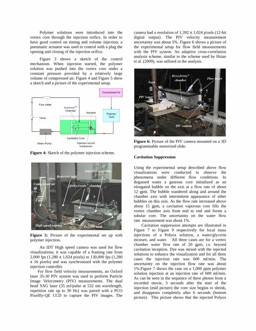
0.9

1.1

1.3

1.5

1.7

1.9

2.1

2.3

0 200 400 600 800 1000 1200

Polyox Concentration (ppm)

Vis

co

sit

y (

cp

)

Figure 19: Shear viscosity of Polyox WSR301

solution at different concentrations measured with the

dropping ball method.

Polymer Solution Properties

To simulate the flow, the viscosity and relaxation time

of the polymer solution are needed for different

polymer concentrations. Since Polyox WSR301 is

used in our experimental studies and is of interest in

tip vortex cavitation suppression, we measured the

total shear viscosity of Polyox solutions at different

concentrations using the falling-ball method, i.e. the

viscosity of liquid is deduced from the measurement

of the terminal velocity of a ball falling in the liquid

and using a Stokes flow assumption. Rigorously

speaking, the falling ball method is only applicable to

a Newtonian fluid. However, as suggested by Chhabra

(1993), in the case of shear-thinning viscoelastic

fluids, the drag on a sphere is largely determined by

the shear dependent viscosity and the viscoelasticity

exerts little influence at least for small values of

Deborah number. Therefore, we assume that the drag

force which balances with the ball weight and

buoyancy force is only caused by the total viscosity of

the polymer solutions without any elasticity effect.

Figure 19 shows the measured total viscosity at

different polymer concentrations.

The relaxation time of Polyox WSR301 has been

reported by Lindner et al. (2003) for concentration up

to 1,000 ppm. They found that in the dilute regime

(less than 500 ppm) the relaxation time can be treated

as constant ( ~0.0029 s). Another constant value

( ~0.0039 s) was found for concentrations between

500 ppm and 1,000 ppm.

injection

Figure 20: 3D view of the computational domain of

the vortex chamber flow.

Flow Field Computation

Throat

Swirl Chamber

Outside

Domain

By using the above polymer stress model and

numerical method, numerical simulations were

conducted to simulate the vortex flow field in the swirl

chamber described earlier in this paper. The

geometrical parameters summarized previously in

Table 1 were employed. The selected computational

domain is shown in Figure 20 and is composed of

three sections: the swirl chamber, the nozzle orifice,

and the outside domain. These are discretized with

91×81×121, 41×16×121 and 41×51×121 grid points

respectively. Near the swirl chamber walls and the

axis, much finer grids were used to capture the large

velocity gradients. All the results shown below were

obtained by unsteady simulations with the non-

dimensional divergence of velocity converging to

1x10-4

at each real time step.

The case with a 6 gpm flow rate tested in the

experiment without injection was simulated. The

Reynolds number based on water viscosity, orifice

outlet diameter, and average velocity at the outlet was 43.17 10 .

A snapshot of the tangential velocity along the

chamber longitudinal direction is shown in Figure 21.

Error! Reference source not found. shows a

comparison of tangential velocity profiles at the

middle of the swirl chamber between the PIV

measurements and the numerical solution. The time-

averaged solution was obtained from the unsteady

computation after removing the transient period for the

numerical results. The time-averaged solution was

deduced from the unsteady computation by excluding

the transient period for the numerical results. The full

3D simulations in the absence of turbulence model

were found to over-predict the tangential velocity

while the solution obtained by Large Eddy Simulation

(LES) captured well the velocity profile.

Figure 21: A snapshot of the water rotational

(tangential) velocity contours inside the vortex

chamber, indicating low velocities away from the

chamber axis (lowest horizontal line), and maximum

tangential velocity at the edge of the viscous core,

which extends inside the orifice of the left.

Simulation of Local Liquid Injection

We study here numerically, as in the experiments,

the effect of liquid injection into the vortex line core

on the vortex flow. Three liquid solutions are

considered: a) a 400ppm Polyox solution b) a solution

of water/corn syrup which has the same viscosity as

the Polyox solution but no Non-Newtonian effects,

and c) water. The liquids are injected into the swirl

chamber axis through a circular area as shown in

Figure 23.

For all three cases, simulations were conducted

for an injection flow rate of 1.3 ml/s and were started

from the same fully developed flow field obtained by a

water-only run in the absence of injection. The

simulations were mostly meant to study the effect of

the non-Newtonian polymer on the flow field, and to

examine differences relative to the injection of water

and a solution of water / corn syrup.

In the results presented below, axially symmetric

solutions are considered and three-dimensional effects

are neglected to speed up the numerical simulations

and concentrate the analysis on the polymer effects on

the vortex flow average solution, since as seen from

the visualizations, to fully resolve the flow field in the

swirl chamber an extremely fine grid is required in the

vortex core region and near the injection port.

Figure 22: Comparison of the tangential velocity

profiles between the PIV measured data and the

3DYNAFS-VIS©

solutions using either LES or no

turbulence model.

Figure 23: Snapshot of the contours of the polymer

concentration (normalized by 400ppm) in the vortex

chamber. The black circles indicate the monitored

locations.

For modeling polymer injection, the relaxation

time was set to 0.0029 sec. and the viscosity-

concentration relation shown in Figure 19 was used to

account for concentration effects, i.e. the Reynolds

number and were computed locally according to the

local polymer concentration. The 400 ppm Polyox

solution is injected from the inlet of the chamber, and

the polymer molecules are dispersed by the flow, i.e.,

spread axially and radially. After some time, as shown

in Figure 23, the vortex core fills up with polymer

solution of a lower concentration, while the liquid

outside of the core remain free of polymers.

Figure 24 compares, between the three injected

liquids, the most important quantity related to

cavitation, i.e. the evolution of the vaporous core

location (represented in this single-phase simulation,

by the iso-surface where the pressure is equal the

vapor pressure). The three time snapshots show that

with the polymer injection the core is remarkably

disrupted and ultimately disappears, while in the other

two cases, i.e., corn syrup and water, the original core

remains practically at the same location as before

injection. This result is in good agreement with the

experimental observations, previously presented.

Figure 24: Iso-surface of cp=-0.6 for the cases of

injection of polymer (top), corn syrup (middle), and

water (bottom).

The pressure contours in the vortex core region

displayed in Figure 25 illustrate well that the

disruption/suppression of the vaporous core in the

polymer injection case is due to the significant

pressure rise caused by the non-Newtonian effects,

which are not observed in the other two cases.

In order to further quantify the pressure rise effect

with the polymer injection, we examine the pressure

variations with time on the axis at the inlet (injection

location), center, and exit of the chamber axis for all

three injection cases. These fluctuations are compared

in Figure 26. While all behave is initially in a similar

fashion, the polymers modify significantly the

pressures at all three locations monitored after about

0.8s. This is probably the time required for the

polymers to reach the axial region of the vortex where,

as we will see below, the polymers are the most

effective and where vortex breakdown. The pressure

increases sometimes exceed the reference pressure

(i.e., pressure coefficient> 0). The pressures for the

other two injection cases have minor local oscillations

but no major average value modifications can be

observed.

Figure 25: Pressure contours of the pressure field near

the vortex line center for polymer (top), corn syrup

(middle), and water (bottom). The injection point is at

the right-lower corner of the domain. Scale is stretched

in the radial direction to highlight the region of

interest.

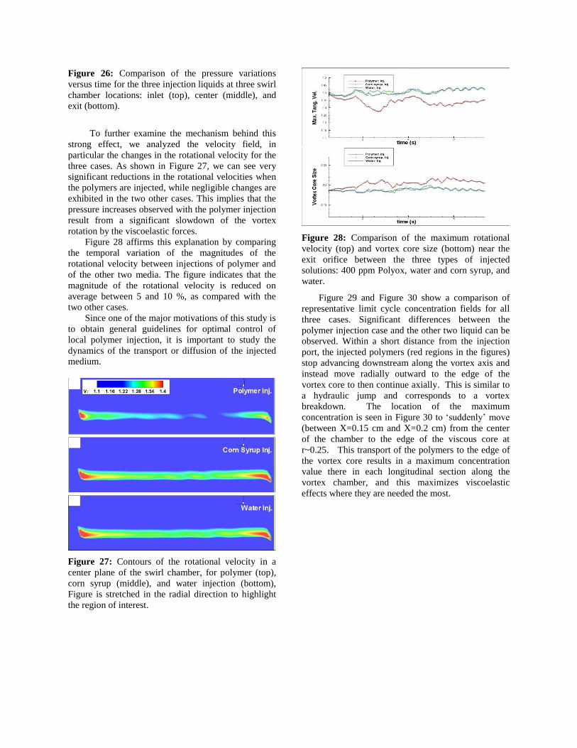
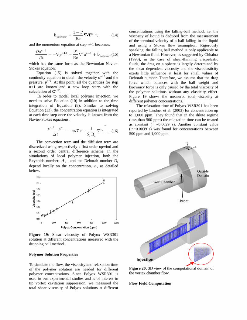
Figure 26: Comparison of the pressure variations

versus time for the three injection liquids at three swirl

chamber locations: inlet (top), center (middle), and

exit (bottom).

To further examine the mechanism behind this

strong effect, we analyzed the velocity field, in

particular the changes in the rotational velocity for the

three cases. As shown in Figure 27, we can see very

significant reductions in the rotational velocities when

the polymers are injected, while negligible changes are

exhibited in the two other cases. This implies that the

pressure increases observed with the polymer injection

result from a significant slowdown of the vortex

rotation by the viscoelastic forces.

Figure 28 affirms this explanation by comparing

the temporal variation of the magnitudes of the

rotational velocity between injections of polymer and

of the other two media. The figure indicates that the

magnitude of the rotational velocity is reduced on

average between 5 and 10 %, as compared with the

two other cases.

Since one of the major motivations of this study is

to obtain general guidelines for optimal control of

local polymer injection, it is important to study the

dynamics of the transport or diffusion of the injected

medium.

Figure 27: Contours of the rotational velocity in a

center plane of the swirl chamber, for polymer (top),

corn syrup (middle), and water injection (bottom),

Figure is stretched in the radial direction to highlight

the region of interest.

Figure 28: Comparison of the maximum rotational

velocity (top) and vortex core size (bottom) near the

exit orifice between the three types of injected

solutions: 400 ppm Polyox, water and corn syrup, and

water.

Figure 29 and Figure 30 show a comparison of

representative limit cycle concentration fields for all

three cases. Significant differences between the

polymer injection case and the other two liquid can be

observed. Within a short distance from the injection

port, the injected polymers (red regions in the figures)

stop advancing downstream along the vortex axis and

instead move radially outward to the edge of the

vortex core to then continue axially. This is similar to

a hydraulic jump and corresponds to a vortex

breakdown. The location of the maximum

concentration is seen in Figure 30 to ‘suddenly’ move

(between X=0.15 cm and X=0.2 cm) from the center

of the chamber to the edge of the viscous core at

r~0.25. This transport of the polymers to the edge of

the vortex core results in a maximum concentration

value there in each longitudinal section along the

vortex chamber, and this maximizes viscoelastic

effects where they are needed the most.

Figure 29: Contours of the injection mass

concentration along the vortex chamber longitudinal

direction for injection of polymers (top), corn syrup

solution (middle), and water (bottom). The scale is

stretched in the radial direction to expand the region of

interest.

In contrast, in both cases of injecting corn syrup

solution or water, the injected medium tends to

advance in the chamber along the axis first and then

diffuse gradually to the edge of the core. The jump of

the location of the maximum concentration (vortex

breakdown) also occurs but much later (e.g. X~10

cm), i.e. at 10 times the distance required by the

polymers.

Figure 30: Comparison of the concentrations along

the chamber axis for the three injected media (top).

Radial location of the maximum concentration for the

three injected media (bottom).

This can be clearly visualized by considering the

axial velocities and pressure distributions along the

axis of the chamber as illustrated in Figure 31. It is

seen that the pressures increase along the axis for the

polymer injection case and result in a reverse axial

flow in the vortex which drives the polymers to move

more towards the edge of vortex core, rather than stay

at the core center. All these are consistent with our

flow visualization using dye shown in the earlier

sections.

Figure 31: Comparison of the axial velocities for the

three injected media (Top). Comparison of the

pressure coefficients for the three injected media

(Bottom).

Interpretation - Stress Tensor

In classical simple shear viscoelastic flows, non-zero

diagonal terms are the consequence of the polymer

molecule stretching along shear direction; here the

vortex axis and the azimuthal directions. The off-

diagonal components, such as xT is proportional to

the product of the two major shear rate components

and contributes to the flow as an effective strong

friction force to slow down the vortex rotation. Kumar

and Homsy (1999) and Yu and Phan-Thien (2004)

studied the roll-up of a free shear layer in a

viscoelastic liquid and found that the roll-up process is

suppressed by the normal stress component such

as, T the vortex chamber problem. Though the

problem studied here has axial variation which

vanishes in the quasi-steady solutions in these studies,

the mechanisms for the rotation slow-down are the

same.

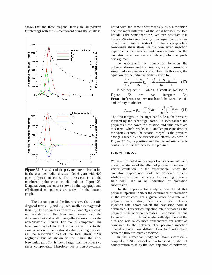
Figure 32 shows a snapshot of a typical radial

distribution of the various components of the polymer

stress tensor at the monitored point near the chamber

exit shown in Figure 23. The top part of the figure

shows that the three diagonal terms are all positive

(stretching) with the Trr component being the smallest.

Figure 32: Snapshot of the polymer stress distribution

in the chamber radial direction for 6 gpm with 400

ppm polymer injection. The cross-cut is at the

monitored point close to the exit in Figure 23.

Diagonal components are shown in the top graph and

off-diagonal components are shown in the bottom

graph.

The bottom part of the figure shows that the off-

diagonal terms, Txr and Tr , are smaller in magnitude

than Tx.. The polymer extra stress Txr and Tr are close

in magnitude to the Newtonian stress with the

difference that a shear-thinning effect shows up for the

non-Newtonian liquids. For the x component, the

Newtonian part of the total stress is small due to the

slow variation of the rotational velocity along the axis,

i.e. the Newtonian part of the total stress x is

negligible but as shown in the figure the non-

Newtonian part Tx is much larger than the other two

shear components. Therefore, for a non-Newtonian

liquid with the same shear viscosity as a Newtonian

one, the main difference of the stress between the two

liquids is the component x . We thus postulate it is

the non-Newtonian stress Tx that significantly slows

down the rotation instead of the corresponding

Newtonian shear stress. In the corn syrup injection

experiments, the shear viscosity was increased but the

cavitation inception was not delayed, which supports

our argument.

To understand the connection between the

polymer stresses and the pressure, we can consider a

simplified axisymmetric vortex flow. In this case, the

equation for the radial velocity is given by: 2

1 1

Re Re

rrrr

u T Tp T

r r r

(17)

If we neglect rrT , which is small as we see in

Figure 32, we can integrate Eq.

Error! Reference source not found. between the axis

and infinity to obtain: 2

0 0

1

Revortex

u Tp p dr dr

r r

(18)

The first integral in the right hand side is the pressure

induced by the centrifugal force. As seen earlier, the

polymers slow down the rotation and thus attenuate

this term, which results in a smaller pressure drop at

the vortex center. The second integral is the pressure

change caused by the viscoelastic effects. As seen in

Figure 32, T is positive and the viscoelastic effects

contribute to further increase the pressure.

CONCLUSIONS

We have presented in this paper both experimental and

numerical studies of the effect of polymer injection on

vortex cavitation. In the experimental study, the

cavitation suppression could be observed directly

while in the numerical study the resulting pressure

field was used as an indication of cavitation

suppression.

In the experimental study it was found that

polymer injection inhibits the occurrence of cavitation

in the vortex core. For a given water flow rate and

polymer concentration, there is a critical polymer

injection rate above which the cavitation core is

eliminated. This critical injection rate decreases as the

polymer concentration increases. Flow visualizations

for injections of different media with dye showed the

diffusion was much more concentrated for water as

compared to the polymer. The polymer injection

created a much more diffused flow field with much

scattered flow structures observed.

In the numerical study we have successfully

coupled a FENE-P model with a transport equation of

concentration to study the local injection of polymers,

corn syrup water solution, and water in the swirl

chamber. It was found that the injection of polymers

reduces the rotational velocity and increases the

pressure along the vortex while injection of the other

two liquids has a negligible effect at the same injection

flow rate. Detailed analysis of the injected liquid

concentration explained the mechanism which caused

the dye to diffuse more around the vortex core edge in

our flow visualization with dye. This appears to be

related to a vortex breakdown following polymer

injection, which occurs much earlier with the

viscoelastic polymers. This results in slowing down of

the rotation velocity and attenuation of the centrifugal

force. This, as well as the existence of additional

viscoelastic stresses, results in higher pressures at the

vortex center.

ACKNOWLEDGMNETS This work was conducted at DYNAFLOW, INC.

(www.dynaflow-inc.com) under support from the

Office of Naval Research, Contract No. N00014-08-C-

0448 monitored by Dr. Ki-Han Kim. We thankfully

acknowledge this support.

REFERENCES

Arabshahi, A., Taylor, L.K., Whitfield, D.L.,

“UNCLE: Toward a Comprehensive Time Accurate

Incompressible Navier-Stokes Flow Solver, AIAA-95-

0050, 1995.

Barbier, C. and Chahine, G.L., “Experimental Study

on the Effects of Viscosity and Viscoelasticity on a

Line Vortex Cavitation”, Proceedings of the 7th

International Symposium on Cavitation, CAV2009,

Ann Arbor, Michigan, 2009.

Bird, R.B. Armstrong, R.C., and Hassager, O.,

Dynamics of Polymeric Liquids, vol. 1&2, Wiley,

New York, 1987.

Chahine, G.L., Frederick, G.F. and Bateman, R.D.,

“Propeller Tip Vortex Cavitation Suppression Using

Selective Polymer Injection”, J. Fluids Engr., Vol.

115, pp.497-503, 1993.

Chhabra, R.P., Drops, and Particles in Non-Newtonian

Fluids, CRC Press, Boca Raton, FL, 1993.

Chorin, A. J., “A Numerical Method for Solving

Incompressible Viscous Flow Problems,” Journal of

Computational Physics, Vol. 2, pp. 12-26, 1967.

Fruman, D. and Aflalo, S., “Tip Vortex Cavitation

Inhibition by Drag Reducing Polymer Solution”, J.

Fluids Engr. Vol. 111, pp.211-216, 1989.

Fruman, D.H., Pichon, T. and Cerrutti, P., “Effect of a

Drag-reducing Polymer Solution Ejection on Tip

Vortex Cavitation”, J. Mar. Sci. Tech., Vol. 1, pp.13-

23, 1995.

Hsiao, C-T. Zhang, Q., Wu, X. and Chahine, G.L.,

“Effects of Polymer Injection on Vortex Cavitation

Inception”, 28th

Naval Hydrodynamics Symposium,

Pasadena, CA. 17-22, Sep. 2009.

Kumar, S. and Homsy, G.M., “Direct numerical

simulation of hydrodynamic instabilities in two- and

three-dimensional viscoelastic free shear layers”,

Journal of Non-Newtonian Fluid Mechanics, 83,

pp249-276, 1999.

Latorre, R., Muller, A., Billard, J.Y. and Houlier, A.,

“Investigation of the Role of Polymer on the Delay of

Tip Vortex Cavitation”, J. Fluids Engr., Vol. 126,

pp.724-729, 2004.

Li, C.F., Sureshkumar, R. and Khomami, B.,

“Influence of Rheological Parameters on Polymer

Induced Turbulent Drag Reduction”, J. Non-

Newtonian Fluid Mech. Vol. 140, pp23-40, 2006.

Lindner, A., Vermant, J. and Bonn, D., “How to

Obtain the Elongational Viscosity of Dilute Polymer

Solutions”, Physica A, Vol. 319, pp.125-133, 2003.

Platzer G.P. and Souders W.G. “Tip Vortex Cavitation

Delay with Application to Marine Lifting Surfaces. A

literature Survey,” DTNSRDC Technical Report

79/051, 1979.

Chang, N., Ganesh, H., Yakushiji, R., Ceccio, S.L.,

“Tip Vortex Cavitation Suppression by Active Mass

Injection”, J. of Fluids Eng. Vol. 133 (11), 111301,

2011.

Roe, P. L., “Approximate Riemann Solvers, Parameter

Vectors, and Difference Schemes,” Journal of

Computational Physics, 43, pp. 357-372, 1981.

van Leer, B., “A Second Order Sequel to Godunov's

Method”, J. Comp. Phys., 32, pp. 101–136, 1979.

Yu, Z. and Phan-Thien, N., “ Three-dimenional roll-up

of a viscoelastic mixing layer ”, Journal of Fluid

Mechanics, 500, pp29-53, 2004.

Zhang, Q., Hsiao, C-T. and Chahine, G.L., “Numerical

Study of Vortex Cavitation Suppression with Polymer

Injection”, Proceedings of the 7th

International

Symposyum on Cavitation, Aug 17-22, Ann Arbor,

Michigan , 2009.