Volume Rendering - LSU

B. B. Karki, LSUCSC 7443: Scientific Information Visualization

Volume Rendering


Volume Rendering versus Other Techniques

• Volume rendering: creates a 2D image directly from 3Dvolumetric data Mapping the entire 3D data into a 2D image Volume images retain full information at the cost of increased

algorithm complexity and rendering times Rendering of amorphous phenomena such as clouds, fog

• Surface rendering: creates an image of a surface containedwithin the volume data using geometric primitives Triangles or points

• Clipping: removes a part of a volume to display the rest of thecontents Applicable with volume or surface rendering.


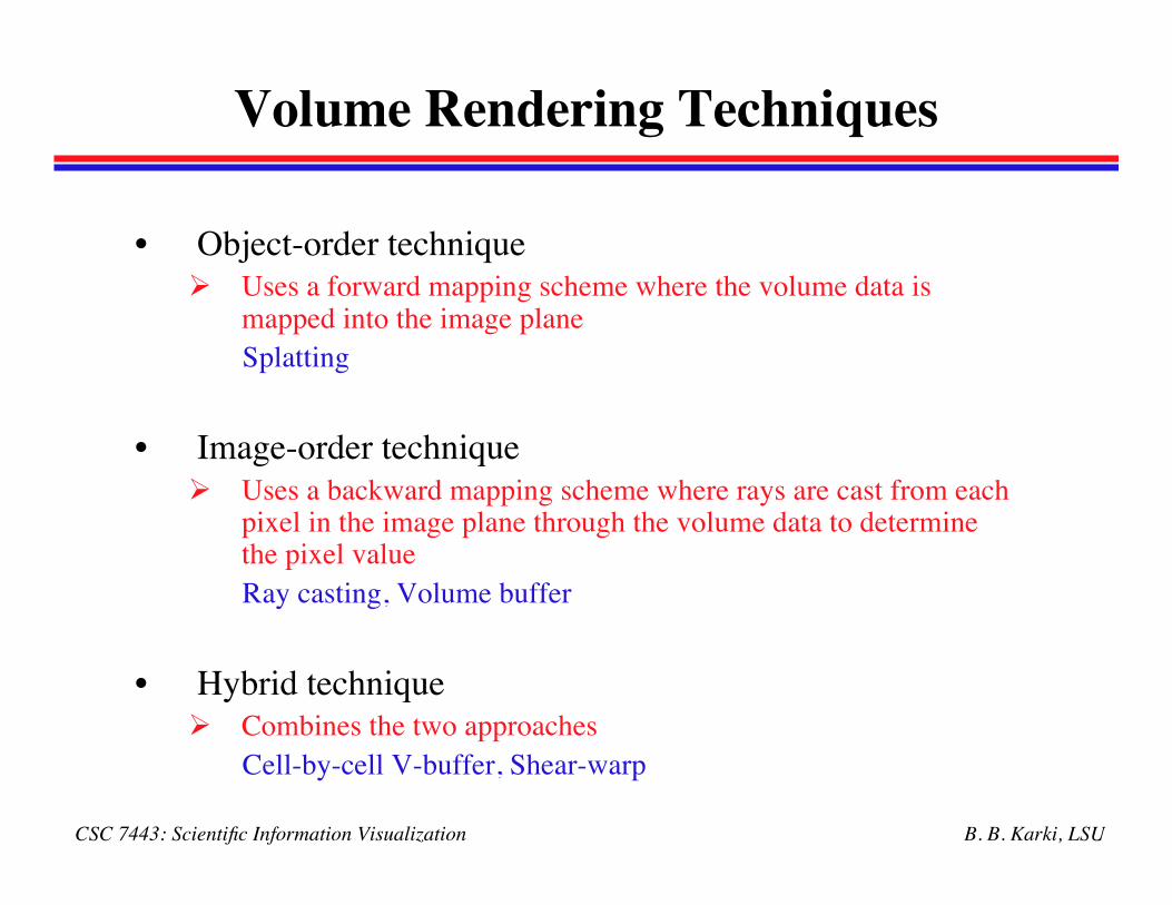
Volume Rendering Techniques

• Object-order technique Uses a forward mapping scheme where the volume data is

mapped into the image plane Splatting

• Image-order technique Uses a backward mapping scheme where rays are cast from each

pixel in the image plane through the volume data to determinethe pixel value Ray casting, Volume buffer

• Hybrid technique Combines the two approaches

Cell-by-cell V-buffer, Shear-warp


Splatting


What is Splatting?

• Object-order rendering: Forward mapping algorithm that mapsdata samples onto the image plane

• Splatting considers how a sample can contribute to many pointsin space, and hence to many pixels in the image plane in termsof a distribution function Distributes energy from input samples into space Calculates an image plane footprint for each data sample and uses the

footprint to spread the sample’s energy onto the image plane Works for regular grid with/out the same spacings in all directions Can be parallel.

L. Westover, Footprint evaluation for volume rendering, Computer Graphics, vol 24, no. 4, August 1990


Basic Four Steps

• Transforming sample from input <i,j,k> grid space to <x,y,z> screen space

• Shading sample using some shading rule: <x,y,z,R,G,B,A>

• Reconstruction step: Determine the portion of the image the sample can affect andadd the sample’s contribution to the sheet accumulator Defining and computing footprint function Every data sample is convolved with a reconstruction kernel to produce the

image of this data sample.

• Visibility: Matt the sheet accumulator to the working image using a compositingoperator when all samples that lie in a sheet are processed

• Once all samples are processed, the working image becomes the final image.


Contribution of a Voxel to Image Plane

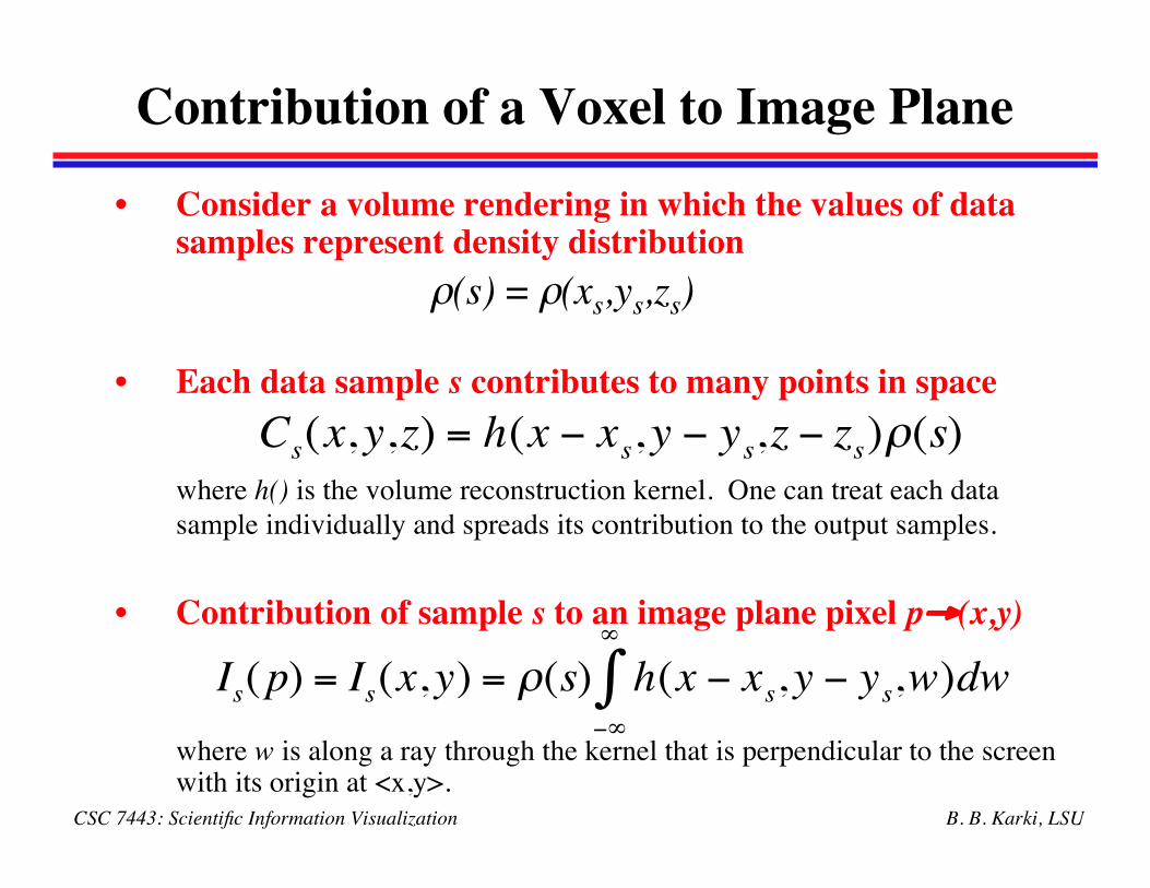
• Each data sample s contributes to many points in space

!

Cs(x,y,z) = h(x " xs,y " ys,z " zs)#(s)where h() is the volume reconstruction kernel. One can treat each datasample individually and spreads its contribution to the output samples.

• Consider a volume rendering in which the values of datasamples represent density distribution ρ(s) = ρ(xs,ys,zs)

!

Is(p) = Is(x,y) = "(s) h(x # xs,y # ys,w)dw#$

$

%• Contribution of sample s to an image plane pixel p→(x,y)

where w is along a ray through the kernel that is perpendicular to the screenwith its origin at <x,y>.


Splat Footprint

!

Is(p) = "(s)F(x # xs,y # ys)

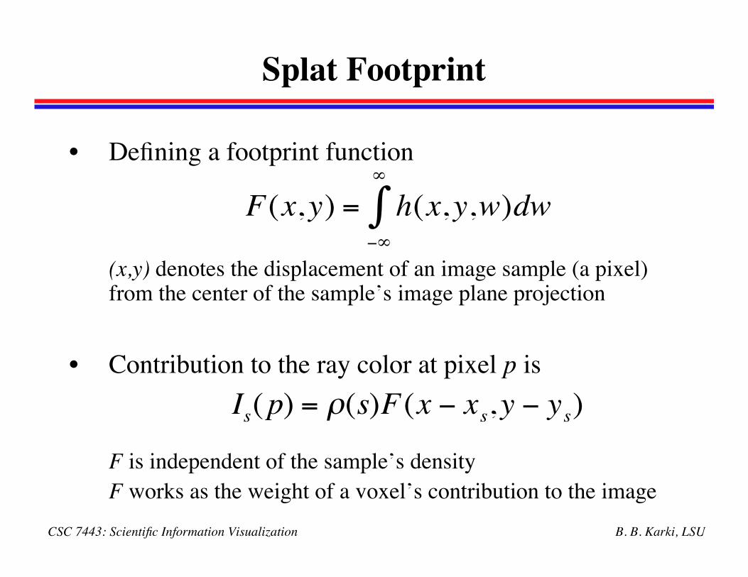
• Defining a footprint function

!

F(x,y) = h(x,y,w)dw"#

#

$

F is independent of the sample’s densityF works as the weight of a voxel’s contribution to the image

• Contribution to the ray color at pixel p is

(x,y) denotes the displacement of an image sample (a pixel)from the center of the sample’s image plane projection


Total Contribution

!

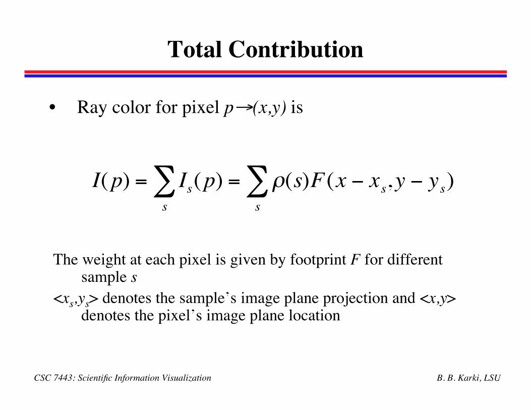
I(p) = Is(p)s

" = #(s)F(x $ xs,y $ ys)s

"

• Ray color for pixel p→(x,y) is

The weight at each pixel is given by footprint F for differentsample s

<xs,ys> denotes the sample’s image plane projection and <x,y>denotes the pixel’s image plane location


Reconstruction Kernel

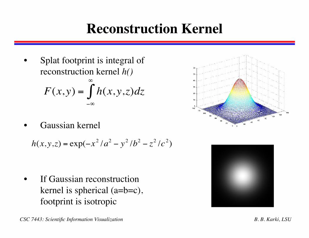
• Splat footprint is integral ofreconstruction kernel h()

• Gaussian kernel

• If Gaussian reconstructionkernel is spherical (a=b=c),footprint is isotropic

!

F(x,y) = h(x,y,z)dz"#

#

$

!

h(x,y,z) = exp("x2/a

2" y

2/b

2" z

2/c

2)


Footprint Table

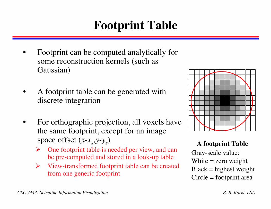
• Footprint can be computed analytically forsome reconstruction kernels (such asGaussian)

• A footprint table can be generated withdiscrete integration

• For orthographic projection, all voxels havethe same footprint, except for an imagespace offset (x-xs,y-ys) One footprint table is needed per view, and can

be pre-computed and stored in a look-up table View-transformed footprint table can be created

from one generic footprint

A footprint TableGray-scale value:White = zero weightBlack = highest weightCircle = footprint area


View-Transformed Footprint Table

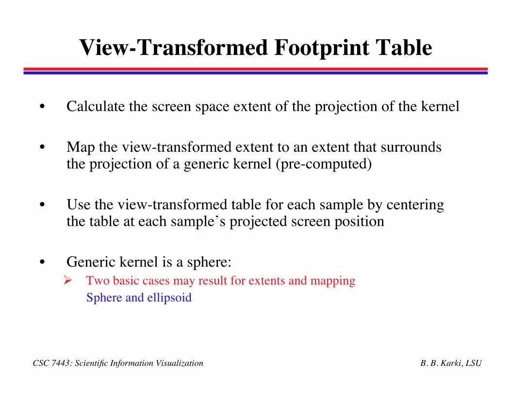
• Calculate the screen space extent of the projection of the kernel

• Map the view-transformed extent to an extent that surroundsthe projection of a generic kernel (pre-computed)

• Use the view-transformed table for each sample by centeringthe table at each sample’s projected screen position

• Generic kernel is a sphere: Two basic cases may result for extents and mapping

Sphere and ellipsoid


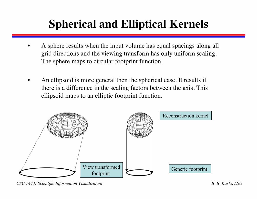
Spherical and Elliptical Kernels• A sphere results when the input volume has equal spacings along all

grid directions and the viewing transform has only uniform scaling.The sphere maps to circular footprint function.

• An ellipsoid is more general then the spherical case. It results ifthere is a difference in the scaling factors between the axis. Thisellipsoid maps to an elliptic footprint function.

Generic footprint

Reconstruction kernel

View transformedfootprint


Extent and Mapping

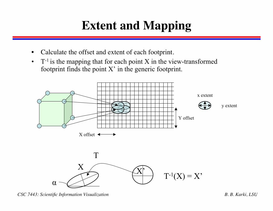
• Calculate the offset and extent of each footprint.• T-1 is the mapping that for each point X in the view-transformed

footprint finds the point X’ in the generic footprint.

x extent

y extent

X offset

Y offset

T

X’XT-1(X) = X’

α


The Graphics Pipeline

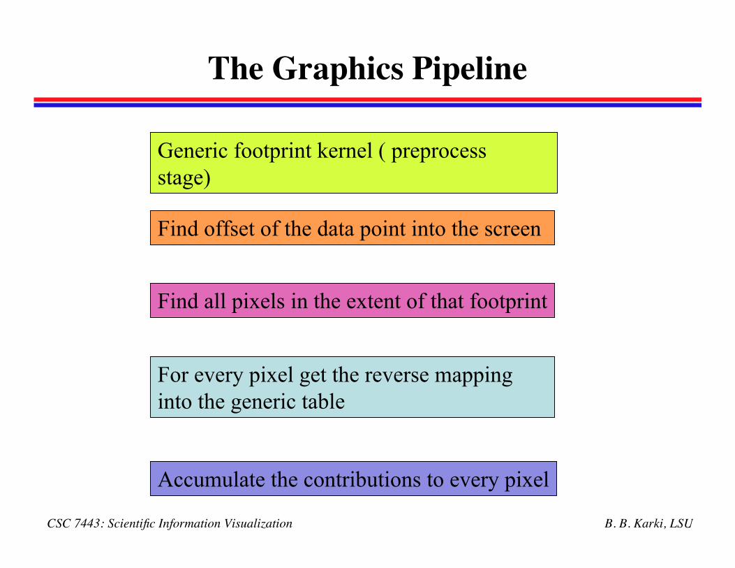
Generic footprint kernel ( preprocessstage)

Find offset of the data point into the screen

Find all pixels in the extent of that footprint

For every pixel get the reverse mappinginto the generic table

Accumulate the contributions to every pixel


Subsequent Developments

• The basic splatting algorithm was refined by more recent work.

• K. Mueller et al., High quality splatting on rectangular grids with efficient culling ofoccluded voxels – IEEE Trans. on Visualization and Computer Graphics, 1999.

• J. Huang et al. FastSplats: Optimized splatting on rectilinear grids, FastSplats: Optimized splatting on rectilinear grids, IEEE Visualization'00, Salt-LakeCity, October 2000

• N. Neophytou and K. Mueller, Space-time points: 4D Splatting on efficient grids,Symposium on Volume Visualization and Graphics 2002, Boston, October 2002

• N. Neophytou and K. Mueller, Post-convolved splatting, Joint Eurographics - IEEETCVG Symposium on Visualization 2003, Grenoble, France, May 2003


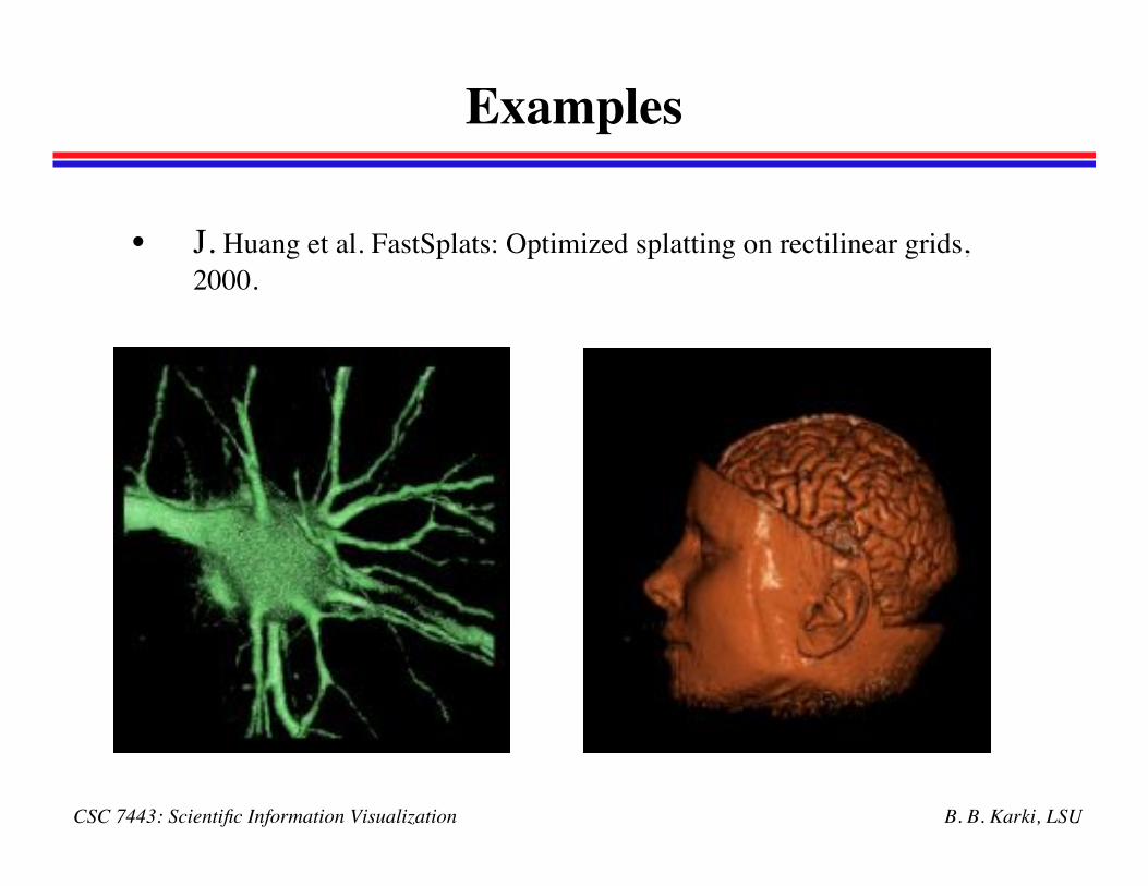
Examples

• J. Huang et al. FastSplats: Optimized splatting on rectilinear grids,2000.

Documents

Volume Rendering - LSU