Volume I: Applied Probability

C.C. HeydeYu V. Prohorov

R.PykeS.T. Rachev

(Editors)

Athens Conference on Applied Probabilityand Time Series Analysis

Volume I: Applied ProbabilityIn Honor of J.M. Gani

398 Statistical Models op Earthquake Occurrence

Printed: December 4, 1995

PROBLEMS IN THE MODELLING AND

STATISTICAL ANALYSIS OF EARTHQUAKES

Y. Y. Kagan1 and D. Vere-Jones2

1Institute ofGeophysics and Planetary Physics, University ofCalifornia, Los Angeles, California90095-1567, USA. (E-mail: [email protected])

2Institute ofStatistics and Operations Research, Victoria University of Wellington, P.O. Box600, Wellington, New Zealand. (E-mail: [email protected])

1. INTRODUCTION

The purpose of this paper is to set out some of the statistical and probabilistic problems thatarise from the work of the first author over the past two decades. Nearly all of this work hasbeen published in geophysical journals, where themajor emphasis is on the physical interpretationof the model structure and subsequent statistical analysis. One consequence is that many of themathematical issues inherent in themodel structures and conceptions have never been fully explored(see also Vere-Jones, 1994). In fact they raise many issues for discussion, from the adequacyof existing stochastic models for processes exhibiting self-similar or fractal behaviour, to specificquestions concerning the testing of statistical models for random 3-dimensional rotations. Ourhope is that by reviewing these papers in the context ofthe present conference, we may encourageattempts to resolve some of the more mathematicalissues which arise, or relate them to relevantrecent work.

The work under review can be roughly divided into three phases. The first phase, includingpapers K1-K4 (seereference section), dates to the early 1980's and was concerned with the momentstructure of earthquake spatial locations. The thrust of the work was to expose the basic self-similarity of the earthquake process. There is a broad indication that for k = 2, 3 and 4, theprobability density for thedistribution ofk points selected at random from the catalogue is inverselyproportional to the 'volume' of the minimal convex set spanned by the k points in question. Theunderlying question here is, what sort of models, if any, exhibit these general features? This firstphase is reviewed in section 2.

The second phase relates to Kagan's attempts, outlined in K5 and K6 in particular, to developsimulation models which would comprehensively mirror the above and related features of the observed catalogue data. Here the viewpoint taken is that the crust is in a process of continualelementary fracturing, and it is the eye of the beholder, rather than any intrinsic feature of theprocess, which selects out large clusters of elementary events and identifies them as earthquakes.The resulting simulation model is very successful in this aim, but it is necessarily complex, eventhough it depends on only a small number offitted parameters. In particular it incorporates three-dimensional rotational effects which give the model a special geometrical character of its own. Asa result it is difficult to relate the statistical features of the simulations to theoretical results on themanydifferent types ofbehaviour possible withspatialbranching processes. The model, and somepreliminary attempts to identify its behaviour in theoretical terms, are described in section 3.

Y. Y. Kagan and D. Vere-Jones 399

At best the simulation model provides a purely kinematic picture of earthquake occurrence. Afirst attempt to introduce dynamical aspects comes with attempts to model statistical aspects ofthe stress field in which earthquakes take place, or the modifications to the existing stress fieldcaused by the occurrence of a new event. Here further geometric questions arise. These are closelyrelated to the description of the fault motion in terms of a "double couple" mechanism (Aki andRichards, 1980), essentially equivalent to a 3-dimensional rotation with additional symmetries. Akey role is played by rotational stable distributions which are the analogues here for the stabledistributions which dominate the earlier discussion of spatial locations. These and related issuesare taken up in section 4, covering the papers K7-K11 in particular.

The paper concludes with a brief listing of the main problems noted in the earlier sections,together with a number of more immediate statistical questions.

2. THE SPATIAL MOMENTS OF EARTHQUAKE CATALOGUES

2.1. Empirical Results

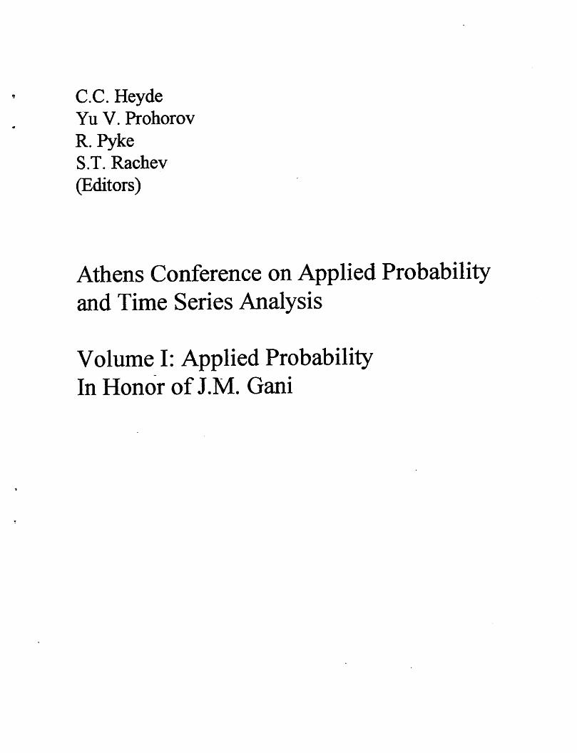
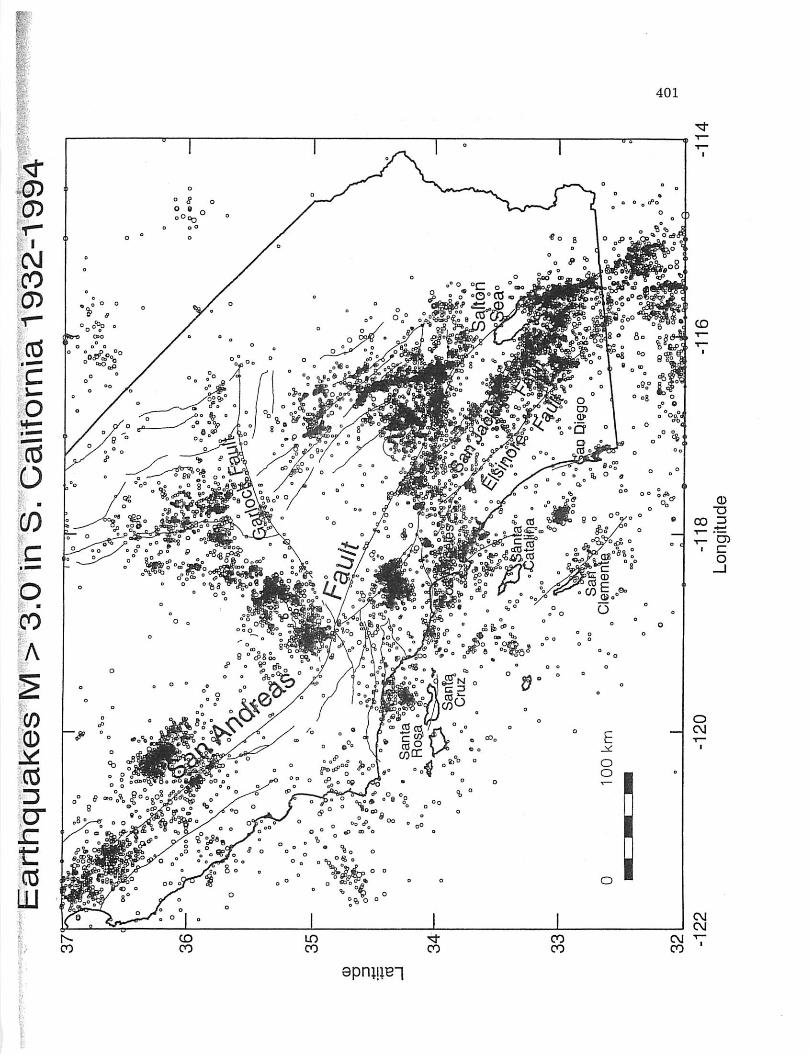
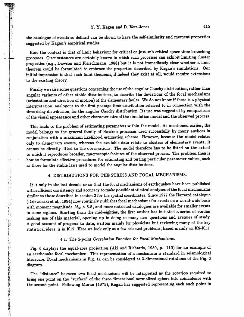
We are concerned here with the catalogue as a list of epicentres (points on the surface of theearth), or hypocentres (points within the earth's crust) of earthquake events identified and locatedwithin a particular geographical region over some stated observational period. The earthquakesize is characterized by the scalar seismic moment (Aki and Richards, 1980), as well as by several'magnitudes' (M), the most important of which is the moment magnitude (Mw), which is basedon measurement of the seismic moment. For historical reasons these magnitudes are adjusted to beclose to-the Richter magnitude. Typical examples of earthquakeepicenter maps are shown in Figs.1(a), 1(b). Catalogues considered range from catalogues of major global events with magnitudesM > 6, regional catalogues from New Zealand or Japan of events with magnitudes M > 4, localcatalogues for selected parts of California with magnitudes M > 1.5. Problems of completeness,accuracy, etc., are discussed in detail in papers K1-K4 and the references therein, and need to becarefully taken into account in the interpretation of any statistical analysis. However we shall leavesuch aspects temporarily aside and just consider the key results, verified for catalogues on a rangeof scales, reported in these four papers.

The first three papers are devoted to studies of the empirical 2-point, 3-point, and 4-point moments of the sets of epicentres and hypocentres (see Fig. 2). The principal quantities studied arethe proportions of k-tuples (k = 2,3,4) of points from the catalogue with the property that themaximum distance between any two points in the A;-tuple does not exceed t , as a function of r,and the joint density function of the coordinates of the points forming such a k-tuple.

Write

ft(r) = Nk(r)/N, (2.1)

where Nk{r) is the number of k-tuples with the stated property, and Nk is the total number ofife-tuples from the catalogue. The quantities qk{f) are computed first for the epicentres, as pointsin R2 , and then for the hypocentres, as points in Rz. As with Ripley's fc-function (Ripley, 1977),they can be interpreted as the average number of k-tuples within a distance r of an "average"point of the catalogue.

In order to overcome the biases in such estimates which come from boundary effects (see e.g.Ripley, 1977; Stoyan et al., 1987; Stoyan and Stoyan, 1994 for details), the above ratios were then

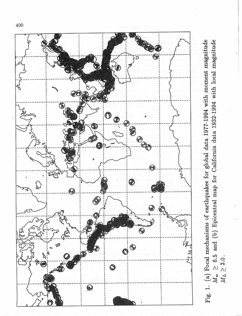
Fig-

1-(a

)Fo

calm

echa

nism

sof

earth

quak

esfo

rgl

obal

data

1977

-199

4w

ithm

omen

tmag

nitu

deM

w>

6.5

and

(b)

Epi

cent

ral

map

for

Cal

iforn

iada

ta19

32-1

994

with

loca

lm

agni

tude

ML

>3

.0.

4^

O O

'

CD

-o ZJ

•♦—»

"♦—»

Eart

hq

uak

es

M>

3.0

inS

.C

ali

forn

ia1

93

2-1

99

4

-11

8

Lon

gitu

de

o

-11

4


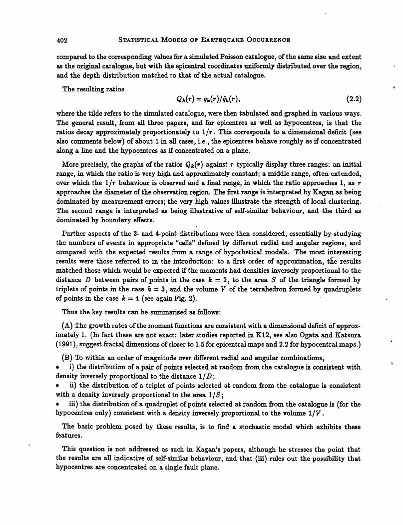
compared to the corresponding values for a simulated Poisson catalogue, of the same size and extentas the original catalogue, but with the epicentral coordinates uniformly distributed over the region,and the depth distribution matched to that of the actual catalogue.

The resulting ratios

Qk(r) = ft(r)/ft(r), (2.2)

where the tilde refers to the simulated catalogue, were then tabulated and graphed in various ways.The general result, from all three papers, and for epicentres as well as hypocentres, is that theratios decay approximately proportionately to 1/r. This corresponds to a dimensional deficit (seealso comments below) of about 1 in all cases, i.e., the epicentres behave roughly as if concentratedalong a line and the hypocentres as if concentrated on a plane.

More precisely, the graphs of the ratios Qfc(r) against r typically display three ranges: an initialrange, in which the ratio is very high and approximately constant; a middle range, often extended,over which the 1/r behaviour is observed and a final range, in which the ratio approaches 1, as rapproaches the diameter of the observation region. The first range is interpreted by Kagan as beingdominated by measurement errors; the very high values illustrate the strength of local clustering.The second range is interpreted as being illustrative of self-similar behaviour, and the third asdominated by boundary effects.

Further aspects of the 3- and 4-point distributions were then considered, essentially by studyingthe numbers of events in appropriate "cells" defined by different radial and angular regions, andcompared with the expected results from a range of hypothetical models. The most interestingresults were those referred to in the introduction: to a first order of approximation, the resultsmatched those which would be expected if the moments had densities inversely proportional to thedistance D between pairs of points in the case k = 2, to the area S of the triangle formed bytriplets of points in the case k = 3, and the volume V of the tetrahedron formed by quadrupletsof points in the case k = 4 (see again Fig. 2).

Thus the key results can be summarized as follows:

(A) The growth rates of the moment functions are consistent with a dimensional deficit of approximately 1. (In fact these are not exact: later studies reported in K12, see also Ogata and Katsura(1991),suggest fractal dimensions of closer to 1.5for epicentralmaps and 2.2for hypocentral maps.)

(B) To within an order of magnitude over different radial and angular combinations,• i) the distribution of a pair of points selected at random from the catalogue is consistent withdensity inversely proportional to the distance l/D;• ii) the distribution of a triplet of points selected at random from the catalogue is consistentwith a density inversely proportional to the area 1/5;• iii) the distribution of a quadruplet of points selected at random from the catalogueis (for thehypocentres only) consistent with a density inversely proportional to the volume 1/V.

The basic problem posed by these results, is to find a stochastic model which exhibits thesefeatures.

This question is not addressed as such in Kagan's papers, although he stresses the point thatthe results are all indicative of self-similar behaviour, and that (iii) rules out the possibility thathypocentres are concentrated on a single fault plane.

i

ft

II

i

isA.

i

Moment

Function

D

Distribution

Density

1/D

1/S

1/V

Fig. 2. Schematic representation of 2-, 3-, and 4-point momentfunctions and their suggested densities.

403

404 Y. Y. Kagan and D. Vere-Jones

2.2. Modelling Considerations

To expose some ofthe issues involved intrying tofind an answer to the above problems, considerfirst the expected value of the quantity N2(r) arising in the definition of q2{r). If we adopt astandard point process notation (see Daley and Vere-Jones, 1988) and assume that the first andsecond moment measures exist, thenwe can write (ignoring boundary effects)

E[N2(r)]= f Ml(dx)Mi(Sr(x)\x), (2.3)Jw

where Mi(dx) = E[N{dx)] is the first moment measure, Mi{dy\x) = E[N(dy)\N(dx) = 1] is thefirst order Palm moment measure, W is the observation region, and Sr(x) is the "sphere" radiusr, centre x.

We see that the behaviour of E[N2(r)] depends both on the character of M\(dx) and on thelocal clustering structure described by M\(dy\x).

In the case of a homogeneous process, with mean density m, Mi(dx) = mdx and M\(dy\x)approaches mdy for large values ofthe distance y-x.m this case E[N2(r)] will ultimately growas rd, where d is the dimension ofthe space under study. This means that theratios Q2(r) will beasymptotically constant for large r, and will not therefore exhibit the inverse power law behaviourthat is claimed.

A number of ways can be suggested to get around this apparent difficulty: the power law behaviour-may relate to the correlations rather than the moments; the point process may be "Palm-homogeneous" (see definition below) rather than strictly homogeneous; or the observed behaviourmayreflect purely the properties of M\(dx), as in a Poisson process with singular parameter measure. We explore each of these possibilities briefly below. In none of these, however, does an easyanswer to the basic question seem available. We remain uncertain, therefore, whether or not apoint process model can be defined which exhibits the basic features A, B claimed by Kagan forthe empirical earthquake data.

(a) Power law correlations with a homogenous model

The covariance measure for a point process model can be defined by

C2(dx x dy) = E[dN(x)dN(y)) - E[dN(x)]E[dN(y)]. (2.4)

In the homogenous case, and assuming derivatives exist, this can be simplified to

C2(y - x) = m[mi(y\x) - m], (2.5)

where the Palm intensity mi(y\x) is also a function of y - x only. In the earthquake applications,TOi(y|*) >> m for y - x small, and it is a matter of indifference, and probably impossible todetermine from a finite data set, whether the power decay relates to mi(y\x) directly, or to thedifference mi(y\x)-m. By taking the latter point ofview, as inthe studies byVere-Jones (1978) andChong (1983), one can remain formally within the context ofspatially homogeneous processes, yetstill retain approximate power-law behaviour for the second moment measure, and an appearanceof self-similarity.

¥

vg Statistical Models op Earthquake Occurrence 405:&.

;!? An approach of this kind has been taken recently by Stoyan (1994), in part to emphasize the| care that needs to be takenin distinguishing point process models that have non-standard fractal

dimension from those which exhibit self-similarity. Roughly speaking, the correlation dimensionof a point process model can be defined as the limit of the ratio of logE(N2(r)/log(r)) as r

T approaches zero. Non-standard dimensions can be achieved even for such a simple example asthe Neyman-Scott model by choosing a sufficiently irregular form for mi{y\r). However, strictself-siniilarity is not possible for a point process model as usually defined, since it requires infiniteaccumulations of points in bounded regions; still less can it be achieved for a homogeneous model,which implies the existence of a mean distance between points, and hence a distinguished distance

- scale. The situation if the process is non-homogeneous is not so clear. The assumption of finite• moment measures, required to ensure the existence of the quantities appearing in the definition of

the fractal dimension, does not of itself rule out self-similarity, at least in an approximate sense.However, if appropriate examples exist, they are elusive.

\: Unfortunatelyit appears to be self-similarity, rather than an anomalous fractal dimensionas such,1 which characterises the earthquake process. Moreover it becomes increasingly difficult to match| the behaviour ofany model to the apparent behaviour ofthe higher moments ofthe earthquake} catalogues. To take the 3-point moment for the epicenters as an example, one has to find a momentj£._ measure which behaves as if it had a density in R2 XR2 proportional to l/RiR2 sin(0), where|<t R\ and #2 are distances between x and y and x and z in a triple (x,y,z), and 0 is the anglej; between the lines (a:, y) and (x,z). The radial factors integrate out, but the term in sin 0 producesi.: a singularity which cannot be integrated out: there is too great a concentration on long skinnym triangles. The situation is even worse for the four-point moments. For the hypocentres, the function' (l/RiR2 sin0), considered now as a function in R3 x Rz, is integrable at zero, and is therefore

\f- a conceivable candidate for a density. On the other hand the 1/V form for the 4-point moment;;: density again gives rise to a singularity. Thus the inverse area and inverse volume properties forceI•; one either to reject the model for sufficiently small angles in the configuration, or to seek a modelf outside the framework of point processes with absolutely continuous factorial moment or cumulant|| measures.

jV From a physical point of view it is ofcourse true that the observed behaviour ultimately breaksj':> down as one reaches the scale of individual rock grains, or certainly individual molecules or atoms.'j If one accepts this limitation, the problem is to find a cluster structure with the right form of power

law behaviour over at least a very extended range. We pick up this problem below in a slightly*Wi wider context.ifj& (b) Palm-stationary point processes

|( Kagan refers at several points to the suggestion ofMandelbrot (1983) that point process models& for self-similar behaviour should be sought not within the class of homogeneous processes but withinI*;; the class ofprocesses for which the behaviour relative to a given point oftheprocess is independent

of the point selected as origin.\%

!£•'.•

it\<si

One interpretation of this requirement is that the Palm distributions of the process should be thesame for all points of the process. This would imply in particular that the moment measures of thePalm distributions were functions of the differences between the arguments only, for example, thatMi{dy/x) was again a function of y —x only, even though the process was not itself homogeneous.We shall refer to such processes as Palm-stationary point processes. In the 1-dimensional case they


correspond to processes which are interval-stationary but not necessarily stationary.

Examples of such Palm-stationary point processes include the random walk (or "random flight")examples of Mandelbrot (1975). Mandelbrot shows that by choosing the step-length to have aPareto distribution, processes can be found for which

rmiSrWl*)** (2.6)

Note that Mandelbrot's distributions are truncated near r = 0, so the power law behaviour doesnot persist for indefinitely small values of r. For larger values of r, however, they exhibit manyproperties of self-similarity.

Unfortunately, according to Kagan (K3), they do not exhibit the higher moment properties ofthe earthquake process, in particular the 1/V property of the four-point moment function. It ispossible, however, that more complex examples could do so. Indeed, the branching process modelsconsidered in section 3 could well include examples of this type.

What hampers us in pursuing this discussion, is that we are not aware of a well establishedtheory for such Palm-stationary point processes. For example, given a candidate family of Palmdistributions, when does there exist a well-defined point process with these distributions? And isthat point process unique? Any references which deal with these or related questions would beappreciated.

Further examples of Palm-stationary processes suggested by Mandelbrot, such as the Levy dustmodel or the zeros of Brownian motion, have a very complexpoint set structure, including finite accumulation points, and cannot therefore be modelled within the standard pointprocess framework.Mandelbrot hints that more general stochastic frameworks could be developed for this purpose,but again we do not know whether any systematic attempts have been made to build up such aframework, nor, if they have, whether they include processes which can match the l/S and 1/Vbehaviour observed by Kagan. Again references would be appreciated.

(c) Singular Poisson processes

Here we consider the opposite type of explanation for the observed behaviour of the momentfunctions to that suggested in (a). For a pure Poisson process there is no cluster structure, sothat M\(dy/x) = M\(dy) = u-(dy) where /x is theparameter measure ofthe process. In this case,therefore

E[N2(r)) = / p[Sr(x))p(dx). (2.7)Jw

Thisshows immediately that the correlation dimension for the point process, interpreted as the limitof the ratio of the logarithm of (2.7) to logr as r approaches zero, coincides with the correlationdimension of the parameter measure p.. The same thing happens also with the higher momentsE(iVfc(r)); after appropriate rescaling they yield inthelimit thek-th order Renyi moment dimensionof \i, defined by

Qk =lim[j3j logJp(Sr)k-lli\dz] Ilogr, (2.8)whenever the limit exists (see, for example, Cutler, 1991; Geilikhman et al., 1990; or Vere-Jones etal., 1995 for further discussions of these dimensions).

w

I

Um

!%

»*_

U

Statistical Models of Earthquake Occurrence 407

Although there are many examples of measures which have fractional moment dimensions, it israther less easy to match the self-similar behaviour of the process to corresponding properties ofp. Well-known examples such as the Cantor measure exhibit scale invariance only with regard toa fixed sequence of scales (in that case powersof 3). Much of the Russian discussion of earthquakeprocesses is couched in the terminology of "hierarchical block structures", where, again, self-similarbehaviour is observed in a sequence of increasing or decreasing scales, but not on all scales.

Once again we are lacking information on whether there has been any attempt to develop a theoryof point process models based on this weaker concept of "intermittent self-similarity". Kagan'sresults do not suggest any such restrictions, but if the point process is to be self-similar at allscales, the underlying measure has to be fully scale invariant, and we already know that for Rd,the only such measures are a product of angular and radial components about a fixed origin, wherethe radial component has density proportional to 1/r. (See the discussion on p. 325 of Daley andVere-Jones, 1988). This type of behaviour seems inappropriate as a model for earthquakes, becauseof its dependence on a fixed origin. Once again the required model seems elusive.

3. THE KAGAN-KNOPOFF BRANCHING MODEL

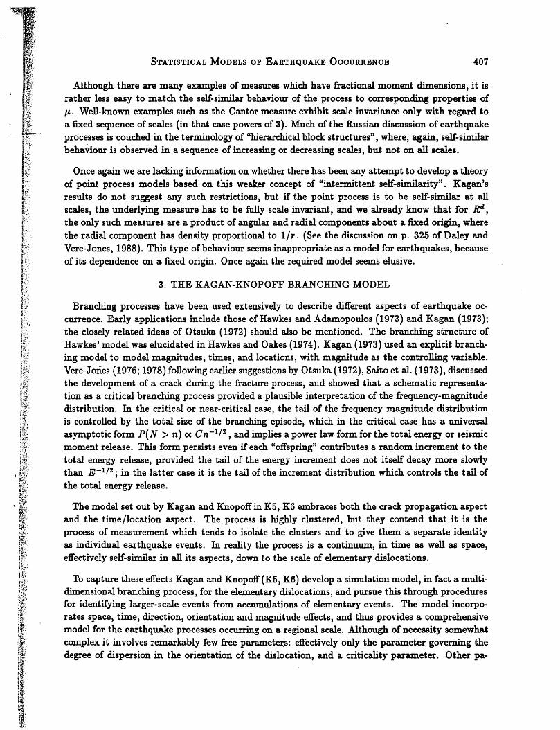
Branching processes have been used extensively to describe different aspects of earthquake occurrence. Early applications include those of Hawkes and Adamopoulos (1973) and Kagan (1973);the closely related ideas of Otsuka (1972) should also be mentioned. The branching structure ofHawkes' model was elucidated in Hawkes and Oakes (1974). Kagan (1973)used an explicit branching model to model magnitudes, times, and locations, with magnitude as the controlling variable.Vere-Jones (1976; 1978)following earliersuggestions by Otsuka (1972), Saito et al. (1973), discussedthe development of a crack during the fracture process, and showed that a schematic representation as a critical branching process provided a plausible interpretation of the frequency-magnitudedistribution. In the critical or near-critical case, the tail of the frequency magnitude distributionis controlled by the total size of the branching episode, which in the critical case has a universalasymptotic form P(N > n) oc Cn~ll2 , andimplies a power law form for the total energy or seismicmoment release. This form persists even if each "offspring" contributes a random increment to thetotal energy release, provided the tail of the energy increment does not itself decay more slowlythan E~1/2; in the latter case it is the tail of the increment distribution which controls the tail ofthe total energy release.

The model set out by Kagan and Knopoff in K5, K6 embraces both the crack propagation aspectand the time/location aspect. The process is highly clustered, but they contend that it is theprocess of measurement which tends to isolate the clusters and to give them a separate identityas individual earthquake events. In reality the process is a continuum, in time as well as space,effectively self-similar in all its aspects, down to the scale of elementary dislocations.

To capture these effects Kagan and Knopoff(K5, K6) develop a simulation model, in fact a multidimensional branching process, for the elementary dislocations, and pursue this through proceduresfor identifying larger-scale events from accumulations of elementary events. The model incorporates space, time, direction, orientation and magnitude effects, and thus provides a comprehensivemodel for the earthquake processes occurring on a regional scale. Although of necessity somewhatcomplex it involves remarkably few free parameters: effectively only the parameter governing thedegree of dispersion in the orientation of the dislocation, and a criticality parameter. Other pa-


rameters are built into the model, and have values suggested on physical grounds and confirmedby further simulation studies.

Despite the interest of the model, and the many questions which it raises, it has not (to ourknowledge) been the subject of any significant analytical investigations. In particular it is notclear how key aspects, such as its evident self-similarity, or the clustering of events subsequentlyidentified as earthquakes, can be deduced from its defining elements. The main purposes of thissection are to briefly summarize the model structure, and to indicate some possible directions forpursuing these questions.

3.1. Description of the Simulation Model

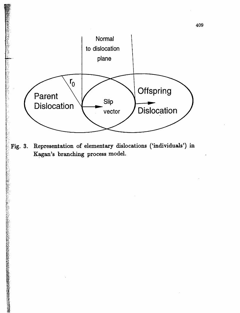
The individuals in the branching process are elementary dislocations, i.e., discs, with a directionof motion (slip vector) across each disc, and are characterized by the following coordinates (seeFig. 3):A(i) three spatial coordinates to determine the location of the centre of the disc;A(ii) two angular coordinates to describe its orientation;A(iii) one angular coordinate to determine the direction of slip across the disc;A(iv) one time coordinate for when the slip took place.

The dislocations are taken to be fixed in size and shape, i.e. discs with constant radius, andthe stress or moment release associated with each elementary event is also taken to be constant(although aligned along the selected direction of motion). Any such dislocation can be identifiedwith a "double couple" which is the traditional method of describing the focal mechanism of anearthquake.

Each 'parent' dislocation produces 'offspring' according to the following rules:• B(i) The number of offspring is governed by a Poisson distribution with mean 1 —k where kis the criticality parameter;• B(ii) The centres of the offspring discs are uniformly and independently distributed around thecircumference of the parent disc;• B(iii) The orientation of each offspring disc is independently selected according to a 2-dimensional angular Cauchy distribution (see below), with concentration parameter c, centredon the orientation of the parent disc;• B(iv) The direction of motion acrosseach offspring disc is selected according to a 1-dimensionalangular Cauchy distribution with concentration parameter d centred on the direction across theparent disc.• B(v) The time delay between the occurrence of a parent dislocation and one of its offspring isdistributed according to a non-negative stable distribution with Laplace transform exp(—s1^2), i.e.with density

TsW-s)-The angular Cauchy distributions referred to above may be defined as follows. Let the position of apoint X on the surface of the (hyper-) sphere in (k+1) dimensions be denoted by the pair (q,y),where q is the colatitude (angle with a fixed reference axis) and y is a point on the sphere in kdimensions. (Note when Aj = 1, the sphere reduces to the point pair (—1,+1)). Now suppose Xis miiformly distributed over the "surface" of its hypersphere, and the point Y = (q',y') is defined

409

iFig. 3. Representation of elementary dislocations ('individuals') in

Kagan's branching process model.

iW,

*£'

II"ft".

li.

m

I


on the same hypersphere by the equations

tang'= ctang; y' = y- (3.1)

Then Y is said to have a k-dimensional isotropic angular Cauchy distribution with concentrationparameter c. When c is very small, the distribution of Y is highly concentrated around the N.Pole; when c = 1, Y again has a uniform distribution; and when c becomes large Y is concentratedaround the 'equator'.

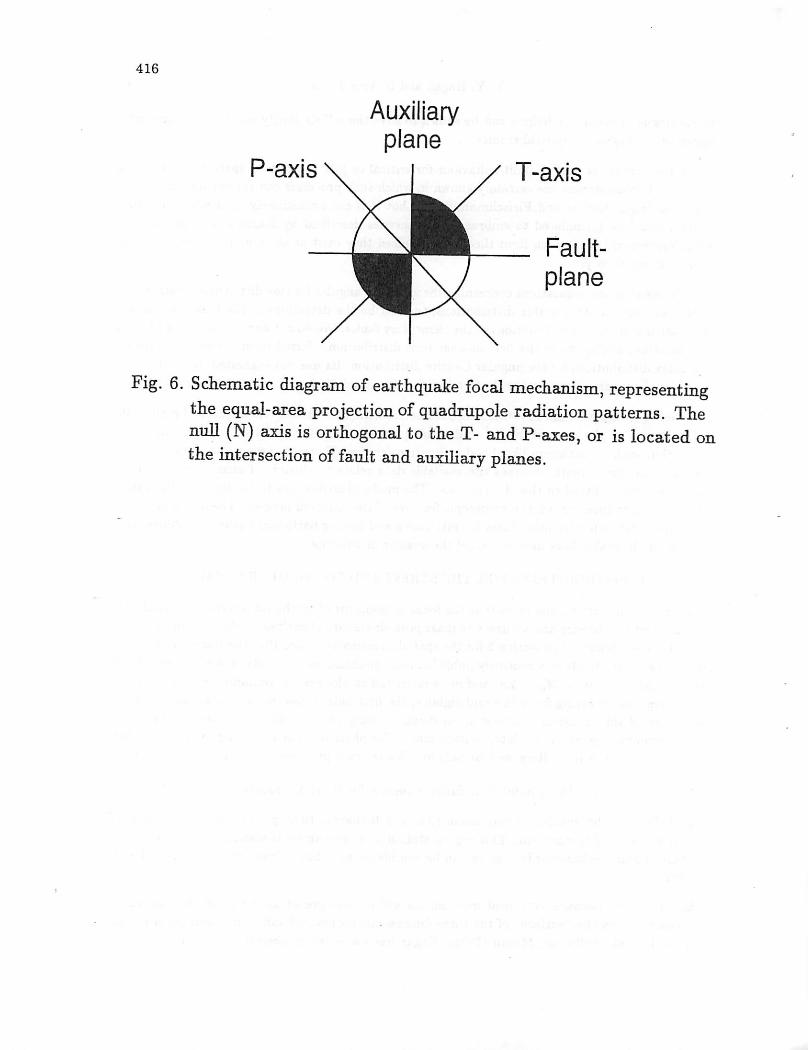
Note that in B(iii) the N. Pole is taken to be the orientation ofthe parent dislocation, and thatwe identify q with tt - q. An alternative point representation of B(ii) and B(iii) can be obtainedby treating the pair (orientation; direction ofmotion) as a point on the 3-dimensional surface S3of a 4-dimensional ball; then both aspects of the offspring distribution are controlled by a singleconcentration parameter r. The representation of such a 'focal mechanism' as a point on the 2-dimensional surface S2 of a 3-dimensional ball is familiar in seismology, where the focaJ mechanismisdepicted as a (2-dimensional picture of) a sphere divided into quadrants bya pole (point on S2)and a set of axes about that pole. Typical examples are shown in Fig 1(a); see also Fig 6 and thefurther discussion in section 4.1.

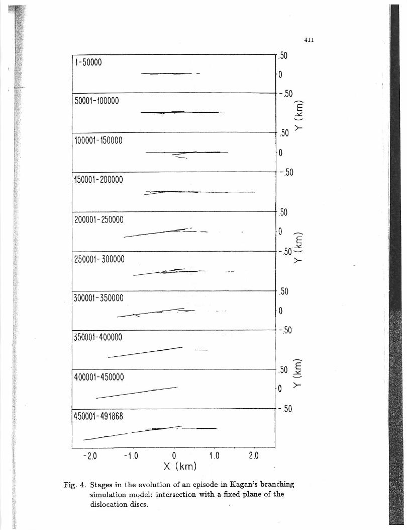
The simulationproceeds in two stages. In the first stage the branching family trees are startedfrom a number of initial ancestors, and the spatial coordinates (location of disc centre, orientation,and direction) are recorded. From the results of this stage, it is possible to obtain a visual pictureof the resulting "fractures" by plotting the intersection of the elementary discs with a fixed plane(see Fig. 4). It is partly from such pictures that the angular Cauchy distribution, rather thansome other angular analogue of the stable distributions, has been chosen. Experimentally theplots obtained reproduce visually, and in the case of some quantitative characteristics, such as thefractal dimensions, also quantitatively, the samesorts of features that are observed from geologicalmappings of fault traces.

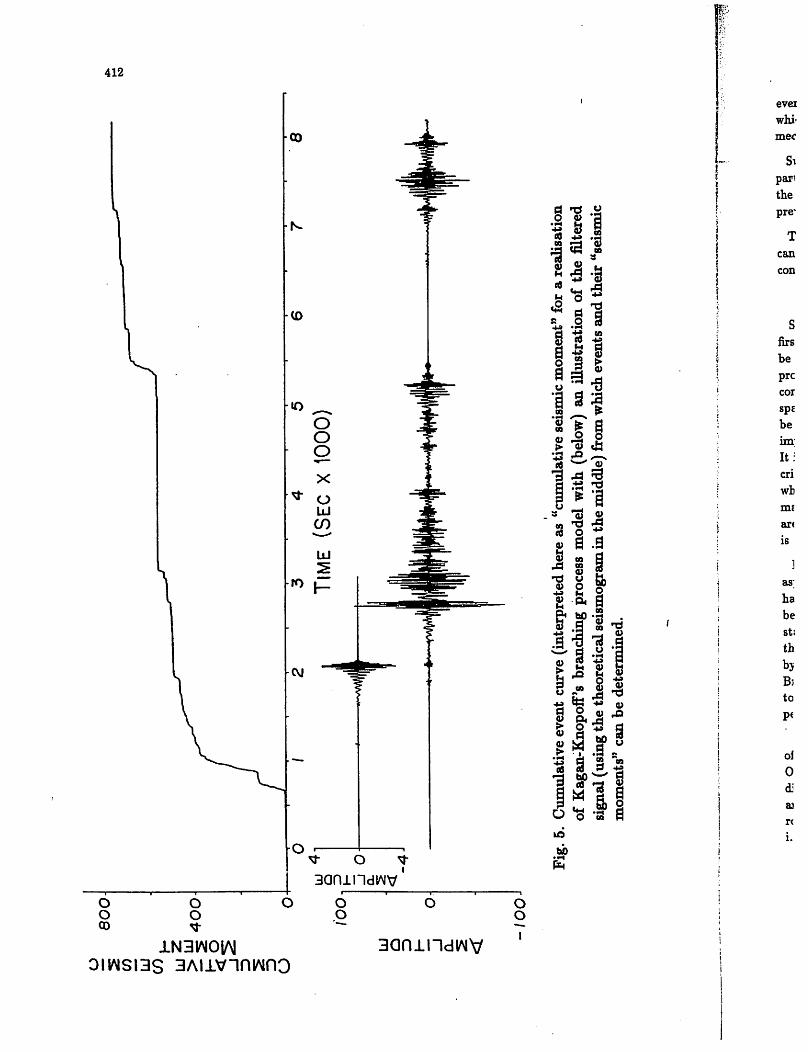
The second stage of simulationinvolves adding the time delays between the appearance of parentand offspring. With this information available, a cumulative plot of the number of elementaryevents against time can be obtained. (In seismologkal terms, eachelementary event is supposed tocontribute a fixed amount to a scalar moment release, so that cumulative plots can be interpretedasanalogues to the cumulative moment-release plots used in discussing realearthquake catalogues).The intense clustering of the near critical process results in this cumulative plot taking on a self-similar, step-function appearance. By convoluting the derivative of this cumulative function witha suitably shaped template, i.e. by examining a function of the form

X(t) = / H(t- u)dN(u),Jt-T

a time-series record can be obtained which may be compared with the trace of a seismograph, orits envelope, in the real situation. By applying similar criteria to those used in reality to identifyparticular events, Kagan is then able to produce from the time series record a list of simulated'events', each with its own 'magnitude' corresponding to the size of a local maximum in the plotof the time series (see Fig. 5). Moreover, by averaging the locations of the elementary dislocationsresulting in such an 'event', an approximate location for the 'hypocentre' of the event may bedetermined, representing roughly the centre of gravity (centroid) of the locations of the elementary

-50000

50001-100000

100001-150000

150001-200000

200001-250000

250001-300000

300001-350000

350001-400000

400001-450000

450001-491868

-2.0 -1.0 0 1.0

X (km)2.0

.50

-.50

411

.50

E

0

-.50

.50

0 .

-.50

.50

0

-.50

E

>-

.50 |

0 >-

-.50

Fig. 4. Stages in the evolution of an episode in Kagan's branchingsimulation model: intersection with a fixed plane of thedislocation discs.

-100

345

Time(Secx1000)

•it:/.•'i»,

Fig.5.Cumulativeeventcurve(interpretedhereas"cumulativeseismicmoment"forarealisationofKagan-Knopoff'sbranchingprocessmodelwith(below)anillustrationofthefilteredsignal(usingthetheoreticalseismograminthemiddle)fromwhicheventsandtheir"seismicmoments"canbedetermined.

8

f3EfrO2.•do*j*«o*tr"

t^sr«.»wEI"*-••....HmM*"»w>

on''3££**3H^*5

to

'i"$M

ieH?'

WrsIP

w3*;

¥•-&

* *!#'4»

&Nc

^

w

m


events contributing to the cluster. In this way a synthetic seismic catalogue can be produced, inwhich events are listed in time sequence and associated with a hypocentre, magnitude and focalmechanism.

Such a catalogue can then be treated in essentially the same way as the real catalogues. Inparticular, it is possible to compute the empirical the 2-, 3- and 4-point moment functions forthe synthetic catalogues, and see whether they exhibit features similar to those described in theprevious sections. According to K6, similar properties are in fact observed.

The question now arises as to how far the properties observed for the simulated cataloguescan be related to known properties of spatial branching processes. Some preliminary suggestionsconcerning this question are set out below.

3.2. Some Theoretical Considerations

Since many different limit relations exist for different types of branching processes, a desirablefirst step is to identify more precisely the contexts in which answers to the above question mightbe sought. The process lives in a space of 7 dimensions, so a natural first step is to consider itsprojections onto time and space axes only. Because of the assumed independence of the differentcomponents, this at first sight would seem to lead to a branching process in the lower dimensionalspace, with the other components simply ignored. However one important approximation has tobe made in so doing, which in the case of distributions with long tails could prove to be of crucialimportance. The caveat concerns the effect of simulating the process only within a bounded region.It is known, for example, that in spaces of dimension 2 or higher, stable regimes can exist even forcritical branching processes which would "explode" in a space of dimension 1. In such situationswhat happens at the boundaries is all-important, so that integrating out the unwanted variablesmay give a very misleading impression of the limit behaviour to be expected. The angular variablesare not so likely to cause trouble in this respect, since they take their values in a compact space; itis the space-time interaction which is likely to introduce problems.

Bearing this possible difficulty in mind, let us nevertheless consider first the purely temporalaspects of the process, ignoring spatial and angular coordinates of the points in the process. Wehave then a branching process along the time axis, in which the "gestation period" - the time lag

|| between the appearance ofan ancestor and its offspring - is distributed according toa non-negative||]'. stable distribution. In themodel thevalue oftheshape parameter isset at 1/2, but we may consider"!£ the moregeneralstable distribution with parameter a, 0 < a < 1. The choice a = 1/2 is motivatedjfe; by consideration of the first passage time to a fixed level (interpreted as a critical stress level) of aP Brownian motion. Since stress is a tensor, and moreover the ambient distributions are more likely|f to be stable than Gaussian, a first question is how robust is the first passage time distribution to|p perturbations ofthe underlying Gaussian model?HH Another justification of the choice a = 1/2 relates to the ability of the model with this choicefei of parameter to reproduce important features of the observed process, in particular the so-calledP Omori Law for the decay ofaftershock sequences. This lawasserts that the frequency ofaftershocksj| diminishes with time after the main shock at a rate proportional to (c+ i)~1-/l, where h is small*£ and often taken as zero. Within the model, the decay of an aftershock sequence will correspondfit?

If roughly to the decay of the expected number of offspringfrom an initial large number of ancestors,jl" i.e. it will be proportional to the first order intensity of the process startedfrom a single ancestor.

414 Statistical Models of Earthquake Occurrence

This obeys the renewal equation

h{t) =60(t) +m/ f{x)h(t - x)dx, (3.2)

(see, for example, Jagers, 1989; or Daley and Vere-Jones, 1988), thesolution of which has Laplacetransform

**w = [i-mrw]-1.

This solution has somerather special features when the inter-event distribution / has an infinitemean and is of stable form. If the mean number ofoffspring m < l,then h(x) decays asymptoticallyas a;"1-0, i.e at the same rate as f{x). If m = 1, then instead of approaching a constant (asit would if the mean time delay were finite) h(x) decays as jb~1+° . This suggests that if theprocess is imbedded into a process with immigration, then values of a close to zero, rather thana = 1/2, wouldproduce the better agreement with Omori's Law. However, in addition to the caveatmentioned above, there is also the fact that the events which are claimed to follow Omori's law,are not the infinitesimal elements of the original branching process, but groupings of such eventsselected because they stand out above some minimal background level. This selection procedurealone could produce substantial changes to the tail behaviour. It seems to us that further study,both of the model and of the simulation results, is needed to clarify the relationship to Omori'sLaw, and to further aspects the observed process such as the occurrence of "foreshocks" as well as"aftershocks" associated with a major event.

It may be worth pointing out that this projection of the K-K model onto the time axis is infact an example of the Hawkes' self-exciting model with an "infectivity function" (see Daley andVere-Jones, 1988,p. 367) proportional to the density of a stable distribution. Thus the K-K modelis really a fore-runner, in a space of higher dimension, of the space-time versions of the Hawkesprocess considered recently by authors such as Musmeci and Vere-Jones (1992).

Consider next the purely spatial aspects of the process. A simpler, 2-dimensional, version of themodel can be developed by replacing the dislocation loops by linear steps in the plane, each stephaving a centre (x,y) and direction q. Offspring are located with equal probability at either endof the step, with the offspring orientation following a 1-dimensional angular Cauchy distribution,with concentration parameter r, centred on the orientation of the parent step. The directions ofslip may be taken as always parallel to the step, with a high probabihty of following the sense ofthe parent step.

The result is a rather more easily visualized branching process of lines in the plane. Since eachstep can be represented as a point in R2 XS1, the process could also be represented as a branchingrandom walk along the surface of a 3-dimensional cylinder. If the step length and the time intervalwere rescaled suitably, it could no doubt be represented in the limit by an infinitely divisible processfor which the first two coordinates had a Brownian motion-like behaviour and the third was a stable

(Cauchy) process. What can be said about the fractal dimensionsof the trajectory of such a process,or its projection back on to the plane as a process of lines?

Let us now add in the time component, and consider the full process in space-time. Two principalquestions which need to be considered here are whether there exists a theoretical basis for theclustering properties which lead to the extraction of individual earthquake 'events', and whether


the catalogue of events so defined can be shown to have the self-similarity and moment propertiessuggested by Kagan's empirical studies.

Here the context is that of limit behaviour for critical or just sub-critical space-time branchingprocesses. Circumstances are certainly known in which such processes can exhibit limiting clusterproperties (e.g., Dawson and Fleischmann, 1988) but it is not immediately clear whether a limittheorem could be formulated to embrace the properties described by Kagan's simulations. Ourinitial impression is that such limit theorems, if indeed they exist at all, would require extensionsto the existing theory.

Finally we raise some questions concerning the use ofthe angular Cauchy distribution, rather thanangular variants of other stable distributions, to describe the deviations of the focal mechanisms(orientation and direction ofmotion) ofthe elementary faults. We do not know ifthere isa physicalinterpretation, analogous to the first passage time distribution referred to in connection with thetime-delay distribution, for the angular Cauchy distribution. Its use was suggested by comparisonsofthe visual appearance and othercharacteristics ofthe simulation model and the observed process.

This leads to the problem of estimating parameters within the model. As mentioned earlier, themodel belongs to the general family of Hawke's processes used successfully by many authors inconjunction with a maximum likelihood estimation scheme. However, because the model relatesonly to elementary events, whereas the available data relate to clusters of elementary events, itcannot be directly fitted to the observations. The model therefore has to be fitted on the extentto which it reproduces broader,macroscopic features of the observed process. The problemthen ishow to formulate effective procedures for estimating and testing particular parameter values, suchas those for the stable laws used to model the angular distributions.

4. DISTRIBUTIONS FOR THE STRESS AND FOCAL MECHANISMS.

It is only in the last decade or so that the focal mechanisms ofearthquakes have been publishedwithsufficient consistency and accuracy to makepossible statistical analyses of the focalmechanismssimilar to those described in section 2 for the spatial coordinates. Since 1977the Harvard catalogue(Dziewonski et al., 1994) now routinely publishes focal mechanisms for events on a world-wide basiswith moment magnitude Mw > 5.8, andmore restricted catalogues areavailable for smaller eventsin some regions. Starting from the mid-eighties, the first author has initiated a series of studiesmaking use of this material, opening up in doing so many new questions and avenues of study.A good account of progress to date, written mainly for physicists but reviewing many of the keystatisticalideas, is in K12. Here we look only at a few selected problems, basedmainlyon K9-K11.

4.1. The 2-point Correlation Function for Focal Mechanisms.

Fig. 6 displays the equal-area projection (Aki and Richards, 1980, p. 110) for an example ofan earthquake focal mechanism. This representation of a mechanism is standard in seismologicalliterature. Focal mechanisms in Fig. la can be considered as 3-dimensional rotations of the Fig. 6diagram.

The "distance" between two focal mechanisms will be interpreted as the rotation required tobring one point on the "surface" of the three-dimensional normalized sphere into coincidence withthe second point. Following Moran (1975), Kagan has suggested representing each such point in

416

P-axis

Auxiliaryplane

T-axis

Fault-

plane

Fig. 6. Schematic diagram of earthquake focal mechanism, representingthe equal-area projection of quadrupole radiation patterns. Thenull (N) axis is orthogonal to the T- and P-axes, or is located onthe intersection offault and auxiliary planes.

Statistical Models of Earthquake Occurrence 417

quaternion notation

q = go + qi * i + qi * j + q* * k,

where ijk are mutually orthogonal unit vectors satisfying i*i=j*j = k*k= —1 and i * j = k,j*k = i, k*i = j, and the scalars qi satisfy q\2 + q22 + qz2 + q±2 = 1. If we write go =cos(^/2), gi = sin(^/2) cos(0), q2 = sin(^/2) sin(0) cos(^), qz = sin(^/2) sin(0)sin(V'), then q canbe interpreted as a rotation from one event to the second through an angle <j> about an axis withspherical polar coordinates 0, ip.

Purely random (uniform) rotations correspond to selecting a direction at random on the 3-dimensional surface of 4-dimensional ball (Moran, 1975); in this case the rotation angle <f> hasa cumulative distribution of the form

^) = (l/7r)[^-cos(^)]. (4.1)

More generally we can generate an isotropic angular Cauchy distribution following the prescriptiongiven in section 2, in which case <f> has the marginal distribution

i^) = (l/x)[^-cos(^)]. (4.2)

where tan(^) = iirtan(^*). (In fact the same marginal will be obtained whenever the rotationangle is independent of the orientation of the axis)

To prepare the data for an analysis of the 2-point moment functions of the fault mechanisms,the key step is to develop an inversion procedure for determining the rotation q required to take amechanism qi into a mechanism q2. Details of the procedure are outlined in K9.

The situation is much complicated by the existence of symmetries, which introduce a form ofaliasing, or confounding, into the description of the distribution of ^. For example, the representation of a stress tensor in terms of quaternions is invariant under rotations of ic about any ofthe axes, corresponding to multiplication of the quaternion by any of the unit vectors i,j,k. Inrelation to fault mechanisms, such symmetries arise because in the routine determination of focalmechanism from the seismic records, it is not possible to distinguish between the fault plane andthe plane orthogonal to it and the direction of motion, nor to distinguish the sense of the faultmotion. The result is that there are in general four rotations that will take qi into one or otherof the equivalent representations of q2. From these the one with the smallest value of <j> may beselected. This has the effect of folding back some of the original ^-distribution onto itself. Inparticular it turns out that there is always at least one rotation with a 0 of 2x/3 or less, so themodified distribution of (f> is restricted to the range (0,2ir/3). Again we refer to K9 for details.

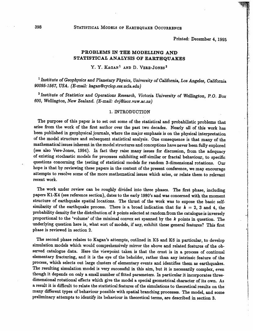
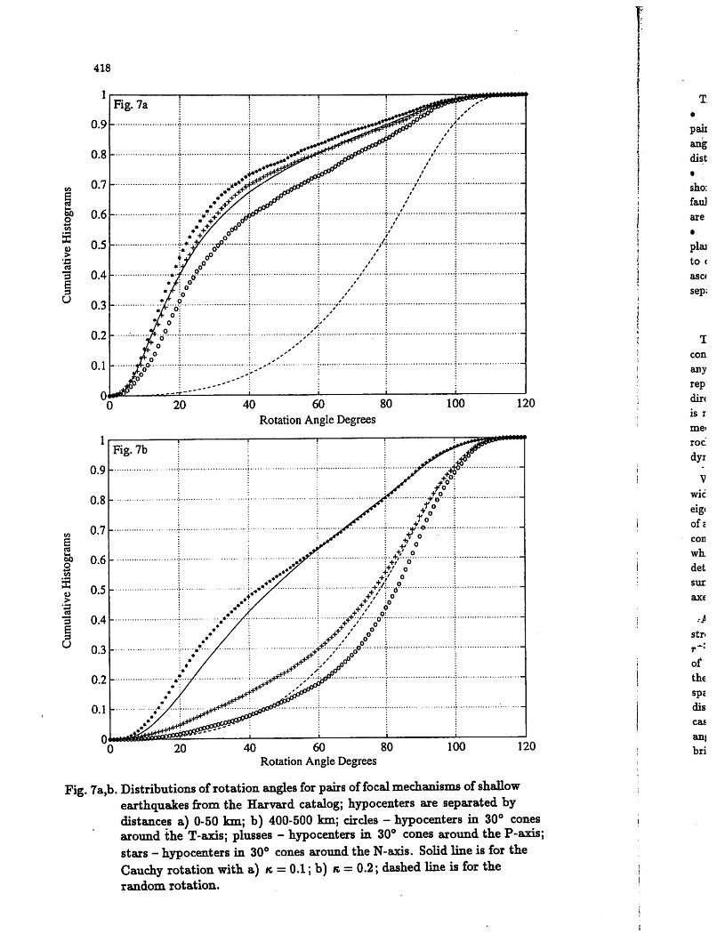
Since it is impossible to measure the total stress at seismogenic depths where earthquakes originate, Kagan (K9) measured the angles of focal mechanism rotation for any pair of earthquakes inthe Harvard catalog. If the stress is a smooth spatial function, the angles of neighbouring eventswould be small, thus these angles indicate the degree of the stress irregularity. In Fig. 7 we show anexample of the angle distribution for earthquakes separated by various distances and situated alonga fault plane (around the JV-axis, see Fig. 6) or outside the plane (around the T- and P-axes).Two theoretical curves show the rotational Cauchy and the uniform random rotation (see morein K9). For small distances between the earthquake centroids the angle distributions are approximated by the Cauchy curve, whereas for large distances only the events aligned along a fault planeare Cauchy distributed; for other earthquakes the rotation angle is uniformly random.

ECO

Q

3

a3

u

418

20

20

40 60 80

Rotation Angle Degrees

40 60 80

Rotation Angle Degrees

100

100

120

120

Fig. 7a,b. Distributions ofrotation angles for pairs offocal mechanisms ofshallowearthquakes from the Harvard catalog; hypocenters are separated bydistances a) 0-50 km; b) 400-500 km; circles - hypocenters in 30° conesaround the T-axis; plusses - hypocenters in 30° cones around the P-axis;stars - hypocenters in 30° cones around the N-axis. Solid line is for theCauchy rotation with a) k, = 0.1; b) n= 0.2; dashed line is for therandom rotation.

paii

ang

dist

•

sho:

fad

are

•

plaito (

asc<

sep;

T

con

any

rep

dirt

is r

mei

roc

dyi

V

wic

eigiofE

con

wh.

det

sur

ax(

str<

r~:

of

th€

Spc

dis

cas

ani

bri

Fm

farA:

s

fc

$i


The empirical results are set out in K9in more detail, andmaybe briefly summarised as follows.• (i) For most distances, angular separations and time intervals from the initial event in thepair, the distribution of the rotation angle <f> appears to be reasonably well approximated by anangular Cauchy distribution ofthe general form (4.2), but not well approximated by other angulardistributions such as the Fisher distribution.

• (ii) The concentration parameter k, on the other hand, varies appreciably with these factors. Atshort distance and time intervals, the distributionis mosthighly concentratedalong the directionoffault motion, but becomes less concentrated as the distances, timeintervals and angular separationsare increased.

• (iii) the distribution of the parameters 0and if;, representing the shift inorientation of the faultplane, does not appear to be uniformly distributed over the unit sphere; it shows some tendencyto concentrate on smaller values, but the high dimensionality of the study makes it difficult toascertain any clear pattern in the variation ofthe distribution as a function ofdistance, angularseparation or time.

4.2. Distributions of Stress Fields.

The branching model described in section 3 is purely kinematic; forces do not appear. In acontinuous medium, forces are traditionally described in terms ofa stress field, with the stress atany point represented by a 3 X3 stress tensor, or matrix. Each element <r(z, j) of the matrixrepresents the component of force acting indirection j on an element ofsurface perpendicular todirection i, where i,j,k correspond to three orthogonal reference directions in the medium. Itis not entirely clear that such a description is appropriate for a highly heterogeneous, fracturedmedium such as the earth's crust, but nevertheless stress calculations play a highly useful role inrock mechanics and in seismology, and they seem the natural starting point in trying to develop adynamic model.

We need to recall a few further terms and properties of the stress tensor. The matrix underwide conditions is symmetric, and therefore has three real eigenvalues associated with three real

!| eigenvectors. The latter determine the axes of principal stress. The forces acting across an element| of area orthogonal to one of these axes are purely normal to the surface. For all other directions theyI contain botha normal and a tangential or shear component. The latterisa maximumfbr directionsHI which bisect the angles between the principal axes. The coefficients in the characteristic polynomialI det(A *I- S) of the stress matrix £ form the three stress invariants, the first representing just the

sum of the principal stresses. The stress invariants are independent of the choice of the referenceaxes, and determine the size and shape ofthe stress ellipsoid or other conic.

Any discontinuity, such as a dislocation, in the medium will cause a local perturbation to the| stress field. It will be important in the sequel that the effects of such perturbations decay asI r-3, where r is the distance from the perturbation, at least for r outside the immediate vicinityj§ of the perturbation. Zolotarev and Strunin (1971) (see also Zolotarev, 1986) have shown that if|| the perturbations are distributed uniformly at random (i.e., following aPoisson process) throughI space, the components of the stress tensor at an arbitrary point of the space follow a CauchyI distribution. In K8 and K9, using partly analytic and partly simulation methods, some specialI cases are examined in detail, and used to justify the use of Cauchy distributions, both spatial and|| angular, in the branching model. As the assumptions underlying this argument are important, we!f briefly reproduce it below.

I*


Suppose thesources are located at points xk{ukt 0k, $k) >where to take advantage ofthe symmetrywe have taken asigned distance u(-oo<u<oo), with restriction ofthe latitude 0 (0 < 0 < ir/2),in place or the usual r, 0, rp of spherical polar coordinates. Now consider the net contributionfrom all sources to a given component ofthestress tensor at the origin. This takes the form ofthesum

oo f/2 2-tc

S=Y,f(0k,1>k)/\(uk)\3= j //sign(u)/(^,^)/|(«)|3^K^^),-oo 0 0

where N denotes counting measure and f(0ki<f>k) describes the resolution of a unit vector, directedtowards Xk, along the chosen direction of the stress field. We have then to find the characteristicfunction of the distributionof 5, c(t) = E[exp(itS)]. Examination of this expectationshows that itis nothing other than the characteristic functional of the point process N, evaluatedfor the specialchoice of carrier function £exp{it/()/|(ti)|3}. The ch. fl. of the homogeneous Poisson process $(£)is given by

§(£) =exp{J[exp(mx)) - l]dx}.Substituting for £ and changing variable from u to y = f()/u3 we can rewrite the characteristicfunction c(i) in the form

oo

c(t) =J{[exrftty) - l]/\y\(l+a)}dy j'{/(*, *)ad0ty}, (4.3)—oo

where a = 1 in the present case. The y-integral is recognisable as the characteristic function ofthe symmetric stable distribution with parameter a, i.e., the Cauchy distribution in the presentinstance. Exactly similar argument can be used to derive the Holtzmark distribution (a = 3/2) forthe gravitational field due to Poisson distributed stars. It should be noted that both these fields havelong-tailed distributions, distinguishing them from examples such as fractional Brownian motionand their relatives, in which the field variables have short-tailed distributions.

There are a number of questions and comments which arise in relation to the above derivation.• (i) The argument as given applies to a single scalar component of the stress field. It wouldseem possible in principle to extend the argument to the joint distribution of the stress components. Is this indeed possible, and does it lead to the Cauchy angular distribution for the directionof principal stress?• (ii) Is the conclusion affected by introducing distributions for the sizes and orientations of therandom perturbations?• (iii) Can the argument be extended to situations where the sources have a self-similar distribution, resulting in a change of index to the derived stable distribution.

The last of these questions is of particular interest. Kagan has several times suggested that thismay be the case, (see, e.g., comments in K10-K12), and has found empirically that distributionswhich appear to be of stable type with index different from one arise in simulations of self-similarpatterns, and for the data from the Harvard catalogue, using standard formulae for the stress fieldproduced at distance for the double-couple model of earthquake fault mechanism. Justifying thisresult analytically, however, runs into the same sort of difficulty as that described in section 2c:exactly what are we to assume for the distribution of sources? The argument leading to (4.3)


depends rather crucially on the Poisson character of the underlying point process. This would seemto restrict us to the processes discussed in section 2.2c (Poisson with singular parameter measure),and hence to the difficulties noted in that section.

A more practical question related to this discussion is• (iv) Find robust methods of inference for the index of a symmetric stable distribution. The robustness is needed because the empirical distribution will usually be contaminated by measurementerrors or boundary effects at the ends of the distribution, so that only some part of the distributionis properly available for inference.

To conclude this section we note the work in Kll and K12 in which similar ideas are used to

compute the increments to the local stress field caused by recent earthquakes in the Californiaregion. Clearly the results are very tentative, and in themselves take no account of any pre-existingstress field, or increases due to plate motion. Nevertheless one can begin to see from the patternsproduced how the stress regime over a region may evolve, and in its turn serve to initiate futureearthquakes, thus exhibiting on a large and complex scale the same branching, self-organisingbehaviour studied on a small scale and in idealised fashion with the simulation model.

5. SUMMARY AND FURTHER REMARKS.

We summarize below the main points to arise from the preceding discussion.

(i) There seems to be some general difficulty in knowing how best to approach models for point',». process data that exhibit selfsimilarity andfractal behaviour. For example, we do not know if any' legitimate models exist for processes which exhibit the 1/V dependence for the 4-point moment

function claimed by Kagan for earthquake catalogues. An underlying question is whether thestandardpoint process framework is adequate to discuss problems of this kind, and if not, how it

ir should be extended.t

| (ii) There are a number of related questions on which we lack current information. How far!', has the idea of "Palm stationarity" been explored? What can be said about processes exhibiting

"intermittent" self-similarity? What are the most appropriate extensions offractal and multifractal' dimension to point process models? References and suggestions would be welcome.

\ (iii) The analytical properties ofthe K-K branching model remain almost completely unexplored.Two immediate questions which arise concern thefractal dimension ofrealizations oftheprocess and

|- the existence ofcluster limit theorems which might provide a theoretical underpinning to Kagan'sL empirical results on the self-similarity and other properties of the derived process of simulated"/ "earthquakes".

; (iv) Many statistical and modelling questions arise in the representation offocal mechanismsI and stress tensors as points on a three-dimensional space. Kagan's rotational Cauchy distributions% appear toplay a key role here, but again they lack a proper theoretical underpinning. Can they be£ derived from an extension of Zolotarev's derivation ofthe ordinary Cauchy distribution for a scalar*' component ofthe stress field? Do further extensions ofZolotarev's theory exist for the stress fieldi in a non-homogeneous but still setf-similar field ofrandomly distributed defects?

(v) Anumber ofmore immediate statistical questions arise out ofKagan's work, which space hasprecluded us from treating in detail, but which we mention here by way of conclusion, (a) What


are efficient estimation and testing procedures for the 3-D rotational Cauchy distributions? (b)Given that branching process models tend to suggest distributions of the form

Prob(-X" > x) = x"^exp[-7(x - 1)],

what are the best ways oftesting for constancy of the parameters in thespatial domain? (c) Whatare robust ways oftesting the value of the parameter a ina symmetric stable distribution (robusthere meaning that data from the centre and the extremes ofthe distribution may be suspect)?

Acknowledgments.

This research was supported in part by Grant VIC406 of New Zealand Foundation for Research,Science & Technology. We are grateful for useful discussions with R. B. Davies. PubUcation 4290,Institute of Geophysics and Planetary Physics, University of California, Los Angeles.


References

Aki, K., and P. Richards, 1980. Quantitative Seismology, W. H. Freeman, San Francisco, 2 Vols,557 and 373 pp.

Chong, F. S., 1983. Time-space-magnitude interdependence ofupper crustal earthquakes in themain seismic region of New Zealand, N. Z. J. Geol. Geophys., 26, 7-24.

Cutler, CD., 1991. Some results on the behaviour and estimation of the fractal dimensions ofdistributions on attractors, J. Statist. Phys., 62, 651-708.

Daley, D. J., and D. Vere-Jones, 1988. An Introduction to the Theory of Point Processes, NewYork, Springer-Verlag, pp. 702.

Dawson, D. A., and K. Fleischmann, 1988. Strong clumping of critical branching models insubcritical dimensions, Stochastic Process. Appi, 30, 193-208.

Dziewonski, A. M., G. Ekstrom, and M. P. Salganik, 1994. Centroid-moment tensor solutions forJanuary-March, 1994, Phys. Earth Planet. Inter., 86, 253-261.

Geilikhman, M. B., T.V. Golubeva, and V. F.Pisarenko, 1990. Multifractalpatterns ofseismicity,Earth and Plan. Sci. Letters, 99, 127-132.

Hawkes, A. G., and L. Adamopoulos, 1973. Cluster models for earthquakes - Regional comparisons, Bull. Int. Statist. Inst, 45(3), 454-461.

Hawkes, A. G., and D. Oakes, 1974. A cluster representation of a self-exiting process, /. Appl.Prob., 17, 493-503.

Jagers, P., 1989. General branching processes as a random field, Stochastic Process. Appi, 32,183-212.

Kagan, Y. Y., 1973. Statistical methods in the study of the seismic process, Bull Int. Statist.Inst, 45(3), 437-453.

Kagan, Y. Y., 1981a. Spatial distribution of earthquakes: the three-point moment function,Geophys. J. Roy. astr. Soc, 67, 697-717 (K2).

Kagan, Y. Y., 1981b. Spatial distribution of earthquakes: the four-point moment function,Geophys. J. Roy. astr. Soc, 67, 719-733 (K3).

Kagan, Y. Y., 1982. Stochastic model of earthquake fault geometry, Geophys. J. R. astr. Soc,71, 659-691, (K6).

Kagan, Y. Y., 1990. Random stress and earthquake statistics: spatial dependence, Geophys. J.Int., 102, 573-583, (K8).

Kagan, Y. Y., 1991. Fractal dimension of brittle fracture, J. Nonlinear Sci., 1, 1-16, (K4).

Kagan, Y. Y., 1992. Correlations of earthquake focal mechanisms, Geophys. J. Int., 110, 305-320,(K9).

Kagan, Y. Y., 1994a. Incremental stress and earthquakes, Geophys. J. Int., 117, 345-364, (K10).


Kagan, Y. Y., 1994b. Distribution of incremental static stress caused by earthquakes, NonlinearProcesses in Geophysics, 1,172-181, (Kll).

Kagan, Y. Y., 1994c. Observational evidence for earthquakes as a nonlinear dynamic process,Physica D, 77,160-192, (K12).

Kagan, Y. Y. and L. Knopoff, 1980. Spatial distribution ofearthquakes: the two-point correlationfunction, Geophys. J. Roy. astr. Soc, 62, 303-320, (Kl).

Kagan, Y. Y. and L. Knopoff, 1981. Stochastic synthesis of earthquake catalogs, /. Geophys.Res., 86, 2853-2862, (K5).

Kagan, Y. Y. and L. Knopoff, 1987. Random stress and earthquake statistics: time dependence,Geophys. J. R. astr. Soc, 88, 723-731, (K7).

Mandelbrot, B. B., 1975. Sur un modele decomposable d'Universe hierarchise: deduction descorrelations galactiques surla sphere celeste. C. R. Acad. Sc. Paris, 280, Ser. A, 1551-1554.

Mandelbrot, B.B., 1983. The Fractal Geometry ofNature, W. H. Freeman, San Francisco, Calif.,2nd edition, pp. 468.

Moran, P. A. P., 1975. Quaternions, Haar measure and estimation ofpaleomagnetic rotation, in:Perspectives in Probability and Statistics, ed. J. Gani, Acad. Press, 295-301.

Musmeci, F., and D. Vere-Jones, 1992. A space-time clustering model for historical earthquakes,Ann. Inst. Statist. Math., 44, 1-11.

Ogata" Y., and K. Katsura, 1991. Maximum likelihood estimates of the fractal dimension forrandom point patterns, Biometrika, 78, 463-474.

Otsuka, M., 1972. A chain-reaction-type source model as a tool to interpret the magnitude-frequency relation of earthquakes, /. Phys. Earth, 20, 35-45.

Ripley, B. D., 1977. Modelling spatial patterns, /. Roy. Stat Soc, B39, 172-212.

Saito, M., M. Kikuchi, and M. Kudo, 1973. Analytical solution of "Go-game model of earthquakes", Zisin, 26(2), 19-25.

Stoyan, D., 1994. Caution with fractal point patterns. Statistics, 25, 267-270.

Stoyan, D., W. S. Kendall, and J. Mecke, 1987. Stochastic Geometry and its Applications, NewYork, Wiley, 345 pp.

Stoyan, D., and H. Stoyan, 1994. Fractals, Random Shapes, and Point Fields: Methods of Geometrical Statistics, New York, Wiley, 389 pp.

Vere-Jones, D., 1976. A branching model for crack propagation, Pure Appi. Geophys., 114,711-725.

Vere-Jones, D., 1978. Space time correlations for microearthquakes - a pilot study, Adv. Appi.Prob. (Suppl. - Spatial Patterns and Processes), 10, 73-87.

Vere-Jones, D., 1994. Statistical models for earthquake occurrence: clusters, cycles and characteristic earthquakes, in Proc. First US/Japan Conf. on Frontiers of Statistical Modeling: AnInformational Approach, ed. by H. Bozdogan, pp. 105-136, Kluwer Publ., Netherlands.

&

1iff.;

ll:'.'"';•

r:

I


Vere-Jones, D., and D. Harte, 1995. Dimension estimates of earthquake epicentres and hypocentres, (VUW preprint: inpreparation).

Vere-Jones, D., R. B. Davies, D. Harte, T. Mikosch and Q. Wang, 1995. Problems and samplesin the estimation offractal dimension from meteorological and earthquake data, Ed. T. SubbaRao, Proc. Int. Con/, on Application of Time Series in Physics, Astronomy and Meteorology,Padua, (to appear).

Zolotarev V. M., and B. M. Strunin, 1971. Internal-stress distribution for arandom distributionof point defects, Soviet Phys. Solid State, 13, 481-482 (English translation).

Zolotarev, V. M., 1986. One-Dimensional Stable Distributions, Amer. Math. Soc, Providence,R.I., pp. 284.

Documents

Volume I: Applied Probability