Embed Size (px)
Citation preview

An Introduction to AppliedProbability Models
Peter S. FaderUniversity of Pennsylvania
www.petefader.com
Bruce G. S. HardieLondon Business Schoolwww.brucehardie.com
Workshop on Customer-Base Analysis
Johann Wolfgang Goethe-Universität, Frankfurt
March 8–9, 2006
©2006 Peter S. Fader and Bruce G. S. Hardie
1
Problem 1:Projecting Customer Retention Rates
(Modeling Discrete-Time Duration Data)
2

Background
One of the most important problems facing
marketing managers today is the issue of customer
retention. It is vitally important for firms to be able to
anticipate the number of customers who will remain
active for 1,2, . . . , T periods (e.g., years or months) after
they are first acquired by the firm.
The following dataset is taken from a popular book
on data mining (Berry and Linoff, Data Mining
Techniques, Wiley 2004). It documents the “survival”
pattern over a seven-year period for a sample of
customer who were all “acquired” in the same period.
3
# Customers Surviving At Least 0–7 Years
Year # Customers % Alive
0 1000 100.0%
1 869 86.9%
2 743 74.3%
3 653 65.3%
4 593 59.3%
5 551 55.1%
6 517 51.7%
7 491 49.1%
Of the 1000 initial customers, 869 renew their contracts at
the end of the first year. At the end of the second year, 743
of these 869 customers renew their contracts.
4
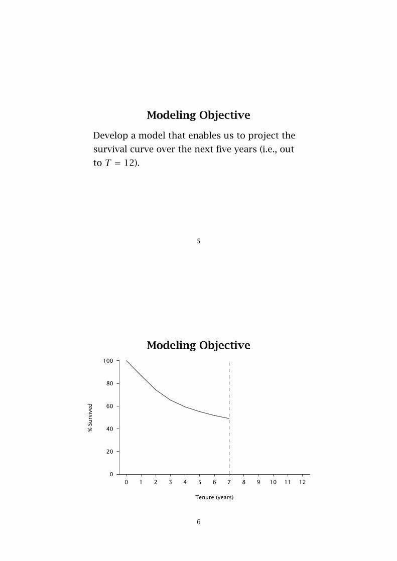
Modeling Objective
Develop a model that enables us to project the
survival curve over the next five years (i.e., out
to T = 12).
5
Modeling Objective
0 1 2 3 4 5 6 7 8 9 10 11 12
Tenure (years)
0
20
40
60
80
100
%Su
rviv
ed
...............................................................................................................................................................................................................................................................................................................................................................................................
6
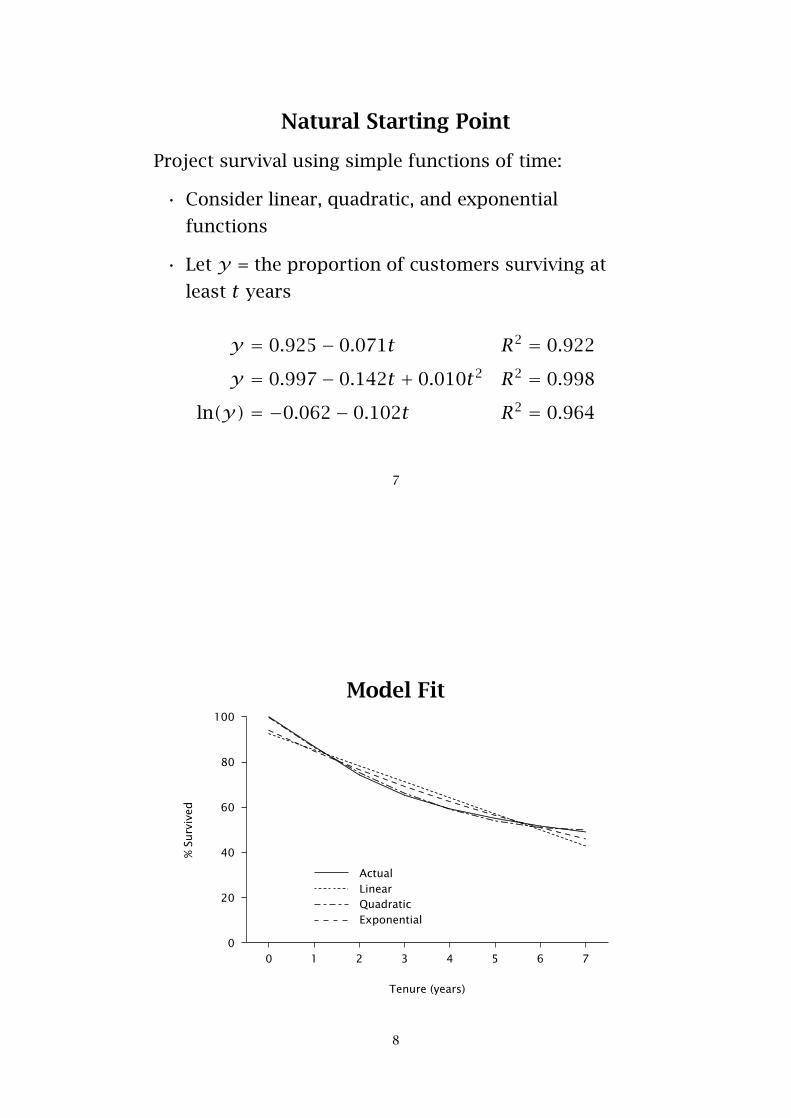
Natural Starting Point
Project survival using simple functions of time:
• Consider linear, quadratic, and exponential
functions
• Let y = the proportion of customers surviving at
least t years
y = 0.925− 0.071t R2 = 0.922
y = 0.997− 0.142t + 0.010t2 R2 = 0.998
ln(y) = −0.062− 0.102t R2 = 0.964
7
Model Fit
0 1 2 3 4 5 6 7
Tenure (years)
0
20
40
60
80
100
%Su
rviv
ed
...............................................................................................................................................................................................................................................................................................................................................................................................................................................................................................................................................................
Actual
............................................................................................................................................................................................................................................................................................
Linear
.....................................................................................................................................................................................................................................................................................................................................................
Quadratic
........ ........ ........ ........ ........ ........ ........ ........ ........ ........ ........ ........ ........ ........ ........ ........ ........ ........ ........ ........ ........ ........ ........ ........ ........ ........ ........ ........ ........ ........ ........ ........ ........ ........ ........ ...
Exponential
8

Survival Curve Projections
0 1 2 3 4 5 6 7 8 9 10 11 12
Tenure (years)
0
20
40
60
80
100
%Su
rviv
ed
..........................................................................................................................................................................................................................................................................................................................................................................................................................................................................................................................................................................................................................................
Actual
................................................................................................................................................................................................................................................................................................................................................
Linear
............................................................................................................................................................................................................................................................................................................
..............................
.......................
..................
..............................
Quadratic
................................ ........ ........ ........ ........ ........ ........ ........ ........ ........ ........ ........ ........ ........ ........ ........ ........ ........ ........ ........ ........ ........ ........ ........ ........ ........ ........ ........ ........ ........ ........ ........ ........ ........ ........ ........ ........ .....
Exponential
9
Developing a Better Model (I)
Consider the following story of customer behavior:
i. At the end of each period, an individual renews his
contract with (constant and unobserved) probability
1− θ.
ii. All customers have the same “churn probability” θ.
10
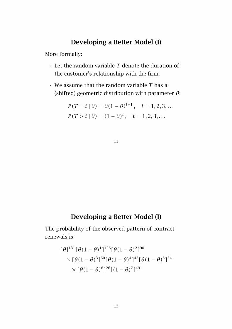
Developing a Better Model (I)
More formally:
• Let the random variable T denote the duration of
the customer’s relationship with the firm.
• We assume that the random variable T has a
(shifted) geometric distribution with parameter θ:
P(T = t |θ) = θ(1− θ)t−1 , t = 1,2,3, . . .
P(T > t |θ) = (1− θ)t , t = 1,2,3, . . .
11
Developing a Better Model (I)
The probability of the observed pattern of contract
renewals is:
[θ]131[θ(1− θ)1]126[θ(1− θ)2]90
× [θ(1− θ)3]60[θ(1− θ)4]42[θ(1− θ)5]34
× [θ(1− θ)6]26[(1− θ)7]491
12
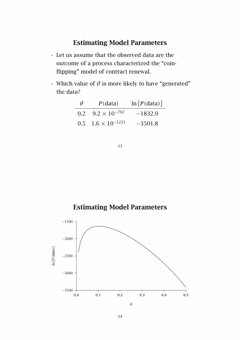
Estimating Model Parameters
• Let us assume that the observed data are the
outcome of a process characterized the “coin-
flipping” model of contract renewal.
• Which value of θ is more likely to have “generated”
the data?
θ P(data) ln[P(data)
]0.2 9.2 × 10−797 −1832.9
0.5 1.6 × 10−1221 −3501.8
13
Estimating Model Parameters
0.0 0.1 0.2 0.3 0.4 0.5
θ
−3500
−3000
−2500
−2000
−1500
ln[ P(d
ata)]
.........................................................................................................................................................
................................................................................................................................................................................................................................................................................................................................................................................................................................................................................................................................................................................................................................................
14
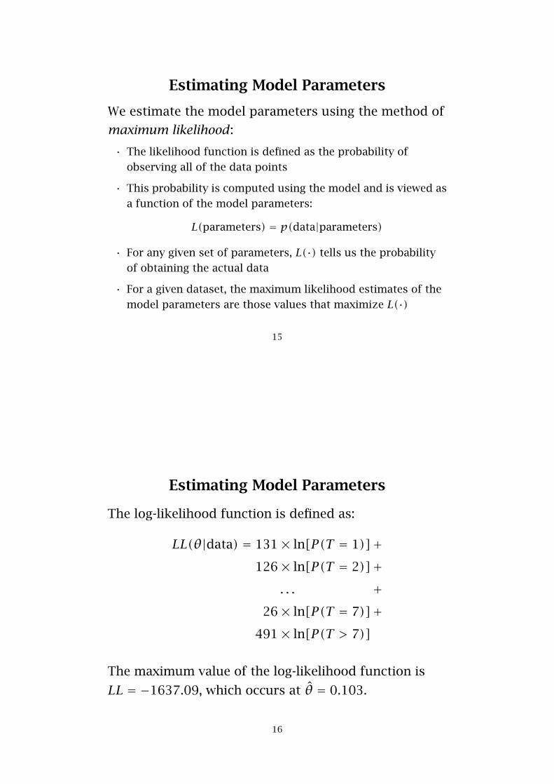
Estimating Model Parameters
We estimate the model parameters using the method of
maximum likelihood :
• The likelihood function is defined as the probability of
observing all of the data points
• This probability is computed using the model and is viewed as
a function of the model parameters:
L(parameters) = p(data|parameters)
• For any given set of parameters, L(·) tells us the probability
of obtaining the actual data
• For a given dataset, the maximum likelihood estimates of the
model parameters are those values that maximize L(·)
15
Estimating Model Parameters
The log-likelihood function is defined as:
LL(θ|data) = 131× ln[P(T = 1)]+126× ln[P(T = 2)]+
. . . +26× ln[P(T = 7)]+
491× ln[P(T > 7)]
The maximum value of the log-likelihood function is
LL = −1637.09, which occurs at θ̂ = 0.103.
16
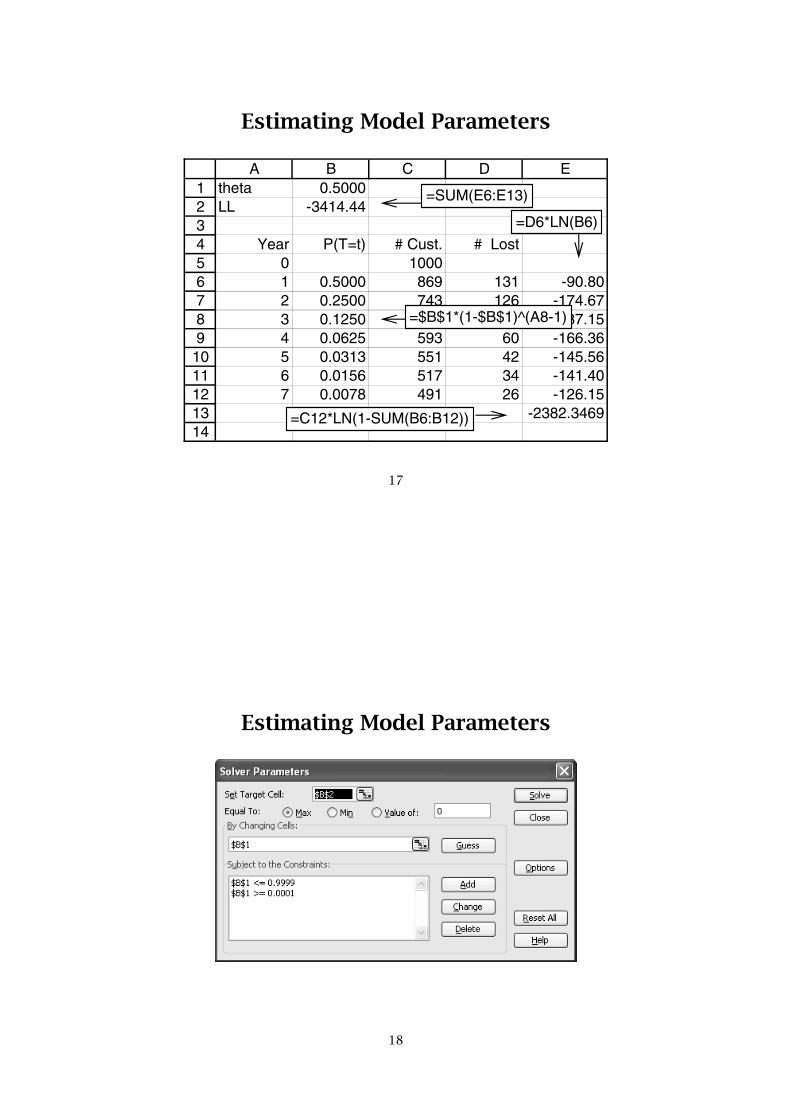
Estimating Model Parameters
1234567891011121314
A B C D Etheta 0.5000LL -3414.44
Year P(T=t) # Cust. # Lost0 10001 0.5000 869 131 -90.802 0.2500 743 126 -174.673 0.1250 653 90 -187.154 0.0625 593 60 -166.365 0.0313 551 42 -145.566 0.0156 517 34 -141.407 0.0078 491 26 -126.15
-2382.3469
=SUM(E6:E13)
=D6*LN(B6)
=C12*LN(1-SUM(B6:B12))
=$B$1*(1-$B$1)^(A8-1)
17
Estimating Model Parameters
18

Survival Curve Projection
0 1 2 3 4 5 6 7 8 9 10 11 12
Tenure (years)
0
20
40
60
80
100
%Su
rviv
ed
..........................................................................................................................................................................................................................................................................................................................................................................................................................................................................................................................................................................................................................................
Actual
........................................ ........ ........ ........ ........ ........ ........ ........ ........ ........ ........ ........ ........ ........ ........ ........ ........ ........ ........ ........ ........ ........ ........ ........ ........ ........ ........ ........ ........ ........ ........ ........ ........ ........ ........ ........ ........
Geometric
19
What’s wrong with this story of customer
contract-renewal behavior?
20

Developing a Better Model (II)
Consider the following story of customer behavior:
i. At the end of each period, an individual renews his
contract with (constant and unobserved) probability
1− θ.
ii. “Churn probabilities” vary across customers.
21
Developing a Better Model (II)
More formally:
i. The duration of an individual customer’s
relationship with the firm is characterized by the
(shifted) geometric distribution with parameter θ.
ii. Heterogeneity in θ is captured by a beta distribution
with pdf
f(θ |α,β) = θα−1(1− θ)β−1
B(α,β).
22

The Beta Function
• The beta function B(α,β) is defined by the integral
B(α,β) =∫ 1
0tα−1(1− t)β−1dt, α > 0, β > 0 ,
and can be expressed in terms of gamma functions:
B(α,β) = Γ(α)Γ(β)Γ(α+ β) .
• The gamma function Γ(z) is defined by the integral
Γ(z) =∫∞
0tz−1e−tdt, z > 0 ,
and has the recursive property Γ(z + 1) = zΓ(z).
23
The Beta Distribution
f(θ |α,β) = θα−1(1− θ)β−1
B(α,β), 0 < θ < 1 .
• The mean of the beta distribution is
E(θ) = αα+ β
• The beta distribution is a flexible distribution … and
is mathematically convenient
24
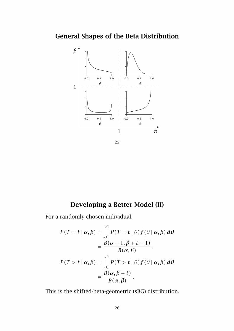
General Shapes of the Beta Distribution
�
�
α
β
1
1
0.0 0.5 1.0
................................................................................................................................................................................................................................................................................................................
θ
0.0 0.5 1.0
........................................................................................................................................................................................................................................................
θ
0.0 0.5 1.0
...........................................................................................
........................................................
.....................................................................................................
θ
0.0 0.5 1.0
........
.........
........
.........
.........
........
.........
..................................................................................................................................................................................................................................................................
θ
25
Developing a Better Model (II)
For a randomly-chosen individual,
P(T = t |α,β) =∫ 1
0P(T = t |θ)f(θ |α,β)dθ
= B(α+ 1, β+ t − 1)B(α,β)
.
P(T > t |α,β) =∫ 1
0P(T > t |θ)f(θ |α,β)dθ
= B(α,β+ t)B(α,β)
.
This is the shifted-beta-geometric (sBG) distribution.
26
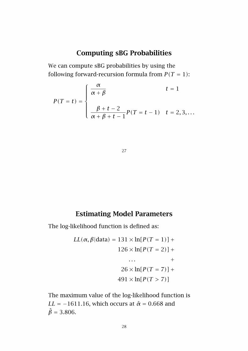
Computing sBG Probabilities
We can compute sBG probabilities by using the
following forward-recursion formula from P(T = 1):
P(T = t) =
⎧⎪⎪⎪⎪⎪⎨⎪⎪⎪⎪⎪⎩
αα+ β t = 1
β+ t − 2α+ β+ t − 1
P(T = t − 1) t = 2,3, . . .
27
Estimating Model Parameters
The log-likelihood function is defined as:
LL(α,β|data) = 131× ln[P(T = 1)]+126× ln[P(T = 2)]+
. . . +26× ln[P(T = 7)]+
491× ln[P(T > 7)]
The maximum value of the log-likelihood function is
LL = −1611.16, which occurs at α̂ = 0.668 and
β̂ = 3.806.
28
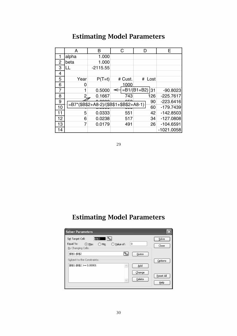
Estimating Model Parameters
1234567891011121314
A B C D Ealpha 1.000beta 1.000LL -2115.55
Year P(T=t) # Cust. # Lost0 10001 0.5000 869 131 -90.80232 0.1667 743 126 -225.76173 0.0833 653 90 -223.64164 0.0500 593 60 -179.74395 0.0333 551 42 -142.85036 0.0238 517 34 -127.08087 0.0179 491 26 -104.6591
-1021.0058
=B1/(B1+B2)
=B7*($B$2+A8-2)/($B$1+$B$2+A8-1)
29
Estimating Model Parameters
30
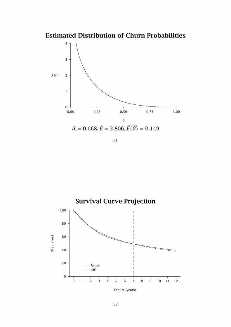
Estimated Distribution of Churn Probabilities
0.00 0.25 0.50 0.75 1.00
θ
0
1
2
3
4
f(θ)
...............................................................................................................................................................................................................................................................................................................................................................................................................................................................................................................................................................................................................................................................................................................................................................
α̂ = 0.668, β̂ = 3.806,E(θ) = 0.149
31
Survival Curve Projection
0 1 2 3 4 5 6 7 8 9 10 11 12
Tenure (years)
0
20
40
60
80
100
%Su
rviv
ed
..........................................................................................................................................................................................................................................................................................................................................................................................................................................................................................................................................................................................................................................
Actual
........................................................................ ........ ........ ........ ........ ........ ........ ........ ........ ........ ........ ........ ........ ........ ........ ........ ........ ........ ........ ........ ........ ........ ........ ........ ........ ........ ........ ........ ........ ........ ........ ........ ........
sBG
32

A Further Test of the sBG Model
• The dataset we have been analyzing is for a “high
end” segment of customers.
• We also have a dataset for a “regular” customer
segment.
• Fitting the sBG model to the data on contract
renewals for this segment yields α̂ = 0.704 and
β̂ = 1.182 ( �⇒ E(θ) = 0.373).
33
Survival Curve Projections
0 1 2 3 4 5 6 7 8 9 10 11 12
Tenure (years)
0
20
40
60
80
100
%Su
rviv
ed
..........................................................................................................................................................................................................................................................................................................................................................................................................................................................................................................................................................................................................................................
..........................................................................................................................................................................................................................................................................................................................................................................................................................................................................................................................................................................................................................................................................................................................
Actual
................................................................................................................................................................................................................................................................................................................................................................................
...............................................................................................................................................................................................................................................................................................................................................................................................................................
Model
High End
Regular
34
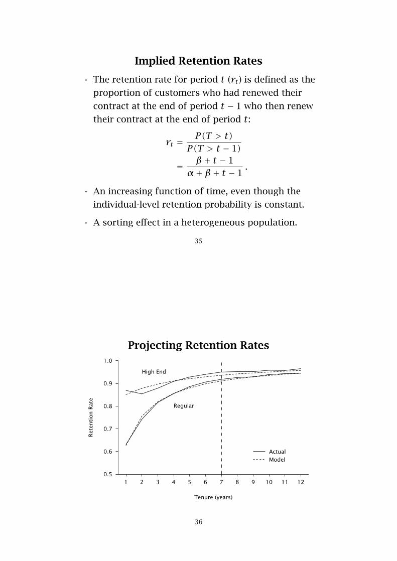
Implied Retention Rates
• The retention rate for period t (rt) is defined as the
proportion of customers who had renewed their
contract at the end of period t − 1 who then renew
their contract at the end of period t:
rt = P(T > t)P(T > t − 1)
= β+ t − 1α+ β+ t − 1
.
• An increasing function of time, even though the
individual-level retention probability is constant.
• A sorting effect in a heterogeneous population.
35
Projecting Retention Rates
1 2 3 4 5 6 7 8 9 10 11 12
Tenure (years)
0.5
0.6
0.7
0.8
0.9
1.0
Ret
enti
on
Rat
e
.................................................................................................
.........................................
..................................................
.................................................................................
.........................................................................................................................................................................................................................................................................................
..............
........................................................................................................................................................................................
................................
......................................
.............................................
........................................................................
........................................................................................................................................................
...............................................................................................................
Actual
............................
................................
......................................................
.......................................................................................
.......................................................................................................................................
..........................................................................................
..........................
......................
..............................
..........................................
...............................................................
............................................................................................................
Model
High End
Regular
36

Concepts and Tools Introduced
• Probability models
• Maximum-likelihood estimation of model
parameters
• Modeling discrete-time (single-event) duration data
• Models of contract renewal behavior
37
Further Reading
Buchanan, Bruce and Donald G. Morrison (1988), “A Stochastic
Model of List Falloff with Implications for Repeat Mailings,”
Journal of Direct Marketing, 2 (Summer), 7–15.
Fader, Peter S. and Bruce G. S. Hardie (2005), “A Simple
Probability Model for Projecting Customer Retention.”
[http://brucehardie.com/papers/021/]
Weinberg, Clarice Ring and Beth C. Gladen (1986), “The
Beta-Geometric Distribution Applied to Comparative
Fecundability Studies,” Biometrics, 42 (September), 547–560.
38

Introduction to Probability Models
39
The Logic of Probability Models
• Many researchers attempt to describe/predictbehavior using observed variables.
• However, they still use random components inrecognition that not all factors are included in themodel.
• We treat behavior as if it were “random”(probabilistic, stochastic).
• We propose a model of individual-level behaviorwhich is “summed” across individuals (takingindividual differences into account) to obtain amodel of aggregate behavior.
40

Uses of Probability Models
• Understanding market-level behavior patterns
• Prediction
– To settings (e.g., time periods) beyond theobservation period
– Conditional on past behavior
• Profiling behavioral propensities of individuals
• Benchmarks/norms
41
Building a Probability Model
(i) Determine the marketing decision problem/information needed.
(ii) Identify the observable individual-level behaviorof interest.
• We denote this by x.
(iii) Select a probability distribution thatcharacterizes this individual-level behavior.
• This is denoted by f(x|θ).• We view the parameters of this distribution
as individual-level latent characteristics.
42

Building a Probability Model
(iv) Specify a distribution to characterize thedistribution of the latent characteristicvariable(s) across the population.
• We denote this by g(θ).• This is often called the mixing distribution.
(v) Derive the corresponding aggregate or observeddistribution for the behavior of interest:
f(x) =∫f(x|θ)g(θ)dθ
43
Building a Probability Model
(vi) Estimate the parameters (of the mixingdistribution) by fitting the aggregatedistribution to the observed data.
(vii) Use the model to solve the marketing decisionproblem/provide the required information.
44

Outline• Problem 1: Projecting Customer Retention Rates
(Modeling Discrete-Time Duration Data)
• Problem 2: Predicting New Product Trial(Modeling Continuous-Time Duration Data)
• Problem 3: Estimating Billboard Exposures(Modeling Count Data)
• Problem 4: Test/Roll Decisions in Segmentation- basedDirect Marketing(Modeling “Choice” Data)
• Problem 5: Characterizing the Purchasing of Hard-Candy(Introduction to Finite Mixture Models)
• Problem 6: Who is Visiting khakichinos.com?(Incorporating Covariates in Count Models)
45
Problem 2:Predicting New Product Trial
(Modeling Continuous-Time Duration Data)
46

Background
Ace Snackfoods, Inc. has developed a new shelf-stable juiceproduct called Kiwi Bubbles. Before deciding whether or not to“go national” with the new product, the marketing manager forKiwi Bubbles has decided to commission a year-long test marketusing IRI’s BehaviorScan service, with a view to getting a clearerpicture of the product’s potential.
The product has now been under test for 24 weeks. On handis a dataset documenting the number of households that havemade a trial purchase by the end of each week. (The total size ofthe panel is 1499 households.)
The marketing manager for Kiwi Bubbles would like a forecastof the product’s year-end performance in the test market. First,she wants a forecast of the percentage of households that willhave made a trial purchase by week 52.
47
Kiwi Bubbles Cumulative Trial
Week # Households Week # Households
1 8 13 68
2 14 14 72
3 16 15 75
4 32 16 81
5 40 17 90
6 47 18 94
7 50 19 96
8 52 20 96
9 57 21 96
10 60 22 97
11 65 23 97
12 67 24 101
48
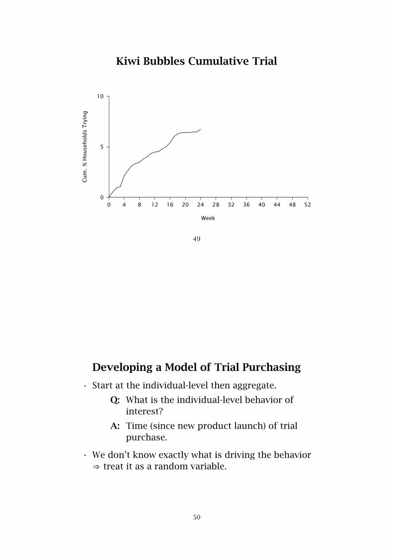
Kiwi Bubbles Cumulative Trial
0 4 8 12 16 20 24 28 32 36 40 44 48 52
Week
0
5
10
Cum
.%
House
hold
sT
ryin
g
................................................................................................................................................................
............................
...................................
....................................
..........................................................................................................
................................
49
Developing a Model of Trial Purchasing
• Start at the individual-level then aggregate.
Q: What is the individual-level behavior ofinterest?
A: Time (since new product launch) of trialpurchase.
• We don’t know exactly what is driving the behavior⇒ treat it as a random variable.
50
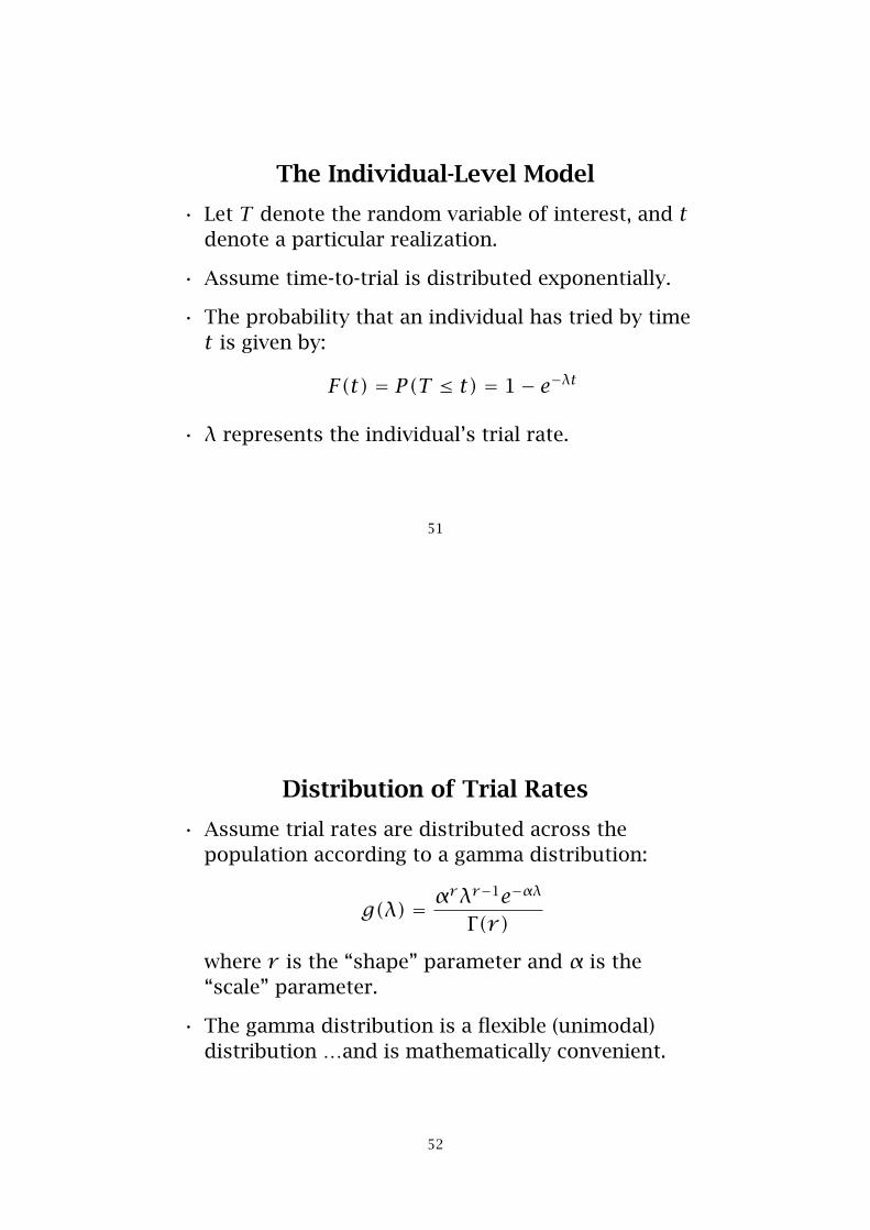
The Individual-Level Model
• Let T denote the random variable of interest, and tdenote a particular realization.
• Assume time-to-trial is distributed exponentially.
• The probability that an individual has tried by timet is given by:
F(t) = P(T ≤ t) = 1− e−λt
• λ represents the individual’s trial rate.
51
Distribution of Trial Rates
• Assume trial rates are distributed across thepopulation according to a gamma distribution:
g(λ) = αrλr−1e−αλ
Γ(r)
where r is the “shape” parameter and α is the“scale” parameter.
• The gamma distribution is a flexible (unimodal)distribution …and is mathematically convenient.
52
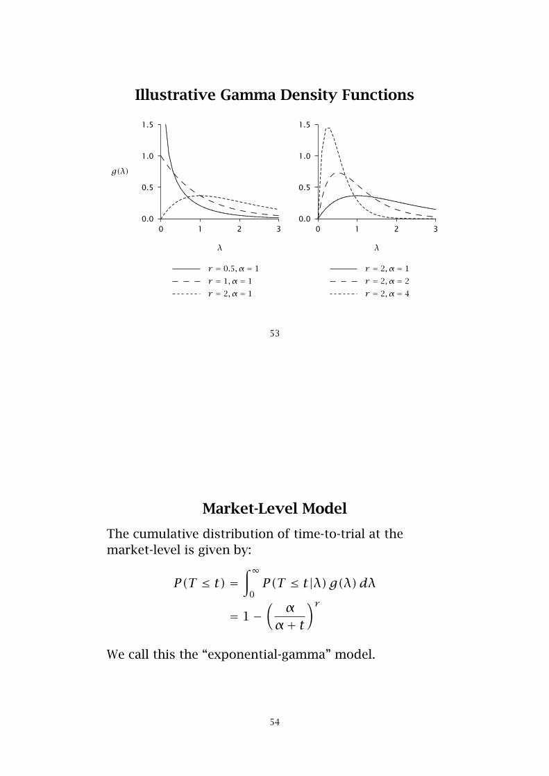
Illustrative Gamma Density Functions
0 1 2 3
λ
0.0
0.5
1.0
1.5
g(λ)
.................................................................................................................................................................................................................................................................................................................................................................................................................
r = 0.5, α = 1
..........................
..........................
............. ............. ............. ............. ............. ............. ............. ............. .............
r = 1, α = 1
....................................
..........................................................................................................................................
r = 2, α = 1
0 1 2 3
λ
0.0
0.5
1.0
1.5
..............................................................................
........................................................................................................................................................................................................................................
r = 2, α = 1
................................................................. ............. .............
.......................... ............. ............. ............. ............. ............. .............
r = 2, α = 2
......
......
......
......
......
......
......
......
......
......
......
......
......
......
......
....................................................................................................................................................................................................................................................................
r = 2, α = 4
53
Market-Level Model
The cumulative distribution of time-to-trial at themarket-level is given by:
P(T ≤ t) =∫∞
0P(T ≤ t|λ)g(λ)dλ
= 1−(
αα+ t
)rWe call this the “exponential-gamma” model.
54
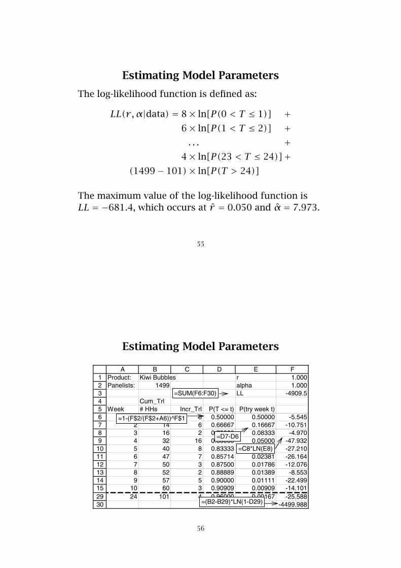
Estimating Model Parameters
The log-likelihood function is defined as:
LL(r ,α|data) = 8× ln[P(0 < T ≤ 1)] +6× ln[P(1 < T ≤ 2)] +. . . +
4× ln[P(23 < T ≤ 24)]+(1499− 101)× ln[P(T > 24)]
The maximum value of the log-likelihood function isLL = −681.4, which occurs at r̂ = 0.050 and α̂ = 7.973.
55
Estimating Model Parameters
1234567891011121314152930
A B C D E FProduct: Kiwi Bubbles r 1.000Panelists: 1499 alpha 1.000
LL -4909.5Cum_Trl
Week # HHs Incr_Trl P(T <= t) P(try week t)1 8 8 0.50000 0.50000 -5.5452 14 6 0.66667 0.16667 -10.7513 16 2 0.75000 0.08333 -4.9704 32 16 0.80000 0.05000 -47.9325 40 8 0.83333 0.03333 -27.2106 47 7 0.85714 0.02381 -26.1647 50 3 0.87500 0.01786 -12.0768 52 2 0.88889 0.01389 -8.5539 57 5 0.90000 0.01111 -22.499
10 60 3 0.90909 0.00909 -14.10124 101 4 0.96000 0.00167 -25.588
-4499.988
=1-(F$2/(F$2+A6))^F$1
=(B2-B29)*LN(1-D29)
=D7-D6
=SUM(F6:F30)
=C8*LN(E8)
56
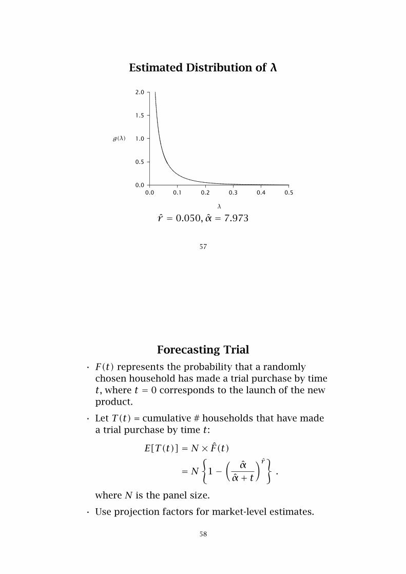
Estimated Distribution of λ
0.0 0.1 0.2 0.3 0.4 0.5
λ
0.0
0.5
1.0
1.5
2.0
g(λ)
................................................................................................................................................................................................................................................................................................................................................................................................................................................................................................................................................................................................................................................................................................................
r̂ = 0.050, α̂ = 7.973
57
Forecasting Trial
• F(t) represents the probability that a randomlychosen household has made a trial purchase by timet, where t = 0 corresponds to the launch of the newproduct.
• Let T(t) = cumulative # households that have madea trial purchase by time t:
E[T(t)] = N × F̂(t)
= N{
1−(
α̂α̂+ t
)r̂}.
where N is the panel size.
• Use projection factors for market-level estimates.
58
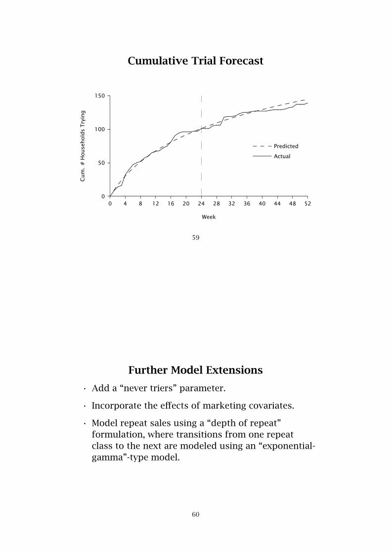
Cumulative Trial Forecast
0 4 8 12 16 20 24 28 32 36 40 44 48 52
Week
0
50
100
150
Cum
.#
House
hold
sT
ryin
g
...............................................................................................................................................................
............................
...................................
....................................
.............................................................................................................
...................................................................
..........................................................................................
.....................................................................
..........................................................................................................................................
..................................................
Actual
..............................................................................
..........................
..........................
..........................
..........................
..........................
.......................... ............. ............. ............. ............. ............. ............. ............. ............. ............. .............
Predicted
59
Further Model Extensions
• Add a “never triers” parameter.
• Incorporate the effects of marketing covariates.
• Model repeat sales using a “depth of repeat”formulation, where transitions from one repeatclass to the next are modeled using an “exponential-gamma”-type model.
60

Concepts and Tools Introduced
• Modeling continuous-time (single-event) durationdata
• Models of new product trial
61
Further ReadingFader, Peter S., Bruce G. S. Hardie, and Robert Zeithammer(2003), “Forecasting New Product Trial in a Controlled TestMarket Environment,” Journal of Forecasting, 22 (August),391–410.
Hardie, Bruce G. S., Peter S. Fader, and Michael Wisniewski(1998), “An Empirical Comparison of New Product TrialForecasting Models,” Journal of Forecasting, 17 (June–July),209–229.
Kalbfleisch, John D. and Ross L. Prentice (2002), The StatisticalAnalysis of Failure Time Data, 2nd edn., New York: Wiley.
Lawless, J. F. (1982), Statistical Models and Methods forLifetime Data, New York: Wiley.
62

Problem 3:Estimating Billboard Exposures
(Modeling Count Data)
63
Background
One advertising medium at the marketer’s disposal is theoutdoor billboard. The unit of purchase for this medium isusually a “monthly showing,” which comprises a specific set ofbillboards carrying the advertiser’s message in a given market.
The effectiveness of a monthly showing is evaluated in termsof three measures: reach, (average) frequency, and gross ratingpoints (GRPs). These measures are determined using datacollected from a sample of people in the market.
Respondents record their daily travel on maps. From eachrespondent’s travel map, the total frequency of exposure to theshowing over the survey period is counted. An “exposure” isdeemed to occur each time the respondent travels by a billboardin the showing, on the street or road closest to that billboard,going towards the billboard’s face.
64

Background
The standard approach to data collection requires eachrespondent to fill out daily travel maps for an entire month. Theproblem with this is that it is difficult and expensive to get a highproportion of respondents to do this accurately.
B&P Research is interested in developing a means by which itcan generate effectiveness measures for a monthly showing froma survey in which respondents fill out travel maps for only oneweek.
Data have been collected from a sample of 250 residents whocompleted daily travel maps for one week. The sampling processis such that approximately one quarter of the respondents fill outtravel maps during each of the four weeks in the target month.
65
Effectiveness Measures
The effectiveness of a monthly showing is evaluated interms of three measures:
• Reach: the proportion of the population exposed tothe billboard message at least once in the month.
• Average Frequency: the average number ofexposures (per month) among those people reached.
• Gross Rating Points (GRPs): the mean number ofexposures per 100 people.
66
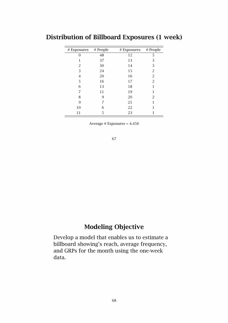
Distribution of Billboard Exposures (1 week)
# Exposures # People # Exposures # People
0 48 12 5
1 37 13 3
2 30 14 3
3 24 15 2
4 20 16 2
5 16 17 2
6 13 18 1
7 11 19 1
8 9 20 2
9 7 21 1
10 6 22 1
11 5 23 1
Average # Exposures = 4.456
67
Modeling Objective
Develop a model that enables us to estimate abillboard showing’s reach, average frequency,and GRPs for the month using the one-weekdata.
68

Modeling Issues
• Modeling the exposures to showing in a week.
• Estimating summary statistics of the exposuredistribution for a longer period of time (i.e., onemonth).
69
Model Development (I)
• Let the random variable X denote the number ofexposures to the showing in a week.
• At the individual-level, X is assumed to be Poissondistributed with (exposure) rate parameter λ:
P(X = x |λ) = λxe−λ
x!
• All individuals are assumed to have the sameexposure rate.
70
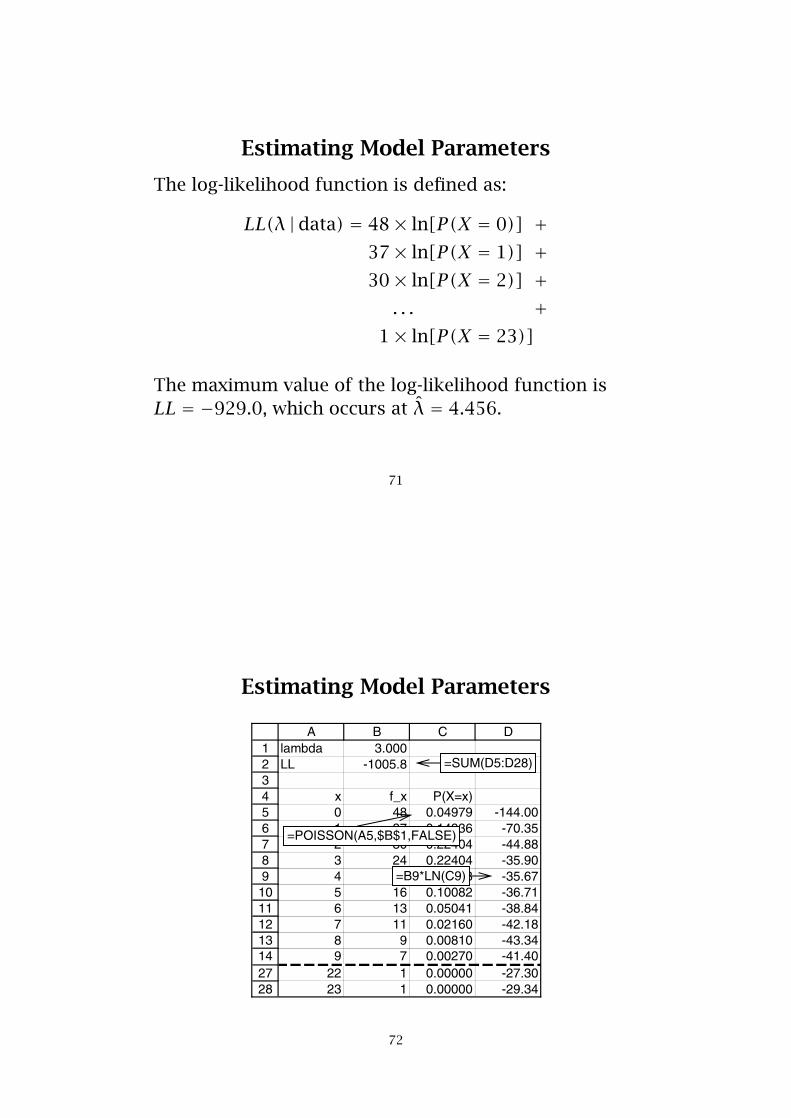
Estimating Model Parameters
The log-likelihood function is defined as:
LL(λ |data) = 48× ln[P(X = 0)] +37× ln[P(X = 1)] +30× ln[P(X = 2)] +. . . +
1× ln[P(X = 23)]
The maximum value of the log-likelihood function isLL = −929.0, which occurs at λ̂ = 4.456.
71
Estimating Model Parameters
123456789
10111213142728
A B C Dlambda 3.000LL -1005.8
x f_x P(X=x)0 48 0.04979 -144.001 37 0.14936 -70.352 30 0.22404 -44.883 24 0.22404 -35.904 20 0.16803 -35.675 16 0.10082 -36.716 13 0.05041 -38.847 11 0.02160 -42.188 9 0.00810 -43.349 7 0.00270 -41.40
22 1 0.00000 -27.3023 1 0.00000 -29.34
=POISSON(A5,$B$1,FALSE)
=SUM(D5:D28)
=B9*LN(C9)
72
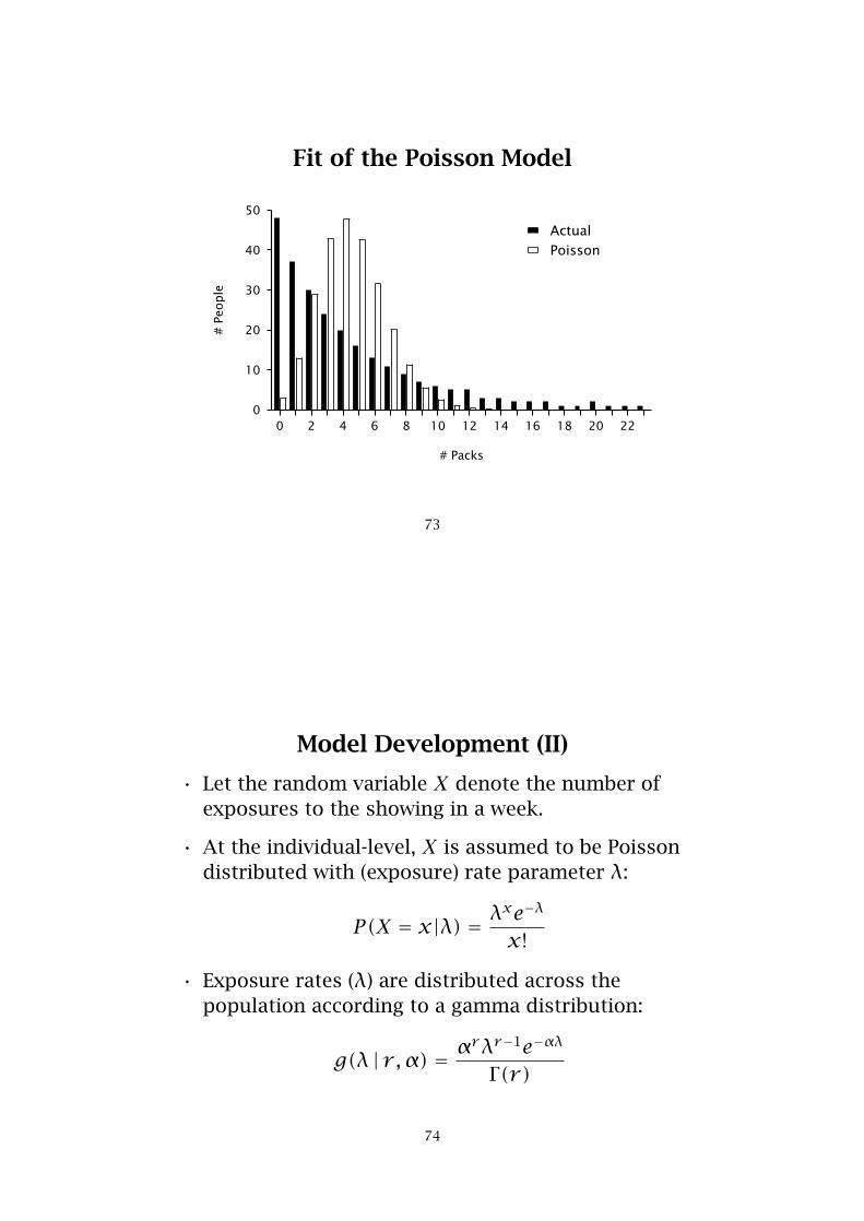
Fit of the Poisson Model
0 2 4 6 8 10 12 14 16 18 20 22
# Packs
0
10
20
30
40
50#
People
ActualPoisson
73
Model Development (II)
• Let the random variable X denote the number ofexposures to the showing in a week.
• At the individual-level, X is assumed to be Poissondistributed with (exposure) rate parameter λ:
P(X = x|λ) = λxe−λ
x!
• Exposure rates (λ) are distributed across thepopulation according to a gamma distribution:
g(λ | r ,α) = αrλr−1e−αλ
Γ(r)
74

Model Development (II)
The distribution of exposures at the population- level isgiven by:
P(X = x | r ,α) =∫∞
0P(X = x|λ)g(λ | r ,α)dλ
= Γ(r + x)Γ(r)x!
(α
α+ 1
)r ( 1α+ 1
)xThis is called the Negative Binomial Distribution, orNBD model.
75
Mean of the NBD
We can derive an expression for the mean of the NBD byconditioning:
E(X) = E[E(X |λ)]=∫∞
0E(X |λ)g(λ | r ,α)dλ
= rα.
76
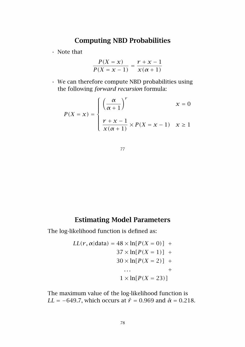
Computing NBD Probabilities
• Note that
P(X = x)P(X = x − 1)
= r + x − 1x(α+ 1)
• We can therefore compute NBD probabilities usingthe following forward recursion formula:
P(X = x) =
⎧⎪⎪⎪⎪⎪⎨⎪⎪⎪⎪⎪⎩
(α
α+ 1
)rx = 0
r + x − 1x(α+ 1)
× P(X = x − 1) x ≥ 1
77
Estimating Model Parameters
The log-likelihood function is defined as:
LL(r ,α|data) = 48× ln[P(X = 0)] +37× ln[P(X = 1)] +30× ln[P(X = 2)] +. . . +
1× ln[P(X = 23)]
The maximum value of the log-likelihood function isLL = −649.7, which occurs at r̂ = 0.969 and α̂ = 0.218.
78
Estimating Model Parameters
123456789
1011121314152829
A B C Dr 1.000alpha 1.000LL -945.5
x f_x P(X=x)0 48 0.50000 -33.271 37 0.25000 -51.292 30 0.12500 -62.383 24 0.06250 -66.544 20 0.03125 -69.315 16 0.01563 -66.546 13 0.00781 -63.087 11 0.00391 -61.008 9 0.00195 -56.149 7 0.00098 -48.52
22 1 0.00000 -15.9423 1 0.00000 -16.64
=(B2/(B2+1))^B1
=C6*($B$1+A7-1)/(A7*($B$2+1))
79
Estimated Distribution of λ
0.0
0.1
0.2
0.3
0.4
0.5
g(λ)
0 2 4 6 8 10
λ
.......................................................................................................................................................................................................................................................................................................................................................................................................................................................................................................................................................................................................................................................................
r̂ = 0.969, α̂ = 0.218
80

NBD for a Non-Unit Time Period
• Let X(t) be the number of exposures occuring in anobservation period of length t time units.
• If, for a unit time period, the distribution ofexposures at the individual-level is distributedPoisson with rate parameter λ, then X(t) has aPoisson distribution with rate parameter λt:
P(X(t) = x|λ) = (λt)xe−λt
x!
81
NBD for a Non-Unit Time Period
• The distribution of exposures at the population-level is given by:
P(X(t) = x | r ,α) =∫∞
0P(X(t) = x|λ)g(λ | r ,α)dλ
= Γ(r + x)Γ(r)x!
(α
α+ t)r ( t
α+ t)x
• The mean of this distribution is given by
E[X(t)] = rtα
82

Exposure Distributions: 1 week vs. 4 week
0 2 4 6 8 10 12 14 16 18 20+
# Exposures
0
30
60
90
#Pe
ople
1 week4 week
83
Effectiveness of Monthly Showing
• For t = 4, we have:
– P(X(t) = 0) = 0.056, and
– E[X(t)
] = 17.82
• It follows that:
– Reach = 1− P(X(t) = 0)= 94.4%
– Frequency = E[X(t)
]/(1− P(X(t) = 0)
)= 18.9
– GRPs = 100× E[X(t)]= 1782
84

Concepts and Tools Introduced
• Counting processes
• The NBD model
• Extrapolating an observed histogram over time
• Using models to estimate “exposure distributions”for media vehicles
85
Further ReadingEhrenberg, A. S. C. (1988), Repeat-Buying, 2nd edn., London:Charles Griffin & Company, Ltd. (Available online at<http://www.empgens.com/A/rb/rb.html>.)
Greene, Jerome D. (1982), Consumer Behavior Models forNon-Statisticians, New York: Praeger.
Morrison, Donald G. and David C. Schmittlein (1988),“Generalizing the NBD Model for Customer Purchases: WhatAre the Implications and Is It Worth the Effort?” Journal ofBusiness and Economic Statistics, 6 (April), 145–159.
86

Problem 4:Test/Roll Decisions in
Segmentation-based Direct Marketing
(Modeling “Choice” Data)
87
The “Segmentation” Approach
i. Divide the customer list into a set of (homogeneous)segments.
ii. Test customer response by mailing to a randomsample of each segment.
iii. Rollout to segments with a response rate (RR) abovesome cut-off point,
e.g., RR >cost of each mailing
unit margin
88

Ben’s Knick Knacks, Inc.
• A consumer durable product (unit margin =$161.50, mailing cost per 10,000 = $3343)
• 126 segments formed from customer database onthe basis of past purchase history information
• Test mailing to 3.24% of database
89
Ben’s Knick Knacks, Inc.
Standard approach:
• Rollout to all segments with
Test RR >3343/10,000
161.50= 0.00207
• 51 segments pass this hurdle
90
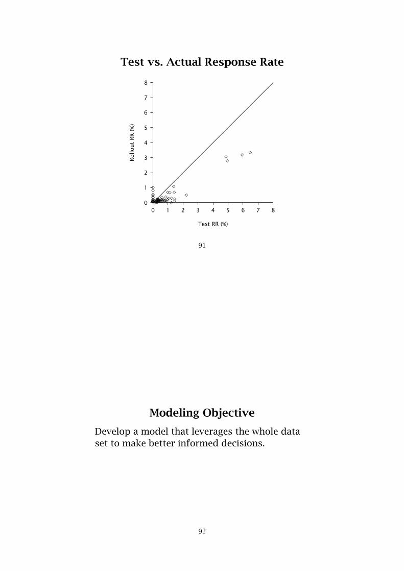
Test vs. Actual Response Rate
0 1 2 3 4 5 6 7 8
Test RR (%)
0
1
2
3
4
5
6
7
8
Rollo
ut
RR
(%)
� �� �
����
�������� ��� �� ��� ��������� ������� ����������� �� ������ �� ����� �����.................
...........................................................................................................................................................................................................................................................................................................................................................................................................................................................................................................................
91
Modeling Objective
Develop a model that leverages the whole dataset to make better informed decisions.
92
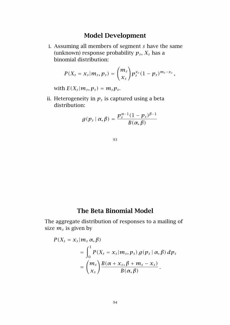
Model Development
i. Assuming all members of segment s have the same(unknown) response probability ps , Xs has abinomial distribution:
P(Xs = xs|ms,ps) =(ms
xs
)pxss (1− ps)ms−xs ,
with E(Xs|ms,ps) =msps .
ii. Heterogeneity in ps is captured using a betadistribution:
g(ps |α,β) = pα−1s (1− ps)β−1
B(α,β)
93
The Beta Binomial Model
The aggregate distribution of responses to a mailing ofsize ms is given by
P(Xs = xs|ms α,β)
=∫ 1
0P(Xs = xs|ms,ps)g(ps |α,β)dps
=(ms
xs
)B(α+ xs, β+ms − xs)
B(α,β).
94
Estimating Model Parameters
The log-likelihood function is defined as:
LL(α,β|data) =126∑s=1
ln[P(Xs = xs|ms,α,β)]
=126∑s=1
ln[
ms !(ms − xs)!xs !
Γ(α+ xs)Γ(β+ms − xs)Γ(α+ β+ms)︸ ︷︷ ︸B(α+xs,β+ms−xs)
Γ(α+ β)Γ(α)Γ(β)︸ ︷︷ ︸
1/B(α,β)
]
The maximum value of the log-likelihood function isLL = −200.5, which occurs at α̂ = 0.439 and β̂ = 95.411.
95
Estimating Model Parameters
123456789
1011121314
130131
A B C D Ealpha 1.000 B(alpha,beta) 1.000beta 1.000LL -718.9
Segment m_s x_s P(X=x|m)1 34 0 0.02857 -3.5552 102 1 0.00971 -4.6353 53 0 0.01852 -3.9894 145 2 0.00685 -4.9845 1254 62 0.00080 -7.1356 144 7 0.00690 -4.9777 1235 80 0.00081 -7.1208 573 34 0.00174 -6.3539 1083 24 0.00092 -6.988
125 383 0 0.00260 -5.951126 404 0 0.00247 -6.004
=SUM(E6:E131)
=COMBIN(B6,C6)*EXP(GAMMALN(B$1+C6)+GAMMALN(B$2+B6-C6)-GAMMALN(B$1+B$2+B6))/E$1
=LN(D11)
96
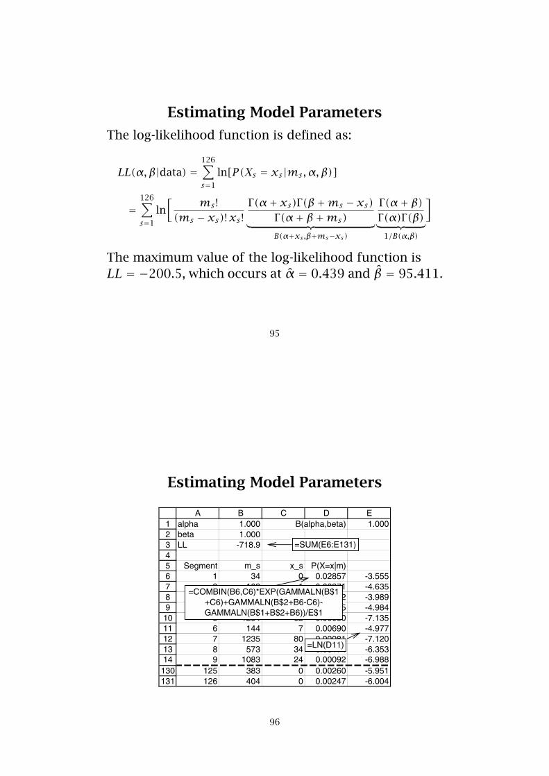
Estimated Distribution of p
0
5
10
15
20
g(p)
0.0 0.1 0.2 0.3 0.4 0.5 0.6 0.7 0.8 0.9 1.0
p
......................................................................................................................................................................................................................................................................................................................................................................................................................................................................................................................................................................................................................................................................................................................................................................................................................................................................................................
α̂ = 0.439, β̂ = 95.411, p̄ = 0.0046
97
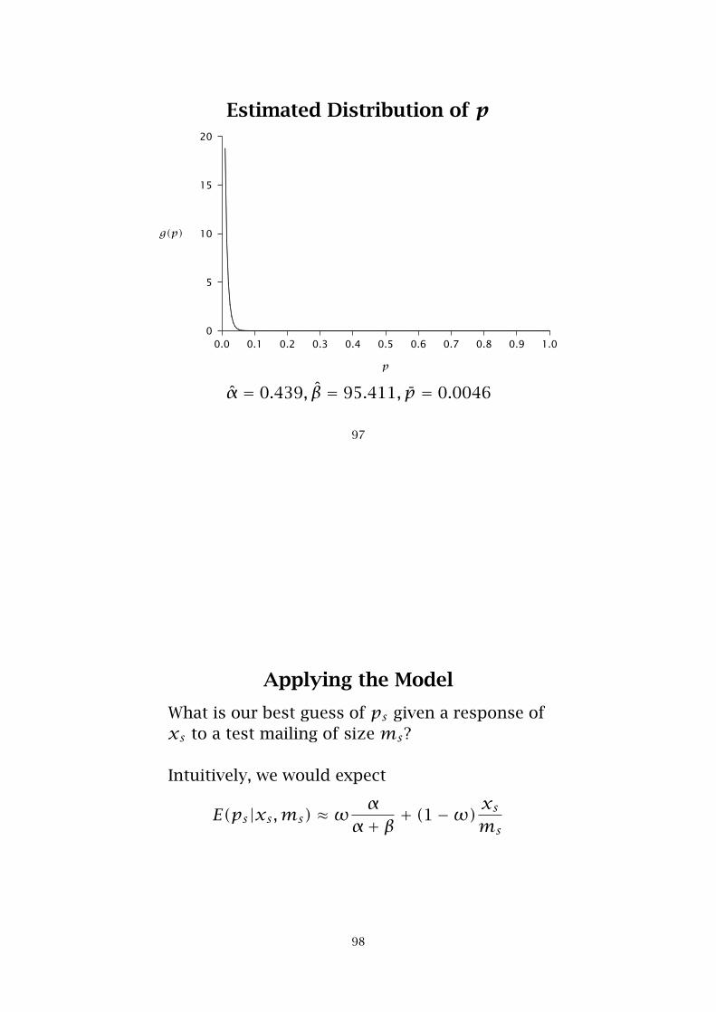
Applying the Model
What is our best guess of ps given a response ofxs to a test mailing of size ms?
Intuitively, we would expect
E(ps|xs,ms) ≈ω αα+ β + (1−ω)
xsms
98
Bayes Theorem
• The prior distribution g(p) captures the possiblevalues p can take on, prior to collecting anyinformation about the specific individual.
• The posterior distribution g(p|x) is the conditionaldistribution of p, given the observed data x. Itrepresents our updated opinion about the possiblevalues p can take on, now that we have someinformation x about the specific individual.
• According to Bayes theorem:
g(p|x) = f(x|p)g(p)∫f(x|p)g(p)dp
99
Bayes Theorem
For the beta-binomial model, we have:
g(ps|Xs = xs,ms) =
binomial︷ ︸︸ ︷P(Xs = xs|ms,ps)
beta︷ ︸︸ ︷g(ps)∫ 1
0P(Xs = xs|ms,ps)g(ps)dps︸ ︷︷ ︸
beta-binomial
= 1B(α+ xs, β+ms − xs)p
α+xs−1s (1− ps)β+ms−xs−1
which is a beta distribution with parameters α+ xs andβ+ms − xs .
100
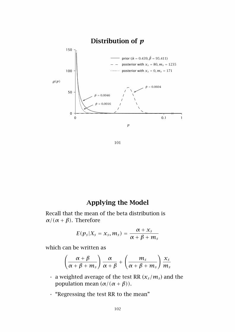
Distribution of p
0
50
100
150
g(p)
0 0.1 1
p
∼ ∼
..............................................................................................................................................................................................................................................................................................................................................................................................................................................................................................................................................................................................................................................................................................................................................................................................................................................................................
prior (α̂ = 0.439, β̂ = 95.411)
............. ............. ............. ............. ............. ............. ............. ............. ...........................................................................................
.................................................................
............. ............. ............. ............. .............
posterior with xs = 80,ms = 1235
....................................................................................................................................................................................................................................................................................................................................................................................................................................................................
posterior with xs = 0,ms = 171
.......................................................................
p̄ = 0.0604
.......................................................................
p̄ = 0.0016
.......................................................................
p̄ = 0.0046
101
Applying the Model
Recall that the mean of the beta distribution isα/(α+ β). Therefore
E(ps|Xs = xs,ms) = α+ xsα+ β+ms
which can be written as(α+ β
α+ β+ms
)α
α+ β +(
ms
α+ β+ms
)xsms
• a weighted average of the test RR (xs/ms) and thepopulation mean (α/(α+ β)).
• “Regressing the test RR to the mean”
102

Model-Based Decision Rule
• Rollout to segments with:
E(ps|Xs = xs,ms) >3343/10,000
161.5= 0.00207
• 66 segments pass this hurdle
• To test this model, we compare model predictionswith managers’ actions. (We also examine theperformance of the “standard” approach.)
103
Results
Standard Manager Model
# Segments (Rule) 51 66
# Segments (Act.) 46 71 53
Contacts 682,392 858,728 732,675
Responses 4,463 4,804 4,582
Profit $492,651 $488,773 $495,060
Use of model results in a profit increase of $6287;126,053 fewer contacts, saved for another offering.
104

Concepts and Tools Introduced
• “Choice” processes
• The Beta Binomial model
• “Regression-to-the-mean” and the use of models tocapture such an effect
• Bayes theorem (and “empirical Bayes” methods)
• Using “empirical Bayes” methods in thedevelopment of targeted marketing campaigns
105
Further ReadingColombo, Richard and Donald G. Morrison (1988),“Blacklisting Social Science Departments with Poor Ph.D.Submission Rates,” Management Science, 34 (June), 696–706.
Morrison, Donald G. and Manohar U. Kalwani (1993), “TheBest NFL Field Goal Kickers: Are They Lucky or Good?”Chance, 6 (August), 30–37.
Morwitz, Vicki G. and David C. Schmittlein (1998), “TestingNew Direct Marketing Offerings: The Interplay of ManagementJudgment and Statistical Models,” Management Science, 44(May), 610–628.
106

Problem 5:Characterizing the Purchasing of Hard-Candy
(Introduction to Finite Mixture Models)
107
Distribution of Hard-Candy Purchases
# Packs # People # Packs # People
0 102 11 10
1 54 12 10
2 49 13 3
3 62 14 3
4 44 15 5
5 25 16 5
6 26 17 4
7 15 18 1
8 15 19 2
9 10 20 1
10 10
Source: Dillon and Kumar (1994)
108
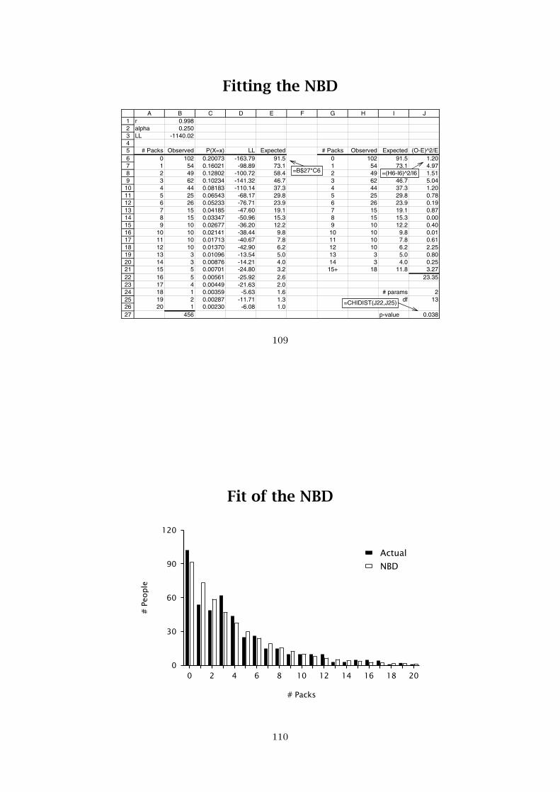
Fitting the NBD
123456789101112131415161718192021222324252627
A B C D E F G H I Jr 0.998alpha 0.250LL -1140.02
# Packs Observed P(X=x) LL Expected # Packs Observed Expected (O-E)^2/E0 102 0.20073 -163.79 91.5 0 102 91.5 1.201 54 0.16021 -98.89 73.1 1 54 73.1 4.972 49 0.12802 -100.72 58.4 2 49 58.4 1.513 62 0.10234 -141.32 46.7 3 62 46.7 5.044 44 0.08183 -110.14 37.3 4 44 37.3 1.205 25 0.06543 -68.17 29.8 5 25 29.8 0.786 26 0.05233 -76.71 23.9 6 26 23.9 0.197 15 0.04185 -47.60 19.1 7 15 19.1 0.878 15 0.03347 -50.96 15.3 8 15 15.3 0.009 10 0.02677 -36.20 12.2 9 10 12.2 0.40
10 10 0.02141 -38.44 9.8 10 10 9.8 0.0111 10 0.01713 -40.67 7.8 11 10 7.8 0.6112 10 0.01370 -42.90 6.2 12 10 6.2 2.2513 3 0.01096 -13.54 5.0 13 3 5.0 0.8014 3 0.00876 -14.21 4.0 14 3 4.0 0.2515 5 0.00701 -24.80 3.2 15+ 18 11.8 3.2716 5 0.00561 -25.92 2.6 23.3517 4 0.00449 -21.63 2.018 1 0.00359 -5.63 1.6 # params 219 2 0.00287 -11.71 1.3 df 1320 1 0.00230 -6.08 1.0
456 p-value 0.038
=B$27*C6 =(H6-I6)^2/I6
=CHIDIST(J22,J25)
109
Fit of the NBD
0 2 4 6 8 10 12 14 16 18 20
# Packs
0
30
60
90
120
#Pe
ople
Actual
NBD
110

The Zero-Inflated NBD Model
Because of the “excessive” number of zeros, let usconsider the zero-inflated NBD (ZNBD) model:
• a proportion π of the population never buyhard-candy
• the visiting behavior of the “ever buyers” can becharacterized by the NBD model
P(X = x) = δx=0π + (1−π)× Γ(r + x)
Γ(r)x!
(α
α+ 1
)r ( 1α+ 1
)xThis is sometimes called the “NBD with hard-corenon-buyers” model.
111
Fitting the ZNBD
1234567891011121314151617181920212223242526272829
A B C D E F G H I J Kr 1.504alpha 0.334pi 0.113LL -1136.17
P(X=x)# Packs Observed NBD ZNBD LL Expected # Packs Observed Expected (O-E)^2/E
0 102 0.12468 0.22368 -152.75 102.0 0 102 102.0 0.001 54 0.14054 0.12465 -112.44 56.8 1 54 56.8 0.142 49 0.13188 0.11697 -105.15 53.3 2 49 53.3 0.353 62 0.11545 0.10239 -141.29 46.7 3 62 46.7 5.024 44 0.09743 0.08641 -107.74 39.4 4 44 39.4 0.545 25 0.08039 0.07130 -66.02 32.5 5 25 32.5 1.746 26 0.06531 0.05793 -74.06 26.4 6 26 26.4 0.017 15 0.05248 0.04654 -46.01 21.2 7 15 21.2 1.828 15 0.04181 0.03708 -49.42 16.9 8 15 16.9 0.229 10 0.03309 0.02935 -35.28 13.4 9 10 13.4 0.86
10 10 0.02605 0.02311 -37.68 10.5 10 10 10.5 0.0311 10 0.02042 0.01811 -40.11 8.3 11 10 8.3 0.3712 10 0.01595 0.01415 -42.58 6.5 12 10 6.5 1.9513 3 0.01242 0.01101 -13.53 5.0 13 3 5.0 0.8114 3 0.00964 0.00855 -14.28 3.9 14 3 3.9 0.2115 5 0.00747 0.00663 -25.08 3.0 15+ 18 10.4 5.4816 5 0.00578 0.00512 -26.37 2.3 19.5417 4 0.00446 0.00395 -22.13 1.818 1 0.00343 0.00305 -5.79 1.4 # params 319 2 0.00264 0.00234 -12.11 1.1 df 1220 1 0.00203 0.00180 -6.32 0.8
456 p-value 0.076
=(A8=0)*B$3+(1-B$3)*C8
112

Fit of the ZNBD
0 2 4 6 8 10 12 14 16 18 20
# Packs
0
30
60
90
120#
People
Actual
ZNBD
113
What is Wrong With the NBD Model?
The assumptions underlying the model could be wrongon two accounts:
i. at the individual-level, the number of purchases isnot Poisson distributed
ii. purchase rates (λ) are not gamma-distributed
114
Relaxing the Gamma Assumption
• Replace the continuous distribution with a discretedistribution by allowing for multiple (discrete)segments each with a different (latent) buying rate:
P(X = x) =S∑s=1
πsP(X = x|λs),S∑s=1
πs = 1
• This is called a finite mixture model.
• We often reparameterize the mixing proportions forcomputational convenience:
πs = exp(θs)∑Ss′=1 exp(θs′)
, θS = 0.
115
Fitting the One-Segment Model
123456789
102526
A B C Dlambda 3.991LL -1545.00
# Packs Observed P(X=x) LL0 102 0.01848 -407.111 54 0.07375 -140.782 49 0.14717 -93.893 62 0.19579 -101.104 44 0.19536 -71.855 25 0.15595 -46.46
20 1 0.00000 -18.64456
116

Fitting the Two-Segment Model
123456789
1011122728
A B C D E Flambda_1 1.802lambda_2 9.121pi 0.701LL -1188.83
# Packs Observed Seg1 Seg2 P(X=x) LL0 102 0.16494 0.00011 0.11564 -220.041 54 0.29725 0.00100 0.20864 -84.632 49 0.26785 0.00455 0.18909 -81.613 62 0.16090 0.01383 0.11691 -133.074 44 0.07249 0.03154 0.06024 -123.615 25 0.02613 0.05753 0.03552 -83.44
20 1 0.00000 0.00071 0.00021 -8.45456
=POISSON(A7,B$1,FALSE)
=POISSON(A7,B$2,FALSE)=B$3*C7+(1-B$3)*D7
=B7*LN(E7)
117
Fitting the Two-Segment Model
118
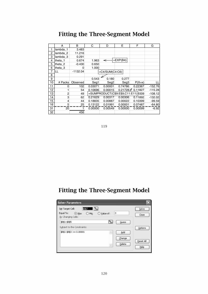
Fitting the Three-Segment Model
123456789
101112131415163132
A B C D E F Glambda_1 3.483lambda_2 11.216lambda_3 0.291theta_1 0.674 1.963theta_2 -0.430 0.650theta_3 0 1.000LL -1132.04
0.543 0.180 0.277# Packs Observed Seg1 Seg2 Seg3 P(X=x) LL
0 102 0.03071 0.00001 0.74786 0.22367 -152.761 54 0.10696 0.00015 0.21728 0.11827 -115.282 49 0.18628 0.00085 0.03157 0.11009 -108.123 62 0.21629 0.00317 0.00306 0.11892 -132.024 44 0.18835 0.00887 0.00022 0.10399 -99.595 25 0.13122 0.01991 0.00001 0.07487 -64.80
20 1 0.00000 0.00549 0.00000 0.00099 -6.92456
=EXP(B4)
=C4/SUM(C4:C6)
=SUMPRODUCT(C$9:E$9,C11:E11)
119
Fitting the Three-Segment Model
120
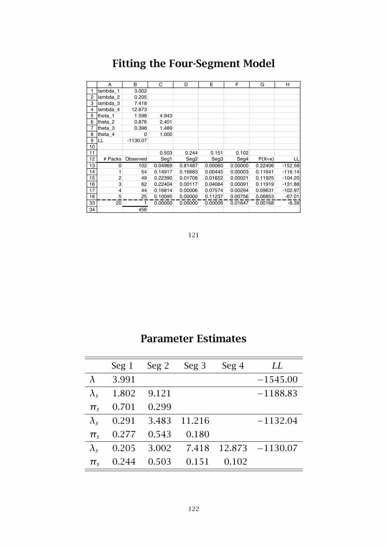
Fitting the Four-Segment Model
123456789
1011121314151617183334
A B C D E F G Hlambda_1 3.002lambda_2 0.205lambda_3 7.418lambda_4 12.873theta_1 1.598 4.943theta_2 0.876 2.401theta_3 0.398 1.489theta_4 0 1.000LL -1130.07
0.503 0.244 0.151 0.102# Packs Observed Seg1 Seg2 Seg3 Seg4 P(X=x) LL
0 102 0.04969 0.81487 0.00060 0.00000 0.22406 -152.581 54 0.14917 0.16683 0.00445 0.00003 0.11641 -116.142 49 0.22390 0.01708 0.01652 0.00021 0.11925 -104.203 62 0.22404 0.00117 0.04084 0.00091 0.11919 -131.884 44 0.16814 0.00006 0.07574 0.00294 0.09631 -102.975 25 0.10095 0.00000 0.11237 0.00756 0.06853 -67.01
20 1 0.00000 0.00000 0.00006 0.01647 0.00168 -6.39456
121
Parameter Estimates
Seg 1 Seg 2 Seg 3 Seg 4 LLλ 3.991 −1545.00
λs 1.802 9.121 −1188.83
πs 0.701 0.299
λs 0.291 3.483 11.216 −1132.04
πs 0.277 0.543 0.180
λs 0.205 3.002 7.418 12.873 −1130.07
πs 0.244 0.503 0.151 0.102
122

How Many Segments?
• Controlling for the extra parameters, is an S + 1segment model better than an S segment model?
• We can’t use the likelihood ratio test because itsproperties are violated
• It is standard practice to use “information-theoretic” model selection criteria
• A common measure is the Bayesian informationcriterion:
BIC = −2LL+ p ln(N)where p is the number of parameters and N is thesample size
• Rule: choose S to minimize BIC
123
Summary of Model Fit
Model LL # params BIC χ2 p-value
NBD −1140.02 2 2292.29 0.04
ZNBD −1136.17 3 2290.70 0.08
Poisson −1545.00 1 3096.12 0.00
2 seg Poisson −1188.83 3 2396.03 0.00
3 seg Poisson −1132.04 5 2294.70 0.22
4 seg Poisson −1130.07 7 2303.00 0.33
124
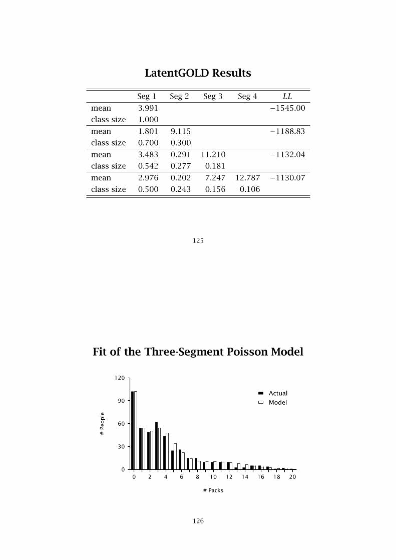
LatentGOLD Results
Seg 1 Seg 2 Seg 3 Seg 4 LLmean 3.991 −1545.00
class size 1.000
mean 1.801 9.115 −1188.83
class size 0.700 0.300
mean 3.483 0.291 11.210 −1132.04
class size 0.542 0.277 0.181
mean 2.976 0.202 7.247 12.787 −1130.07
class size 0.500 0.243 0.156 0.106
125
Fit of the Three-Segment Poisson Model
0 2 4 6 8 10 12 14 16 18 20
# Packs
0
30
60
90
120
#Pe
ople
Actual
Model
126
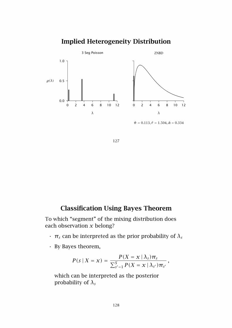
Implied Heterogeneity Distribution
3 Seg Poisson
0 2 4 6 8 10 12
λ
0.0
0.5
1.0
g(λ)
0 2 4 6 8 10 12
λ
........
........
........
........
........
........
........
........
........
.........
........
........
........
.........
........
.........
........
..........................................................................................................................................................................................................................................................................................................................................................................................................................................
ZNBD
π̂ = 0.113, r̂ = 1.504, α̂ = 0.334
127
Classification Using Bayes Theorem
To which “segment” of the mixing distribution doeseach observation x belong?
• πs can be interpreted as the prior probability of λs
• By Bayes theorem,
P(s |X = x) = P(X = x |λs)πs∑Ss′=1 P(X = x |λs′)πs′
,
which can be interpreted as the posteriorprobability of λs
128
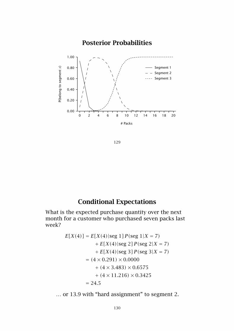
Posterior Probabilities
0 2 4 6 8 10 12 14 16 18 20
# Packs
0.00
0.20
0.40
0.60
0.80
1.00P(
bel
ong
tose
gm
ents)
...................................................................................................................................................................................................................................................................................................................................................................................................................................................................................................................................................................................................................................................................................................................................
Segment 1
...............................................................................................................................................
............. ............. ..........................
.....................................................................................................................
.......................... ............. ............. ............. ............. ............. ............. ............. ............. .............
Segment 2
..............................................................................
.............................................................................................................................................................................................
.......................................................................................................................................
Segment 3
129
Conditional Expectations
What is the expected purchase quantity over the nextmonth for a customer who purchased seven packs lastweek?
E[X(4)] = E[X(4)|seg 1] P(seg 1|X = 7)+ E[X(4)|seg 2] P(seg 2|X = 7)+ E[X(4)|seg 3] P(seg 3|X = 7)
= (4× 0.291)× 0.0000
+ (4× 3.483)× 0.6575
+ (4× 11.216)× 0.3425
= 24.5
… or 13.9 with “hard assignment” to segment 2.
130

Concepts and Tools Introduced
• Finite mixture models
• Discrete vs. continuous mixing distributions
• Probability models for classification
131
Further ReadingDillon, Wiliam R. and Ajith Kumar (1994), “Latent Structureand Other Mixture Models in Marketing: An Integrative Surveyand Overview,” in Richard P. Bagozzi (ed.), Advanced Methodsof Marketing Research, Oxford: Blackwell.
McLachlan, Geoffrey and David Peel (2000), Finite MixtureModels, New York: John Wiley & Sons.
Wedel, Michel and Wagner A. Kamakura (2000), MarketSegmentation: Conceptual and Methodological Foundations,2nd edn., Boston, MA: Kluwer Academic Publishers.
132

Problem 6:Who is Visiting khakichinos.com?
(Incorporating Covariates in Count Models)
133
BackgroundKhaki Chinos, Inc. is an established clothing catalog company
with an online presence at khakichinos.com. While the companyis able to track the online purchasing behavior of its customers, ithas no real idea as to the pattern of visiting behaviors by thebroader Internet population.
In order to gain an understanding of the aggregate visitingpatterns, some Media Metrix panel data has been purchased. Fora sample of 2728 people who visited an online apparel site atleast once during the second-half of 2000, the dataset reportshow many visits each person made to the khakichinos.com website, along with some demographic information.
Management would like to know whether frequency of visitingthe web site is related to demographic characteristics.
134
Raw Data
ID # Visits ln(Income) Sex ln(Age) HH Size
1 0 11.38 1 3.87 2
2 5 9.77 1 4.04 1
3 0 11.08 0 3.33 2
4 0 10.92 1 3.95 3
5 0 10.92 1 2.83 3
6 0 10.92 0 2.94 3
7 0 11.19 0 3.66 2
8 1 11.74 0 4.08 2
9 0 10.02 0 4.25 1
…
135
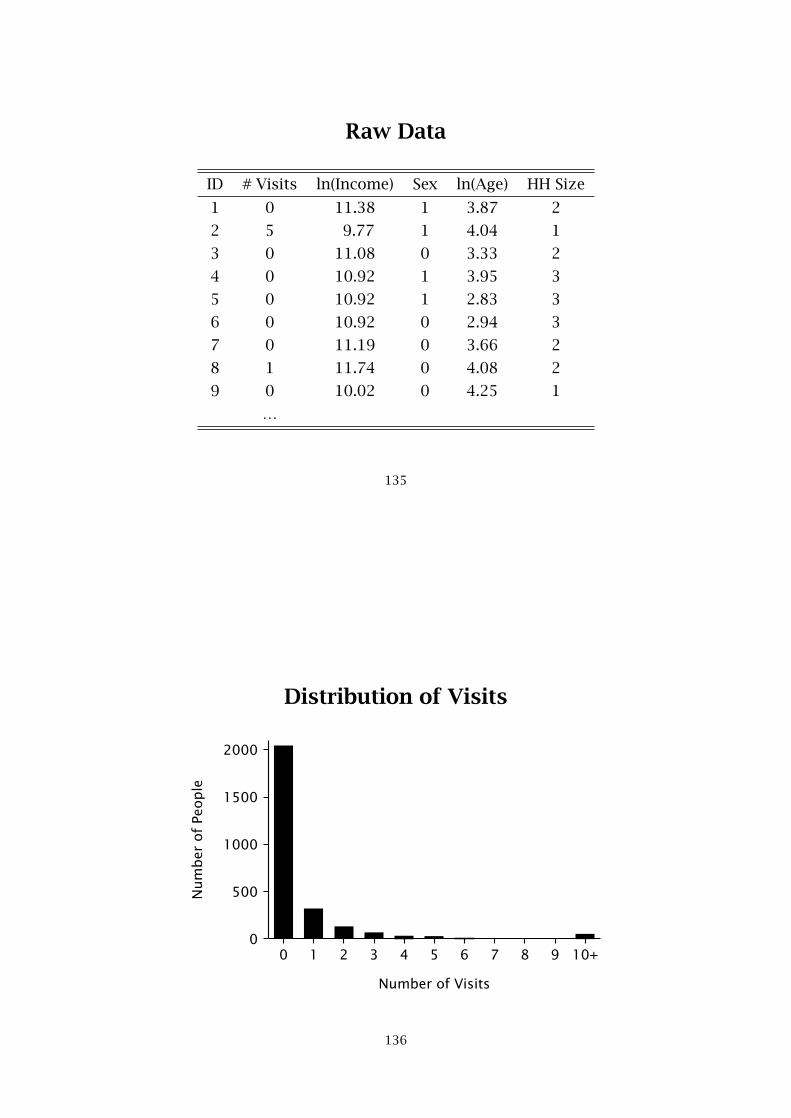
Distribution of Visits
0 1 2 3 4 5 6 7 8 9 10+
Number of Visits
0
500
1000
1500
2000
Num
ber
of
People
136

Modeling Count Data
Recall the NBD:
• At the individual-level, Y ∼ Poisson(λ)
• λ is distributed across the population according to agamma distribution with parameters r and α
P(Y = y) = Γ(r +y)Γ(r)y !
(α
α+ 1
)r ( 1α+ 1
)y
137
Observed vs. Unobserved Heterogeneity
Unobserved Heterogeneity:
• People differ in their mean (visiting) rate λ
• To account for heterogeneity in λ, we assume it isdistributed across the population according to some(parametric) distribution
• But there is no attempt to explain how people differ intheir mean rates
Observed Heterogeneity:
• We observe how people differ on a set of observableindependent (explanatory) variables
• We explicitly link an individual’s λ to her observablecharacteristics
138
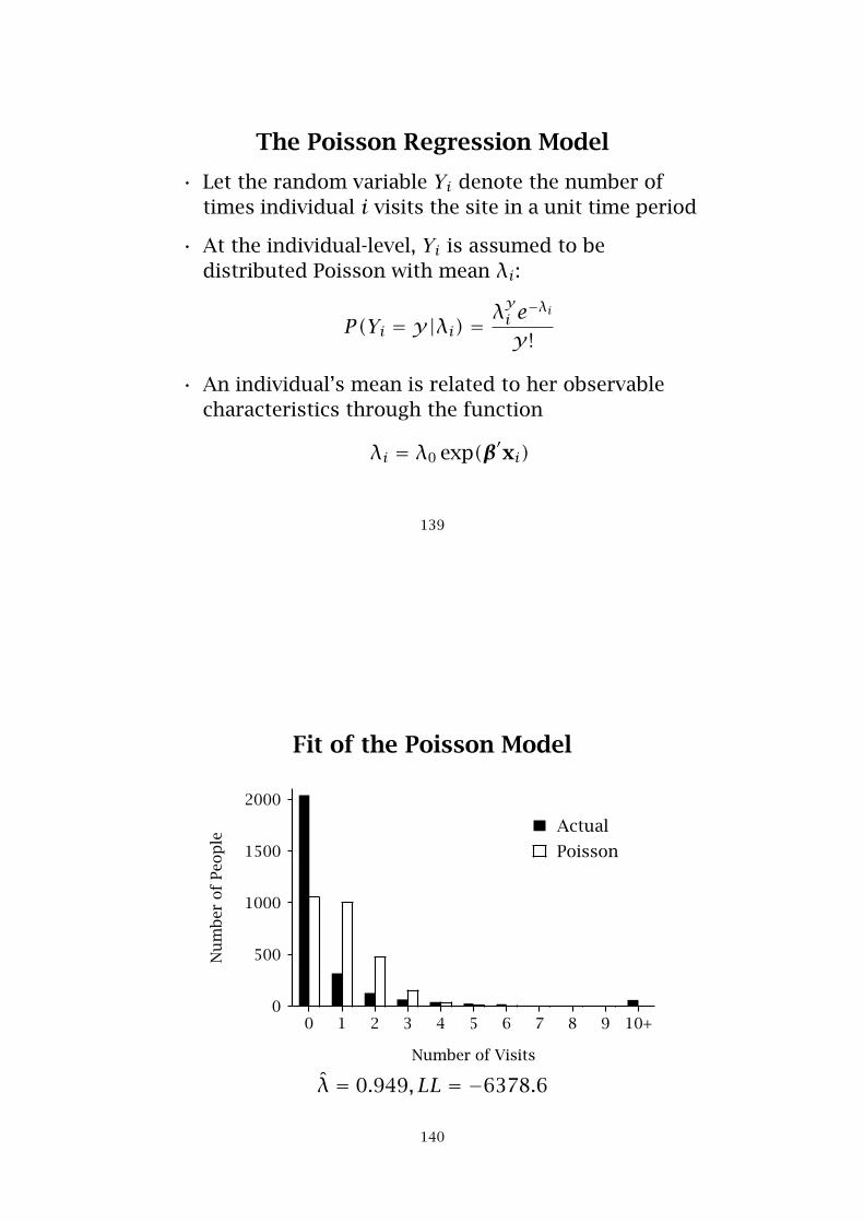
The Poisson Regression Model
• Let the random variable Yi denote the number oftimes individual i visits the site in a unit time period
• At the individual-level, Yi is assumed to bedistributed Poisson with mean λi:
P(Yi = y|λi) = λyi e−λi
y !
• An individual’s mean is related to her observablecharacteristics through the function
λi = λ0 exp(β′xi)
139
Fit of the Poisson Model
0 1 2 3 4 5 6 7 8 9 10+
Number of Visits
0
500
1000
1500
2000
Nu
mb
erof
Peo
ple
Actual
Poisson
λ̂ = 0.949, LL = −6378.6
140
Fitting the Poisson Regression Model
123456789101112131415161718
27352736
A B C D E F G H I J\lambda_0 0.0439 LL -6291.497B_inc 0.0938B_sex 0.0043B_age 0.5882B_size -0.0359
0.0938 0.0043 0.5882 -0.0359
ID Total Income Sex Age HH Size lambda P(Y=y) ln[P(Y=y)]1 0 11.38 1 3.87 2 1.16317 0.31249 -1.1632 5 9.77 1 4.04 1 1.14695 0.00525 -5.2493 0 11.08 0 3.33 2 0.82031 0.44030 -0.8204 0 10.92 1 3.95 3 1.12609 0.32430 -1.1265 0 10.92 1 2.83 3 0.58338 0.55801 -0.5836 0 10.92 0 2.94 3 0.62017 0.53785 -0.6207 0 11.19 0 3.66 2 1.00712 0.36527 -1.0078 1 11.74 0 4.08 2 1.35220 0.34977 -1.0509 0 10.02 0 4.25 1 1.31954 0.26726 -1.320
10 0 10.92 0 3.85 3 1.05656 0.34765 -1.0572727 0 10.53 1 2.89 4 0.56150 0.57035 -0.5612728 0 11.74 1 2.83 3 0.63010 0.53254 -0.630
=B$1*EXP(SUMPRODUCT(D$6:G$6,D9:G9))
=H9^B9*EXP(-H9)/FACT(B9)=LN(I9)
{=TRANSPOSE(B2:B5)}
141
Poisson Regression Results
Variable Coefficient
λ0 0.0439
Income 0.0938
Sex 0.0043
Age 0.5882
HH Size −0.0359
LL −6291.5LLPoiss −6378.6LR (df = 4) 174.2
142
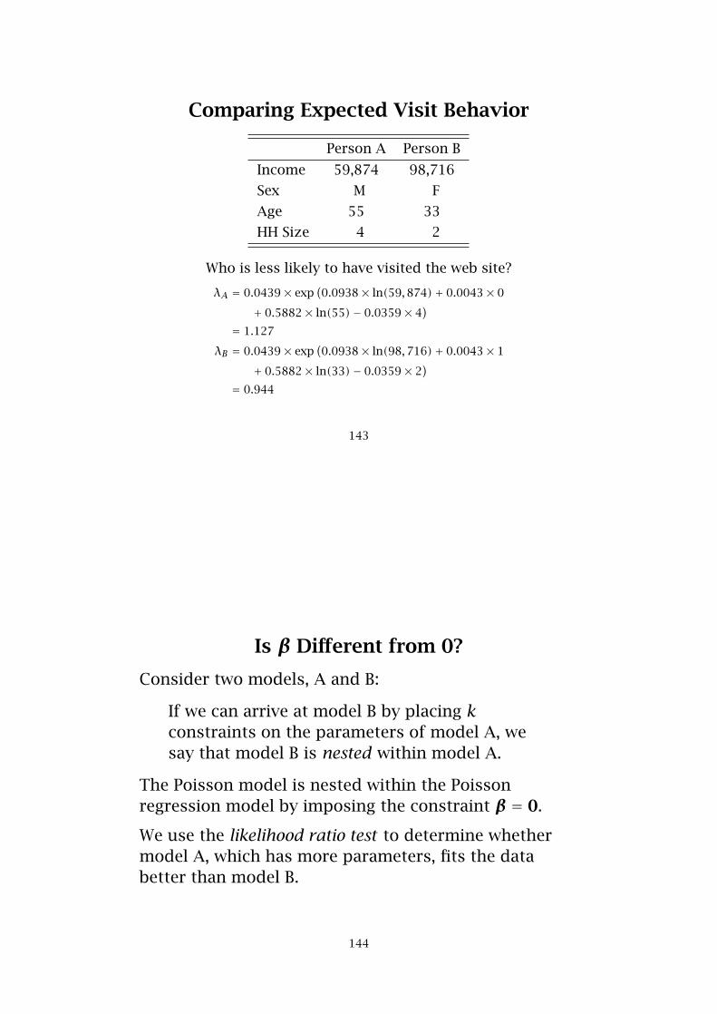
Comparing Expected Visit Behavior
Person A Person B
Income 59,874 98,716
Sex M F
Age 55 33
HH Size 4 2
Who is less likely to have visited the web site?
λA = 0.0439× exp(0.0938× ln(59,874)+ 0.0043× 0
+ 0.5882× ln(55)− 0.0359× 4)
= 1.127
λB = 0.0439× exp(0.0938× ln(98,716)+ 0.0043× 1
+ 0.5882× ln(33)− 0.0359× 2)
= 0.944
143
Is β Different from 0?
Consider two models, A and B:
If we can arrive at model B by placing kconstraints on the parameters of model A, wesay that model B is nested within model A.
The Poisson model is nested within the Poissonregression model by imposing the constraint β = 0.
We use the likelihood ratio test to determine whethermodel A, which has more parameters, fits the databetter than model B.
144

The Likelihood Ratio Test
• The null hypothesis is that model A is not differentfrom model B
• Compute the test statistic
LR = −2(LLB − LLA)
• Reject null hypothesis if LR > χ2.05,k
145
Computing Standard Errors
• Excel
– indirectly via a series of likelihood ratio tests
– easily computed from the Hessian matrix(computed using difference approximations)
• General modeling environments (e.g., MATLAB,Gauss)
– easily computed from the Hessian matrix (as aby-product of optimization or computed usingdifference approximations)
• Advanced statistics packages (e.g., Limdep, R, S-Plus)
– they come for free
146
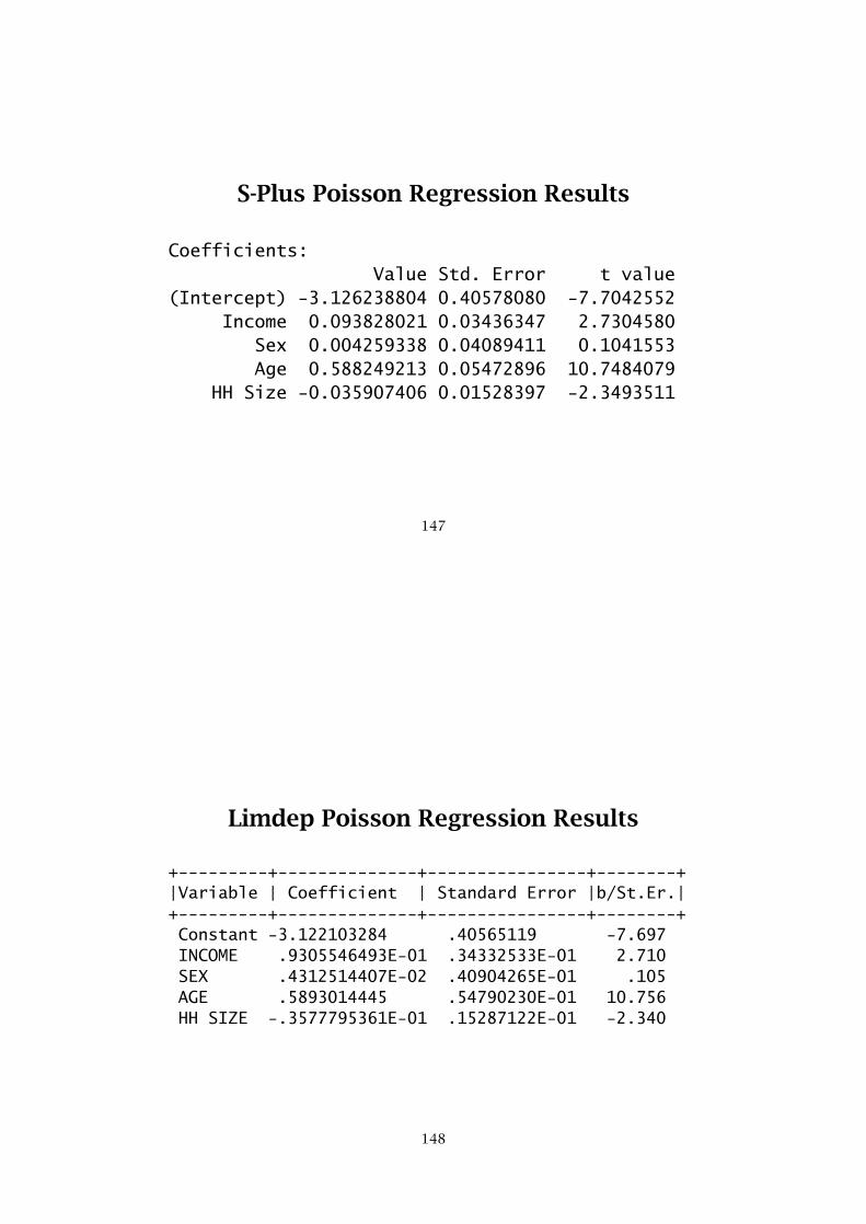
S-Plus Poisson Regression Results
Coefficients:Value Std. Error t value
(Intercept) -3.126238804 0.40578080 -7.7042552Income 0.093828021 0.03436347 2.7304580
Sex 0.004259338 0.04089411 0.1041553Age 0.588249213 0.05472896 10.7484079
HH Size -0.035907406 0.01528397 -2.3493511
147
Limdep Poisson Regression Results
+---------+--------------+----------------+--------+|Variable | Coefficient | Standard Error |b/St.Er.|+---------+--------------+----------------+--------+Constant -3.122103284 .40565119 -7.697INCOME .9305546493E-01 .34332533E-01 2.710SEX .4312514407E-02 .40904265E-01 .105AGE .5893014445 .54790230E-01 10.756HH SIZE -.3577795361E-01 .15287122E-01 -2.340
148
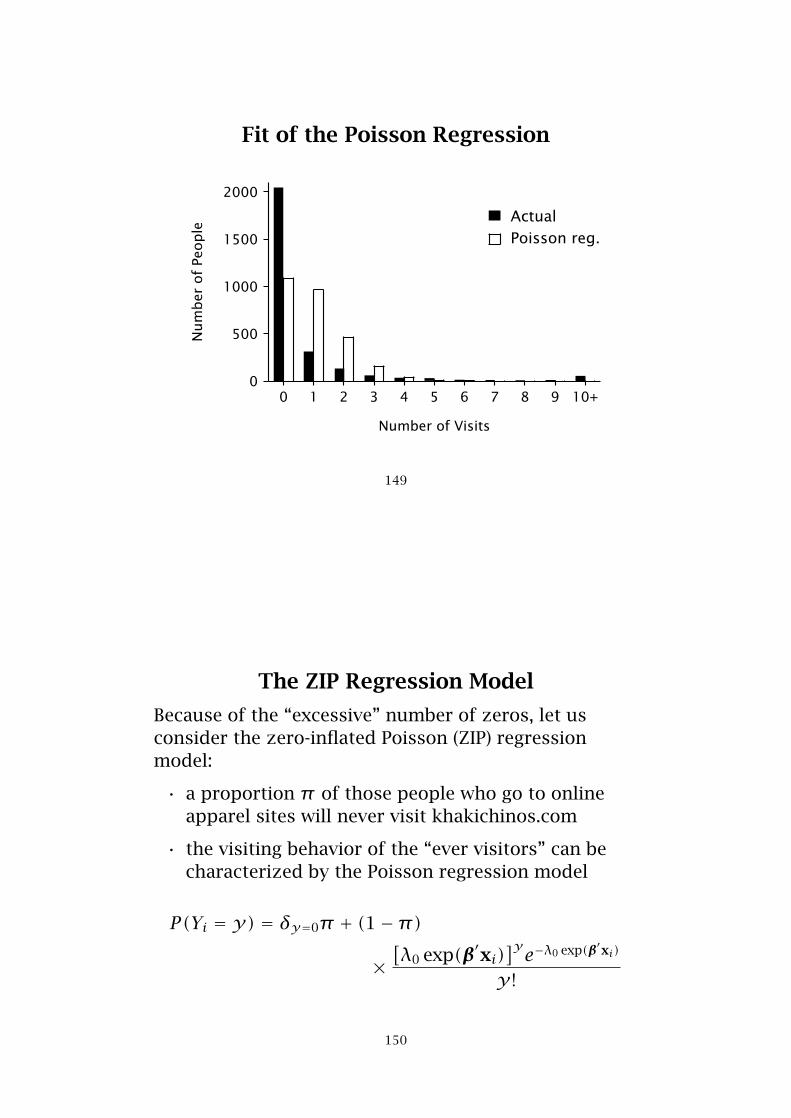
Fit of the Poisson Regression
0 1 2 3 4 5 6 7 8 9 10+
Number of Visits
0
500
1000
1500
2000N
um
ber
of
People
ActualPoisson reg.
149
The ZIP Regression Model
Because of the “excessive” number of zeros, let usconsider the zero-inflated Poisson (ZIP) regressionmodel:
• a proportion π of those people who go to onlineapparel sites will never visit khakichinos.com
• the visiting behavior of the “ever visitors” can becharacterized by the Poisson regression model
P(Yi = y) = δy=0π + (1−π)
×[λ0 exp(β′xi)
]ye−λ0 exp(β′xi)
y !
150
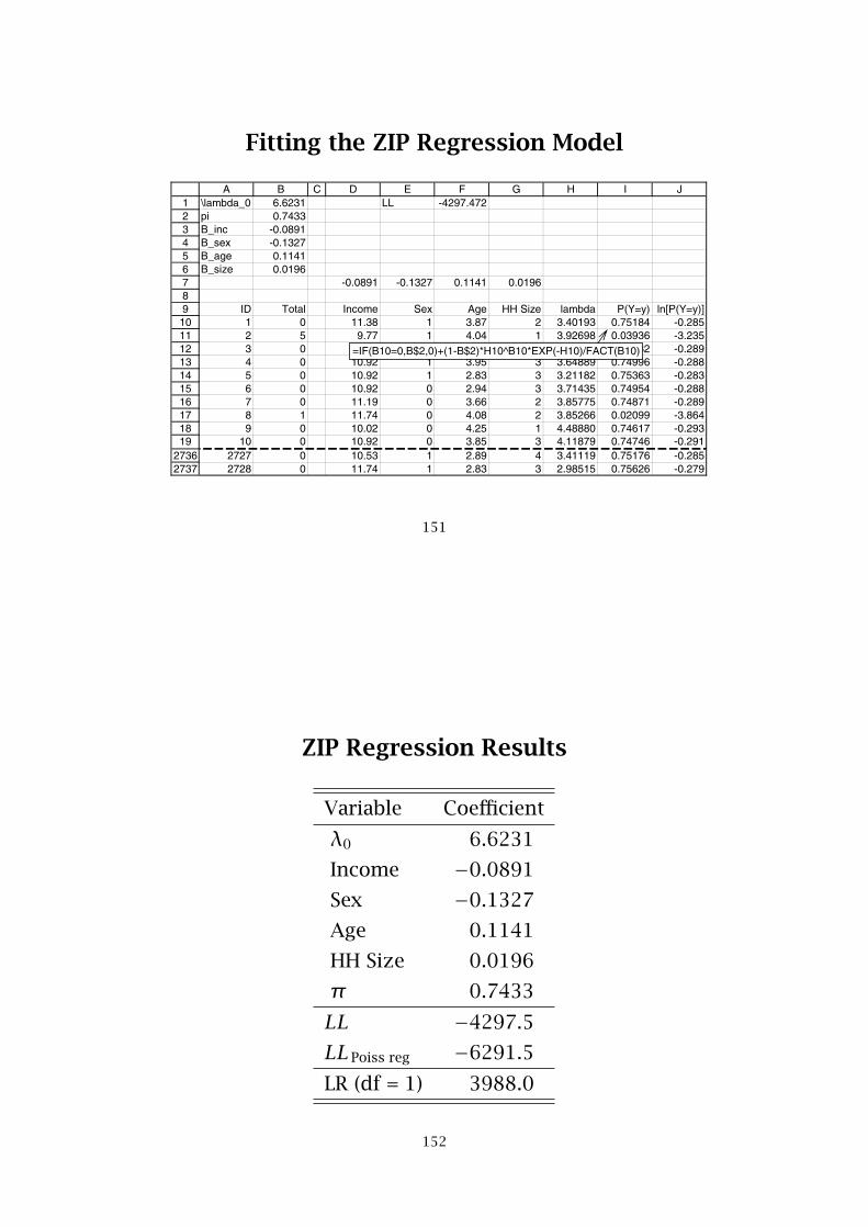
Fitting the ZIP Regression Model
123456789
10111213141516171819
27362737
A B C D E F G H I J\lambda_0 6.6231 LL -4297.472pi 0.7433B_inc -0.0891B_sex -0.1327B_age 0.1141B_size 0.0196
-0.0891 -0.1327 0.1141 0.0196
ID Total Income Sex Age HH Size lambda P(Y=y) ln[P(Y=y)]1 0 11.38 1 3.87 2 3.40193 0.75184 -0.2852 5 9.77 1 4.04 1 3.92698 0.03936 -3.2353 0 11.08 0 3.33 2 3.75094 0.74932 -0.2894 0 10.92 1 3.95 3 3.64889 0.74996 -0.2885 0 10.92 1 2.83 3 3.21182 0.75363 -0.2836 0 10.92 0 2.94 3 3.71435 0.74954 -0.2887 0 11.19 0 3.66 2 3.85775 0.74871 -0.2898 1 11.74 0 4.08 2 3.85266 0.02099 -3.8649 0 10.02 0 4.25 1 4.48880 0.74617 -0.293
10 0 10.92 0 3.85 3 4.11879 0.74746 -0.2912727 0 10.53 1 2.89 4 3.41119 0.75176 -0.2852728 0 11.74 1 2.83 3 2.98515 0.75626 -0.279
=IF(B10=0,B$2,0)+(1-B$2)*H10^B10*EXP(-H10)/FACT(B10)
151
ZIP Regression Results
Variable Coefficient
λ0 6.6231
Income −0.0891
Sex −0.1327
Age 0.1141
HH Size 0.0196
π 0.7433
LL −4297.5LLPoiss reg −6291.5LR (df = 1) 3988.0
152
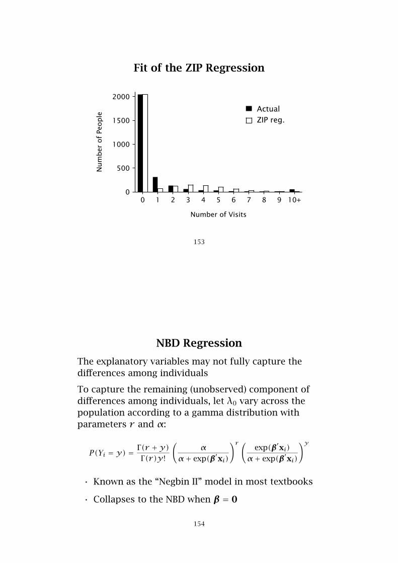
Fit of the ZIP Regression
0 1 2 3 4 5 6 7 8 9 10+
Number of Visits
0
500
1000
1500
2000N
um
ber
of
People
ActualZIP reg.
153
NBD Regression
The explanatory variables may not fully capture thedifferences among individuals
To capture the remaining (unobserved) component ofdifferences among individuals, let λ0 vary across thepopulation according to a gamma distribution withparameters r and α:
P(Yi = y) = Γ(r +y)Γ(r)y !
(α
α+ exp(β′xi)
)r (exp(β′xi)
α+ exp(β′xi)
)y
• Known as the “Negbin II” model in most textbooks
• Collapses to the NBD when β = 0
154
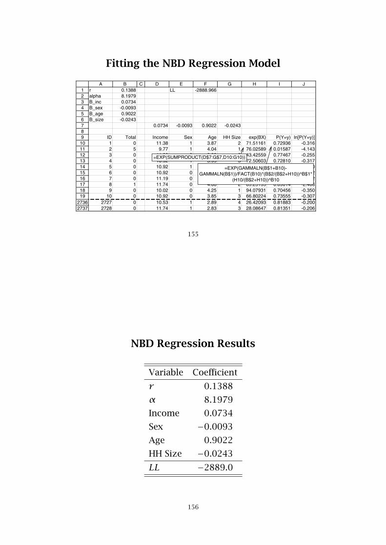
Fitting the NBD Regression Model
123456789
10111213141516171819
27362737
A B C D E F G H I Jr 0.1388 LL -2888.966alpha 8.1979B_inc 0.0734B_sex -0.0093B_age 0.9022B_size -0.0243
0.0734 -0.0093 0.9022 -0.0243
ID Total Income Sex Age HH Size exp(BX) P(Y=y) ln[P(Y=y)]1 0 11.38 1 3.87 2 71.51161 0.72936 -0.3162 5 9.77 1 4.04 1 76.02589 0.01587 -4.1433 0 11.08 0 3.33 2 43.42559 0.77467 -0.2554 0 10.92 1 3.95 3 72.50603 0.72810 -0.3175 0 10.92 1 2.83 3 26.44384 0.81876 -0.2006 0 10.92 0 2.94 3 29.50734 0.80919 -0.2127 0 11.19 0 3.66 2 59.02749 0.74680 -0.2928 1 11.74 0 4.08 2 89.25195 0.09014 -2.4069 0 10.02 0 4.25 1 94.07931 0.70456 -0.350
10 0 10.92 0 3.85 3 66.80224 0.73555 -0.3072727 0 10.53 1 2.89 4 26.42093 0.81883 -0.2002728 0 11.74 1 2.83 3 28.08647 0.81351 -0.206
=EXP(SUMPRODUCT(D$7:G$7,D10:G10))
=EXP(GAMMALN(B$1+B10)-GAMMALN(B$1))/FACT(B10)*(B$2/(B$2+H10))^B$1*
(H10/(B$2+H10))^B10
155
NBD Regression Results
Variable Coefficient
r 0.1388
α 8.1979
Income 0.0734
Sex −0.0093
Age 0.9022
HH Size −0.0243
LL −2889.0
156
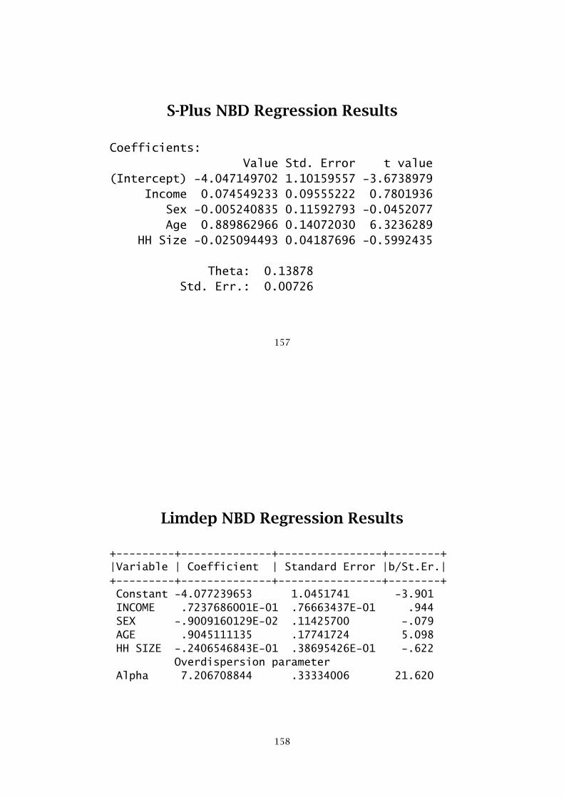
S-Plus NBD Regression Results
Coefficients:Value Std. Error t value
(Intercept) -4.047149702 1.10159557 -3.6738979Income 0.074549233 0.09555222 0.7801936
Sex -0.005240835 0.11592793 -0.0452077Age 0.889862966 0.14072030 6.3236289
HH Size -0.025094493 0.04187696 -0.5992435
Theta: 0.13878Std. Err.: 0.00726
157
Limdep NBD Regression Results
+---------+--------------+----------------+--------+|Variable | Coefficient | Standard Error |b/St.Er.|+---------+--------------+----------------+--------+Constant -4.077239653 1.0451741 -3.901INCOME .7237686001E-01 .76663437E-01 .944SEX -.9009160129E-02 .11425700 -.079AGE .9045111135 .17741724 5.098HH SIZE -.2406546843E-01 .38695426E-01 -.622
Overdispersion parameterAlpha 7.206708844 .33334006 21.620
158
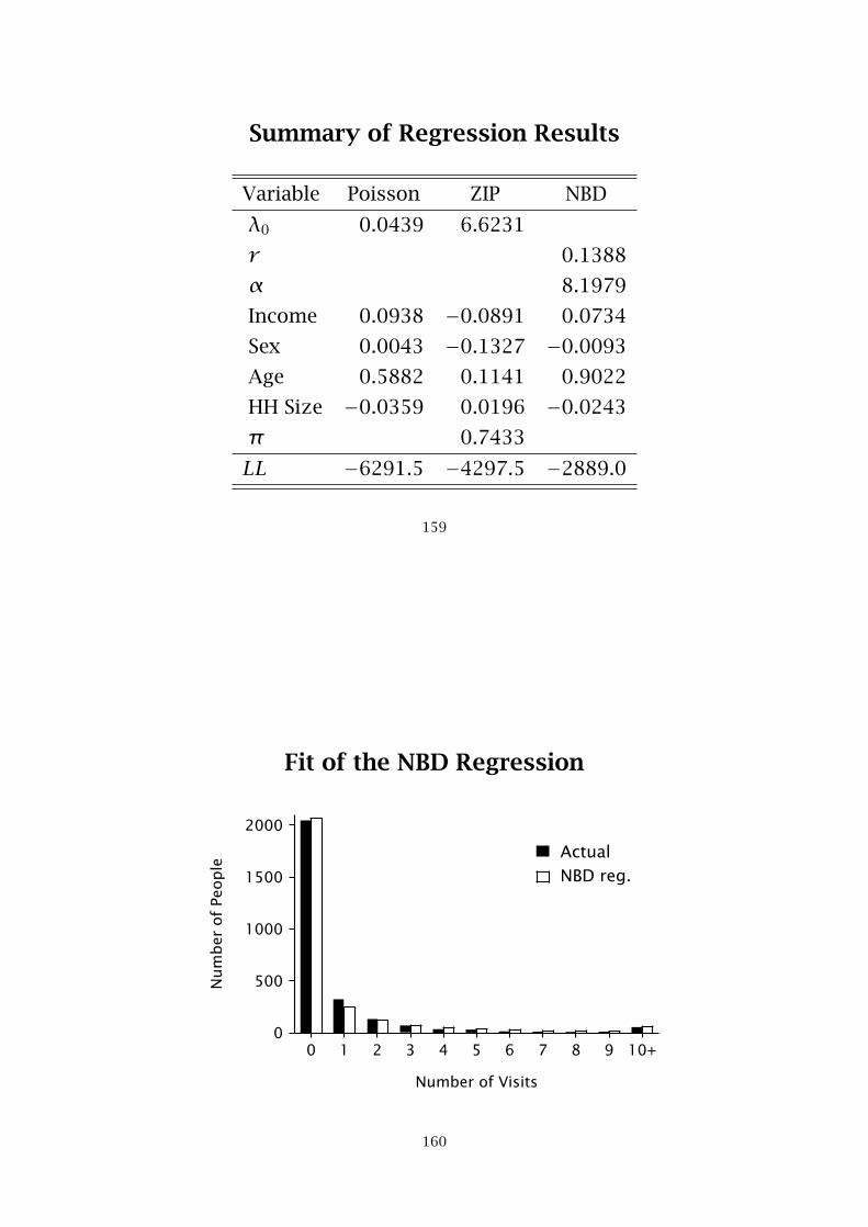
Summary of Regression Results
Variable Poisson ZIP NBD
λ0 0.0439 6.6231
r 0.1388
α 8.1979
Income 0.0938 −0.0891 0.0734
Sex 0.0043 −0.1327 −0.0093
Age 0.5882 0.1141 0.9022
HH Size −0.0359 0.0196 −0.0243
π 0.7433
LL −6291.5 −4297.5 −2889.0
159
Fit of the NBD Regression
0 1 2 3 4 5 6 7 8 9 10+
Number of Visits
0
500
1000
1500
2000
Num
ber
of
People
ActualNBD reg.
160
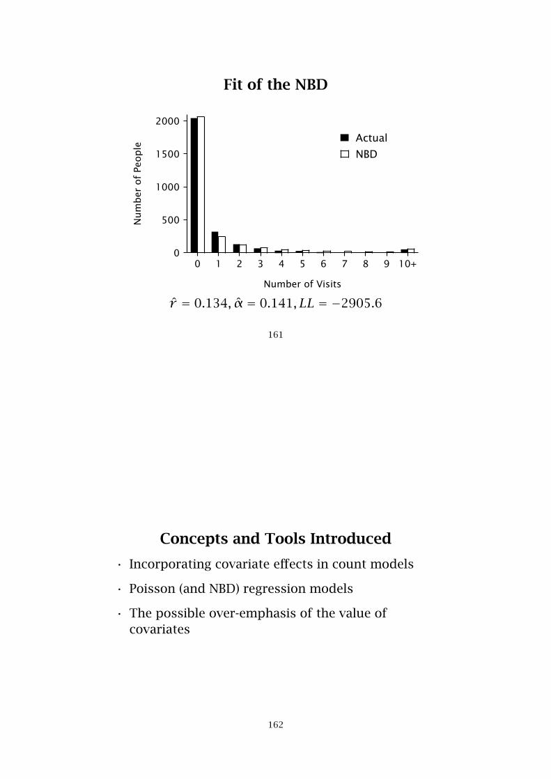
Fit of the NBD
0 1 2 3 4 5 6 7 8 9 10+
Number of Visits
0
500
1000
1500
2000
Num
ber
of
People
Actual
NBD
r̂ = 0.134, α̂ = 0.141, LL = −2905.6
161
Concepts and Tools Introduced
• Incorporating covariate effects in count models
• Poisson (and NBD) regression models
• The possible over-emphasis of the value ofcovariates
162
Further ReadingCameron, A. Colin and Pravin K. Trivedi (1998), RegressionAnalysis of Count Data, Cambridge: Cambridge UniversityPress.
Wedel, Michel and Wagner A. Kamakura (2000), MarketSegmentation: Conceptual and Methodological Foundations,2nd edn., Boston, MA: Kluwer Academic Publishers.
Winkelmann, Rainer (2003), Econometric Analysis of CountData, 4th edn., Berlin: Springer.
163
Introducing Covariates: The General Case
• Select a probability distribution that characterizes theindividual-level behavior of interest:
f(y|θi)• Make the individual-level latent characteristic(s) a
function of (time-invariant) covariates:
θi = s(θ0,xi)
• Specify a mixing distribution to capture theheterogeneity in θi not “explained” by xi
• Derive the corresponding aggregate distribution
f(y|xi) =∫f(y|θ0,xi)g(θ0)dθ0
164
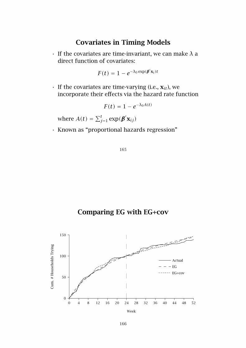
Covariates in Timing Models
• If the covariates are time-invariant, we can make λ adirect function of covariates:
F(t) = 1− e−λ0 exp(β′xi)t
• If the covariates are time-varying (i.e., xit), weincorporate their effects via the hazard rate function
F(t) = 1− e−λ0A(t)
where A(t) =∑tj=1 exp(β′xij)
• Known as “proportional hazards regression”
165
Comparing EG with EG+cov
0 4 8 12 16 20 24 28 32 36 40 44 48 52
Week
0
50
100
150
Cu
m.
#H
ou
seh
old
sT
ryin
g
...............................................................................................................................................................
............................
...................................
....................................
.............................................................................................................
...................................................................
..........................................................................................
.....................................................................
..........................................................................................................................................
..................................................
Actual
..............................................................................
..........................
..........................
..........................
..........................
..........................
.......................... ............. ............. ............. ............. ............. ............. ............. ............. ............. .............
EG
....................................................................................
........................................................
......................
........................
..................................
................................
........................................
......................................
....................................
..............................
..............................
............
EG+cov
166

Covariates in “Choice” Models
Two options for binary choice:
• The beta-logistic model
– a generalization of the beta-binomial model inwhich the mean is made a function of (time-invariant) covariates
– covariate effects not introduced at the level ofthe individual
• Finite mixture of binary logits:
P(Y = 1) = exp(β′xi)exp(β′xi)+ 1
with some elements of β varying across segments
167
Discussion
168
Recap
• The preceding six problems introduce simplemodels for three behavioral processes:
– Timing �→ “when”
– Counting �→ “how many”
– “Choice” �→ “whether/which”
• Each of these simple models has multipleapplications.
• More complex behavioral phenomena can becaptured by combining models from each of theseprocesses.
169
Further Applications: Timing Models
• Repeat purchasing of new products
• Response times:
– Coupon redemptions
– Survey response
– Direct mail (response, returns, repeat sales)
• Other durations:
– Salesforce job tenure
– Length of web site browsing session
170

Further Applications: Count Models
• Repeat purchasing
• Customer concentration (“80/20” rules)
• Salesforce productivity/allocation
• Number of page views during a web site browsingsession
171
Further Applications: “Choice” Models• Brand choice
HH #1 �×A
×B
×A
×A
HH #2 �×B
HH #3 �×B
×A
...
HH #h �×A
×B
×B
×B
• Media exposure
• Multibrand choice (BB → Dirichlet Multinomial)
• Taste tests (discrimination tests)
• “Click-through” behavior
172

Integrated Models
• Counting + Timing
– catalog purchases (purchasing | “alive” & “death” process)
– “stickiness” (# visits & duration/visit)
• Counting + Counting
– purchase volume (# transactions & units/transaction)
– page views/month (# visits & pages/visit)
• Counting + Choice
– brand purchasing (category purchasing & brand choice)
– “conversion” behavior (# visits & buy/not-buy)
173
A Template for Integrated Models
Stage 2
Counting Timing Choice
Counting
Stage 1 Timing
Choice
174

The Excel spreadsheets associated with this tutorial,along with electronic copies of the tutorial materials,can be found at:
http://brucehardie.com/talks.html
175